Galaxy properties from the outskirts to the core of a protocluster at $\mathbf{z=3.699}$

Abstract

We present follow-up spectroscopy on a protocluster candidate selected from the wide-field imaging of the Hyper SuprimeCam Subaru Strategic Programme. The target protocluster candidate was identified as a $4.5\sigma$ overdense region of $g$-dropout galaxies, and the redshifts of $g$-dropout galaxies are determined by detecting their Ly$\alpha$ emission. Thirteen galaxies, at least, are found to be clustering in the narrow redshift range of $\Delta z<0.05$ at $z=3.699$. This is clear evidence of the presence of a protocluster in the target region. Following the discovery of the protocluster at $z=3.699$, the physical properties and three-dimensional distribution of its member galaxies are investigated. Based on spectroscopically-confirmed $g$-dropout galaxies, we find an overabundance of rest-frame ultraviolet (UV) bright galaxies in the protocluster. The UV brightest protocluster member turns out to be an active galactic nucleus, and the other UV brighter members tend to show smaller Ly$\alpha$ equivalent widths than field counterparts. The member galaxies tend to densely populate near the centre of the protocluster, but the separation from the nearest neighbour rather than the distance from the centre of the protocluster is more tightly correlated to galaxy properties, implying that the protocluster is still in an early phase of cluster formation and only close neighbours have a significant impact on the physical properties of protocluster members. The number density of massive galaxies, selected from an archival photometric-redshift catalogue, is higher near the centre of the protocluster, while dusty starburst galaxies are distributed on the outskirts. These observational results suggest that the protocluster consists of multiple galaxy populations, whose spatial distributions may hint at the developmental phase of the galaxy cluster.

1 Introduction

Galaxy clusters are the most massive gravitationally-bound structures in the universe, formed from small perturbations in the density field when the universe was young. In the local universe, galaxy clusters occupy a unique position within the large-scale structure, namely at the nodes of the cosmic web (e.g., Peebles, 1980; Alpaslan et al., 2014; Libeskind et al., 2018); thus, the abundance or spatial distribution of galaxy clusters are powerful tools to constrain cosmological parameters (e.g., Hoessel et al., 1980; Fumagalli et al., 2024; Ghirardini et al., 2024). In addition, cluster galaxies possess distinguishing characteristics from field galaxies (e.g., Dressler, 1980; Wetzel et al., 2012; Gallazzi et al., 2021), suggesting that galaxy clusters have played a key role as the drivers of environmental effects on galaxy evolution. Consequently, galaxy clusters are a crucial bridge between galaxy evolution and the growth of cosmic structures, and equivalently between astrophysical and cosmological phenomena.

It remains challenging to predict how galaxies formed and evolved within a cosmological framework. The combination of $N$-body dark matter simulations and semi-analytic galaxy formation models enables such modelling over large cosmological volumes (e.g., Springel et al., 2005), though a significant number of parameters need to be tuned to reproduce observational results of galaxy properties (e.g., Ayromlou et al., 2019; Henriques et al., 2020). While hydrodynamical simulations can more directly trace the effects of physical processes (e.g., Barnes et al., 2017; Nelson et al., 2023), their larger computational expense introduces an unavoidable trade-off between mass resolution and size of the cosmological box being simulated. Therefore, it is also imperative to -alongside modelling endeavours- directly observe the developmental phase of galaxy clusters, so-called “protoclusters.”

Theoretical models predict that the size of protoclusters, or the spatial distribution of member galaxies, ranges from $\sim 1\,\mathrm{proper\,Mpc}$ (pMpc) up to $\sim 10\,\mathrm{pMpc}$ depending on their descendant halo mass at $z=0$ (Chiang et al., 2013; Muldrew et al., 2015). Furthermore, the shape of protoclusters is not spherical, but reflects the cosmic web (Lovell et al., 2018). Even at $z\lesssim 0.5$, about three quarters of galaxy clusters remain dynamically unrelaxed (e.g., Wen & Han, 2013; Yuan et al., 2022).

Observationally, protoclusters are identified by overdense regions of high-redshift galaxies, though many (slightly) different selection techniques are applied. The main challenge to protocluster searches is the rarity of protoclusters. To overcome this, some studies utilise quasars (QSOs) or radio galaxies (RGs) as signposts, because such massive galaxies are expected to reside in highly biased environments (e.g., Venemans et al., 2007; Wylezalek et al., 2013; Luo et al., 2022). Similarly, Ly$\alpha$ blobs (LABs) and bright sub-mm galaxies (SMGs) have also been successfully targeted to find protoclusters (e.g., Matsuda et al., 2011; Clements et al., 2016; Calvi et al., 2023). These signpost techniques would be efficient, but the relation between protoclusters and such peculiar galaxies (e.g., whether every protocluster hosts them) is still under debate (e.g., Hatch et al., 2014; Uchiyama et al., 2018; Gao et al., 2022). An alternative approach consists of mapping sufficiently wide areas on the sky, without requiring any extreme signposts as a prior, thus enabling the construction of a less biased sample of protoclusters (e.g., Ouchi et al., 2005; Toshikawa et al., 2012; Lemaux et al., 2018).

Making full use of various techniques, the number of known protoclusters are increasing (Overzier, 2016; Alberts & Noble, 2022). In contrast to mature clusters as seen in the local universe, protoclusters are composed of star-forming galaxies, and the relation between star-formation rate (SFR) and density is reversed (Lemaux et al., 2022; Shi et al., 2024). Protoclusters at high redshifts are expected to account for a significant fraction of cosmic SFR in spite of the rarity of these compact structures (e.g., Casey, 2016; Kato et al., 2016). Some extreme examples of protoclusters reach total star formation rates of $\gtrsim 10^{4}\,\mathrm{M_{\sun}\,yr^{-1}}$ in a single system (Miller et al., 2018; Oteo et al., 2018; Hill et al., 2020). Such intense star-forming activity may be sustained by a large amount of gas accreting along the cosmic web (Umehata et al., 2019; Daddi et al., 2022). An increased frequency of mergers/interactions may further boost the total SFR by triggering starburst phases. On the other hand, massive, quiescent galaxies also exist in protoclusters, at least as early as $z\sim 2\mathrm{-}4$ (Kubo et al., 2021; Ito et al., 2023; Tanaka et al., 2023). Toshikawa et al. (2016) confirmed several protoclusters from the same survey with a consistent method; however, they exhibit different features from each other. Toshikawa et al. (2020) discovered two protoclusters at $z\sim 3.7$: one shows a centrally concentrated distribution of protocluster members like a core, while the other is divided into several sub-groups. In addition, the fraction of massive quiescent galaxies among protocluster galaxies also differs from sample to sample even at the same redshift (Shi et al., 2020, 2021). As the history of cluster formation develops over Hubble timescales, protocluster structures and properties can vary significantly depending on their developmental phase. The descendant halo mass at $z=0$ is an important parameter in this context, but in practice can only be empirically constrained in a statistical manner (Press & Schechter, 1974). Even a precise measurement of the halo mass at the (high-redshift) epoch of observation will result in a $\sim 1\,\mathrm{dex}$ uncertainty on the descendant halo mass at $z=0$. This large range makes it difficult to fairly compare protoclusters, further compounded by observational biases.

The Subaru telescope carried out an unprecedented wide and deep imaging survey with Hyper Suprime-Cam (HSC; Miyazaki et al., 2018). The Subaru Strategic Programme with HSC (HSC-SSP; Aihara et al., 2018) is composed of three layers: Wide ($\sim 1,000\,\mathrm{deg^{2}}$, $i$-band depth of $m_{i}\sim 26.0\,\mathrm{mag}$), Deep ($\sim 25\,\mathrm{deg^{2}}$, $m_{i}\sim 26.5\,\mathrm{mag}$), and Ultradeep ($\sim 3\,\mathrm{deg^{2}}$, $m_{i}\sim 27.0\,\mathrm{mag}$). Based on the first-year dataset of the Wide layer, Toshikawa et al. (2018) constructed a systematic sample ($N\sim 200$) of protocluster candidates at $z\sim 4$ for the first time, which was used for various studies of clustering analysis, correlation with QSOs (Uchiyama et al., 2018), infrared (IR) emission (Kubo et al., 2019), and brightest protocluster members (Ito et al., 2019, 2020). The same protocluster search technique was applied to the Deep/Ultradeep (DUD) layer to identify protoclusters over a wider redshift range (Toshikawa et al., 2024). In the DUD layer, deep $U$-band imaging is also available from the CFHT Large Area $U$-band Deep Survey (CLAUDS; Sawicki et al., 2019). Following the identification of protocluster candidates at $z\sim 3\mathrm{-}5$, this paper presents the results of a pilot follow-up spectroscopy program in the DUD layer and investigates the structural and galaxy properties of a spectroscopically confirmed protocluster.

The paper is structured as follows. Details of the target protocluster candidate and instrument configuration are outlined in Section 2. The results of the protocluster confirmation and characterisation of its properties are presented in Section 3. In Section 4, we discuss a possible relation between cluster formation and galaxy evolution. Finally, Section 5 provides the conclusions of our pilot follow-up spectroscopy. The following cosmological parameters are assumed: $\Omega_{M}=0.3$, $\Omega_{\Lambda}=0.7$, and $H_{0}=70\,\mathrm{km\,s^{-1}\,Mpc^{-1}}$. Magnitudes are given in the AB system.

2 Observations

2.1 Target

Our target was drawn from a catalogue of protocluster candidates ($N\sim 100$) from $z\sim 3$ to $z\sim 5$ in the $25\,\mathrm{deg^{2}}$ area of the Deep/UltraDeep (DUD) layer in the HSC-SSP (Toshikawa et al., 2024). Protocluster candidates were identified by the significant excess of surface number density of dropout galaxies, which are commonly used and result in many discoveries of genuine protoclusters by follow-up spectroscopy (e.g., Steidel et al., 1998; Douglas et al., 2010; Chanchaiworawit et al., 2019; Calvi et al., 2021). In Toshikawa et al. (2024), surface overdensity is determined by the number of dropout galaxies within a fixed aperture of $0.75\,\mathrm{pMpc}$ radius; then, $>4\sigma$ overdense regions are defined as protocluster candidates. Analysing mock light cones based on theoretical models (Henriques et al., 2015), the purity of our sample of candidates is found to be high ($\sim 90\%$), at the expense of a low completeness ($\sim 5\%\mathrm{-}10\%$). It should be noted that, even in the regions including a genuine protocluster, many foreground or background galaxies, which are not associated with a protocluster, are expected because the redshift window of dropout selection ($\Delta z\sim 1$) is about $\sim 20$ times wider than the redshift size of a protocluster ($\Delta z\sim 0.05$). The number of interlopers will consequently be higher than that of protocluster members even in significantly overdense regions. Such high fraction of interlopers in an overdense region makes it difficult to conduct detailed studies on the internal structure of an individual protocluster, or study subtle differences in physical properties of protocluster members. This prompted us to carry out follow-up spectroscopy to distinguish protocluster members from interlopers.

Figure 1: Overdensity map of $g$-dropout galaxies around the ID4 protocluster candidate. Surface density is measured by counting $g$-dropout galaxies within a fixed aperture of $1.8\,\mathrm{arcmin}$ radius, and higher density regions are indicated by redder colour. The overdensity at the peak is $4.5\sigma$. The red and white points are spectroscopically-confirmed protocluster members and foreground/background galaxies. The black dots are $g$-dropout galaxies which are observed by follow-up spectroscopy but do not exhibit (strong) Ly$\alpha$ emission.

Our catalogue of protocluster candidates is composed of $U$- to $r$-dropout galaxies, corresponding to star-forming galaxies at $z\sim 3\mathrm{-}5$. We use Ly$\alpha$ emission to precisely determine their redshifts. In addition, we focus on the COSMOS field because of the rich and deep multi-wavelength dataset that is available over this area (e.g., Jin et al., 2018; Weaver et al., 2022). Therefore, the ID4 protocluster candidate of $g$-dropout galaxies was selected as the target of our pilot follow-up spectroscopy. The target protocluster candidate has a $4.5\sigma$ overdensity significance (see Table 2 in Toshikawa et al., 2024). In the future, we will expand our campaign of follow-up spectroscopy to other protocluster candidates.

2.2 Follow-up spectroscopy

Our spectroscopic observation was performed by Keck II/DEIMOS (Faber et al., 2003) on 17th January 2023 through the time exchange program with the Subaru telescope (proposal ID: S22B083). We use the 900ZD grating which has a high efficiency over the target wavelength range of $5000\mathrm{-}6500$ Å and sufficient spectral resolution to resolve the [O ii] doublet at $z\sim 0.5$, which is one of the major contaminants in a spectroscopic observation. DEIMOS combines a multi-object spectroscopy (MOS) mode with a wide field of view (FoV: $16.7\times 5.0\,\mathrm{arcmin^{2}}$). The $g$-dropout galaxies in the ID4 protocluster candidate area are observed with two MOS masks, counting 115 and 95 slits per mask, respectively. In addition to these science targets, one slit is allocated to a bright star ($\sim 20\,\mathrm{mag}$) in each mask to monitor sky conditions (e.g., atmospheric transparency and seeing size) between exposures. The exposure time adopted for one shot was 20 minutes, and the total integration time amounts to 200 and 180 minutes for the first and second mask, respectively. Figure 1 shows the overdensity map of $g$-dropout galaxies and sky distribution of spectroscopic targets. The fraction of spectroscopically-observed galaxies among photometric $g$-dropout galaxies is $\sim 30\%$ around the overdensity peak and $\sim 40\%$ on the outskirts.

We reduced the DEIMOS data using the PypeIt pipeline (Prochaska et al., 2020), which is a Python package for semi-automated reduction of astronomical slit-based spectroscopic data. On the combined two-dimensional spectra produced by PypeIt, possible emission lines are distinguished from fake ones caused by sky residuals or ghosts by visual inspection. Although PypeIt offers a function to extract one-dimensional spectra, we carried out the extractions manually in order to optimally trace object positions, as the predicted position from the mask design could be shifted by up to a few pixels. For flux calibration, we have observed the spectroscopic standard stars G191B2B and HZ 44 at the beginning and end of the observation, respectively.

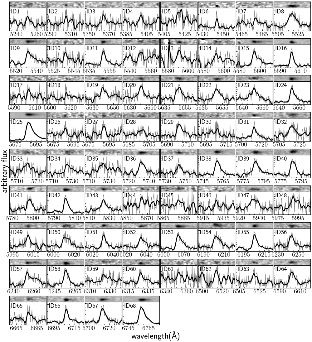
Figure 2: One- and two-dimensional spectra of all $g$-dropout galaxies showing Ly$\alpha$ emission lines. The object IDs are indicated in the upper left corner (column 1 of Table 1). The gray and black one-dimensional spectra are raw and smoothed by a Gaussian with the spectral resolution as width, respectively. The dispersion is $0.44\,\mathrm{\text{\AA}\,pixel^{-1}}$ while the spectral resolution is $\Delta\lambda=2.8\,\text{\AA}$.

We successfully identified emission lines from 68 galaxies among 210 spectroscopic targets. Most emission lines are skewed redward, which is a clear spectroscopic signature of Ly$\alpha$ emission from high-redshift galaxies (Figure 2). Such a skewed line profile can be quantified by weighted skewness, $S_{w}$ (Kashikawa et al., 2006), and most emission lines are high, positive values. No doublet like [O ii] emission was identified, in spite of sufficient spectral resolution to detect it if present (in which case the respective source would have been a low-redshift interloper). Considering alternative low-redshift interlopers, the wide spectral coverage of DEIMOS would enable detection of multiple emission lines if they were H$\beta$ or [O iii]. Therefore, all single emission lines are regarded as Ly$\alpha$ emission. Table 1 summarises the spectroscopic properties of the 68 confirmed galaxies. As the UV continuum of most of our targets is too faint to be detected by our spectroscopy, UV absolute magnitude ($M_{\mathrm{UV}}$) and Ly$\alpha$ equivalent width in the rest frame ($EW_{0}$) are calculated by using $i$-band photometry with the assumption of a flat UV continuum ($f_{\lambda}\propto\lambda^{\beta}$, where $\beta=-2$). As for brightest $g$-dropout galaxies ($m_{i}\lesssim 23.5$; ID15 and ID25), their UV continuum can be detected with a signal-to-noise ratio of $S/N\sim 2\mathrm{-}3$ by our spectroscopy. Due to this low $S/N$, we derive UV magnitude based on the broad-band photometry, even for such bright galaxies. Slit losses are assessed by using a bright star also observed within the same mask for calibration.

3 Results

3.1 Protocluster confirmation

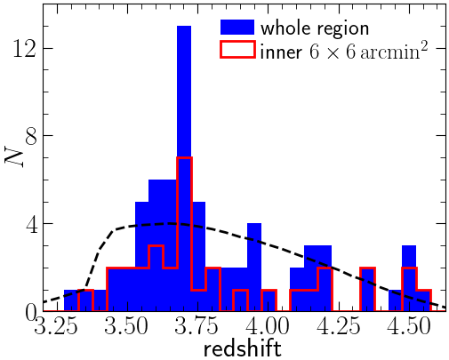
Figure 3: Redshift distribution of spectroscopically-confirmed galaxies. The red line shows the subset of galaxies located near the peak in surface overdensity. The black dashed line indicates the selection function of $g$-dropout galaxies, which is scaled to the number of spectroscopically-confirmed $g$-dropout galaxies. There is a clear redshift peak at $z=3.699$.

The redshift distribution of spectroscopically-confirmed galaxies exhibits a clear peak at $z=3.699$, including thirteen galaxies within $\Delta z<0.05$ (Figure 3). Based on the redshift window of $g$-dropout galaxies, the expected number of galaxies in the redshift bin of $\Delta z=0.05$ is $N\sim 4$. According to Poisson statistics for such a small sample size (Gehrels, 1986), the probability of more than thirteen galaxies clustering in such a narrow bin is only $<0.5\%$ by chance. Therefore, the thirteen galaxies are expected to be physically associated and form a genuine structure.

Table 1: Properties of spectroscopically-confirmed $g$-dropout galaxies.

ID	R.A.	Decl.	$m_{i}$	Redshift	$M_{\mathrm{UV}}$	$f_{\mathrm{Ly\alpha}}$	$L_{\mathrm{Ly\alpha}}$	$EW_{0}$	$S_{w}$
	(J2000)	(J2000)	(mag)		(mag)	($10^{-18}\,\mathrm{erg\,s^{-1}\,cm^{-2}}$)	($10^{42}\,\mathrm{erg\,s^{-1}}$)	(Å)	(Å)
1	10:01:39.87	+02:28:02.7	$26.99\pm 0.13$	$3.319\pm 0.001$	$-18.41\pm 0.23$	$3.78\pm 1.34$	$0.37\pm 0.13$	$18.3\pm 7.8$	$3.0\pm 1.5$
2	10:01:10.42	+02:28:25.9	$26.17\pm 0.06$	$3.363\pm 0.001$	$-19.36\pm 0.11$	$1.91\pm 1.65$	$0.19\pm 0.17$	$4.0\pm 3.5$	$3.6\pm 3.5$
3	10:01:00.45	+02:26:55.5	$24.87\pm 0.02$	$3.412\pm 0.001$	$-19.90\pm 0.07$	$2.41\pm 1.47$	$0.25\pm 0.15$	$3.2\pm 1.9$	$7.3\pm 6.2$
4	10:01:16.41	+02:26:44.3	$26.48\pm 0.08$	$3.441\pm 0.001$	$-19.16\pm 0.13$	$2.72\pm 1.82$	$0.29\pm 0.20$	$7.2\pm 4.9$	$0.0\pm 20.9$
5	10:01:07.96	+02:29:23.7	$26.05\pm 0.05$	$3.457\pm 0.001$	$-19.43\pm 0.10$	$3.79\pm 1.49$	$0.41\pm 0.16$	$7.9\pm 3.2$	$10.5\pm 7.9$
6	10:01:014.9	+02:29:29.9	$26.36\pm 0.07$	$3.478\pm 0.001$	$-19.18\pm 0.13$	$2.78\pm 0.85$	$0.31\pm 0.09$	$7.4\pm 2.5$	$2.7\pm 1.5$
7	10:01:08.22	+02:26:37.1	$25.23\pm 0.02$	$3.505\pm 0.001$	$-20.45\pm 0.04$	$1.90\pm 1.11$	$0.21\pm 0.13$	$1.6\pm 0.9$	$2.8\pm 2.0$
8	10:01:39.08	+02:27:37.0	$24.80\pm 0.02$	$3.540\pm 0.001$	$-20.91\pm 0.03$	$15.80\pm 2.75$	$1.81\pm 0.32$	$8.9\pm 1.6$	$3.4\pm 5.5$
9	10:01:49.05	+02:28:53.0	$24.47\pm 0.01$	$3.550\pm 0.001$	$-21.33\pm 0.02$	$26.36\pm 2.83$	$3.05\pm 0.33$	$10.2\pm 1.1$	$7.0\pm 1.2$
10	10:01:35.26	+02:27:10.7	$26.95\pm 0.12$	$3.554\pm 0.001$	$-18.60\pm 0.22$	$2.52\pm 1.28$	$0.29\pm 0.15$	$12.0\pm 6.7$	$2.0\pm 2.1$
11	10:01:19.07	+02:31:04.8	$27.03\pm 0.13$	$3.564\pm 0.001$	$-19.01\pm 0.16$	$10.72\pm 1.51$	$1.25\pm 0.18$	$35.2\pm 7.5$	$4.8\pm 1.8$
12	10:01:20.24	+02:28:00.4	$24.37\pm 0.01$	$3.566\pm 0.001$	$-21.01\pm 0.03$	$3.91\pm 1.50$	$0.46\pm 0.18$	$2.0\pm 0.8$	$3.6\pm 2.3$
13	10:01:40.26	+02:30:19.1	$25.95\pm 0.05$	$3.599\pm 0.001$	$-19.56\pm 0.10$	$5.30\pm 1.87$	$0.63\pm 0.22$	$10.7\pm 3.9$	$3.1\pm 2.9$
14	10:01:28.48	+02:29:00.5	$25.37\pm 0.03$	$3.600\pm 0.001$	$-20.35\pm 0.05$	$3.97\pm 1.31$	$0.48\pm 0.16$	$3.9\pm 1.3$	$1.8\pm 1.8$
15	10:01:32.12	+02:31:18.8	$23.29\pm 0.00$	$3.602\pm 0.001$	$-22.29\pm 0.01$	$26.05\pm 2.59$	$3.12\pm 0.31$	$4.3\pm 0.4$	$6.4\pm 1.1$
16	10:01:23.41	+02:29:34.8	$26.77\pm 0.10$	$3.608\pm 0.001$	$-19.10\pm 0.15$	$26.09\pm 2.01$	$3.14\pm 0.24$	$81.4\pm 14.0$	$4.7\pm 1.5$
17	10:00:59.22	+02:28:13.0	$25.98\pm 0.05$	$3.609\pm 0.001$	$-19.19\pm 0.14$	$1.47\pm 0.91$	$0.18\pm 0.11$	$4.2\pm 2.7$	$2.7\pm 2.2$
18	10:01:13.15	+02:28:11.5	$25.37\pm 0.03$	$3.619\pm 0.001$	$-20.30\pm 0.05$	$1.80\pm 1.12$	$0.22\pm 0.14$	$1.9\pm 1.2$	$1.3\pm 1.0$
19	10:01:52.54	+02:30:38.7	$25.41\pm 0.03$	$3.640\pm 0.001$	$-20.39\pm 0.05$	$5.36\pm 1.37$	$0.66\pm 0.17$	$5.2\pm 1.3$	$4.7\pm 2.5$
20	10:01:27.07	+02:29:33.1	$26.28\pm 0.07$	$3.640\pm 0.001$	$-19.73\pm 0.09$	$12.34\pm 3.12$	$1.52\pm 0.38$	$22.1\pm 5.9$	$3.4\pm 2.8$
21	10:01:05.63	+02:29:02.1	$25.15\pm 0.02$	$3.647\pm 0.001$	$-20.68\pm 0.04$	$14.65\pm 2.10$	$1.81\pm 0.26$	$10.9\pm 1.6$	$3.9\pm 1.4$
22	10:01:10.11	+02:29:06.1	$27.02\pm 0.13$	$3.647\pm 0.001$	$-18.80\pm 0.21$	$9.63\pm 1.87$	$1.19\pm 0.23$	$40.8\pm 11.7$	$3.2\pm 2.2$
23	10:01:00.06	+02:27:04.8	$25.79\pm 0.04$	$3.649\pm 0.001$	$-20.25\pm 0.06$	$11.03\pm 1.67$	$1.36\pm 0.21$	$12.3\pm 2.0$	$3.1\pm 1.5$
24	10:00:56.45	+02:29:42.0	$25.70\pm 0.04$	$3.650\pm 0.001$	$-20.14\pm 0.07$	$36.02\pm 2.87$	$4.45\pm 0.36$	$44.4\pm 4.5$	$7.5\pm 0.8$
25	10:01:45.73	+02:28:44.8	$23.53\pm 0.01$	$3.678\pm 0.001$	$-22.13\pm 0.01$	$123.72\pm 3.43$	$15.58\pm 0.43$	$24.9\pm 0.7$	$15.1\pm 0.6$
26	10:01:07.53	+02:29:21.1	$27.01\pm 0.13$	$3.678\pm 0.001$	$-18.64\pm 0.24$	$3.15\pm 1.53$	$0.40\pm 0.19$	$15.7\pm 8.6$	$0.6\pm 1.7$
27	10:00:55.94	+02:29:59.1	$26.02\pm 0.05$	$3.680\pm 0.001$	$-19.66\pm 0.10$	$2.29\pm 1.33$	$0.29\pm 0.17$	$4.5\pm 2.6$	$3.3\pm 18.6$
28	10:01:21.77	+02:28:22.3	$26.78\pm 0.10$	$3.686\pm 0.001$	$-18.80\pm 0.21$	$3.58\pm 1.24$	$0.45\pm 0.16$	$15.6\pm 6.4$	$0.7\pm 1.9$
29	10:01:41.81	+02:28:01.3	$25.40\pm 0.03$	$3.690\pm 0.001$	$-20.23\pm 0.06$	$7.20\pm 1.55$	$0.91\pm 0.20$	$8.4\pm 1.9$	$9.3\pm 3.5$
30	10:01:52.92	+02:28:24.3	$24.80\pm 0.02$	$3.693\pm 0.001$	$-20.82\pm 0.04$	$1.78\pm 1.04$	$0.23\pm 0.13$	$1.2\pm 0.7$	$-0.9\pm 2.2$
31	10:01:07.62	+02:28:53.5	$26.25\pm 0.06$	$3.699\pm 0.001$	$-19.55\pm 0.11$	$11.99\pm 1.27$	$1.53\pm 0.16$	$26.3\pm 4.0$	$3.8\pm 0.7$
32	10:01:26.43	+02:26:46.0	$24.62\pm 0.01$	$3.703\pm 0.001$	$-21.17\pm 0.03$	$8.56\pm 2.28$	$1.10\pm 0.29$	$4.2\pm 1.1$	$4.1\pm 3.4$
33	10:01:042.3	+02:29:05.5	$26.68\pm 0.09$	$3.705\pm 0.001$	$-19.27\pm 0.15$	$4.83\pm 1.77$	$0.62\pm 0.23$	$13.8\pm 5.4$	$1.8\pm 1.7$
34	10:01:29.14	+02:26:51.5	$25.23\pm 0.03$	$3.708\pm 0.001$	$-20.63\pm 0.04$	$9.03\pm 2.62$	$1.16\pm 0.34$	$7.4\pm 2.2$	$3.2\pm 1.6$
35	10:01:25.02	+02:26:51.6	$24.94\pm 0.02$	$3.708\pm 0.001$	$-20.74\pm 0.04$	$4.72\pm 1.68$	$0.61\pm 0.22$	$3.5\pm 1.2$	$1.3\pm 3.5$
36	10:01:24.86	+02:30:48.0	$26.26\pm 0.06$	$3.715\pm 0.001$	$-19.82\pm 0.09$	$20.89\pm 2.42$	$2.69\pm 0.31$	$36.0\pm 5.2$	$6.9\pm 1.3$
37	10:01:55.71	+02:30:17.2	$27.07\pm 0.14$	$3.724\pm 0.001$	$-18.94\pm 0.20$	$6.95\pm 1.53$	$0.90\pm 0.20$	$27.1\pm 8.0$	$4.0\pm 1.1$
38	10:01:020.7	+02:26:41.3	$26.13\pm 0.06$	$3.737\pm 0.001$	$-19.96\pm 0.08$	$31.06\pm 2.59$	$4.06\pm 0.34$	$47.8\pm 5.5$	$8.7\pm 1.1$
39	10:01:01.45	+02:28:51.1	$24.85\pm 0.02$	$3.759\pm 0.001$	$-20.87\pm 0.04$	$22.04\pm 2.60$	$2.92\pm 0.34$	$14.8\pm 1.8$	$7.9\pm 1.2$
40	10:01:00.34	+02:27:59.8	$24.32\pm 0.01$	$3.759\pm 0.001$	$-21.41\pm 0.02$	$33.57\pm 3.12$	$4.45\pm 0.41$	$13.8\pm 1.3$	$7.8\pm 1.3$
41	10:01:37.51	+02:27:32.9	$27.13\pm 0.14$	$3.767\pm 0.001$	$-18.86\pm 0.22$	$7.11\pm 1.66$	$0.95\pm 0.22$	$30.7\pm 9.9$	$2.3\pm 1.2$
42	10:01:37.21	+02:29:04.1	$26.54\pm 0.08$	$3.772\pm 0.001$	$-19.40\pm 0.14$	$18.22\pm 1.45$	$2.44\pm 0.19$	$48.2\pm 7.6$	$6.9\pm 1.3$
43	10:01:24.02	+02:29:12.8	$26.67\pm 0.09$	$3.791\pm 0.001$	$-19.44\pm 0.14$	$12.37\pm 2.41$	$1.67\pm 0.33$	$31.9\pm 7.6$	$4.1\pm 1.3$
44	10:01:29.59	+02:27:00.4	$26.74\pm 0.10$	$3.824\pm 0.001$	$-19.31\pm 0.16$	$1.52\pm 1.17$	$0.21\pm 0.16$	$4.5\pm 3.5$	$5.0\pm 8.9$
45	10:01:34.77	+02:27:41.0	$24.57\pm 0.01$	$3.837\pm 0.001$	$-21.33\pm 0.03$	$4.83\pm 1.59$	$0.67\pm 0.22$	$2.2\pm 0.7$	$1.1\pm 2.1$
46	10:00:046.8	+02:27:23.7	$26.24\pm 0.06$	$3.876\pm 0.001$	$-19.08\pm 0.20$	$2.60\pm 0.94$	$0.37\pm 0.13$	$9.8\pm 4.1$	$3.8\pm 1.7$
47	10:01:11.29	+02:28:34.2	$25.73\pm 0.04$	$3.882\pm 0.001$	$-19.95\pm 0.10$	$14.01\pm 2.49$	$2.01\pm 0.36$	$23.8\pm 4.8$	$8.7\pm 3.6$
48	10:00:50.25	+02:29:41.5	$25.79\pm 0.04$	$3.926\pm 0.001$	$-20.15\pm 0.08$	$7.14\pm 2.01$	$1.05\pm 0.30$	$10.3\pm 3.0$	$6.5\pm 3.8$
49	10:00:52.04	+02:27:57.1	$26.89\pm 0.11$	$3.943\pm 0.001$	$-19.29\pm 0.18$	$11.27\pm 1.58$	$1.67\pm 0.24$	$36.4\pm 8.3$	$4.9\pm 1.0$
50	10:01:02.44	+02:28:52.8	$26.17\pm 0.06$	$3.945\pm 0.001$	$-19.57\pm 0.14$	$9.81\pm 2.65$	$1.46\pm 0.39$	$24.5\pm 7.5$	$7.4\pm 4.5$
51	10:00:58.28	+02:29:12.3	$27.20\pm 0.15$	$3.961\pm 0.001$	$-18.82\pm 0.27$	$8.55\pm 1.47$	$1.28\pm 0.22$	$43.3\pm 14.4$	$3.3\pm 2.1$
52	10:01:35.74	+02:28:01.0	$27.18\pm 0.15$	$3.964\pm 0.001$	$-18.73\pm 0.29$	$6.69\pm 1.59$	$1.01\pm 0.24$	$36.9\pm 14.4$	$2.7\pm 1.8$
53	10:01:12.79	+02:27:40.4	$24.78\pm 0.02$	$3.989\pm 0.001$	$-21.14\pm 0.04$	$32.40\pm 2.70$	$4.95\pm 0.41$	$19.7\pm 1.8$	$8.9\pm 1.8$
54	10:01:06.75	+02:27:11.1	$26.63\pm 0.09$	$4.102\pm 0.001$	$-19.61\pm 0.16$	$18.10\pm 2.89$	$2.95\pm 0.47$	$48.0\pm 11.0$	$9.5\pm 3.9$
55	10:01:04.92	+02:29:18.6	$26.37\pm 0.07$	$4.104\pm 0.001$	$-19.68\pm 0.15$	$20.20\pm 1.76$	$3.30\pm 0.29$	$50.3\pm 8.8$	$6.8\pm 0.8$
56	10:01:46.84	+02:30:55.3	$26.26\pm 0.06$	$4.136\pm 0.001$	$-19.94\pm 0.13$	$18.28\pm 3.52$	$3.04\pm 0.59$	$36.7\pm 8.5$	$5.7\pm 2.5$
57	10:01:14.63	+02:31:21.1	$24.54\pm 0.01$	$4.144\pm 0.001$	$-21.43\pm 0.03$	$14.81\pm 2.02$	$2.48\pm 0.34$	$7.5\pm 1.1$	$5.0\pm 1.3$
58	10:01:33.76	+02:27:32.1	$26.60\pm 0.09$	$4.146\pm 0.001$	$-19.56\pm 0.18$	$15.44\pm 1.88$	$2.58\pm 0.32$	$43.8\pm 9.4$	$7.6\pm 1.7$
59	10:01:00.94	+02:27:41.8	$25.84\pm 0.04$	$4.201\pm 0.001$	$-20.48\pm 0.08$	$2.91\pm 1.05$	$0.50\pm 0.18$	$3.7\pm 1.4$	$2.4\pm 1.5$
60	10:01:15.88	+02:29:49.4	$27.01\pm 0.13$	$4.205\pm 0.001$	$-19.59\pm 0.18$	$5.67\pm 1.30$	$0.98\pm 0.22$	$16.3\pm 4.8$	$3.7\pm 3.0$
61	10:01:15.39	+02:27:08.6	$27.04\pm 0.13$	$4.225\pm 0.001$	$-19.33\pm 0.23$	$2.13\pm 1.20$	$0.37\pm 0.21$	$7.8\pm 4.8$	$1.3\pm 1.6$
62	10:01:22.81	+02:29:17.5	$25.11\pm 0.02$	$4.358\pm 0.001$	$-21.45\pm 0.04$	$3.08\pm 1.07$	$0.58\pm 0.20$	$1.7\pm 0.6$	$4.1\pm 5.9$
63	10:01:09.29	+02:26:50.6	$27.56\pm 0.21$	$4.363\pm 0.001$	$-19.51\pm 0.24$	$2.72\pm 1.00$	$0.51\pm 0.19$	$9.2\pm 4.0$	$0.7\pm 1.0$

Table 2: continued

ID	R.A.	Decl.	$m_{i}$	Redshift	$M_{\mathrm{UV}}$	$f_{\mathrm{Ly\alpha}}$	$L_{\mathrm{Ly\alpha}}$	$EW_{0}$	$S_{w}$
	(J2000)	(J2000)	(mag)		(mag)	($10^{-18}\,\mathrm{erg\,s^{-1}\,cm^{-2}}$)	($10^{42}\,\mathrm{erg\,s^{-1}}$)	(Å)	(Å)
64	10:01:04.53	+02:29:00.2	$26.04\pm 0.05$	$4.431\pm 0.001$	$-20.35\pm 0.13$	$9.03\pm 1.87$	$1.77\pm 0.37$	$14.5\pm 3.5$	$4.9\pm 3.1$
65	10:01:22.47	+02:28:56.1	$26.95\pm 0.12$	$4.492\pm 0.001$	$-19.43\pm 0.30$	$5.25\pm 1.46$	$1.06\pm 0.30$	$20.4\pm 8.7$	$3.2\pm 1.4$
66	10:01:16.32	+02:29:28.7	$27.28\pm 0.16$	$4.517\pm 0.001$	$-19.43\pm 0.31$	$9.29\pm 1.14$	$1.90\pm 0.23$	$36.3\pm 13.0$	$4.6\pm 0.7$
67	10:01:38.96	+02:30:32.8	$26.52\pm 0.08$	$4.523\pm 0.001$	$-19.65\pm 0.27$	$13.85\pm 1.78$	$2.85\pm 0.37$	$44.4\pm 13.7$	$5.5\pm 3.4$
68	10:01:19.38	+02:29:39.5	$25.91\pm 0.05$	$4.559\pm 0.001$	$-20.49\pm 0.14$	$41.50\pm 1.62$	$8.69\pm 0.34$	$62.8\pm 9.0$	$7.5\pm 0.7$

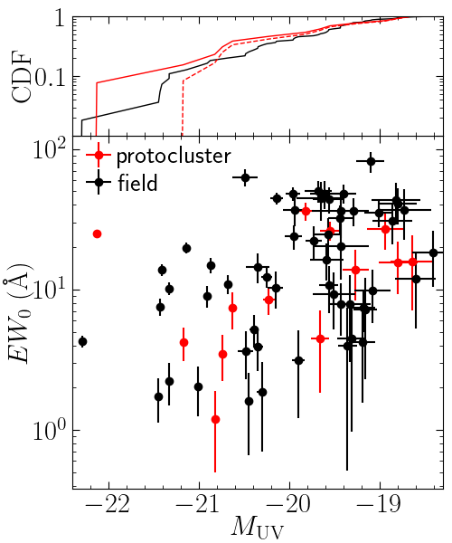
Figure 4: Physical properties of spectroscopically-confirmed $g$-dropout galaxies ($M_{\mathrm{UV}}$ and $EW_{0}$). The upper panel shows the cumulative distribution function (CDF) for protocluster and field galaxies. The dashed red line is derived by removing the brightest protocluster member, or AGN.

The structure at $z=3.699$ found by our spectroscopy is composed of thirteen galaxies at least, which is comparable to known protoclusters, and the galaxies are distributed over $\sim 12\,\mathrm{arcmin}$ corresponding to $\sim 5.2\,\mathrm{pMpc}$. The size of protoclusters is tightly correlated with the descendant halo mass at $z=0$ (Chiang et al., 2013; Muldrew et al., 2015). If our newly found structure is the progenitor of a rich cluster ($M_{h}>10^{15}\,\mathrm{M_{\sun}}$), the spatial distribution of its member galaxies at $z\sim 3\mathrm{-}4$ can indeed be expected to be on the order of $\sim 4\mathrm{-}6\,\mathrm{pMpc}$. On the other hand, considering the decreasing abundance of galaxy clusters with increasing mass, one may expect progenitors of typical galaxy clusters ($M_{h}\sim 10^{14}\,\mathrm{M_{\sun}}$) to be more frequently discovered than that of rich clusters. The size of the progenitors of such typical galaxy clusters is $\sim 2\mathrm{-}3\,\mathrm{pMpc}$. In contrast, previous studies confirmed several rich and large protoclusters: Lemaux et al. (2018) reported that nine spectroscopic protocluster members at $z=4.57$ are spread across an aperture of $\sim 6\,\mathrm{pMpc}$ diameter, a giant protocluster at $z=5.7$ having $\sim 5\,\mathrm{pMpc}$ size was found by Jiang et al. (2018), and a complex of protoclusters extending over $\sim 20\,\mathrm{pMpc}$ at $z=2.45$ was also discovered by Cucciati et al. (2018). Despite their rarity, it may be more feasible to confirm such rich protoclusters in actual observations. It should be noted that the shape of protoclusters at high redshifts is far from spherical, with filamentary elongations tracing the cosmic web (Lovell et al., 2018). Thus, the length of major axes of rich protoclusters can be $\sim 8\,\mathrm{pMpc}$. As shown in Figure 1, the overdense region of the ID4 protocluster candidate expands into the west and east directions. Since the FoVs of both DEIMOS masks were deliberately aligned with the elongation of the overdense region, wider coverage of the area surrounding the ID4 protocluster candidates (e.g., northern and southern parts) would be required in order to unbiasedly reveal the spatial distribution of member galaxies. Although it is difficult to draw a clear conclusion on its descendant structure at $z=0$, the thirteen galaxies clustering at $z=3.699$ can be regarded as a protocluster, possibly the progenitor of a rich cluster.

3.2 Galaxy properties

We next compare the galaxy properties between the thirteen protocluster members and field galaxies. As the field galaxies are identified as foreground/background galaxies from the same spectroscopic observation, there is less observational bias between the two samples. As shown in Figure 4, the overall trend of $M_{\mathrm{UV}}$ and $EW_{0}$ of protocluster members is not significantly different from that of field counterparts. That is, dropout galaxies with brighter UV magnitudes tend to have smaller $EW_{0}$ on average, regardless of their protocluster or field status. Such a trend is generally interpreted as more massive (and therefore brighter) SFGs being dustier, making it harder for the Ly$\alpha$ emission to escape. The fact that Ly$\alpha$ suffers more from dust attenuation than the UV continuum stems from its resonant scattering nature (see, e.g., Verhamme et al., 2006; Blaizot et al., 2023, for a discussion on Ly$\alpha$ radiative transfer).

In detail, some signs are present that set the protocluster members apart from field galaxies, especially at the bright end of the UV luminosity distribution. The fraction of particularly bright galaxies ($M_{\mathrm{UV}}<-22$) is only $\sim 0.02$ in the field; nevertheless, one of the thirteen protocluster members has such brightness. Given the bright-galaxy fraction of 0.02 ($1/55$) derived from field galaxies, the expected number of bright galaxies among the thirteen protocluster members is $0.24\pm 0.23$ according to a binomial distribution. This tendency of a relatively more populated UV-luminous end was already suggested by the photometric study of Toshikawa et al. (2024), and the follow-up spectroscopy shows a consistent result. This implies that there is no significant difference between the fraction of Ly$\alpha$ emitters among dropout galaxies in the protocluster and the field. Moreover, we note that in this case the brightest protocluster member deviates from the general relation between $M_{\mathrm{UV}}$ and $EW_{0}$, and its Ly$\alpha$ emission is found not only to be intense but also broad as shown in the left panel of Figure 5. The full width at half maximum of its Ly$\alpha$ emission is $\mathrm{FWHM}=1.7\,\text{\AA}$ in the rest frame or $\mathrm{FWHM}=420\,\mathrm{km\,s^{-1}}$. The brightest protocluster member has another emission line at $\lambda\sim 7300\,\text{\AA}$, corresponding to $\sim 1560\,\text{\AA}$ in the rest frame. Its integrated $S/N$ over $\lambda_{\mathrm{rest}}=1550\mathrm{-}1575\,\text{\AA}$ is $S/N\sim 7$. Although this wavelength is slightly different from that of C iv emission ($\lambda=1549.05\,\text{\AA}$), the observed wavelength of Ly$\alpha$ or C iv emissions could be shifted from the galaxy’s systemic redshift due to galactic kinematics (see, e.g., Rankine et al., 2020). Furthermore, the kinematic state of the broad line region of AGNs can cause large line profile differences for high-ionisation lines like C iv from object to object, and some AGNs exhibit absorption features superposed on a broad C iv emission line. Strong OH sky lines around $\lambda\sim 7300\,\text{\AA}$ can also hamper accurate line profile measurement. Thus, the emission line at $\lambda\sim 7300\,\text{\AA}$ can be regarded as C iv emission. Both intense/broad Ly$\alpha$ emission and the higher order ionisation emission of C iv can be attributed to the presence of an active galactic nucleus (AGN). As for field galaxies, no clear AGN is found. The bright-end excess is ascribed to the AGN, though there is still a marginal excess around $M_{\mathrm{UV}}\sim-20.5\,\mathrm{mag}$ (the upper panel of Figure 4).

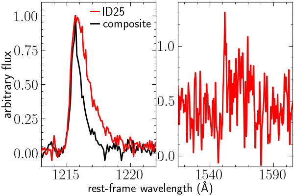
Figure 5: Spectrum of the brightest protocluster member zoomed in on Ly$\alpha$ and possible C iv emission in the left and right panels, respectively. For comparison, the composite Ly$\alpha$ emission line of the other $g$-dropout galaxies confirmed by the follow-up spectroscopy of this study are also plotted, enabling us to notice the broad Ly$\alpha$ emission of the brightest protocluster member.

In contrast to the brightest protocluster member, the other bright protocluster members tend to have smaller $EW_{0}$ than field galaxies. The median $\log(EW_{0}/\text{\AA})$ of protocluster members at $-22<M_{\mathrm{UV}}<-20$ is $\log(EW_{0}/\text{\AA})=0.63\pm 0.30$, compared to $\log(EW_{0}/\text{\AA})=0.98\pm 0.45$ for field counterparts. As Ly$\alpha$ emission is sensitive to dust attenuation, its strength relative to the UV continuum can be taken as a proxy for ISM maturity. The sense of the offset would then convey that brighter protocluster members may be more mature compared to field counterparts, albeit not at a statistically significant level. We have also checked the distribution of $EW_{0}$, and there is no significant difference between protocluster members and field galaxies ($p$-value of Kolmogorov-Smirnov test is $p=0.14$).

3.3 Protocluster structure

The three-dimensional (3D) distribution of protocluster members can be regarded as one of the key parameters marking the developmental phase of galaxy clusters and predictive of environmental effects on galaxy evolution. The evolution of size or internal structure of protoclusters are investigated by several theoretical works (e.g., Chiang et al., 2013; Muldrew et al., 2015; Lovell et al., 2018). As protoclusters are maturing, their shape, or the spatial distribution of member galaxies, tends to become more spherical, after an earlier developmental stage characterized by elongated or irregular shapes. In this study, a robust assessment of the shape of the protocluster is hampered by the limited FoV of our follow-up spectroscopy and the selection bias of protocluster members.

Here, we just calculate distance from the protocluster centre, $D_{\mathrm{cen}}$, and separation from the nearest neighbour, $D_{\mathrm{nei}}$, based on the thirteen spectroscopically-confirmed protocluster members. The protocluster centre is simply defined by the average position of protocluster members. This estimate of a centre assumes that Ly$\alpha$-emitting galaxies are unbiasedly distributed in the protocluster. Although it is quite difficult to directly check the validity of this assumption, Ly$\alpha$-emitting galaxies tend to be low-mass, young galaxies, implying that they are a major galaxy population in terms of number in a protocluster. We use redshifts as an indicator of line-of-sight distance as peculiar motions have only a minor effect on the observed redshifts. According to Henriques et al. (2015), the standard deviation of the difference between redshifts with and without peculiar motion is only $3.1\times 10^{-3}$ for $g$-dropout galaxies. Combined with the spectral resolution of our follow-up spectroscopy ($\mathrm{FWHM}=2.8\,\text{\AA}$ or $\delta z=9.8\times 10^{-4}$), the error in cosmological redshift is estimated to be $\delta z=3.3\times 10^{-3}$. This redshift uncertainty corresponds to $0.53\,\mathrm{pMpc}$. The error on the sky position (R.A. and Decl.) is negligible since the imaging dataset of HSC-SSP has a sufficiently high astrometric accuracy (standard deviation of $\sim 0.01\mathrm{-}0.02\,\mathrm{arcsec}$). We quantify the errors on the structural parameters $D_{\mathrm{cen}}$ and $D_{\mathrm{nei}}$ using Monte Carlo simulations. Specifically, the redshifts (line-of-sight distance) of protocluster members are perturbed according to a Gaussian distribution with $\sigma=3.3\times 10^{-3}$ ($0.53\,\mathrm{pMpc}$), and for each Monte Carlo realisation the structural parameters are calculated based on the perturbed redshifts. This process is repeated 10,000 times. The lower and upper errors are determined by the 16th and 84th percentiles, respectively. If redshift difference from the centre of the protocluster (the nearest neighbor) is almost zero, perturbing the redshift causes only larger separations. As for $D_{\mathrm{nei}}$, when a protocluster member is located near the middle of two other members, it is rare that $D_{\mathrm{nei}}$ becomes larger by perturbing redshifts. This explains the sometimes asymmetric error bars.

We show the relation between $D_{\mathrm{cen}}$ and $D_{\mathrm{nei}}$ in Figure 6. The estimate of the centre of the protocluster is less sensitive to the number of confirmed members, while the absolute separation from the nearest neighbor directly depends on the number density of confirmed members. If the completeness of our follow-up spectroscopy is uniform over the FoV, the separation from the nearest neighbour is still meaningful from a relative viewpoint. Protocluster members near the centre tend to have smaller $D_{\mathrm{nei}}$ ($\rho=0.59$ and $p=0.03$ based on the Spearman’s rank-order correlation test). Although observational biases (e.g., FoV of MOS masks and completeness) could have a significant effect on the measurement of 3D structure, the positive correlation between $D_{\mathrm{cen}}$ and $D_{\mathrm{nei}}$ indicates a centrally concentrated distribution of protocluster members. Strong substructure with galaxy groups falling onto one another would leave a lesser correlation (see, e.g., Toshikawa et al., 2020, for an example).

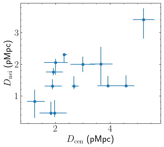
Figure 6: Relation between $D_{\mathrm{cen}}$ and $D_{\mathrm{nei}}$ (distance to protocluster centre and to closest other protocluster member) of thirteen protocluster members.

4 Discussion

4.1 Environmental dependence of galaxy properties

Informed by the above results on galaxy properties and 3D structure of the protocluster, we now discuss the relation between galaxy evolution and cluster formation. Figure 7 shows the relations between structural parameters ($D_{\mathrm{cen}}$ and $D_{\mathrm{nei}}$) and galaxy properties ($M_{\mathrm{UV}}$ and $EW_{0}$). There are tight correlations between $D_{\mathrm{nei}}$ and galaxy properties while $D_{\mathrm{cen}}$ is weakly correlated. The correlation coefficient and $p$-value for $D_{\mathrm{nei}}$ and $M_{\mathrm{UV}}$ ($EW_{0}$) are $\rho=0.74$ (0.81) and $p<0.01$, those for $D_{\mathrm{cen}}$ are $\rho=0.54$ (0.43) and $p=0.07$ (0.16). Here, we excluded the AGN (blue point) from the analysis because the physical mechanism of its strong UV/Ly$\alpha$ emission is entirely different from that in normal star-forming galaxies. Considering the fact that $D_{\mathrm{cen}}$ and $D_{\mathrm{nei}}$ are correlated among themselves, it cannot be denied that $D_{\mathrm{cen}}$ and galaxy properties are indirectly correlated through $D_{\mathrm{nei}}$.

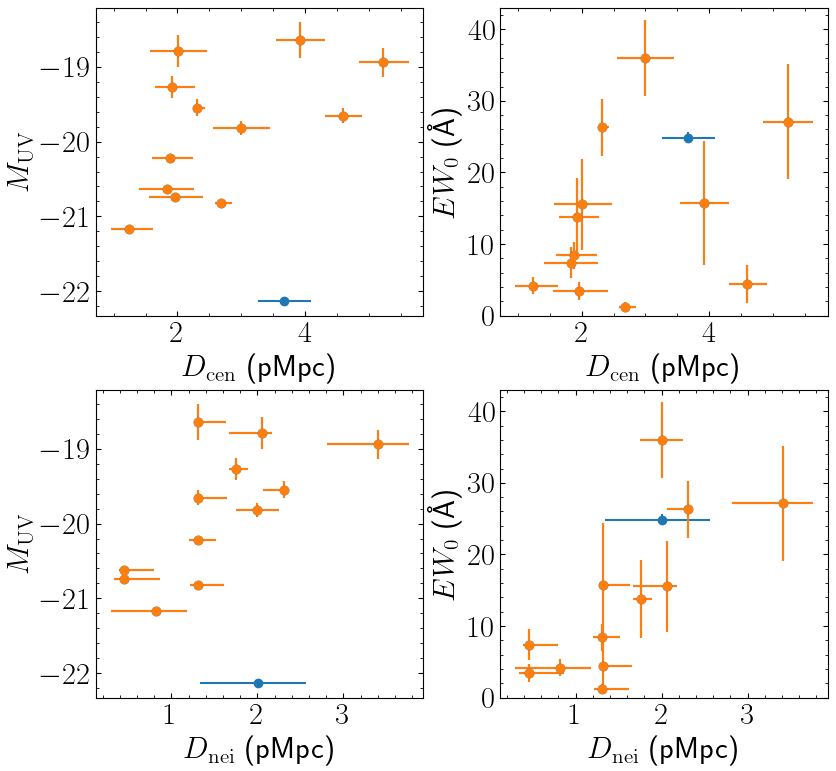
Figure 7: Relations between structural parameters (top panels for $D_{\mathrm{cen}}$, and bottom ones for $D_{\mathrm{nei}}$) and galaxy properties (left panels for $M_{\mathrm{UV}}$, and right ones for Ly$\alpha$ $EW_{0}$). The AGN is represented by blue points.

These results can be interpreted as the protocluster still being in an early phase of cluster formation where individual members are dependent on their local environments rather than the global structure of their host protocluster. This supports a hierarchical, or bottom-up, picture for structure formation. Protoclusters still experience drag from cosmic expansion and their physical size is increasing; thus, at high redshifts, protocluster members can have a physical connection only with their close neighbours. Smaller $D_{\mathrm{nei}}$, or higher local density, could result in a larger amount of gas accretion and/or more frequent galaxy mergers, and galaxy evolution or star-forming activity is enhanced as expected by brighter UV magnitude. Similarly, a reversal of the SFR-density relation at high redshifts ($2\lesssim z\lesssim 5$) is reported by several works (e.g., Lemaux et al., 2022; Taamoli et al., 2023; Shi et al., 2024). Although this study cannot reveal the underlying physical mechanism, it illustrates the apparent relation between environments and galaxy properties is dependent on the choice of the environmental indicator used since environmental effects on galaxy evolution, in general, involve a wide range of physics not only for enhancing but also quenching star-forming activity (e.g., Somerville & Davé, 2015; Alberts & Noble, 2022).

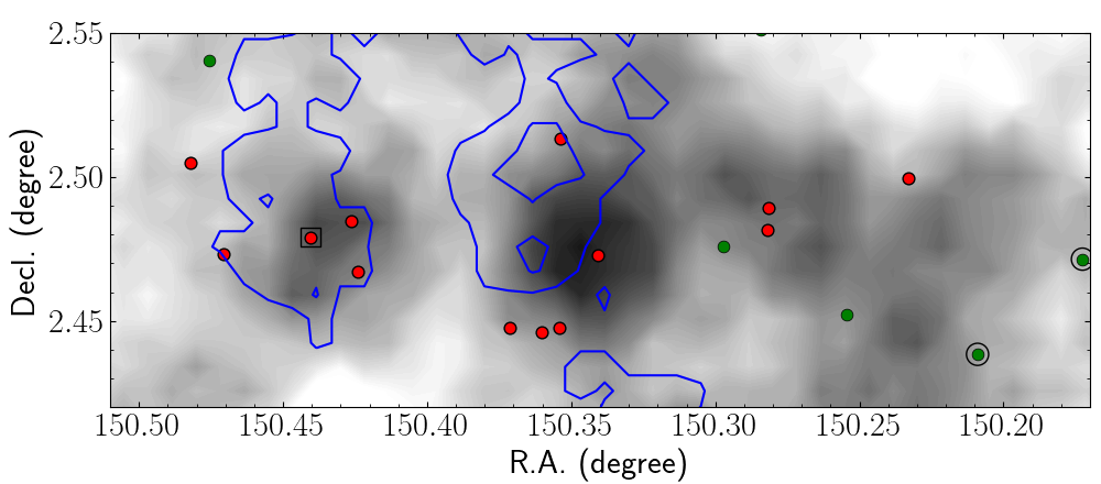
Figure 8: Overdensity map of $g$-dropout galaxies (grayscales) and the sky distribution of confirmed protocluster members (red circles) as shown in Figure 1. In addition, the blue lines are the ($2\sigma$ and $4\sigma$) overdensity contours of massive galaxies selected from COSMOS2020, and the green points are dusty star-burst galaxies from the COSMOS Super-deblended catalogue. The AGN and super-deblended sources with spectroscopic redshifts are shown by black square and circles, respectively.

The environment indicator of $D_{\mathrm{nei}}$ traces a relatively smaller scale than $D_{\mathrm{cen}}$; however, it cannot distinguish an isolated galaxy from a post-merger galaxy despite the fact that the underlying physical situations are completely different. The presence of an AGN in the protocluster may provide a clue on this. If AGN activity is triggered by galaxy mergers (e.g., Hopkins et al., 2008; Byrne-Mamahit et al., 2024), one may expect on statistical grounds that the AGN would most likely occur in the locally highest-density region in the protocluster. As illustrated in Figure 7, the AGN is located neither near the centre of the protocluster nor in the neighbourhood of smaller-$D_{\mathrm{nei}}$ galaxies. Instead, the location of the AGN is on the outskirt of the protocluster, which is a less probable outcome in a scenario where nuclear activity is triggered by mergers. Of course, AGNs being rare events and this study investigating only a single protocluster makes it hard to generalize any trends discerned. In another protocluster, discovered at $z=3.721$ following the same method as employed here, Toshikawa et al. (2020) found the single AGN presents to be located in the central part of the protocluster for example. Noirot et al. (2018) confirmed 16 protoclusters by targeting RGs as signposts, but RGs are not always located at the centre of the structures. Extending such investigation to other known protoclusters would lead to a more heterogeneous sample as they were discovered by various methods, thus hampering a fair comparison. The HSC-SSP provides a systematic sample of protocluster candidates across cosmic time (Toshikawa et al., 2018; Higuchi et al., 2019; Toshikawa et al., 2024). Combined with the campaign of follow-up spectroscopy, we will be able to draw a conclusion on the relation between protoclusters and rare objects like AGNs in the future.

4.2 Other galaxy populations

We have confirmed the correlation between $D_{\mathrm{nei}}$ and galaxy properties, indicating that locally high-density environments enhance star-forming activity. This can most plausibly be read as galaxy evolution being accelerated in dense environments, although an enhancement of starburst triggering may contribute as well. Our method relies on $g$-dropout galaxies, and thus focuses on the dust-poor star-forming galaxy population, even more so given that Ly$\alpha$ emission is needed to pinpoint the $g$-dropout galaxies in 3D space. Such selection may miss the most vigorous star-forming systems, which tend to be enshrouded by dust, or other objects with high mass-to-light ratios. Actually, some protoclusters even at $z\gtrsim 4$ are found to host massive quiescent galaxies (Tanaka et al., 2023; Kakimoto et al., 2024). In order to find relatively mature galaxies or starburst galaxies, if any, we make use of the public COSMOS2020 (Weaver et al., 2022) and Super-deblended (Jin et al., 2018) catalogues. Even a deep and well-sampled multiwavelength dataset such as available in the COSMOS field is unable to photometrically constrain redshifts with an accuracy equivalent to the redshift size of the protocluster ($\Delta z<0.05$). Therefore, we simply select galaxies whose best photometric redshifts are within the interval $3.675<z_{\mathrm{phot}}<3.725$, corresponding to the redshift range of the protocluster, irrespective of the size of their photo-z error. As the typical error is $\sigma_{z_{\mathrm{phot}}}\sim 0.7$ for $z\sim 3.7$ galaxies in the COSMOS2020 catalogue, it is meaningless to judge whether individual galaxies are protocluster members or not. However, despite the unavoidable dilution by interlopers, it remains useful to evaluate whether an enhancement of mature galaxies is present in the vicinity of the protocluster.

Relatively mature galaxies can be selected from the COSMOS2020 catalogue by $\log(M_{\mathrm{star}})>9.0$. This threshold accounts for about the upper half of more massive galaxies among all galaxies at $z_{\mathrm{phot}}\sim 3.7$. As there is a correlation between stellar mass and age, it is highly expected that more massive galaxies are equivalent to older, more mature galaxies. According to the CLASSIC catalogue with LePhare photometric redshifts, $N=1382$ galaxies are selected over the whole survey area of COSMOS2020, resulting in 2.4 such galaxies per 1$\aas@@fstack{\prime}$8-radius aperture on average. Having calculated the surface overdensity of these massive galaxies by the same method as we applied for $g$-dropout galaxies in Toshikawa et al. (2024), we find massive galaxies at $z=3.7$ to also show a high overdensity near the peak overdensity of $g$-dropout galaxies (Figure 8). This suggests that massive galaxies densely populate the core of the protocluster. It is not common for such mature galaxies to have strong Ly$\alpha$ emissions; thus, the lack of confirmed protocluster members within $D_{\mathrm{cen}}<1\,\mathrm{pMpc}$ (Figure 7) could be attributed to the observational bias of our follow-up spectroscopy, which entirely relies on the presence of (strong) Ly$\alpha$ emission. Although the existence of the protocluster was confirmed by our follow-up spectroscopy targeting Ly$\alpha$ (Section 3.1), the protocluster is expected to be composed of multiple galaxy populations based on the sky distribution of mature galaxies. Another interesting feature of the overdensity map of mature galaxies is that the eastern part of the protocluster shows moderate overdensity while there is no overdensity in the western part. The AGN also happens to be located in the eastern part. Perhaps, the eastern part is a subgroup falling into the main component of the protocluster.

The number of galaxies contained in the Super-deblended catalogue, which contains far-infrared photometry, is about a tenth of that in the COSMOS2020 catalogue. This is too scarce to measure overdensity. Thus, galaxies at $z=3.700\pm 0.025$ selected from the Super-deblended catalogue are just overplotted on the overdensity map of $g$-dropout galaxies in Figure 8. There are five galaxies around the protocluster, and they seem to be biased toward the western part. Their SFRs are inferred to be $\sim 250\mathrm{-}1200\,\mathrm{M_{\sun}\,yr^{-1}}$ from the combination of optical to far-infrared photometry and SED fitting technique, which is $\times 10\mathrm{-}100$ higher than the typical SFR of dropout galaxies. It should be noted that two of the five infrared-detected galaxies were already confirmed to be at $z=3.709$ and 3.710 by spectroscopy (Lilly et al., 2009; Tasca et al., 2017). Their redshifts are perfectly matched to the redshift range of the protocluster. The total SFR of these two Super-deblended sources with spectroscopic redshifts is $\sim 1000\,\mathrm{M_{\sun}\,yr^{-1}}$. Similar to the AGN, the dusty star-burst galaxies are located in the outskirts of the protocluster, provided that $g$-dropout (i.e., dust-poor star-forming) galaxies correctly trace the protocluster structure. It should be noted that there are some clear examples of protocluster cores composed of dusty star-burst galaxies at $z\sim 4$ (Miller et al., 2018; Oteo et al., 2018). Such dusty star-burst galaxies in a protocluster core are predicted to merge into a single massive galaxy like a Brightest Cluster Galaxy (BCG) as seen in the local universe (Rennehan et al., 2020). Interestingly, Rotermund et al. (2021) found that a protocluster core at $z=4.3$ composed of many dusty star-burst galaxies does not exhibit a high overdensity of dropout galaxies. Although it is difficult to determine which galaxy population is the better tracer of environments or cosmic structure, it is clear that steady galaxy evolution represented by dropout galaxies and stochastic phases like experienced by star-bursting objects can occur in (locally) different environments. The spatial segregation of galaxy populations makes it difficult to draw a conclusion on a protocluster’s structure.

5 Conclusions

We have presented the spectroscopic confirmation of a protocluster at $z=3.699$ in the HSC-DUD layer. This protocluster is composed of at least thirteen member galaxies. As indicated by the photometric data (Toshikawa et al., 2024), spectroscopically-confirmed protocluster members tend to be brighter in rest-frame UV than field counterparts. One of these bright protocluster members is serendipitously identified to be an AGN though our protocluster search does not depend on the presence of AGNs. In addition, protocluster structure is investigated in terms of galaxies’ separation from the centre of the protocluster, $D_{\mathrm{cen}}$, and from their nearest neighbours, $D_{\mathrm{nei}}$. The protocluster has a centrally-concentrated spatial distribution of member galaxies as indicated by a correlation between $D_{\mathrm{cen}}$ and $D_{\mathrm{nei}}$.

We next compared galaxy properties ($M_{\mathrm{UV}}$ and Ly$\alpha$ $EW_{0}$) with the spatial parameters $D_{\mathrm{cen}}$ and $D_{\mathrm{nei}}$. The galaxy properties $M_{\mathrm{UV}}$ and Ly$\alpha$ $EW_{0}$ are more tightly related to $D_{\mathrm{nei}}$. Since $M_{\mathrm{UV}}$ and Ly$\alpha$ $EW_{0}$ originate from strong radiation from massive stars, this suggests that star-forming activity is more sensitive to smaller-scale environments rather than the position within the overall protocluster. In addition to the presence of an AGN, the environmental enhancement of star-forming activity results in an overabundance of bright galaxies.

In order to search for other galaxy populations, that are not traced by the dropout technique, we have made use of the public dataset of the COSMOS2020 and Super-deblended catalogues in the COSMOS field. Massive, or mature, galaxies selected from the COSMOS2020 catalogue exhibit a higher overdensity near the centre of the protocluster, implying that the protocluster has a higher galaxy density at the centre than observed via Ly$\alpha$-emitting $g$-dropout galaxies. In contrast, dusty star-burst galaxies selected from the Super-deblended catalogue reside in the outskirts of the protocluster. Although it is beyond the scope of this study to reveal the physical origin of this spatial segregation depending on the galaxy population from star-burst to mature galaxies, our analysis demonstrates a complex of multiple galaxy populations even at $z=3.7$.

This paper reports follow-up spectroscopy on a protocluster candidate among $N\sim 100$ samples in the HSC-DUD layer, as a pilot observation. Even from this single case, we have obtained an insight into the relation between galaxy evolution and cluster formation. In the future, we will expand this campaign of follow-up spectroscopy to address the general trend and physical origin of the diversity of cluster formation.

Data Availability

The data underlying this article will be shared on reasonable request to the corresponding author.

References

- Aihara et al. (2018) Aihara H., et al., 2018, PASJ, 70, S4
- Alberts & Noble (2022) Alberts S., Noble A., 2022, Universe, 8, 554
- Alpaslan et al. (2014) Alpaslan M., et al., 2014, MNRAS, 438, 177
- Ayromlou et al. (2019) Ayromlou M., Nelson D., Yates R. M., Kauffmann G., White S. D. M., 2019, MNRAS, 487, 4313
- Barnes et al. (2017) Barnes D. J., et al., 2017, MNRAS, 471, 1088
- Blaizot et al. (2023) Blaizot J., et al., 2023, MNRAS, 523, 3749
- Byrne-Mamahit et al. (2024) Byrne-Mamahit S., Patton D. R., Ellison S. L., Bickley R., Ferreira L., Hani M., Quai S., Wilkinson S., 2024, MNRAS, 528, 5864
- Calvi et al. (2021) Calvi R., Dannerbauer H., Arrabal Haro P., Rodríguez Espinosa J. M., Muñoz-Tuñón C., Pérez González P. G., Geier S., 2021, MNRAS, 502, 4558
- Calvi et al. (2023) Calvi R., Castignani G., Dannerbauer H., 2023, A&A, 678, A15
- Casey (2016) Casey C. M., 2016, ApJ, 824, 36
- Chanchaiworawit et al. (2019) Chanchaiworawit K., et al., 2019, ApJ, 877, 51
- Chiang et al. (2013) Chiang Y.-K., Overzier R., Gebhardt K., 2013, ApJ, 779, 127
- Clements et al. (2016) Clements D. L., et al., 2016, MNRAS, 461, 1719
- Cucciati et al. (2018) Cucciati O., et al., 2018, A&A, 619, A49
- Daddi et al. (2022) Daddi E., et al., 2022, ApJ, 926, L21
- Douglas et al. (2010) Douglas L. S., Bremer M. N., Lehnert M. D., Stanway E. R., Milvang-Jensen B., 2010, MNRAS, 409, 1155
- Dressler (1980) Dressler A., 1980, ApJ, 236, 351
- Faber et al. (2003) Faber S. M., et al., 2003, in Iye M., Moorwood A. F. M., eds, Society of Photo-Optical Instrumentation Engineers (SPIE) Conference Series Vol. 4841, Instrument Design and Performance for Optical/Infrared Ground-based Telescopes. pp 1657–1669, doi:10.1117/12.460346
- Fumagalli et al. (2024) Fumagalli A., Costanzi M., Saro A., Castro T., Borgani S., 2024, A&A, 682, A148
- Gallazzi et al. (2021) Gallazzi A. R., Pasquali A., Zibetti S., Barbera F. L., 2021, MNRAS, 502, 4457
- Gao et al. (2022) Gao F., Wang L., Ramos Padilla A. F., Clements D., Farrah D., Huang T., 2022, A&A, 668, A54
- Gehrels (1986) Gehrels N., 1986, ApJ, 303, 336
- Ghirardini et al. (2024) Ghirardini V., et al., 2024, arXiv e-prints, p. arXiv:2402.08458
- Hatch et al. (2014) Hatch N. A., et al., 2014, MNRAS, 445, 280
- Henriques et al. (2015) Henriques B. M. B., White S. D. M., Thomas P. A., Angulo R., Guo Q., Lemson G., Springel V., Overzier R., 2015, MNRAS, 451, 2663
- Henriques et al. (2020) Henriques B. M. B., Yates R. M., Fu J., Guo Q., Kauffmann G., Srisawat C., Thomas P. A., White S. D. M., 2020, MNRAS, 491, 5795
- Higuchi et al. (2019) Higuchi R., et al., 2019, ApJ, 879, 28
- Hill et al. (2020) Hill R., et al., 2020, MNRAS, 495, 3124
- Hoessel et al. (1980) Hoessel J. G., Gunn J. E., Thuan T. X., 1980, ApJ, 241, 486
- Hopkins et al. (2008) Hopkins P. F., Hernquist L., Cox T. J., Kereš D., 2008, ApJS, 175, 356
- Ito et al. (2019) Ito K., et al., 2019, ApJ, 878, 68
- Ito et al. (2020) Ito K., et al., 2020, ApJ, 899, 5
- Ito et al. (2023) Ito K., et al., 2023, ApJ, 945, L9
- Jiang et al. (2018) Jiang L., et al., 2018, Nature Astronomy, 2, 962
- Jin et al. (2018) Jin S., et al., 2018, ApJ, 864, 56
- Kakimoto et al. (2024) Kakimoto T., et al., 2024, ApJ, 963, 49
- Kashikawa et al. (2006) Kashikawa N., et al., 2006, ApJ, 648, 7
- Kato et al. (2016) Kato Y., et al., 2016, MNRAS, 460, 3861
- Kubo et al. (2019) Kubo M., et al., 2019, ApJ, 887, 214
- Kubo et al. (2021) Kubo M., et al., 2021, ApJ, 919, 6
- Lemaux et al. (2018) Lemaux B. C., et al., 2018, A&A, 615, A77
- Lemaux et al. (2022) Lemaux B. C., et al., 2022, A&A, 662, A33
- Libeskind et al. (2018) Libeskind N. I., et al., 2018, MNRAS, 473, 1195
- Lilly et al. (2009) Lilly S. J., et al., 2009, ApJS, 184, 218
- Lovell et al. (2018) Lovell C. C., Thomas P. A., Wilkins S. M., 2018, MNRAS, 474, 4612
- Luo et al. (2022) Luo Y., et al., 2022, ApJ, 935, 80
- Matsuda et al. (2011) Matsuda Y., et al., 2011, MNRAS, 410, L13
- Miller et al. (2018) Miller T. B., et al., 2018, Nature, 556, 469
- Miyazaki et al. (2018) Miyazaki S., et al., 2018, PASJ, 70, S1
- Muldrew et al. (2015) Muldrew S. I., Hatch N. A., Cooke E. A., 2015, MNRAS, 452, 2528
- Nelson et al. (2023) Nelson D., Pillepich A., Ayromlou M., Lee W., Lehle K., Rohr E., Truong N., 2023, arXiv e-prints, p. arXiv:2311.06338
- Noirot et al. (2018) Noirot G., et al., 2018, ApJ, 859, 38
- Oteo et al. (2018) Oteo I., et al., 2018, ApJ, 856, 72
- Ouchi et al. (2005) Ouchi M., et al., 2005, ApJ, 620, L1
- Overzier (2016) Overzier R. A., 2016, A&ARv, 24, 14
- Peebles (1980) Peebles P. J. E., 1980, The large-scale structure of the universe
- Press & Schechter (1974) Press W. H., Schechter P., 1974, ApJ, 187, 425
- Prochaska et al. (2020) Prochaska J. X., et al., 2020, Journal of Open Source Software, 5, 2308
- Rankine et al. (2020) Rankine A. L., Hewett P. C., Banerji M., Richards G. T., 2020, MNRAS, 492, 4553
- Rennehan et al. (2020) Rennehan D., Babul A., Hayward C. C., Bottrell C., Hani M. H., Chapman S. C., 2020, MNRAS, 493, 4607
- Rotermund et al. (2021) Rotermund K. M., et al., 2021, MNRAS, 502, 1797
- Sawicki et al. (2019) Sawicki M., et al., 2019, MNRAS, 489, 5202
- Shi et al. (2020) Shi K., Toshikawa J., Cai Z., Lee K.-S., Fang T., 2020, ApJ, 899, 79
- Shi et al. (2021) Shi K., Toshikawa J., Lee K.-S., Wang T., Cai Z., Fang T., 2021, ApJ, 911, 46
- Shi et al. (2024) Shi K., Malavasi N., Toshikawa J., Zheng X., 2024, ApJ, 961, 39
- Somerville & Davé (2015) Somerville R. S., Davé R., 2015, ARA&A, 53, 51
- Springel et al. (2005) Springel V., et al., 2005, Nature, 435, 629
- Steidel et al. (1998) Steidel C. C., Adelberger K. L., Dickinson M., Giavalisco M., Pettini M., Kellogg M., 1998, ApJ, 492, 428
- Taamoli et al. (2023) Taamoli S., et al., 2023, arXiv e-prints, p. arXiv:2312.10222
- Tanaka et al. (2023) Tanaka M., et al., 2023, arXiv e-prints, p. arXiv:2311.11569
- Tasca et al. (2017) Tasca L. A. M., et al., 2017, A&A, 600, A110
- Toshikawa et al. (2012) Toshikawa J., et al., 2012, ApJ, 750, 137
- Toshikawa et al. (2016) Toshikawa J., et al., 2016, ApJ, 826, 114
- Toshikawa et al. (2018) Toshikawa J., et al., 2018, PASJ, 70, S12
- Toshikawa et al. (2020) Toshikawa J., Malkan M. A., Kashikawa N., Overzier R., Uchiyama H., Ota K., Ishikawa S., Ito K., 2020, ApJ, 888, 89
- Toshikawa et al. (2024) Toshikawa J., et al., 2024, MNRAS, 527, 6276
- Uchiyama et al. (2018) Uchiyama H., et al., 2018, PASJ, 70, S32
- Umehata et al. (2019) Umehata H., et al., 2019, Science, 366, 97
- Venemans et al. (2007) Venemans B. P., et al., 2007, A&A, 461, 823
- Verhamme et al. (2006) Verhamme A., Schaerer D., Maselli A., 2006, A&A, 460, 397
- Weaver et al. (2022) Weaver J. R., et al., 2022, ApJS, 258, 11
- Wen & Han (2013) Wen Z. L., Han J. L., 2013, MNRAS, 436, 275
- Wetzel et al. (2012) Wetzel A. R., Tinker J. L., Conroy C., 2012, MNRAS, 424, 232
- Wylezalek et al. (2013) Wylezalek D., et al., 2013, ApJ, 769, 79
- Yuan et al. (2022) Yuan Z. S., Han J. L., Wen Z. L., 2022, MNRAS, 513, 3013