Addendum to “Power-law decay of the fraction of the mixed eigenstates in kicked top model with mixed-type classical phase space”

Abstract

By using the Krylov subspace technique to generate the spin coherent states in kicked top model, a prototype model for studying quantum chaos, the accessible system size for studying the Husimi functions of eigenstates can be much larger than that reported in the literature and our previous study Phys. Rev. E 108, 054217 (2023). In the fully chaotic kicked top, we find that the mean Wehrl entropy localization measure approaches the prediction given by the Circular Unitary Ensemble. In the mixed-type case, we identify mixed eigenstates by the overlap of the Husimi function with regular and chaotic regions in classical compact phase space. Numerically, we show that the fraction of mixed eigenstates scales as $j^{-\zeta}$, a power-law decay as the system size $j$ increases, across nearly two orders of magnitude. This provides supporting evidence for the principle of uniform semiclassical condensation of Husimi functions and the Berry-Robnik picture in the semiclassical limit.

I Introduction

At the very beginning of quantum chaos it was Percival [1] who proposed to distinguish between the regular quantum eigenstates and the chaotic ones, associated with classical regular and chaotic regions in the phase space, respectively. They should be distinguished by the nature of their energy spectra, namely by their sensitivity with respect to small perturbations. This line of thought led to the semiclassical eigenfunction hypothesis by Berry [2], which is crucial for understanding quantum eigenstates. It proposes that in the semiclassical limit, quantum eigenstates concentrate on compact phase space regions explored by typical trajectories in the long time limit. In integrable systems, these are the invariant tori, while in ergodic dynamics, eigenstates equidistribute on the energy surface. In mixed-type systems with both regular and chaotic motions in phase space [3], eigenstates concentrate either on regular or chaotic regions. This hypothesis finally develops into the so-called principle of uniform semiclassical condensation (PUSC) of Wigner functions (or Husimi functions) [4]. This principle, in turn, directly leads to the eigenstate thermalization hypothesis conjecture by Srednicki [5], which is now recognized as an explanation for the emergence of thermodynamic equilibrium in isolated quantum many-body systems [6, 7, 8]. Moreover, as a consequence of this principle, the spectral statistics for regular and chaotic states in the semiclassical limit are separately described by Poissonian statistics [9] and random matrix theory [10, 11, 12], while the entire spectrum is effectively captured by the Berry-Robnik picture [13].

Regarding the behavior of quantum eigenstates in mixed-type systems away from the semiclassical limit, one expects various tunneling processes between different phase-space structures. Among these are the chaos-assisted tunneling between different regular regions [14, 15, 16], the flooding of chaotic states into regular islands [17], and the so-called resonance-assisted tunneling between the regular island across the chaotic sea [18, 19, 20, 21]. The general behavior of quantum states approaching the semiclassical limit is not well studied [22]. Through the overlap of the Husimi function with both regular and chaotic regions in classical compact phase space, mixed eigenstates can be identified, distinct from regular and fully chaotic states. Very recently, in quantum billiards [23], it was found that the fraction of mixed states shows a power-law decay as the semiclassical limit is approached, across two orders of magnitude. In quantum kicked top (QKT), a prototype Floquet model for studying quantum chaos [24, 25], our previous study [26] also showed a power-law decay for mixed-type QKT, but only within a relatively small range of system sizes. This limitation arises from our method used to generate the spin coherent state (SCS), where a direct calculation of large factorials are unavoidable.

In this addendum paper, we use the Krylov subspace techniques [27, 28, 29, 30] to generate the SCS and avoid the factorials. This allows for a significantly larger accessible system size for studying Husimi functions, compared to that reported in literature and our previous study. In the fully chaotic QKT, we find that the mean Wehrl entropy localization measure (ELM) approaches the prediction given by the Circular Unitary Ensemble (CUE). In the mixed-type case, we show a power-law decrease of the fraction of mixed eigenstates as system size increases over nearly two orders of magnitude, corroborating the PUSC and the Berry-Robnik picture in the semiclassical limit.

The paper is organized as follows. In Sec. II, we introduce QKT and analyze the transition to chaos for both its classical correspondence and quantum case. In Sec. III, we give the definition of the SCS and apply the Krylov subspace technique to generate them. We then establish a consistent transition to chaos using the mean Wehrl ELM, compared to other indicators of chaos. In the fully chaotic QKT, we study the mean Wehrl ELM versus the system size. In Sec. IV, we analyze the joint distribution of the phase-space overlap index and Wehrl ELM, and show as the system size increases, how the distribution of the former evolves, as well as the fraction of mixed states. We draw our conclusion in Sec. V.

II Quantum kicked top

The QKT is described by the Hamiltonian [24]

$$H=\alpha J_{x}+\frac{\gamma}{2j}J_{z}^{2}\sum_{n=-\infty}^{\infty}\delta(t-n),$$ (1)

where the dynamical variables of the top are three components of the angular momentum operators of the spin-$j$ system, can also be expressed in terms of $2j$ collective spin-$\frac{1}{2}$ Pauli operators, for example $J_{z}=\sum_{k=1}^{2j}\sigma_{z}^{(k)}/2$. The dimension of the Hilbert space is $N=2j+1$, and the squared angular momentum is conserved, $J^{2}=j(j+1)$ with $j$ integer or half-integer. The first term in Eq. (1) describes a precessional rotation about the $x$-axis with angular frequency $\alpha$, the second term denotes a torsional rotation around the $z$-axis with strength $\gamma$ (with the period set to unity).

The dynamical evolution of the QKT is governed by the Floquet operator

$$F=\exp(-i\frac{\gamma}{2j}J_{z}^{2})\exp(-i\alpha J_{x}),$$ (2)

is invariant under rotation by the angle $\pi$ along the $x$-axis $R_{x}=e^{i\pi J_{x}}$, which suggests the even or odd parity of the quasi-energy. Using this symmetry, the $(2j+1)$-dimensional unitary matrix $F$ in the representation of the Dicke states {$|j,m\rangle,|m|\leq j$}, i.e. eigenstates of $J_{z}$, can further be reduced to two unitary matrices

$$F_{m,m^{\prime}}^{\pm} =\langle j,m,\pm|F|j,m^{\prime},\pm\rangle,$$ (3)

where $|j,m,\pm\rangle=(|j,m\rangle\pm|j,-m\rangle)/\sqrt{2}$, $1\leq m\leq j$ for the odd parity, and $0\leq m\leq j$ for the even parity where $|j,0,+\rangle$ is not normalized. It should be noted that at $\alpha=\pi/2$, the QKT has a further symmetry [25]. In this addendum paper, we set $\alpha=11\pi/19$, the same as the previous work.

The Heisenberg equation of motion is given by the map $J_{i,n+1}=F^{\dagger}J_{i,n}F$, where $J_{i,n}\equiv J_{i}(n)$ denotes the time-evolved operators at $t=n$. Using Baker-Campbell-Hausdorff (BCH) formula for the expansion of the map, one has

$$J_{x,n+1} =\frac{1}{2}[\tilde{J}_{x,n}+i\tilde{J}_{y,n}]\exp\left[i\frac{\gamma}{2j}(2\tilde{J}_{z,n}+1)\right]+h.c.,$$

$$J_{y,n+1} =\frac{1}{2i}[\tilde{J}_{x,n}+i\tilde{J}_{y,n}]\exp\left[i\frac{\gamma}{2j}(2\tilde{J}_{z,n}+1)\right]+h.c,$$

$$J_{z,n+1} =\tilde{J}_{z,n},$$ (4)

where $\tilde{J}_{x,n}=J_{x,n}$, $\tilde{J}_{y,n}=J_{y,n}\cos\alpha-J_{z,n}\sin\alpha$, and $\tilde{J}_{z,n}=J_{y,n}\sin\alpha+J_{z,n}\cos\alpha$.

II.1 The transition to Hamiltonian chaos

The classical map emerges in the classical limit as $j\to\infty$ where noncummutivity is negligible and the rescaled Heisenberg operators $\mathbf{x}_{n}\equiv\mathbf{x}(n)=\mathbf{J}_{n}/j$ tend to a unit vector with commuting components. From Eq. (II), the classical equations of motion follow

$$x_{n+1} =\tilde{x}_{n}\cos\gamma\tilde{z}_{n}-\tilde{y}_{n}\sin\gamma\tilde{z}_{n},$$

$$y_{n+1} =\tilde{x}_{n}\sin\gamma\tilde{z}_{n}+\tilde{y}_{n}\cos\gamma\tilde{z}_{n},$$

$$z_{n+1} =\tilde{z}_{n},$$ (5)

where $\tilde{x}_{n}=x_{n}$, $\tilde{y}_{n}=y_{n}\cos\alpha-z_{n}\sin\alpha$, and $\tilde{z}_{n}=y_{n}\sin\alpha+z_{n}\cos\alpha$. This classical map $\mathbf{x}_{n+1}=f(\mathbf{x}_{n})$ is restricted on the unit sphere $\mathbb{S}^{2}$ and the Jacobian matrix $\partial f/\partial\mathbf{x}_{n}=\Omega_{n}\cdot R_{\alpha}$, where

$$\Omega_{n} =\begin{pmatrix}\cos\gamma\tilde{z}_{n},&-\sin\gamma\tilde{z}_{n},&-\gamma\tilde{x}_{n}\sin\gamma\tilde{z}_{n}-\gamma\tilde{y}_{n}\cos\gamma\tilde{z}_{n}\\ \sin\gamma\tilde{z}_{n},&\cos\gamma\tilde{z}_{n},&\gamma\tilde{x}_{n}\cos\gamma\tilde{z}_{n}-\gamma\tilde{y}_{n}\sin\gamma\tilde{z}_{n}\\ 0&0&1\end{pmatrix},$$

$$R_{\alpha} =\begin{pmatrix}1&0&0\\ 0&\cos\alpha&-\sin\alpha\\ 0&\sin\alpha&\cos\alpha\end{pmatrix}.$$ (6)

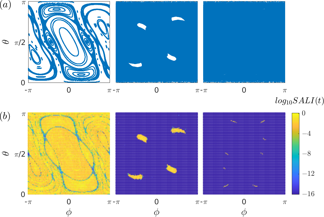
Figure 1: (a) A stroboscopic map of the classical dynamics generated from 20 random initial conditions of $5\times 10^{4}$ iterations (top panels). (b) The corresponding logarithmic values of SALI (bottom panels) on the parametrized phase space $(\theta,\phi)$ discretized by $200\times 400$ grids of square cells, of same area, after 300 kicks. The initial conditions colored dark blue correspond to chaotic orbits, the yellowish indicates ordered motion, and the intermediate suggests sticky orbits. From left to right, the kicking strength $\gamma=2,4,6$ and $\alpha=11\pi/19$.

The stroboscopic dynamics of the classical kicked top (CKT) is symplectic since $\det(\partial f/\partial\mathbf{x}_{n})=1$, and $\mathbb{S}^{2}$ as the phase space of the classical top can be parametrized as: $x=\sin\theta\cos\phi$, $y=\sin\theta\sin\phi$, $z=\cos\theta$, with $z$ and $\phi$ being the canonical pair. This map undergoes a transition from integrability to chaos with increasing kicking strength $\gamma$, as illustrated in Fig. 1(a) the Poincaré section of the classical map, for different values of $\gamma$. In the classical phase space, regular orbits predominate at small values of $\gamma$. As the kicking strength increases, mixed dynamics emerge, characterized by the coexistence of regular orbits and chaotic motion. Eventually, for larger $\gamma$, the system transitions into full chaos, as illustrated in the rightmost panel of Fig. 1(a).

To qualitatively demonstrate the transition to chaos in the classical map, in this addendum, we use the smaller alignment index (SALI) [31, 32, 33] which rely on the evolution of deviation vectors from a given orbit, to detect regular and chaotic motion of the symplectic map. For chaotic orbits, it was proved that SALI$(t)\propto e^{(-L_{1}-L_{2})t}$ [34], with $L_{1},L_{2}$ being the two largest Lyapunov exponents (LEs). While in three-dimensional symplectic map $L_{2}=0$, therefore for CKT, the SALI is directly related to the largest LE as SALI$(t)\propto e^{-L_{1}t}$. Fig. 1(b) illustrates the logarithmic SALI values after 300 kicks for grid points, at each point plotted using an assigned color according to its value. Upon comparing with the corresponding Poincaré sections in Fig. 1(a), in addition to the resemblance, we also acquire a much more detailed picture of the regions where chaotic or regular motion occurs, and at the borders between these regions we find intermediate colors which correspond to sticky orbits.

To further quantify the degree of chaos, we define the chaotic fraction $\mu_{c}$ as the relative area of the chaotic part of the phase-space as

$$\mu_{c}=\frac{1}{4\pi}\int\chi_{c}(\theta,\phi)\sin\theta d\theta d\phi,$$ (7)

where $\chi_{c}(\theta,\phi)$ denotes the characteristic function of the chaotic component, which takes the value of 1 on chaotic region and zero otherwise. The chaotic fraction $\mu_{c}$ can be used as an indicator of chaos. It measures the transition from integrable dynamics with $\mu_{c}$ = 0 to the fully chaotic (ergodic) $\mu_{c}=1$. Our criterion for the classification of initial conditions belonging to a chaotic region is that SALI$(t)\leq 10^{-8}$ at $t=300$, implying that the deviation vectors have been aligned. Calculated from $200\times 400$ initial grid points on the parametrized phase space $(\theta,\phi)$, Fig. 2(a) illustrates the dependence of the chaotic fraction $\mu_{c}$ on $\gamma$, for CKT. The value of $\mu_{c}$ remains near 0 for $\gamma\leq 2$ and increases thereafter until it saturates to 1 for $\gamma\gtrsim 4.4$. It should be noted that the transition point at $\gamma\simeq 2$ obtained by the chaotic fraction $\mu_{c}$ from the SALI method is consistent with the transition point from the Kolmogorov-Sinai entropy given in Ref. [26].

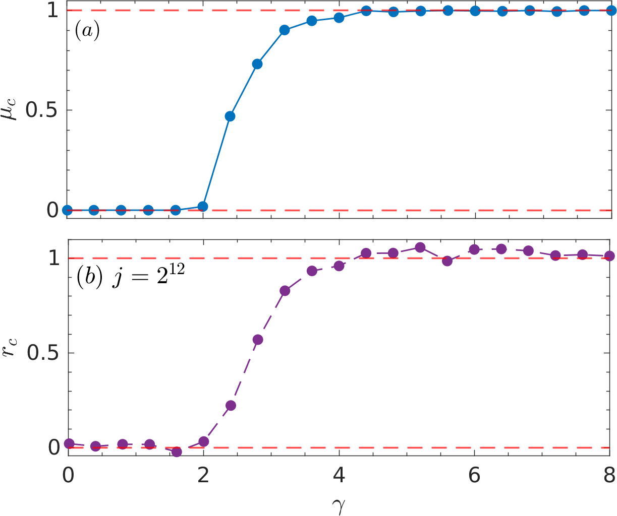
Figure 2: (a) Chaotic fraction $\mu_{c}$ of the classical phase space as a function of $\gamma$, calculated from $200\times 400$ initial grid points on the parametrized phase space $(\theta,\phi)$. (b) The normalized mean spacing ratio $r_{c}$ averaged over the odd and even parity, versus $\gamma$ for QKT with $j=2^{12}$. In both figures, the lower and upper (red) dashed lines denote the value $0$ and $1$, and the parameter $\alpha=11\pi/19$.

II.2 The transition to quantum chaos

The transition to Hamiltonian chaos, as indicated by the variation of $\mu_{c}$ versus the kicking strength in Fig. 2(a), would also be manifested in the quantum realm due to the quantum-classical correspondence. There are several methods to diagnose quantum chaos, statistically or dynamically. One is the short-range statistical properties of spectra, particularly the nearest-neighbor-level spacing distribution, denoted as $P(s)$, where $s$ denotes the spacing between two unfolded consecutive energy levels. In the quantum integrable case, this distribution follows the Poisson distribution $P(s)=e^{-s}$, whereas the quantum chaotic case with the time-reversal symmetry is the well-known Wigner-Dyson distribution $P(s)=(\pi/2)s\exp(-\pi s^{2}/4)$ from the random-matrix statistics.

To avoid the numerical spectral unfolding, we consider instead the spacing ratios, defined as [35, 36]

$$r_{n}=\min(\frac{s_{n}}{s_{n-1}},\frac{s_{n-1}}{s_{n}}),$$ (8)

with $s_{n}=\nu_{n}-\nu_{n-1}$ the consecutive level spacing, from $\{\nu_{n}\}$ an ordered set of quasienergy levels, that $F|\nu_{n}\rangle=e^{i\nu_{n}}|\nu_{n}\rangle$. The approximate formulas for the distribution of $P(r)$ can be derived from random matrix statistics. For the Poisson level spacing, the resulting mean spacing ratio $\langle r\rangle$ is $\langle r\rangle_{p}=2\ln 2-1\approx 0.386$, whereas for Circular Orthogonal Ensemble (COE) statistics, $\langle r\rangle_{COE}\approx 0.527$ [37]. We can then define a quantity $r_{c}$ the normalized mean spacing ratio as an indicator of quantum chaos, namely

$$r_{c}=\frac{\langle r\rangle-\langle r\rangle_{P}}{\langle r\rangle_{COE}-\langle r\rangle_{P}}.$$ (9)

Clearly, $r_{c}=0$ corresponds to the integrable case, while $r_{c}=1$ signifies full chaos. As discussed in Ref. [25], in QKT, there exist two antiunitary time reversal operators

$$T_{1}=e^{i\alpha J_{x}}e^{i\pi J_{z}}K,\quad T_{2}=e^{-i\alpha J_{x}}e^{i\pi J_{y}}K,$$ (10)

where $K$ denotes the conjugation in the eigenbasis of $J_{z}$. These operators satisfy $T_{1}^{2}=T_{2}^{2}=1$ and time reversal property $T_{1}FT_{1}=T_{2}FT_{2}=F^{\dagger}$. One can therefore expect that in the fully chaotic regime, the statistics of quasienergy of $F$ must be given by COE. As depicted in Fig. 2(b), the variation of $r_{c}$, averaged from both parities, with kicking strength $\gamma$ illustrates that it remains close to 0 for $\gamma\leq 2$, gradually increasing thereafter until it reaches a plateau near 1 for $\gamma\geq 4.4$. This behavior precisely aligns with the chaotic fraction $\mu_{c}$ versus $\gamma$ depicted in Fig. 2(a), as well as with the mean Wehrl entropy localization length of eigenstates, which we will demonstrate in the following.

III Husimi function and Localization of eigenstates

By employing spectral statistics, we have demonstrated in Sec. II.2 the transition to quantum chaos, which aligns with the classical route to chaos. In this section, we introduce the SCS and employ the Krylov subspace technique to numerically calculate the SCS. Notably, by avoiding the problem of large factorials, the accessible value of $j$ can be several orders of magnitude higher than those reported in the literature, including our previous work [26]. Following this, by analyzing the Husimi function of eigenstates based on SCS, we can explore the localization of these eigenstates, especially the Wehrl entropy [38] and the corresponding entropy localization measure (ELM), to a deeper semiclassical regime.

III.1 Spin coherent state and Husimi functions

The spin coherent state $|\theta,\phi\rangle$ from SU(2) [39, 40, 41], can be obtained as a rotation on the Dicke manifold, expanded in the Dicke basis $|j,m\rangle$ as

$$|\theta ,\phi\rangle=R(\theta,\phi)|j,j\rangle=\exp(\mu J_{-}-\mu^{*}J_{+})|j,j\rangle$$ (11a)

$$=(1+|\xi|^{2})^{-j}\sum_{m=-j}^{j}\binom{2j}{j+m}^{1/2}\xi^{j-m}|j,m\rangle,$$ (11b)

where $\mu=\frac{\theta}{2}\exp(i\phi)$, $\xi=\tan(\frac{\theta}{2})\exp(i\phi)$ with $\theta\in[0,\pi]$ and $\phi\in[-\pi,\pi)$, $J_{\pm}=J_{x}\pm iJ_{y}$. The SU(2) generalized coherent states $|\theta,\phi\rangle$ are overcomplete that

$$\frac{2j+1}{4\pi}\int\sin\theta d\theta d\phi\ |\theta,\phi\rangle\langle\theta,\phi|=\mathbb{I}.$$ (12)

The Husimi function of the eigenstate $|\nu_{n}\rangle$ of the Floquet operator $F$ is then given by

$$Q_{n}(\theta,\phi)=|\langle\theta,\phi|\nu_{n}\rangle|^{2},$$ (13)

with the normalization condition

$$\frac{2j+1}{4\pi}\int\sin\theta d\theta d\phi\ Q_{n}(\theta,\phi)=1.$$ (14)

Numerical studies of Husimi functions in the past usually employed Eq. (11b) for the SCS representation of quantum states. However, the presence of large factorials in this equation imposes limitations on the attainable values of $j$, typically only a few hundred. A further examination of Eq. (11a) shows that the SCS can be obtained directly from a unitary transformation of the polar state $|\theta=0,\phi\rangle=|j,j\rangle$. This unitary transformation is an exponential of a sparse matrix, because in the Dicke basis

$$J_{\pm}|j,m\rangle=\sqrt{(j\mp m)(j\pm m+1)}|j,m\pm 1\rangle.$$ (15)

Exponential of sparse matrix on vectors can be effectively computed using Krylov subspace technique (see Ref. [28]), this alternative approach bypasses the problem of large factorials and enables the attainment of significantly larger value of $j$ (differing by several orders of magnitude, depending on the sparsity), compared with the previous studies. One can take an initial look at the Husimi functions of eigenstates provided in Sec. IV.1 and more illustrations in the Appendix, where $j=2^{12}$.

III.2 Localization of eigenstates

One common way for defining the localization of eigenstates is via Shannon entropy. The eigenstates from odd parity $|\nu_{n}\rangle_{odd}$ that are expressed in the basis of unperturbed Hamiltonian, as

$$H_{n}=-\sum_{m=1}^{j}|\nu_{nm}|^{2}\ln|\nu_{nm}|^{2},\ \nu_{nk}=\langle x_{m}|\nu_{n}\rangle_{odd},$$ (16)

where $|x_{m}\rangle$ is the eigenbasis of the unperturbed Floquet part $\exp({-i\alpha J_{x}})$, i.e., the eigenbasis of $J_{x}$ in odd parity. For the even parity, it can be defined in a same way, and we have verified that the statistics of $H_{n}$ is nearly identical for both parity. This is also referred to as the eigenvector statistics. The Shannon ELM is then defined as $L_{n}=e^{H_{n}}/N_{odd}$ with $N_{odd}=j$, and the mean localization measure is denoted as $\langle L\rangle$. Apart from this basis-dependent method, another approach for measuring the localization of eigenstates is basis-independent, relying on the Wehrl entropy of eigenstates. It is defined as

$$S_{n}=-\frac{2j+1}{4\pi}\int\sin\theta d\theta d\phi\ Q_{n}(\theta,\phi)\ln Q_{n}(\theta,\phi).$$ (17)

The Wehrl ELM is $\mathcal{L}_{n}=e^{S_{n}}/N$, with $N=2j+1$ and $\langle{\mathcal{L}}\rangle$ denotes the averaging. It’s worth noting that Wehrl conjectured that the minimum of Wehrl entropy is attained for coherent state [42]. Lieb originally proved the conjecture [43], later extended it to SU(2) and SU(N) coherent states [44, 45, 46]. However, the problem of the uniqueness of minimizers in some cases is still open [47].

One may anticipate that a random eigenstate will tend to the uniform distribution that $|\nu_{nk}|^{2}=1/N_{odd}$ and $Q_{n}(\theta,\phi)=1/N$, resulting in the maximum value of both entropy $H_{n}=\ln N_{odd}$ and $S_{n}=\ln N$, as well as ELMs $L_{n}=\mathcal{L}_{n}=1$. For a random pure state $|\mathcal{R}\rangle$ from COE/GOE [48, 49], it was proved that mean Shannon entropy $\langle H\rangle_{\mathcal{R}}=\Psi(N/2+1)-\Psi(3/2)\sim\ln N+\gamma_{e}+\ln 2-2\approx\ln N-0.7296$, with $\Psi(x)$ the digamma function and $\gamma_{e}$ denotes the Euler constant, where the approximation is for the asymptotic limit $N\to\infty$. Additionally, the mean Shannon/Wehrl entropy of a random pure state from CUE is $\langle S\rangle_{\mathcal{R}}=\Psi(N+1)-\Psi(2)\sim\ln N+\gamma_{e}-1\approx\ln N-0.4228$ [50]. The random pure state statistics then gives $\langle L\rangle_{\mathcal{R}}\approx 0.482$, and $\langle\mathcal{L}\rangle_{\mathcal{R}}\approx 0.655$ for large $N$.

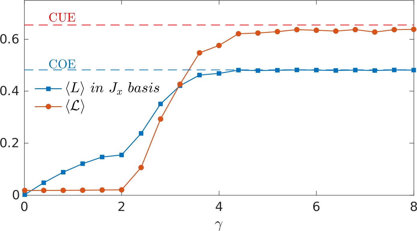
Figure 3: Mean Shannon ELM $\langle L\rangle$ from the odd parity and mean Wehrl ELM $\langle\mathcal{L}\rangle$, versus $\gamma$ for QKT with $j=2^{12}$ and $\alpha=11\pi/19$. The dashed horizontal lines indicate the mean Shannon ELM of COE and Wehrl/Shannon ELM of CUE.

In Fig. 3, we study the mean Shannon ELM $\langle L\rangle$ in the basis of $J_{x}$, for the odd parity (we found for the even parity, it is the same) and mean Wehrl ELM $\langle\mathcal{L}\rangle$. We computed the Wehrl ELM using a grid of $N_{p}=200\times 400$ points in the $(\theta,\phi)$ space, with each point holding a coherent state, where all the Husimi functions are normalized according to the discretization of Eq. (14), as

$$\frac{(2j+1)\pi}{2N_{p}}\sum_{ij}Q_{n}(\theta_{i},\phi_{j})\sin\theta_{i}=1.$$ (18)

It shows that the Shannon ELM saturates to the COE value $\langle L\rangle_{R}$ for $\gamma\gtrsim 4.4$, and before that, it exhibits two different types of growth: for $\gamma>2$, it grows faster than for $\gamma\leq 2$. While the transition versus $\gamma$ is more pronounced in the mean Wehrl ELM. For $\gamma\leq 2$, it maintains a value equal to $\langle\mathcal{L}\rangle_{J_{x}}\sim N^{-1/2}$, representing the mean Wehrl ELM of the operator $J_{x}$ (see numerical result shown in Fig. 9 and proof in Appendix A), which is close to 0 for large $N$. It then increases until it saturates for $\gamma\gtrsim 4.4$, to a value close to $\langle\mathcal{L}\rangle_{R}$ from CUE.

Numerical computations show that the mean Wehrl entropy of COE is slightly smaller than that $\langle S\rangle_{\mathcal{R}}$ from CUE, and it was conjectured in Ref. [50] that the difference vanishes in the asymptotic limit $N\to\infty$. However, both a numerical verification at larger $N$ and a formal mathematical proof for this conjecture is lacking. In Fig. 4, using the Krylov subspace technique generated coherent states, we study the mean Shannon entropy $\langle H\rangle$ and Wehrl entropy $\langle S\rangle$, of the KT at $\gamma=8$ where the system is fully chaotic. The eigenvector statistic reveals that $\langle H\rangle\simeq\ln N-0.7322$, is nearly equal to $\langle H\rangle_{\mathcal{R}}$ for COE. Similarly, for Shannon ELM, $\langle L\rangle\simeq\langle L\rangle_{\mathcal{R}}$, as shown in the inset (bottom right). On the other hand, the mean Wehrl entropy $\langle S\rangle\simeq\ln N-0.4573$, is close to $\langle S\rangle_{\mathcal{R}}$ for CUE, while the inset in the top left illustrates that $\langle\mathcal{L}\rangle$ approaches the CUE value $\langle\mathcal{L}\rangle_{\mathcal{R}}$ with increasing system size. We have examined $\langle\mathcal{L}\rangle$ against $N$ with a further increase in grid points to $N_{p}=250\times 500$, and it exhibits a similar trend.

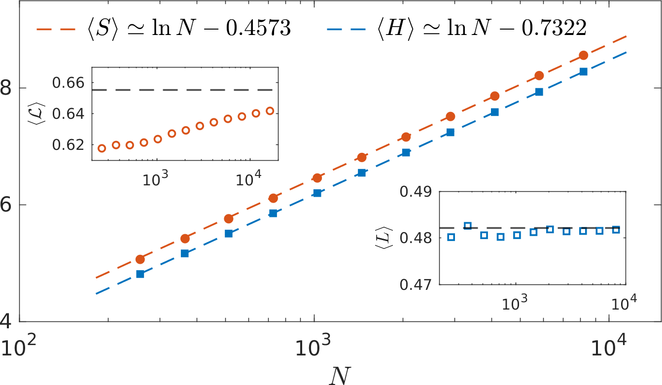
Figure 4: Mean Shannon entropy $\langle H\rangle$ and mean Wehrl entropy $\langle S\rangle$, versus $N$ for QKT, with $\gamma=8$ and $\alpha=11\pi/19$, where for the former $N=N_{odd}=j$ and the latter $N=2j+1$. Two dashed lines are from best fitting. Two insets show two mean ELMs versus $N$, respectively, where the dashed lines indicate $\langle\mathcal{L}\rangle_{\mathcal{R}}$ from CUE (top left) and $\langle L\rangle_{\mathcal{R}}$ from eigenvector statistics of COE (bottom right).

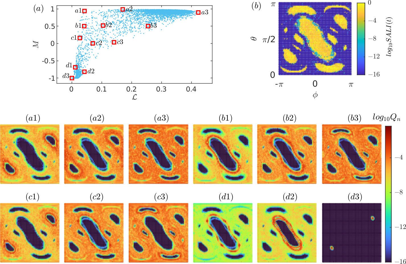
Figure 5: (a) A joint distribution $(\mathcal{L},M)$ for 8193 eigenstates of QKT Floquet operator, with $\gamma=2.6$, $\alpha=11\pi/19$ and $j=2^{12}$. Husimi functions of eigenstates isolated by boxes at different positions are plotted from panel (a1) to (d3), the darkest blues show the area where $Q_{n}<10^{-16}$. (b) Logarithmic values of SALI for the corresponding CKT, on the parametrized phase space $(\theta,\phi)$ after 300 kicks.

IV Phase-space overlap index

The Husimi functions of eigenstates in quantum maps [51, 52], are precise analog of the classical Poincaré section. From this correspondence, the Husimi functions of eigenstates can be used for the identification of regular, mixed, and chaotic eigenstates, by the criterion of overlap with the classical Poincaré section, where one can employ the SALI method to identify whether an initial condition belongs to the classical chaotic or regular regions. As it was introduced and implemented in previous works [53, 54, 55], for eigenstate $|\nu_{n}\rangle$, the overlap can be quantified by the overlap index $M_{n}$, defined as

$$M_{n}=\frac{2j+1}{4\pi}\int\sin\theta d\theta d\phi\ f(\chi_{c})Q_{n}(\theta,\phi),$$ (19)

where $f(\chi_{c})=1$ if $\chi_{c}=1$, and $f(\chi_{c})=-1$ if $\chi_{c}=0$. Here, $\chi_{c}(\theta,\phi)$ denotes the characteristic function of the chaotic component, as defined in Eq. (7).

According to PUSC in mixed-type systems, for Husimi functions of eigenstates, $M$ should be either $+1$ or $-1$ in the strict semiclassical limit, corresponding to chaotic or regular eigenstates, respectively. However, since the semiclassical limit is not easily reached in practice, $M$ actually varies between $-1$ and $+1$. Upon approaching the semiclassical limit, a reduction in the fraction of mixed eigenstates with $|M|<1$ would occur, as evidenced first in the billiard system [23], particularly exhibiting a power-law decay with increasing energy, i.e. decreasing effective Planck constant. In the following, we analyze quantum eigenstates of Floquet operator in mixed-type QKT by studying the joint distribution of Wehrl ELM and overlap index. Then, we extend the analysis of the power-law decay of the fraction of mixed eigenstates as system size increases, as conducted in Ref. [26], up to $j=2^{13}$. For numerical calculation of Husimi functions, we use a grid of $N_{p}=200\times 400$ points in the $(\theta,\phi)$ space, with each point holding a coherent state.

IV.1 The overlap index and Wehrl ELM

From the definition of Wehrl ELM following Eq. (17), regular eigenstates characterized by an overlap index of $M=-1$ and condensing on invariant tori are localized, yielding lower values of $\mathcal{L}$. In contrast, chaotic eigenstates with $M=+1$ can be either strongly localized or extended. Previous studies have numerically shown that the probability distribution $P(\mathcal{L})$ of chaotic eigenstates indeed follows a beta distribution [56, 57, 58]. As the system approaches the semiclassical limit, it tends towards a delta distribution $\delta(\mathcal{L}-\langle\mathcal{L}\rangle_{\mathcal{R}})$. It is important to note that in mixed-type systems, to verify this distribution, the Wehrl ELM of the chaotic eigenstates should be further renormalized by the relative area $\mu_{c}$ of the chaotic component in the phase space. In addition to strictly regular and chaotic states, there would exist mixed eigenstates with $|M|<1$ in mixed-type systems, exhibiting varying degrees of localization. This is illustrated in Fig. 5(a) the joint distribution $(\mathcal{L},M)$ for KT at $\gamma=2.6$, alongside selected representative Husimi functions of eigenstates from different regions of the parameter space, as shown in Fig. 5(a1)-(d3). Moreover, Fig. 5(b) presents the SALI plot from the corresponding classical dynamics at $\gamma=2.6$ in phase space, for comparison. At the border of the regular islands and chaotic sea, visible stickiness are denoted by intermediate colors.

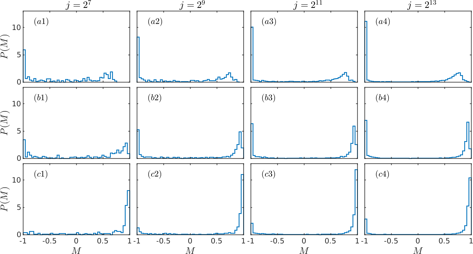
Figure 6: Histograms of $P(M)$ for increasing system size, from left to right. In panels (a1)-(a4), the kicking strength is set to $\gamma=2.3$. In panels (b1)-(b4), it is $\gamma=2.6$, and in panels (c1)-(c4), it is $\gamma=3$.

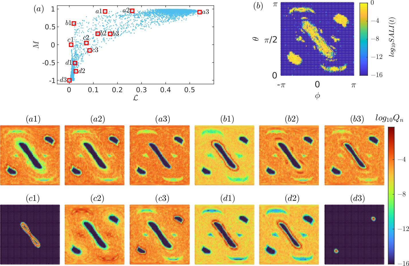
Figure 11: Analogous data as in Fig. 5 and 10, but now for $\gamma=3$. Compared with $\gamma=2.3$, in this case, the fixed point at $(\theta,\phi)=(\pi/2,0)$ becomes unstable, which is clearly shown in the SALI plot. Interestingly, the most localized state (d3) occupies identical fixed points, akin to when $\gamma=2.6$.

Fig. 5 shows that states predominantly cluster at both ends of the overlap index, one end representing regular states and the other chaotic states, while mixed states sparsely distribute in between. This clustering is more evident for QKT at $\gamma=3$, as shown in Fig. 11 (see Appendix B the gallery of states), where larger values of $\gamma$ correspond to increased $\mu_{c}$ the fraction of chaotic components, and a simpler structure of classical phase space. Examining Husimi functions of the chaotic eigenstates plotted in Fig. 5(a1)-(a3), alongside the corresponding SALI plot, a reduction in the area of the darkest blue regions (with $Q_{n}\leq 10^{-16}$) belonging to regular islands can be observed. The most extended state shown in Fig. 5(a3), infiltrates into the regular islands due to quantum tunneling, and exhibits a minor overlap with the outer tori of the regular islands. The state with the maximum overlap index, as plotted in Fig. 5(a1), is strongly localized around and avoids the outer tori of the regular region. Similar observation extends to another layer of overlap index $M\simeq 0.5$ for states illustrated in Fig. 5(b1)-(b3), and to $M\simeq 0$ in Fig. 5(c1)-(c3), except that the most localized ones now live in the vicinity of the regular islands, with smaller contribution from the chaotic sea. Fig. 5(d1)-(d3) illustrate states from the bottom layer of overlap index. Particularly, Fig. 5(d1) shows a state predominantly localized at a chain of regular islands, which exhibits tunneling between these regular islands. In Fig. 5(d2), the state also resides in the vicinity of the regular island, with visible stickiness surrounding it, appearing more extended. The most localized state shown in Fig. 5(d3) is located exactly at the fixed points.

In summary, the joint distribution $(\mathcal{L},M)$ offers a comprehensive overview of mixed-type QKT eigenstates. The study of Husimi functions shows that, mixed states predominantly occupy chaotic regions with $M>0$, flooding into regular areas, while states concentrate in regular islands with $M<0$, displaying tunneling between them. Furthermore, among states with a smaller overlap index, the Wehrl ELM shows a narrower range.

IV.2 The fraction of mixed eigenstates

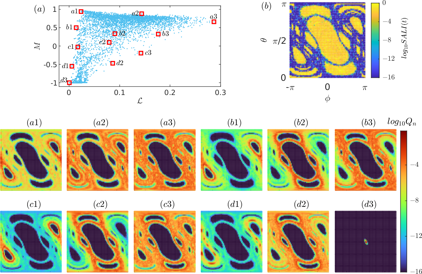
Figure 10: Analogous data as in Fig. 5, but for $\gamma=2.3$. The darkest blues in the plots of Husimi functions from (a1)-(d3) show the area where $Q_{n}<10^{-16}$. The most localized state (d3) precisely located at the (trivial) fixed point $(\theta,\phi)=(\pi/2,0)$, while the state (a1) of the maximum overlap index, is strongly localized around and avoids the outer tori of the regular region.

In the semiclassical limit, it is expected that mixed states gradually disappear in accordance with the Berry-Robnik picture and PUSC. This is supported by the histograms depicted in Fig. 6, which illustrate the distribution $P(M)$ of the overlap index $M$ as the system size $j$ increases, at different kicking strengths. As the semiclassical limit is approached with increasing $j$, we observe that: (i) Increasing values of $j$ lead to a more pronounced alignment of eigenstates with either regular or chaotic clusters. Specifically, at $\gamma=2.3$, the kicking strength closer to the integrability breaking at $\gamma\simeq 2$, the chaotic cluster centers around $M\simeq 0.8$, correlating with a much more complex phase space structure (see Fig. 10 in Appendix B) and the possible classical partial transport barriers [59, 60, 61, 62, 63, 64]. (ii) Fluctuations among intermediate values of $M$ decrease as the system size $j$ increases. (iii) Increasing $\gamma$ enhances chaos and $\mu_{c}$, reflected in $P(M)$ with a higher peak at $M=+1$ and a lower peak at $M=-1$, and reduced fluctuations for $|M|<1$.

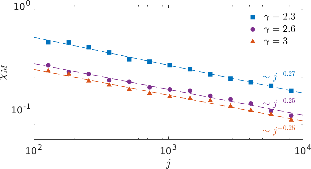
Figure 7: Decay of the fraction of mixed eigenstates $\chi_{M}$ with respect to $j$, at three kicking strengths $\gamma=2.3$ (squares), $\gamma=2.6$ (circles) and $\gamma=3$ (triangles). The mixed eigenstates criteria here is $M\in[-0.9,0.5]$. The dashed lines show the power law decay of $\chi_{M}\sim j^{-\zeta}$.

Following these observations, to quantify the decay of the fraction of mixed states with respect to the increasing system size $j$, we define

$$\chi_{M}=N(M\in[M_{0},M_{1}])/N,$$ (20)

as the fraction of eigenstates within an interval of the overlap index $M_{0}\leq M\leq M_{1}$, given the total number of states $N=2j+1$. In Fig. 7, we show the case where $M\in[-0.9,0.5]$ and plot $\chi_{M}$ as a function of $j$ for different $\gamma$. This behavior is well described (fitted) by a power-law decay, $\chi_{M}\sim j^{-\zeta}$, with the power exponent $\zeta$ being very similar for different $\gamma$. Here, the range of $j$ we considered is expanded by two orders of magnitude compared to the previous study [26], which only examined $j$ up to 400, resulting in substantially improved fitting.

The decay exponent $\zeta$ certainly depends on the interval we consider for $M$. The interval should not be too small, lacking sufficient states for good statistics, or too large to show little variation across different intervals. In Fig. 8, we illustrate the variation of the decay exponent when considering small intervals $M\in[M-\Delta M/2,M+\Delta M/2]$, with $\Delta M=0.3$, for different $\gamma$. The inset displays the goodness of the best-fitting, indicated by $R^{2}$, the coefficient of determination. Disregarding a few imperfect fittings, the data suggests a decay exponent range of $0.2<\zeta<0.45$. Given the similar power-law decay observed in the fraction of mixed eigenstates in both billiards [23] and quantum Henon-Heilés system [58], along with the Dicke model [65], we conjecture that this behavior is a universal property of mixed states, as the system approaches the semiclassical limit. A more profound open question is whether there exists an upper bound of the decay exponent.

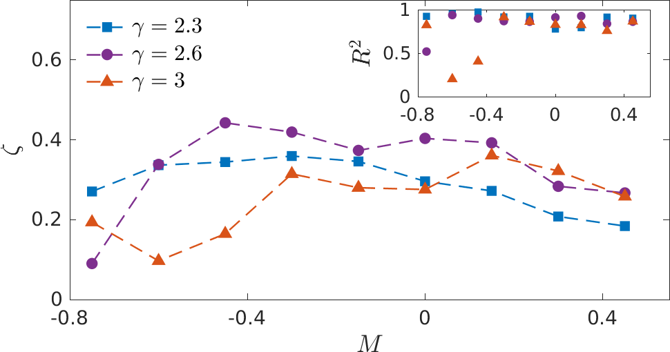
Figure 8: Power-law decay exponent $\zeta$ for $M\in[M-\Delta M/2,M+\Delta M/2]$, with $\Delta M=0.3$, across different intervals. The inset shows the goodness of all best-fittings, indicated by the coefficient of determination $R^{2}$.

We emphasize that in Ref. [22], the hierarchical states were introduced as a new class of eigenstates in mixed-type systems, distinct from the regular and chaotic ones. These states, observed in the quantum kicked rotor with much simpler phase space structure, predominantly live near the regular islands, with only a minor contribution in the main part of the chaotic sea. They also demonstrate a power-law decay $\hbar^{\alpha}\ (\alpha>0)$, attributed to the transport properties associated with stickiness between regular islands and the chaotic sea. From this definition, the hierarchical states mostly are highly localized states as shown in Fig. 5(b1), (c1), (d1) (or the same labeled states in Fig. 10-11). While the overlap index captures all the mixed states across different degrees of localization, it is influenced also by the flooding of chaotic sea to regular islands or the tunneling between regular islands, not directly related to the effects of classical stickiness. So it would be interesting to study the behavior of mixed states in systems without classical stickiness, like certain lemon billiards [66, 67].

V Conclusions

In this work, we employed the Krylov subspace technique to generate spin coherent states, thereby extending the investigation of the statistics of Husimi functions of eigenstates in the kicked top, a prototype model for studying quantum chaos. Notably, we explored system sizes up to $j=2^{13}$, a significant advancement compared to previous studies of Husimi functions limited to $j$ in the range of a few hundred. We examined the transition to chaos in both classical and quantum case. All the indicators show a good quantum-classical correspondence, specifically the mean Wehrl entropy localization measure in the statistics of eigenstates. With this new spin coherent states generating method, we also demonstrated that the mean Wehrl entropy localization measure of the fully chaotic quantum kicked top, which follows the COE spectral statistics, approaches the CUE value as the system size $j$ increases, which is surprising [50].

More importantly, in the case of a mixed-type kicked top where regular islands and chaotic sea coexist in the classical compact phase space, we examined mixed eigenstates using a joint distribution of the overlap index $M$ and Wehrl localization measure $\mathcal{L}$. $M=+1$ indicates chaotic states, while $M=-1$ indicates regular ones. We extended the study of mixed eigenstates with $|M|<1$ in our previous investigation [26] from $j=400$ to $j=2^{13}$, confirming the power-law decay of the fraction of mixed states across two orders of magnitude in $j$. This provides supporting evidence for the PUSC and the Berry-Robnik picture in the semiclassical limit. Based on this result from quantum kicked top, and similar results from other models [23, 58, 65], we conjecture that the power-law decay is a universal property for mixed eigenstates. This hypothesis merits further theoretical scrutiny.

VI Acknowledgement

This work was supported by the Slovenian Research and Innovation Agency (ARIS) under the grant J1-4387.

Appendix A Mean ELM in integrable QKT

In Fig. 3 we have shown that the mean Wehrl ELM $\langle\mathcal{L}\rangle$ of KT maintains a value equal to the mean Wehrl ELM of the unperturbed Hamiltonian $\langle\mathcal{L}\rangle_{J_{x}}$, for $\gamma\leq 2$, which is almost integrable. Fig. 9 shows that at $\gamma=1$, the mean Wehrl entropy $\langle S\rangle\sim\frac{1}{2}\ln N$ and accordingly in the inset $\langle\mathcal{L}\rangle\sim N^{-1/2}$. When contrasting with the uniformly chaotic systems where $\langle S\rangle\sim\ln N$ and $\langle\mathcal{L}\rangle\sim 1$, the distinction between integrable and chaotic cases becomes apparent (see Fig. 4 for the behavior of $\langle S\rangle$ and $\langle\mathcal{L}\rangle$ at $\gamma=8$). In integrable regimes, eigenstates tend to cover a thin band around a circle on the sphere, whereas in chaotic regimes, eigenstates exhibit delocalization across the entire sphere [24].

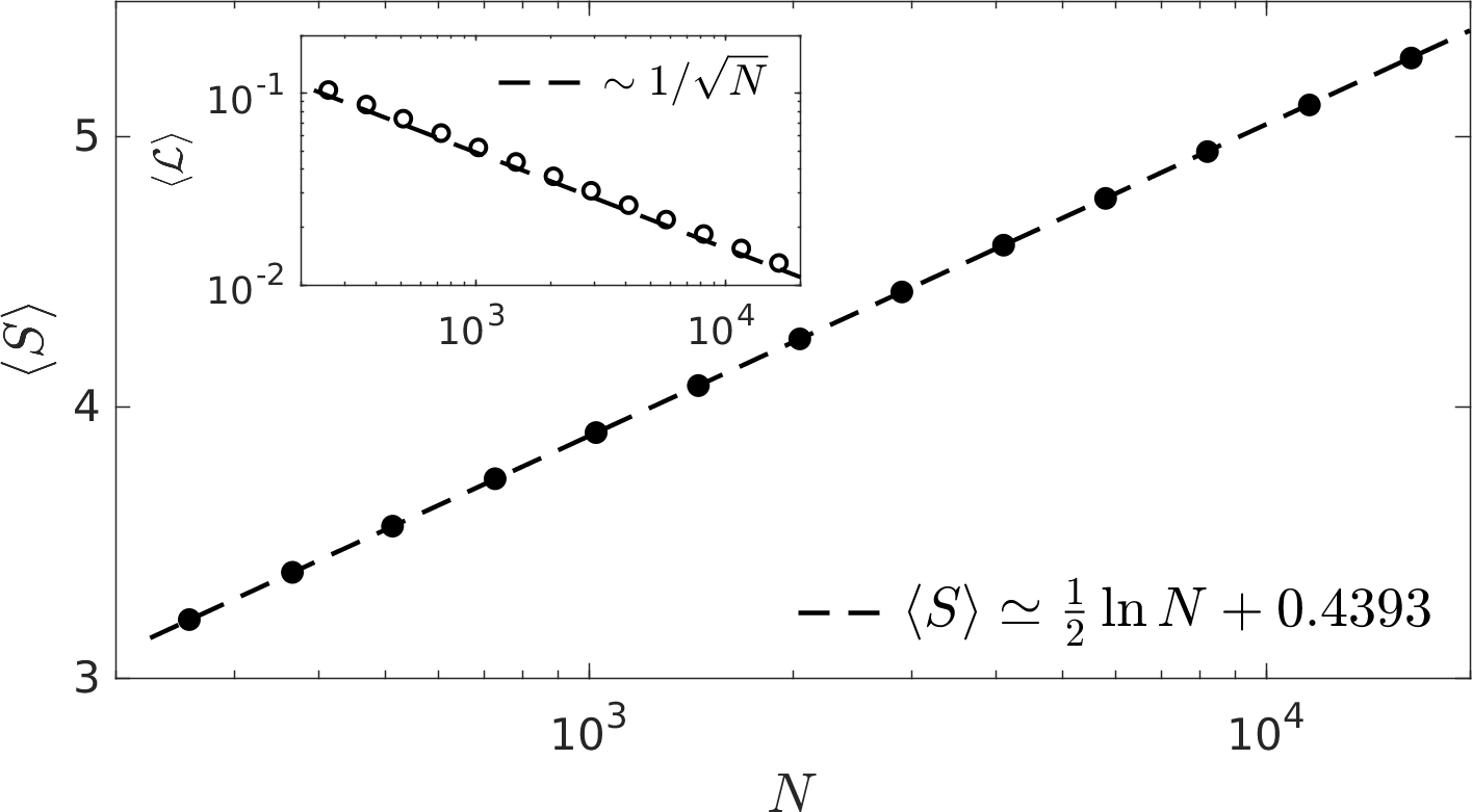
Figure 9: Mean Wehrl entropy $\langle S\rangle$, versus $N=2j+1$ for QKT with $\gamma=1$ and $\alpha=11\pi/19$. The inset is for mean Wehrl ELM $\langle\mathcal{L}\rangle$. The dashed lines indicate the best fittings.

To derive the scaling of the mean Wehrl entropy of $J_{x}$, it is first necessary to prove that $\langle S\rangle_{J_{x}}=\langle S\rangle_{J_{z}}$. While eigenvectors $|j,m\rangle_{x}$ of $J_{x}$ is a unitary transformation of eigenvectors of $J_{z}$, i.e. the Dicke basis $|j,m\rangle$, as

$$|j,m\rangle_{x} =\exp(-i\pi J_{y}/2)|j,m\rangle$$

$$=R(-\pi/2,0)|j,m\rangle=\sum_{m^{\prime}}d_{m^{\prime}m}^{j}(\pi/2)|m^{\prime}\rangle,$$ (21)

where $R(\theta,\phi)$ is given in Eq. (11a), $d_{mm^{\prime}}^{j}(\theta)$ is the Wigner $d$-matrix. Moreover, $R(\pi,0)|j,m\rangle=|j,-m\rangle$ while $R(\pi,0)K$ is the conventional time-reversal operator and $K$ is the complex conjugation on Dicke basis. The summation of the mean $q$-moment of Husimi functions of all the eigenvectors of $J_{x}$ can then be written as

$$\frac{1}{N}\sum_{m}W_{|m\rangle_{x}}^{(q)}=\frac{1}{4\pi}\sum_{m}\int d\Omega|\langle\theta,\phi|j,m\rangle_{x}|^{2q}$$

$$=\frac{1}{4\pi}\sum_{m}\int d\Omega\left|\langle j,j|R^{\dagger}(\theta,\phi)R(-\frac{\pi}{2},0)|j,m\rangle\right|^{2q},$$ (22)

where $d\Omega=\sin\theta d\theta d\phi$, and $N=2j+1$. Following Eq. (11b), we can further expand Eq. (A) with the properties of the Wigner $d$-matrix: $d_{mm^{\prime}}^{j}(\theta)=d_{m^{\prime}m}^{j}(-\theta)=(-1)^{m^{\prime}-m}d_{m^{\prime}m}^{j}(\theta)$, for integer $q$. It yields

$$\frac{1}{4\pi}\sum_{m}\int d\Omega\big{|}(1+|\xi|^{2})^{-j}\sum_{m^{\prime}}\binom{2j}{j+m^{\prime}}^{\frac{1}{2}}\xi^{j-m^{\prime}}d_{m^{\prime}m}^{j}(\frac{\pi}{2})\big{|}^{2q}$$

$$=\frac{1}{4\pi}\sum_{m}\int d\Omega\big{|}(1+|\xi|^{2})^{-j}\sum_{m^{\prime}}\binom{2j}{j+m^{\prime}}^{\frac{1}{2}}\xi^{j-m^{\prime}}\big{|}^{2q}$$

$$=\frac{1}{4\pi}\sum_{m}\int d\Omega|\langle\theta,\phi|j,m\rangle|^{2q}=\frac{1}{N}\sum_{m}W_{|m\rangle}^{(q)}.$$ (23)

Considering the equivalence of mean $q$-moments, we establish that $\langle S\rangle_{J_{x}}=\langle S\rangle_{J_{z}}$, as $S^{(q)}_{|\psi\rangle}=\frac{1}{1-q}\ln W^{(q)}_{|\psi\rangle}$. While for Dicke states, it was proved that [68]

$$S_{|m\rangle}=\frac{2j}{2j+1}-\ln\binom{2j}{j-m}+2j\Psi(2j+1)$$

$$-(j+m)\Psi(j+m+1)-(j-m)\Psi(j-m+1),$$ (24)

where $\Psi(x)$ denotes the digamma function, and obviously $S_{|m\rangle}=S_{|-m\rangle}$. Therefore,

$$\langle S\rangle_{J_{z}}=\frac{1}{N}\sum_{m=-j}^{j}S_{|m\rangle}=\frac{2j}{2j+1}-\ln(2j)!+2jB_{2j}$$

$$+\frac{2}{2j+1}\sum_{m}\left[\ln(j+m)!-(j+m)B_{j+m}\right],$$ (25)

where $B_{n}=\sum_{k=1}^{n}\frac{1}{k}\approx\ln n+\gamma_{e}$. Applying Stirling’s approximation to factorials $\ln n!\approx n\ln n+\frac{1}{2}n-n$, for $j\to\infty$, one then gets $\langle S\rangle_{J_{z}}\sim\frac{1}{2}\ln N$. Consequently, the mean ELM $\langle\mathcal{L}\rangle$ scales as $N^{-1/2}$, the same scaling as the width of effective Planck cell $j^{-1/2}\propto N^{-1/2}$.

Appendix B Gallery of states

Here, we provide additional examples of the joint distribution $(\mathcal{L},M)$ for mixed-type QKT, along with representative Husimi functions of eigenstates from different regions of the parameter space, at two kicking strengths $\gamma=2.3$ and $3$, accompanied by corresponding SALI plots.

References

- Percival [1973] I. Percival, Journal of Physics B: Atomic and Molecular Physics 6, L229 (1973).
- Berry [1977] M. V. Berry, Journal of Physics A: Mathematical and General 10, 2083 (1977).
- Lichtenberg and Lieberman [2013] A. J. Lichtenberg and M. A. Lieberman, Regular and chaotic dynamics, Vol. 38 (Springer Science & Business Media, 2013).
- Robnik [1998] M. Robnik, Nonlinear Phenomena in Complex Systems 1, 1 (1998).
- Srednicki [1994] M. Srednicki, Physical Review E 50, 888 (1994).
- Rigol et al. [2008] M. Rigol, V. Dunjko, and M. Olshanii, Nature 452, 854 (2008).
- D’Alessio et al. [2016] L. D’Alessio, Y. Kafri, A. Polkovnikov, and M. Rigol, Advances in Physics 65, 239 (2016).
- Wang et al. [2022] J. Wang, M. H. Lamann, J. Richter, R. Steinigeweg, A. Dymarsky, and J. Gemmer, Physical Review Letters 128, 180601 (2022).
- Berry and Tabor [1977] M. V. Berry and M. Tabor, Proceedings of the Royal Society of London. A. Mathematical and Physical Sciences 356, 375 (1977).
- Casati et al. [1980] G. Casati, F. Valz-Gris, and I. Guarnieri, Lettere al Nuovo Cimento (1971-1985) 28, 279 (1980).
- Bohigas et al. [1984] O. Bohigas, M.-J. Giannoni, and C. Schmit, Physical review letters 52, 1 (1984).
- Müller et al. [2004] S. Müller, S. Heusler, P. Braun, F. Haake, and A. Altland, Physical review letters 93, 014103 (2004).
- Berry and Robnik [1984] M. V. Berry and M. Robnik, Journal of Physics A: Mathematical and General 17, 2413 (1984).
- Tomsovic and Ullmo [1994] S. Tomsovic and D. Ullmo, Physical Review E 50, 145 (1994).
- Bohigas et al. [1993] O. Bohigas, S. Tomsovic, and D. Ullmo, Physics Reports 223, 43 (1993).
- Doron and Frischat [1995] E. Doron and S. D. Frischat, Physical review letters 75, 3661 (1995).
- Bäcker et al. [2005] A. Bäcker, R. Ketzmerick, and A. G. Monastra, Physical review letters 94, 054102 (2005).
- Brodier et al. [2001] O. Brodier, P. Schlagheck, and D. Ullmo, Physical Review Letters 87, 064101 (2001).
- Bäcker et al. [2008a] A. Bäcker, R. Ketzmerick, S. Löck, and L. Schilling, Physical review letters 100, 104101 (2008a).
- Bäcker et al. [2008b] A. Bäcker, R. Ketzmerick, S. Löck, M. Robnik, G. Vidmar, R. Höhmann, U. Kuhl, and H.-J. Stöckmann, Physical review letters 100, 174103 (2008b).
- Löck et al. [2010] S. Löck, A. Bäcker, R. Ketzmerick, and P. Schlagheck, Physical review letters 104, 114101 (2010).
- Ketzmerick et al. [2000] R. Ketzmerick, L. Hufnagel, F. Steinbach, and M. Weiss, Physical Review Letters 85, 1214 (2000).
- Lozej et al. [2022] Č. Lozej, D. Lukman, and M. Robnik, Physical Review E 106, 054203 (2022).
- Haake [2013] F. Haake, Quantum Signatures of Chaos, Vol. 54 (Springer Science & Business Media, 2013).
- Haake et al. [1987] F. Haake, M. Kuś, and R. Scharf, Zeitschrift für Physik B Condensed Matter 65, 381 (1987).
- Wang and Robnik [2023] Q. Wang and M. Robnik, Physical Review E 108, 054217 (2023).
- Sidje [1998] R. B. Sidje, ACM Transactions on Mathematical Software (TOMS) 24, 130 (1998).
- Moler and Van Loan [2003] C. Moler and C. Van Loan, SIAM review 45, 3 (2003).
- Golub and Van Loan [2013] G. H. Golub and C. F. Van Loan, Matrix computations (JHU press, 2013).
- Saad [2003] Y. Saad, Iterative methods for sparse linear systems (SIAM, 2003).
- Skokos [2001] C. Skokos, Journal of Physics A: Mathematical and General 34, 10029 (2001).
- Skokos et al. [2003] C. Skokos, C. Antonopoulos, T. C. Bountis, and M. N. Vrahatis, Progress of Theoretical Physics Supplement 150, 439 (2003).
- Skokos et al. [2004] C. Skokos, C. Antonopoulos, T. Bountis, and M. Vrahatis, Journal of Physics A: Mathematical and General 37, 6269 (2004).
- Bountis and Skokos [2012] T. Bountis and H. Skokos, Complex hamiltonian dynamics, Vol. 10 (Springer Science & Business Media, 2012).
- Oganesyan and Huse [2007] V. Oganesyan and D. A. Huse, Physical Review B 75, 155111 (2007).
- Atas et al. [2013] Y. Atas, E. Bogomolny, O. Giraud, and G. Roux, Physical review letters 110, 084101 (2013).
- D’Alessio and Rigol [2014] L. D’Alessio and M. Rigol, Physical Review X 4, 041048 (2014).
- Wehrl [1978] A. Wehrl, Reviews of Modern Physics 50, 221 (1978).
- Perelomov [1972] A. M. Perelomov, Communications in Mathematical Physics 26, 222 (1972).
- Klauder and Skagerstam [1985] J. R. Klauder and B.-S. Skagerstam, Coherent states: applications in physics and mathematical physics (World scientific, 1985).
- Zhang et al. [1990] W.-M. Zhang, R. Gilmore, et al., Reviews of Modern Physics 62, 867 (1990).
- Wehrl [1979] A. Wehrl, Reports on Mathematical Physics 16, 353 (1979).
- Lieb [1978] E. H. Lieb, Communications in Mathematical Physics 62, 35 (1978).
- Lieb and Solovej [1991] E. H. Lieb and J. P. Solovej, letters in mathematical physics 22, 145 (1991).
- Lieb and Solovej [2014] E. H. Lieb and J. P. Solovej, Acta Mathematica 212, 379 (2014).
- Lieb and Solovej [2016] E. H. Lieb and J. P. Solovej, Communications in Mathematical Physics 348, 567 (2016).
- Schupp [2022] P. Schupp, arXiv preprint arXiv:2203.08095 (2022).
- Wootters [1990] W. K. Wootters, Foundations of Physics 20, 1365 (1990).
- Jones [1990] K. R. Jones, Journal of Physics A: Mathematical and General 23, L1247 (1990).
- Gnutzmann and Zyczkowski [2001] S. Gnutzmann and K. Zyczkowski, Journal of Physics A: Mathematical and General 34, 10123 (2001).
- Bogomolny [1992] E. B. Bogomolny, Nonlinearity 5, 805 (1992).
- Prosen [1996] T. Prosen, Physica D: Nonlinear Phenomena 91, 244 (1996).
- Batistić and Robnik [2013a] B. Batistić and M. Robnik, Journal of Physics A: Mathematical and Theoretical 46, 315102 (2013a).
- Batistić et al. [2013] B. Batistić, T. Manos, and M. Robnik, Europhysics Letters 102, 50008 (2013).
- Batistić and Robnik [2013b] B. Batistić and M. Robnik, Physical Review E 88, 052913 (2013b).
- Batistić et al. [2019] B. Batistić, Č. Lozej, and M. Robnik, Physical Review E 100, 062208 (2019).
- Batistić et al. [2020] B. Batistić, Č. Lozej, and M. Robnik, Nonlinear Phenomena in Complex Systems 23, 17 (2020).
- Yan and Robnik [2024] H. Yan and M. Robnik, arXiv preprint arXiv:2401.13070 (2024).
- MacKay et al. [1984] R. MacKay, J. Meiss, and I. Percival, Physica D: Nonlinear Phenomena 13, 55 (1984).
- Geisel et al. [1986] T. Geisel, G. Radons, and J. Rubner, Physical review letters 57, 2883 (1986).
- Bohigas et al. [1990] O. Bohigas, S. Tomsovic, and D. Ullmo, Physical review letters 64, 1479 (1990).
- Michler et al. [2012] M. Michler, A. Bäcker, R. Ketzmerick, H.-J. Stöckmann, and S. Tomsovic, Physical Review Letters 109, 234101 (2012).
- Stöber et al. [2024] J. Stöber, A. Bäcker, and R. Ketzmerick, Physical Review Letters 132, 047201 (2024).
- Meiss [2015] J. Meiss, Chaos: An Interdisciplinary Journal of Nonlinear Science 25 (2015).
- Wang and Robnik [2024] Q. Wang and M. Robnik, Physical Review E 109, 024225 (2024).
- Lozej et al. [2021a] C. Lozej, D. Lukman, and M. Robnik, Nonlinear Phenomena in Complex Systems 24, 1 (2021a).
- Lozej et al. [2021b] Č. Lozej, D. Lukman, and M. Robnik, Physical Review E 103, 012204 (2021b).
- Lee [1988] C. T. Lee, Journal of Physics A: Mathematical and General 21, 3749 (1988).