Effects of gravitational waves on electromagnetic fields
Abstract
We focus on the interaction of a plane gravitational wave with electromagnetic fields and we describe this interaction in the proper detector frame where, thanks to the introduction of Fermi coordinates, it is possible to refer to directly measurable quantities. The presence of a gravitational field can be addressed in terms of an effective electromagnetic medium and, within this framework, we show that the coupling of pre-existing electromagnetic fields with the gravitational field of the wave gives rise to new effective currents. To assess the impact of these effects, we solve Maxwell’s equations for some standard configurations of the electric and magnetic fields.
I Introduction
After their first direct interferometric detection Abbott et al. (2016), gravitational waves have opened a new window for research in astrophysics and cosmology: in fact, gravitational waves are important not only because they constitute yet another test of Einstein’s theory Will (2015), but also because they serve as crucial instruments for exploring the universe in the age of multi-messenger astronomy. Advancements in technology and specialized missions are poised to significantly enhance the wealth of information accessible through this avenue (for further details, see, e.g., Miller and Yunes (2019); Bailes et al. (2021) and related references).
Furthermore, experiments with gravitational waves are crucial for testing gravitational theories beyond General Relativity. Indeed, challenges to Einstein’s theory emerge from observations of the universe on a large scale, with the problems of dark matter and dark energy Debono and Smoot (2016), and at a more fundamental level we still don’t know how to reconcile General Relativity with the Standard Model of particle physics. In order to try to cope with these issues, theories with additional fields (such as scalar ones) or provided with a richer geometrical structure were proposed and, in these cases, gravitational waves might have different features with respect to the general relativistic ones, such as for instance longitudinal effects (see e.g. Capozziello and de Laurentis (2011)). These motivations drive enormous efforts to further develop current interferometers, such as LIGO and VIRGO, as well as to design and create brand new ones, such as LISA.
More generally, investigations on gravitational waves do not solely rely on interferometers, where changes in relative distances between test masses are measured using lasers. Other Earth-based experimental setups have been proposed, including accelerators Rao et al. (2020, 2023), storage rings Berlin et al. (2021), two-level system resonance Ruggiero and Ortolan (2020a) and microcavities Berlin et al. (2022). In the latter case, particularly, researchers study the effects of gravitational waves on electromagnetic fields in resonant cavity experiments. So, the interaction between gravitational waves and electromagnetic fields, which has extensively been studied (see e.g. Cooperstock and Faraoni (1993); Fortini et al. (1996); Montanari (1998); Mieling et al. (2021) and references therein) presents potential for exploring new experimental paths.
The purpose of this paper is to develop a formalism to study the effect of a plane gravitational wave on electromagnetic fields. In order to do this, we solve Maxwell’s equation in the curved spacetime of a plane gravitational wave and we do this in the proper detector frame. Indeed, gravitational waves are typically studied using the transverse and traceless (TT) tensor, which allows to introduce the so-called TT coordinates or TT frame. The proper detector frame is an alternative approach Maggiore (2007) which is based on the use of Fermi coordinates. The latter are a quasi-Cartesian coordinates system that can be build in the neighbourhood of the world-line of an observer, and their definition depends both on the background field where the observer is moving and, also, on the kind of motion. Fermi coordinates are defined, by construction, as scalar invariants Synge (1960); they have a concrete meaning, since they are the coordinates an observer would naturally use to make space and time measurements in the vicinity of his/her world-line.
Recently, the interaction of gravitational waves and electromagnetic fields has been studied in the TT frame by Cabral and Lobo (2017); here we use the alternative approach described above and, in addition, we use a formalism that allows Maxwell’s equations in curved spacetime to be written as flat spacetime equations in the presence of an anisotropic medium. Subsequently, some simplified interaction models will be discussed to understand and evaluate the impact of a plane gravitational wave on the electromagnetic fields already present before its passage.
The paper is organized as follows: in Section II we introduce the formalism to study Maxwell’s equations in curved spacetime, while in Section III we focus on the construction of the local spacetime metric in the laboratory frame, with the use of Fermi coordinates, and we apply it to the field of a plane gravitational wave. Next, in Section IV, we present the fundamental equations necessary for investigating the influence of gravitational waves on electromagnetic fields, followed by their solution in select prototypical scenarios. Subsequently, discussion and conclusions are provided in Section VI.
II Maxwell’s equations in curved spacetime
We aim to investigate the influence of gravitational waves on electromagnetic fields. To achieve this, we must solve Maxwell’s equations in curved spacetime. If is the antisymmetric tensor of the electromagnetic field, the equations that determine the electromagnetic field in curved spacetime are111Latin indices refer to space coordinates, while Greek indices to spacetime ones. We will use bold-face symbols like to refer to space vectors; the spacetime signature is in our convention. Landau and Lifshitz (2013); Misner et al. (1973):
| (1) | |||||
| (2) |
where “;” indicates covariant derivative, and is the four-current. The above equations, due to the antisymmetry of the electromagnetic tensor, can be also written in the form
| (3) | |||||
| (4) |
where “,” stands for partial derivative, and is the determinant of the spacetime metric. The covariant electromagnetic tensor is usually defined in terms of the three-dimensional electric and magnetic fields222We use Cartesian coordinates here and henceforth. and
| (5) |
The above equations (3)-(4) can be simplified and written like Maxwell’s equations in flat spacetime in a medium (see e.g. Plebanski (1960); Mashhoon (1973); Leonhardt and Philbin (2006, 2009) and references therein). To do this, we introduce such that
| (6) |
which contains the fields and since
| (7) |
Now, if we set
| (8) |
the source equations (4) can be written in the form
| (9) |
In other words, Maxwell’s source equations in curved spacetime are written in the form of electromagnetic equations in flat spacetime in a material medium, with current , with the constitutive equations given by (6). The homogenous equations (3) are instead expressed in terms of the fields as in flat spacetime. In three dimensional notation we have
| (10) |
Using Eq. (6), it is possible to obtain the relation between . In fact, we get
| (11) |
where ; the above equation can be written in three-dimensional form
| (12) |
whith
| (13) |
To obtain the other constitutive equations between , we introduce the dual tensors and defined by Leonhardt and Philbin (2006)
| (14) |
| (15) |
where
| (16) |
In the above equations is the four-dimensional Levi-Civita tensor, with , Re-expressed in terms of the dual tensors, the constitutive equations (6) are
| (17) |
Accordingly, we get
| (18) |
which, in three-dimensional notation becomes
| (19) |
where , as defined in Eq. (13).
We notice that when , where is the Minkowski tensor, then ; for instance, this is true for spacetimes that are flat at space infinity and, in these cases, we have , , where .
In summary, Maxwell’s equations in curved spacetime are equivalent to the flat spacetime equations (10) in a medium with the constitutive equations (12) and (19). The above description shows that the interaction between electromagnetic fields and the gravitational field is determined by , which describes the features of an equivalent medium, and by the vector , which originates from the off-diagonal elements of the spacetime metric, which are usually related to the so-called gravitomagnetic effects Ruggiero and Astesiano (2023). In this framework, it is relevant to point out that both and are independent of a confarmal factor: this fact reflects the conformal invariance of Maxwell’s equations Mashhoon (1973).
III The spacetime metric in the laboratory frame
The spacetime metric in the laboratory frame - or proper detector frame - can be obtained using Fermi coordinates; more generally speaking, the latter are used to express the spacetime metric in the vicinity of a reference world-line, which can be thought of as the world-line of the laboratory frame where a measurement device (the “detector”) is placed. As showed for instance by Ni and Zimmermann (1978); Li and Ni (1979); Fortini and Gualdi (1982); Marzlin (1994), Ruggiero and Ortolan (2020b) this expression depends both on how the laboratory frame moves in spacetime (i.e. on its acceleration and the rotation of its axes) and on the spacetime curvature through the Riemann tensor. Here, we are concerned with the effects produced by gravitational waves, hence we neglect the inertial effects in the definition of the metric elements: in other words we consider a geodesic and non rotating frame. Accordingly, using Fermi coordinates , up to quadratic displacements from the reference world-line, the line element turns out to be (see e.g. Manasse and Misner (1963); Misner et al. (1973))
| (20) |
Here is the projection of the Riemann curvature tensor on the orthonormal tetrad of the reference observer, parameterized by the proper time333In tetrad indices like are within parentheses, while is a background spacetime index; however, for the sake of simplicity, we drop here and henceforth parentheses to refer to tetrad indices, which are the only ones used. : and it is evaluated along the reference geodesic, where and . The line element (20) can be written in a compact form by introducing defined as
Accordingly, we get
| (21) |
where, explicitly:
| (22) | |||||
| (23) | |||||
| (24) |
In the above definitions, and are, respectively, the gravitoelectric and gravitomagnetic potential, and is the perturbation of the spatial metric Mashhoon (2003); Ruggiero and Ortolan (2020b); Ruggiero (2021); Ruggiero and Astesiano (2023). Notice that the line element (21) is a perturbation of flat Minkowski spacetime; in other words , , .
As for our purposes, we are interested in describing the field of a plane gravitational wave using this formalism. Before doing that, we briefly recall the standard approach to the description of plane gravitational waves. Starting from Einstein’s equations
| (25) |
we suppose that the spacetime metric is in the form , where is a small perturbation of the Minkowski tensor of flat spacetime. Setting , with , Einstein’s field equations (25) in the Lorentz gauge turn out to be
| (26) |
where . The vacuum (i.e. ) solutions of Eq. (26) are gravitational waves propagating in empty space. Imposing the transverse and traceless (TT) gauge and using the corresponding coordinates ) Maggiore (2007); Rakhmanov (2014) the solutions for a plane wave propagating along the direction are given by
| (27) |
with
| (28) |
where are constants, and the linear polarization tensors of the wave are
| (29) |
Here are the amplitude of the wave in the two polarization states, the corresponding phases, while is the frequency and the wave number, so that the wave four-vector is , with . The two linear polarizations states can be added with phase difference of to get circularly polarized waves. We will use
| (30) |
thus fixing the phase difference: accordingly, circular polarization corresponds to the condition . In conclusion, in TT coordinates the spacetime element is given by
| (31) |
To express the metric (20) where the curvature tensor appears, we remember that up to linear order in the perturbation , we can write the following expressions for the Riemann tensor Misner et al. (1973):
| (32) |
and
| (33) |
Accordingly, we exploit the gauge invariance in linear approximation Straumann (2013) and use the above expressions to calculate the Riemann tensor in Fermi coordinates.
In particular, in the metric (20) the Riemann tensor is evaluated along the reference world-line: so, after calculating the components of Riemann tensor using Eq. (30), we set . We point out that the expression of the metric tensor is obtained in the large wavelength limit, which means that the typical dimension of the frame is negligible with respect to the wavelength ; more accurate expressions can be obtained, which contains higher order terms in the small parameter (see e.g. Ruggiero (2022) and references therein). Actually, the series expansion can be exactly summed to obtain a compact form Fortini and Gualdi (1982); Berlin et al. (2022).
As a consequence, if we define the functions
| (34) |
the gravitoelectric potential (22) is written as
| (35) |
while the components of the gravitomagnetic potential (23) are
| (36) | |||||
| (37) | |||||
| (38) |
In addition, starting from the definition
| (39) |
we explicitly calculate the remaining metric components:
| (40) |
IV Modified Electromagnetic Fields
We showed that it is possible to study electromagnetic fields in curved spacetime in complete analogy with the formulation of Maxwell’s equations in flat spacetime in presence of an equivalent (generally non isotropic) medium. It is important to emphasize the limitations of this approach. Specifically, we assume that the electromagnetic field doesn’t impact the background spacetime; in essence, we focus on how the background spacetime affects the electromagnetic fields while disregarding any reciprocal influence of these fields on the spacetime itself. Of course, this is not the general case, in fact in extreme astrophysical events the electromagnetic field can be source of the gravitational field, and the coupled Maxwell’s and Einstein’s equations must be solved. However, this approach is adequate for our purposes.
In what follows, we suppose to have and electric field or a magnetic field before the passage of the wave: we are interested in understanding how these fields are perturbed by the passage of the wave. As we discussed above, the natural framework to study this interaction is the laboratory metric (21), with the definitions (34)-(40).
Let us start by the case when, before the passage of the gravitational wave, an electric field is present. Hence, we consider the first of Eqs. (10) with the constitutive equation (11); notice that a magnetic field eventually produced by the gravitational wave, does not enter this equation, since both and are first order terms in the wave perturbation, so if we work at linear order their contribution can be neglected. As a consequence, the constitutive equation reads
| (41) |
We work at linear order with respect to the wave amplitude, so we may write
| (42) |
| (43) |
| (44) |
where , and are proportional to the wave amplitude, i.e. they are linear functions of . In addition, we look for a solution for the electric field in the form where, again, is a linear function of . So, up to first order in the wave amplitude, we may write Eq. (41) in the form
| (45) |
As a consequence:
| (46) |
According to Eq. (8), we have where is the “true” charge density, i.e. the source of the unperturbed electric field :
| (47) |
Then, the first of Eqs. (10) can be written as
| (48) |
Taking into account Eq. (47), we finally have
| (49) |
We see that the effective charge density
| (50) |
becomes source for the perturbation of the electric field
| (51) |
From Eq. (50), we observe that in vacuum, where , gravitational waves interact with the unperturbed electric field, determining an effective charge density. This leads to a perturbed electric field similar to that found in a medium rather than in a vacuum.
Now, let us consider the case of the presence of a magnetic field before the passage of the wave. To this end, we consider the second of the Maxwell’s equations (10) with the constitutive equation (19): exactly as before, an electric field eventually produced by the gravitational wave does not enter this constitutive equation, since both and are first order terms in the wave perturbation.
From Eq. (19) we may write
| (52) |
where is the spatial metric Ruggiero and Astesiano (2023); at linear order we have . As before, we write
| (53) |
where ,
| (54) |
| (55) |
Again, we observe that and are linear functions of the gravitational wave amplitudes .
Accordingly, at linear order in the perturbation due to the gravitational wave, we may write the lhs member of the second Maxwell’s equation (10) in the form
| (56) |
Then, the source equation for the magnetic field reads
| (57) |
where is the “true” current which appears in the equation for the unperturbed magnetic field
| (58) |
Consequently, we may write Eq. (57) in the form
| (59) |
If we define the effective current
| (60) |
we finally may write
| (61) |
Once more, we observe that the effective current, originating from the interaction between the gravitational field and the initial magnetic field, acts as a source for the perturbation .
V Some Examples
Below, we will apply the formalism described so far to solve Maxwell’s equations in some particular cases. We point out that Eqs. (51) and (61) correspond to the perturbed Maxwell’s equations for the sources of the electric and magnetic field. However, in order to fulfill the whole set of Maxwell’s equations, we need to consider also the homogenous ones. To this end, as it customary, we will introduce a scalar and vector potential.
V.1 A Uniform Electric Field
We suppose that before the passage of the wave we have a uniform electric field , where . To fix ideas, we can consider the field within a capacitor.
We need to solve Eq. (51), with . In order to solve also the homogenous Maxwell equations, we set . Before the passage of the wave, we have , where is the difference of potential between the two armatures, and the distance between them. In this case, is the unperturbed constant electric field, and satisfies the Laplace equation.
Accordingly, Eq. (51) becomes
| (62) |
Taking into account the expression of the line element (21), with the definitions (34)-(40), we obtain the following effective charge density:
| (63) |
The solution of Eq. (62) with the conditions turns out to be:
| (64) |
Accordingly, the electric field is in the form , where
| (65) |
| (66) |
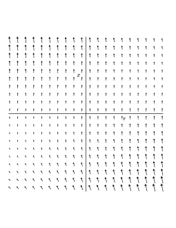
A sketch of his electric field is plotted in Figure 1.
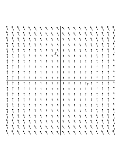
V.2 A Uniform Magnetic Field
Let us consider the case when a uniform magnetic field is present before the passage of the wave. To this end, we need to solve Eq. (61) and, in addition, in order to solve also the homogenous Maxwell’s equation for the magnetic field, we set , where is the vector potential. Accordingly, exploiting the gauge freedom and imposing the Coulomb gauge (), we may write Eq. (61) in the form
| (67) |
where, in this case, from Eqs. (21), (34)-(40), we obtain
| (68) | |||||
On solving Eq. (67), taking into account the vacuum unperturbed solution such that where
| (69) |
we have
| (70) | |||||
| (71) | |||||
| (72) |
and, consequenty the magnetic field has the following components
| (73) | |||||
| (74) | |||||
| (75) |
This magnetic field in the plane is plotted in Figure 1.
VI Discussion and Conclusions
We studied the interaction of a plane gravitational wave with electromagnetic fields. For this purpose we used a formalism that allows Maxwell’s equations in curved spacetime to be written in the form of flat spacetime equations in an effective medium, with appropriate constitutive equations. In particular, we focused on the perturbation induced by a gravitational wave on electromagnetic fields that are present before its passage. Working at first order in the wave amplitude, we showed that the perturbed electromagnetic fields satisfy equations Eqs. (51) and (61), where new terms are present which originate from the coupling of the gravitational field of the wave with the sources of the unperturbed fields and with the unperturbed fields themselves; similar results were obtained by Berlin et al. (2022); Domcke et al. (2022).
To give an idea of the impact of gravitational waves on electromagnetic fields, we considered two simple situations: the case where static and uniform electric and magnetic fields are present. These situations ideally correspond to the field within a capacitor and a within a solenoid. In both cases (see Eqs. (65)-(66) and (73)-(75)) we showed not only that the preexisting fields are perturbed along their initial direction, but also that components in new directions arise. In particular, the perturbations are in the order of
| (76) |
where is the wave amplitude, is the wavelength and is a typical dimension of the measurement device.
We remark that we used a reference frame adapted to the direction of propagation of the wave: namely the axis is the direction of propagation, and is the plane orthogonal to it. In general, the laboratory frame has an arbitrary orientation with respect to the direction of propagation of the wave so we should introduce a set of coordinates that are adapted to the laboratory: this is usually accomplished by using the Euler angles (see e.g. Schutz and Tinto (1987)). However, this would not change the order of magnitude and the physical meaning of the effects that we are studying.
What is the physical interpretation of the modified electric (65)-(66) and magnetic (73)-(75)) fields? We must remember that gravitational waves produce tidal effects, as it is manifest since their impact in the laboratory metric (20) enters through the components of the Riemann tensor. As a consequence, these effects cannot be detected locally, e.g. along the reference world-line, but only by means of a comparison of what happens at different locations in the laboratory frame. To fix ideas, if we consider two identical capacitors, one at the origin of our frame, and the other at the location what we expect is a relative variation of the electric field as described by (65)-(66); the same happens for the magnetic field. As a matter of fact, the passage of gravitational waves also in presence of static electric and magnetic field produce time-varying electromagnetic fields with the same frequency of the waves.
The electromagnetic perturbations determined by the passage of a gravitational wave have the order of magnitude expressed by Eq. (76). To estimate them it is important to remember that the laboratory metric (20) is approximated up to second order in . That being said, and considering that the typical amplitude of gravitational waves reaching the Earth is , we see that relative magnitude of the perturbations can be of the order of . Notice that previous estimates such as those reported by Cabral and Lobo (2017) overestimated the impact of the effect, since they are developed in the TT frame where, however, quantities have not a direct meaning in terms of observables. In any case, as discussed by Cabral and Lobo (2017) (see also references therein), one possibility to detect very small magnetic fields is the use of SQUIDS which can measure magnetic field ranging from T to T Crescini et al. (2022); however, the order of magnitude of the effects we are considering suggests that even using such devices huge unperturbed magnetic field are needed, which are really out of our current technological possibilities. Similar considerations apply to electric fields.
Another kind of approach is the use of resonant cavities (see e.g. Berlin et al. (2022)): the basic idea is that the passage of a gravitational wave affects the shape of a cavity and alters the magnetic flux passing through it, resulting in an electric signal that can be measured. In addition, as we showed, the passage of the wave produces an effective current in Maxwell’s equations, causing an electromagnetic field to oscillate at the same frequency as the gravitational wave. Recent proposals of experimental setups seem quite promising for the detection of gravitational waves Schmieden and Schott (2024).
The general feeling is that, even if current technology does not allow these effects to be measured in terrestrial laboratories, this possibility is not excluded in the future. A completely different scenario is offered by astrophysical events, where the combination of enormous electromagnetic fields and more intense gravitational waves can open up new interesting possibilities; however, this would require a different analysis than the one used in this work as it requires the simultaneous solution of Einstein’s and Maxwell’s equations.
In conclusion, our approach lends itself to a very simple description of the interaction of electromagnetic devices with gravitational waves in terms of observable quantities, and can be used for further studies in this field; the possibility of developing a real experimental proposal is in any case guided by technological developments.
Acknowledgements
The author expresses gratitude to Dr. Antonello Ortolan for engaging discussions and valuable insights. Special appreciation is extended to the local research project "Modelli gravitazionali per lo studio dell’universo" (2022) from the Department of Mathematics "G. Peano," Università degli Studi di Torino, as well as to the Gruppo Nazionale per la Fisica Matematica (GNFM) for their contributions.
References
- Abbott et al. (2016) B. P. Abbott et al. (LIGO Scientific, Virgo), Phys. Rev. Lett. 116, 131103 (2016), arXiv:1602.03838 [gr-qc] .
- Will (2015) C. M. Will, in General Relativity and Gravitation. A Centennial Perspective, edited by A. Ashtekar, B. K. Berger, J. Isenberg, and M. MacCallum (Cambridge University Press, Cambridge, 2015) pp. 49–96.
- Miller and Yunes (2019) M. C. Miller and N. Yunes, Nature 568, 469 (2019).
- Bailes et al. (2021) M. Bailes, B. K. Berger, P. R. Brady, M. Branchesi, K. Danzmann, M. Evans, K. Holley-Bockelmann, B. R. Iyer, T. Kajita, S. Katsanevas, M. Kramer, A. Lazzarini, L. Lehner, G. Losurdo, H. Lück, D. E. McClelland, M. A. McLaughlin, M. Punturo, S. Ransom, S. Raychaudhury, D. H. Reitze, F. Ricci, S. Rowan, Y. Saito, G. H. Sanders, B. S. Sathyaprakash, B. F. Schutz, A. Sesana, H. Shinkai, X. Siemens, D. H. Shoemaker, J. Thorpe, J. F. J. van den Brand, and S. Vitale, Nature Reviews Physics 3, 344 (2021).
- Debono and Smoot (2016) I. Debono and G. F. Smoot, Universe 2 (2016), 10.3390/universe2040023.
- Capozziello and de Laurentis (2011) S. Capozziello and M. de Laurentis, Physics Reports 509, 167 (2011), arXiv:1108.6266 [gr-qc] .
- Rao et al. (2020) S. Rao, M. Brüggen, and J. Liske, Phys. Rev. D 102, 122006 (2020), [Erratum: Phys.Rev.D 105, 069903 (2022)], arXiv:2012.00529 [astro-ph.IM] .
- Rao et al. (2023) S. Rao, J. Baumgarten, J. Liske, and M. Brüggen, (2023), arXiv:2301.08331 [gr-qc] .
- Berlin et al. (2021) A. Berlin et al., in ARIES WP6 Workshop: Storage Rings and Gravitational Waves (2021) arXiv:2105.00992 [physics.acc-ph] .
- Ruggiero and Ortolan (2020a) M. L. Ruggiero and A. Ortolan, Phys. Rev. D 102, 101501 (2020a).
- Berlin et al. (2022) A. Berlin, D. Blas, R. Tito D’Agnolo, S. A. R. Ellis, R. Harnik, Y. Kahn, and J. Schütte-Engel, Phys. Rev. D 105, 116011 (2022), arXiv:2112.11465 [hep-ph] .
- Cooperstock and Faraoni (1993) F. I. Cooperstock and V. Faraoni, Class. Quant. Grav. 10, 1189 (1993), arXiv:astro-ph/9303018 .
- Fortini et al. (1996) P. L. Fortini, E. Montanari, A. Ortolan, and G. Schaefer, Annals Phys. 248, 34 (1996), arXiv:gr-qc/9808080 .
- Montanari (1998) E. Montanari, Class. Quant. Grav. 15, 2493 (1998), arXiv:gr-qc/9806054 .
- Mieling et al. (2021) T. B. Mieling, P. T. Chruściel, and S. Palenta, Class. Quant. Grav. 38, 215004 (2021), arXiv:2107.07727 [gr-qc] .
- Maggiore (2007) M. Maggiore, Gravitational waves: Volume 1: Theory and experiments (OUP Oxford, 2007).
- Synge (1960) J. Synge, Relativity: The General Theory, North-Holland series in physics No. v. 1 (North-Holland Publishing Company, 1960).
- Cabral and Lobo (2017) F. Cabral and F. S. N. Lobo, Eur. Phys. J. C 77, 237 (2017), arXiv:1603.08157 [gr-qc] .
- Landau and Lifshitz (2013) L. D. Landau and E. M. Lifshitz, The classical theory of fields, Vol. 2 (Elsevier, 2013).
- Misner et al. (1973) C. W. Misner, K. S. Thorne, and J. A. Wheeler, Gravitation (San Francisco: WH Freeman and Co., 1973).
- Plebanski (1960) J. Plebanski, Physical Review 118, 1396 (1960).
- Mashhoon (1973) B. Mashhoon, Phys. Rev. D 7, 2807 (1973).
- Leonhardt and Philbin (2006) U. Leonhardt and T. G. Philbin, New J. Phys. 8, 247 (2006), arXiv:cond-mat/0607418 .
- Leonhardt and Philbin (2009) U. Leonhardt and T. G. Philbin, Progess in Optics 53, 69 (2009), arXiv:0805.4778 [physics.optics] .
- Ruggiero and Astesiano (2023) M. L. Ruggiero and D. Astesiano, J. Phys. Comm. 7, 112001 (2023), arXiv:2304.02167 [gr-qc] .
- Ni and Zimmermann (1978) W.-T. Ni and M. Zimmermann, Physical Review D - Particles and Fields 17, 1473 (1978).
- Li and Ni (1979) W.-Q. Li and W.-T. Ni, Journal of Mathematical Physics 20, 1473 (1979).
- Fortini and Gualdi (1982) P. L. Fortini and C. Gualdi, Nuovo Cimento B Serie 71, 37 (1982).
- Marzlin (1994) K.-P. Marzlin, Phys. Rev. D 50, 888 (1994).
- Ruggiero and Ortolan (2020b) M. L. Ruggiero and A. Ortolan, Journal of Physics Communications 4, 055013 (2020b).
- Manasse and Misner (1963) F. Manasse and C. W. Misner, Journal of mathematical physics 4, 735 (1963).
- Mashhoon (2003) B. Mashhoon, in The Measurement of Gravitomagnetism: A Challenging Enterprise, edited by L. Iorio (Nova Science, New York, 2003) arXiv:gr-qc/0311030 [gr-qc] .
- Ruggiero (2021) M. L. Ruggiero, Universe 7, 451 (2021), arXiv:2111.09008 [gr-qc] .
- Rakhmanov (2014) M. Rakhmanov, Classical and Quantum Gravity 31, 085006 (2014).
- Straumann (2013) N. Straumann, General Relativity, With Applications to Astrophysics (Springer, 2013).
- Ruggiero (2022) M. L. Ruggiero, Gen. Rel. Grav. 54, 97 (2022), arXiv:2204.08914 [gr-qc] .
- Domcke et al. (2022) V. Domcke, C. Garcia-Cely, and N. L. Rodd, Phys. Rev. Lett. 129, 041101 (2022), arXiv:2202.00695 [hep-ph] .
- Schutz and Tinto (1987) B. F. Schutz and M. Tinto, MNRAS 224, 131 (1987).
- Crescini et al. (2022) N. Crescini, G. Carugno, P. Falferi, A. Ortolan, G. Ruoso, and C. C. Speake, Phys. Rev. D 105, 022007 (2022), arXiv:2011.07100 [hep-ex] .
- Schmieden and Schott (2024) K. Schmieden and M. Schott, PoS EPS-HEP2023, 102 (2024), arXiv:2308.11497 [gr-qc] .