Simulations of gravitational collapse in null coordinates: II. Critical collapse of an axisymmetric scalar field

Abstract

We present the first numerical simulations in null coordinates of the collapse of nonspherical regular initial data to a black hole. We restrict to twist-free axisymmetry, and re-investigate the critical collapse of a non-spherical massless scalar field. We find that the Choptuik solution governing scalar field critical collapse in spherical symmetry persists when fine-tuning moderately non-spherical initial data to the threshold of black hole formation. The non-sphericity evolves as an almost-linear perturbation until the end of the self-similar phase, and becomes dominant only in the final collapse to a black hole. We compare with numerical results of Choptuik et al, Baumgarte, and Marouda et al, and conclude that they have been able to evolve somewhat more non-spherical solutions. Future work with larger deviations from spherical symmetry, and in particular vacuum collapse, will require a different choice of radial coordinate that allows the null generators to reconverge locally.

I Introduction

In a companion paper paper1 (from now on Paper I), we have reviewed various formulations of the Einstein equations in twist-free axisymmetry on outgoing null cones emanating from a regular centre, intending to simulate gravitational collapse with them.

As a first physics application, here we re-investigate the problem of twist-free axisymmetric scalar field critical collapse. By critical collapse we understand the investigation of the threshold, along a 1-parameter family of initial data, between regular data that do and do not form a black hole in their time evolution. In “type-II” critical collapse, increased fine-tuning to the threshold $p=p_{*}$ gives rise to arbitrarily small black hole masses, arbitrarily large curvatures, and in the limit, it is conjectured, to a naked singularity GundlachLRR .

We choose scalar field critical collapse because it provides a continuous bridge from spherical symmetry, where simulations on null cones work well, to the twist-free axisymmetric vacuum case that is our long-term goal. But it is also of physical interest in its own right.

In JMMGundlach1999 it was claimed, based on the numerical solution of a mode ansatz, that all non-spherical linear perturbations of the spherical scalar field critical solution decay, with the least damped $l=2$ perturbation only decaying quite slowly. Subsequent numerical time evolutions in axisymmetry in cylindrical coordinates by Choptuik et al Choptuiketal2003 appeared to indicate a slowly growing $l=2$ perturbation of slightly non-spherical critical collapse that eventually leads to the formation of two centres of collapse.

This tension between the results of JMMGundlach1999 and Choptuiketal2003 was resolved by fresh simulations, in axisymmetry in spherical coordinates by Baumgarte Baumgarte2018 , which indicated that sufficiently small non-spherical perturbations decay (in agreement with the mode stability claimed in JMMGundlach1999 ) but that larger perturbations do grow (in agreement with Choptuiketal2003 ).

Interestingly, both Choptuiketal2003 and Baumgarte2018 observe that in a regime of small finite deviations from spherical symmetry, the spherical Choptuik solution Choptuik1993 ; MartinGundlach2003 is still observed as an approximate critical solution but with a period that decreases from $\Delta\simeq 3.44$ with increasing non-sphericity, and that the critical exponent also decreases from $\gamma\simeq 0.374$.

The authors of Choptuiketal2003 and Baumgarte2018 , in axisymmetry, achieved fine-tuning to $|p-p_{*}|\sim 10^{-15}$ and $|p-p_{*}|\sim 10^{-13}$, respectively (except that Baumgarte2018 achieved only $10^{-8}$ at the largest deviation from spherical symmetry). Other investigations of non-spherical scalar field collapse had achieved much less fine-tuning: Healeyetal2014 achieved $\sim 10^{-3.5}$, and Deppetelal2019 $\sim 10^{-5.5}$, both for non-axisymmetric initial datap, and CloughLim2016 achieved $\sim 10^{-1}$ in axisymmetry. Incidentally, Healeyetal2014 ; Deppetelal2019 ; CloughLim2016 also evolve initial data that are non-smooth at $R=0$.

Reid and Choptuik Reid2023 have fine-tuned axisymmetric, time-symmetric, antisymmetric in $z$ initial data to $\sim 10^{-14}$ and found that two (mirror-symmetric) centres of collapse form (as one would expect). These start out in a highly non-spherical state (although this was not quantified). However, critical phenomena were observed with $\Delta$ and $\gamma$ as in spherical symmetry, and it was concluded that there is no evidence of a growing non-spherical mode (in the evolution of each separate centre of collapse).

Marouda et al Maroudaetal2024 have examined twist-free axisymmetric collapse of a complex massless scalar field, fine-tuning to $\sim 10^{-10}$. As they treat a slightly different matter model, none of their families of initial data coincides exactly with those of Choptuiketal2003 and Baumgarte2018 , but their results are consistent with those of Choptuiketal2003 and Baumgarte2018 in the sense that $\delta\Delta$ and $\delta\gamma$ observed in their two non-spherical families fit into a monotonic ordering of families by (inferred) non-sphericity. See already Table 2 below.

The achievable level of fine-tuning matters, as the $l=2$ unstable mode claimed in Choptuiketal2003 would be very slowly-growing: its authors see no bifurcation for non-sphericity parameter $\epsilon^{2}\leq 2/3$ [see Eq. (10) below for a definition], but they see one after 2 and 1.5 echos, respectively, for $\epsilon^{2}=3/4$ and $5/6$, where 3 echos is the best that can be achieved in double-precision arithmetic, with $|p-p_{*}|\sim 10^{-15}$. Maroudaetal2024 see about 4 echos in their Family IV before bifurcation.

In principle, being in polar coordinates, our code, as presented in detail in Paper I, should resolve small deviations from spherical symmetry as well as that of Baumgarte2018 , whereas our choice of null gauge should be able to resolve the critical solution well, even without the adaptive mesh refinement of Choptuiketal2003 . It turns out that this is true.

The plan of the paper is as follows: In Sec. II we briefly summarise our metric ansatz, gauge choice and diagnostics, give our two-parameter family (strength and non-sphericity) of initial data, and describe the bisection to the threshold of collapse. In Sec. III we describe in detail our results for spherical critical collapse of a massless scalar field. In particular, we plot the fine structure of the curvature and black hole mass scaling laws with high accuracy and compare with the available literature.

Sec. IV gives our results for non-spherical (twist-free axisymmetric) critical collapse. Our initial data, being set on an outgoing null cones, cannot be compared directly with those of Choptuiketal2003 ; Baumgarte2018 . However, by comparing the amplitude of the $l=2$ deviation of the scalar field $\psi$ from spherical symmetry during the phase of the evolution where the solution is well approximated by the Choptuik solution, we infer that our most non-spherical family, $\epsilon_{2}=0.75$, compares to $\epsilon^{2}=0.5$ of Choptuiketal2003 ; Baumgarte2018 . With the gauge choice presented here we cannot fine-tune families of initial data that are more non-spherical.

We conclude in Sec. V with a discussion of the physical results and an outlook for our code.

II Setup

II.1 Metric and field equations

We state here the equations we solve numerically, with full details of the formulation and its discretization given in Paper I. The field equations we want to solve are the Einstein equations

$$R_{ab}=8\pi\nabla_{a}\psi\nabla_{b}\psi,$$ (1)

and the massless, minimally coupled wave equation

$$\nabla^{a}\nabla_{a}\psi=0.$$ (2)

We use units where $c=G=1$.

We write the general twist-free axisymmetric metric in the form

$$ds^{2} = -2G\,du\,dx-H\,du^{2}$$

$$+R^{2}\left[e^{2Sf}S^{-1}(dy+S\,b\,du)^{2}+e^{-2Sf}S\,d\varphi^{2}\right].$$

We assume that the central worldline $R=0$ is at $x=0$ and that spacetime is regular there. We have defined $y:=-\cos\theta$, so that the range $0\leq\theta\leq\pi$ corresponds to $-1\leq y\leq 1$. The azimuthal angle $\varphi$ has range $0\leq\varphi<2\pi$. The Killing vector generating the axisymmetry is $\partial_{\varphi}$. (We use the convention of equating vector fields with derivative operators.) In (II.1) we have used the shorthand

$$S:=1-y^{2}=\sin^{2}\theta.$$ (4)

Each surface ${\cal N}^{+}_{u}$ of constant $u$ is an outgoing null cone, assumed to have a regular vertex. Each surface ${\cal S}_{u,x}$ of constant $u$ and $x$ is assumed to be spacelike, and has topology $S^{2}$. The outgoing future-directed null vector field normal to ${\cal S}_{u,x}$ is $U:=G^{-1}\partial_{x}$, and is also tangent to the affinely parameterised generators of ${\cal N}^{+}_{u}$. The ingoing future-directed null vector normal to ${\cal S}_{u,x}$ is

$$\Xi:=\partial_{u}-B\partial_{x}-Sb\partial_{y},$$ (5)

where we have defined the shorthand

$$B:={H\over 2G}.$$ (6)

As we see from (5) $B$ plays the role of a “shift” in the $x$-direction, with $B$ and $b$ relating our time direction $\partial_{u}$ to the ingoing null direction $\Xi$. $U$ and $\Xi$ are normalised relative to each other as $\Xi^{a}U_{a}=-1$. See Fig. 1 of Paper I for a sketch of our coordinate null cones and these vector fields.

As described in Paper I, we can solve a subset of the Einstein equations and the wave equation (which we call the hierarchy equations) for $G$, $b$, $\Xi R$, $\Xi f$ and $\Xi\psi$ on one time slice, given $R$, $f$ and $\psi$ there, and this can be done by explicit integration in $x$ in the right order. $H$ and $\partial_{u}$ do not appear in the hierarchy equations except in the combination $\Xi$, and $H$ remains undetermined.

This means that we have a time evolution scheme where $R$, $f$ and $\psi$ are specified at $u=0$. We then find $G$, $b$, $\Xi R$, $\Xi f$ and $\Xi\psi$ , choose $B$ freely and thus obtain $R_{,u}$, $f_{,u}$ and $\psi_{,u}$, and then evolve $R$, $f$ and $\psi$ forward in $u$.

We discretize in $x$ and $u$ using finite differencing, and in $y$ using a pseudospectral expansion in Legendre polynomials (that is, spherical harmonics restricted to axisymmetry).

II.2 Gauge choice

Our numerical domain is $0\leq x\leq x_{\text{max}}$, $0\leq u\leq u_{\text{max}}$. We choose $H$ within a class of gauge choices with the property that $R=0$ remains at $x=0$ (and is timelike and regular), and that $x=x_{\text{max}}$ is future spacelike. This means that our numerical domain is a subset of the domain of dependence of the initial data on $0\leq x\leq x_{\text{max}}$, $u=0$, and no boundary condition is required on the outer boundary $x=x_{\text{max}}$. We set $H=G=1$ at $x=R=0$, so that the proper time along this “central wordline” is given by $u$.

Furthermore, we impose that $x=x_{0}$ is marginally future spacelike, in the sense that $H(u,x_{0},y)\leq 0$, with equality for some $y$, for some fixed constant $x_{0}$ in the range $0<x_{0}\leq x_{\text{max}}$. Our expectation is that, if a part of the spacetime we are constructing numerically is approximated by a self-similar critical spacetime (with accumulation point on the central worldline $x=0$), then we can (by trial and error) adjust $x_{0}$ so that $x=x_{0}$ remains close to the past lightcone of the accumulation point of scale echos. The resulting coordinate system will then zoom in on the accumulation point and maintain resolution of the ever smaller spacetime features as it is approached, without the need for adaptive mesh refinement. This approach to critical collapse in null coordinates was used in Garfinkle1995 ; ymscalar , using regridding, and in Rinne2020 ; PortoGundlach2022 using a shift term, all in spherical symmetry.

More specifically, for this paper we have settled on a class of gauges we call “local shifted Bondi gauge” (from now on, lsB gauge), defined by $R(u,x,y)=\bar{R}(u,x)$. Within that class, we choose the “lsB4” flavour, defined by the shift $B$ defined in (6) taking the value

$$B_{\text{lsB4}}=-{\Xi R-\min_{y}(\Xi R)\over R_{,x}}+\left(1-{x\over x_{0}}\right)\left(-{\Xi R\over R_{,x}}\right)_{x=0}.$$ (7)

(Note that in Paper I we extensively tested the slightly different lsB2 gauge.) In this gauge, every surface of constant $x>x_{0}$ is future spacelike. We refer the reader to Paper I for more details. Note that $B(u,x,y)$ is continous but has discontinuous transverse derivative across the hypersurfaces $x=x_{*}(u)$ where the $y$-location of $\min_{y}(\Xi R)$ jumps.

II.3 Diagnostics

For any closed spacelike 2-surface ${\cal S}$, we define its “Hawking compactness”

$$C({\cal S}):=1+{1\over 2\pi}\int_{\cal S}\rho_{+}\rho_{-}\,dS,$$ (8)

where $\rho_{+}$ and $\rho_{-}$ are the outgoing and ingoing null divergence. It is related to the well-known Hawking mass by

$$M({\cal S}):={1\over 2}\sqrt{A({\cal S})\over 4\pi}\,C({\cal S}),$$ (9)

where $A({\cal S})$ is the area of ${\cal S}$.

The standard indicator of black hole formation used in numerical relativity on a spacelike time slicing is the appearance of a marginally outer-trapped surface (from now on, MOTS) embedded in a time slice. An outer trapped surface is defined by $\rho_{+}\leq 0$ at every point (and hence $C>1$), and a MOTS by $\rho_{+}=0$ (and hence $C=1$). As we have discussed in Paper I, we cannot expect the ingoing past light cone of a MOTS to converge to a point, and so we cannot expect to find any MOTS embedded in a coordinate null cone.

Instead we use the Hawking compactness $C(u,x)$ of our coordinate 2-surfaces ${\cal S}_{u,x}$ as an indicator of black-hole formation. When $\max_{x}C(u,x)\geq 0.99$ is first reached during an evolution, we use the Hawking mass $M$ of the ${\cal S}_{u,x}$ where that happens as an indication of the “initial mass” of the black hole. Similarly, we use $\max_{x}C(u,x)\leq 0.01$ as an indicator of dispersion. In spherical symmetry, this works perfectly well: $C=1$ is actually equivalent to a MOTS, and this MOTS is approached uniformly at all angles $(\theta,\varphi)$. Beyond spherical symmetry, for current lack of a better alternative, we still use $C(u,x)$ to distinguish between dispersion and collapse.

However, $C({\cal S})\geq 1$ is clearly only necessary, not sufficient, for ${\cal S}$ to be outer-trapped, and we are not aware of any rigorous results linking 2-surfaces with $C\simeq 1$ to black holes, nor of their previous use in the numerical relativity literature beyond spherical symmetry.

In lsB gauge, where $R=\bar{R}(u,x)$, the Hawking mass $M(u,x)$ of the coordinate 2-surfaces ${\cal S}_{u,x}$ obeys $M_{,x}(u,x)\geq 0$. There are separate integrals for $C(u,x)$ and $M(u,x)$, and this gives to two separate ways of computing $C$, whose numerical results we denote by $C$ and $\tilde{C}$, and similarly $M$ and $\tilde{M}$. Their agreement is strong test of numerical accuracy, as they are discretised in different ways, see Paper I for details.

II.4 Initial data

The authors of Choptuiketal2003 investigate non-spherical scalar field collapse in axisymmetry, using two families of initial data on a Cauchy surface. One is time-symmetric, with the initial value of the scalar field a Gaussian elongated along the rotation axis, with equatorial symmetry. The other is approximately ingoing, with $\psi$ antisymmetric under reflections through the equator. Like the code of Baumgarte2018 , ours is optimised for a single centre of collapse, while the antisymmetric data have two, so we evolve only a family of data designed to be similar to the first family of Choptuiketal2003 .

The time-symmetric initial data of Choptuiketal2003 and Baumgarte2018 at $t=0$, written in our notation, are

$$\phi(0,r,y)=p\,e^{-{r^{2}(1-\epsilon_{2}y^{2})\over d^{2}}},\qquad\phi_{,t}(0,r,y)=0.$$ (10)

With $\epsilon_{2}>0$, the initial data are elongated along the symmetry axis $y=\pm 1$, and with $\epsilon_{2}<0$ they are squashed. In Choptuiketal2003 ; Baumgarte2018 , $\epsilon_{2}$ is written as $\epsilon^{2}$ and only positive values are considered, but there is no reason not to consider $\epsilon_{2}<0$, hence our change of notation. Given the initial data for the scalar field, Choptuiketal2003 ; Baumgarte2018 obtain full initial data for the Einstein-scalar system by making the initial 3-metric conformally flat and solving the Hamiltonian constraint for the conformal factor.

As we set initial data on an outgoing null cone $u=0$ rather than a time slice $t=0$, we cannot construct initial data giving exactly the same solutions. As an approximate equivalent, we consider the function

$$\phi(t,r,y) := {1\over 2r}\Bigl{[}(t+r)e^{-{(t+r)^{2}\over d^{2}}(1-\epsilon_{2}y^{2})}$$ (11)

$$-(t-r)e^{-{(t-r)^{2}\over d^{2}}(1-\epsilon_{2}y^{2})}\Bigr{]}.$$

For $\epsilon_{2}=0$ only, this a spherically symmetric analytic solution of the scalar wave equation on flat spacetime. For any $\epsilon_{2}$, it also reduces to (10) at $t=0$. In our null code, we now set the free initial data at $u=0$ to

$$\psi(0,R,y)=p\,\phi(t_{0}+R,R,y)$$ (12)

for some constant $t_{0}$, so that $u=0$ corresponds to $t=t_{0}+R$. We also set

$$f(0,x,y)=0.$$ (13)

This is simply for lack of an alternative likely to be closer to the corresponding data at $t=0$ being conformally flat, and is at least consistent with spacetime being flat in the limit $p\to 0$. Finally, we set

$$R(0,x,y)={x\over 2},$$ (14)

which is essentially a gauge choice.

Formally, as $p\to 0$ and $\epsilon_{2}\to 0$, the solution from these data corresponds to that arising from (10), with the identification $u=t-R$. We also initialise $R(0,x,y)=x/2$, which can be considered our initial choice of an lsB gauge.

Obviously, with gravity and/or with $\epsilon_{2}\neq 0$, (11) is no longer an exact solution of the curved-spacetime wave equation, and the solution evolved from the null initial data (12) no longer has a moment of exact time symmetry, but it should approximate the solutions arising from (10), with $\epsilon_{2}$ playing a quantitatively similar role.

Without loss of generality we set $d=1$ to fix an overall scale. We also choose $t_{0}=-5$, which means that the null initial data (12) represents a Gaussian that is well separated from the centre and still essentially ingoing. In the flat-space, spherical limit $\epsilon_{2}=0$, $p\to 0$ the wave reaches the centre at $u=-t_{0}$, and the moment of time symmetry $t=0$ corresponds to $u+R=-t_{0}$. Hence (always in this limit) our null initial data $u=0$ intersect $t=0$ at $R=-t_{0}$. For $\epsilon_{2}=0$, we shall choose $x_{\text{max}}=11$, so that $R=-t_{0}$ intersects our initial data surface.

We realised only near the completion of this paper, from the convergence tests in Appendix B, that for $\epsilon_{2}\neq 0$ and $t\neq 0$ (11) is not actually single-valued at the origin $r=0$, but depends on $y$. Our null initial data (12) are therefore also not single-valued at the origin. In Appendix C we present an analytic solution of the flat space wave equation valid for all values of $\epsilon_{2}$ that also reduces to (10) for all values of $\epsilon_{2}$, and null initial data (38) derived from this solution. These are the initial data we intended to create.

However, convergence tests in the strong-gravity regime of the non-analytic null data (12) with (11) show that the breakdown of convergence is limited to a small region near the origin, at early times. The code seems to smooth out the data to something that then converges. The corrrected null data (38) also converge, but preliminary tests show that at $\epsilon_{2}=0.75$ they require very large values of $x_{\text{max}}$ in near-critical evolutions. For both these reasons — the error in the non-analytic data does not seem to matter, and the analytic data are much harder to evolve — we present here only evolutions with the non-analytic initial data, and we believe that the following results are still reliable.

II.5 Bisection to the threshold of black hole formation

Beginning from a value of $p$ that disperses and one that collapses, we find the threshold value $p_{*}$ by bisection. We use super$n$ as shorthand for $\ln(p-p_{*})\simeq-n$ and sub$n$ for $\ln(p_{*}-p)\simeq-n$. (This makes sense because $p$ is dimensionless and $p_{*}\sim 1$.) We can find $p_{*}$ to machine precision (15 digits), and the accumulation point of echos $u_{*}$ to about 7 digits, but our numerical values of $p_{*}$, $u_{*}$ and $x_{*}$ will agree with their continuum value to fewer digits. This is a well-known feature of numerical simulations of critical collapse. Below we give their values at different resolutions as a rough indication of numerical error.

Beyond spherical symmetry, during bisection in $p_{*}$, or later when we sample $\ln|p-p_{*}|$ more finely, we occasionally obtain inconclusive evolutions. For small $\epsilon_{2}$ at least there is a heuristic workaround: when the evolution stops as the time step goes below an acceptable threshold, we always find that $\max_{x,y}\rho_{-}>0$ as well. We take this combination as an indicator of collapse, even if $C=0.99$ has not yet been reached. At the largest non-sphericity and highest resolution, this collapse criterion also fails, and we replace it by $\max_{x}C(u,x)\geq 0.8$.

We cannot be sure that what we thus classify as collapse or dispersion really is, but if we then see subcritical curvature scaling on the “dispersion” side, and approximate self-similarity on both sides, we take this to be a strong indication that we really are bisecting to the collapse threshold. Furthermore, any mass-like quantity in near-critical evolutions will also scale, in particular the Hawking mass on the first surface ${\cal S}_{u,x}$ where $C=0.99$ (or $C=0.8$), and seeing this scaling at least provides further confirmation that we are bisecting to the black hole threshold, even if the mass we measure is related to the black hole mass only by a factor of order one.

Once we have an estimate for $p_{*}$ (which depends on all the numerical parameters), we evolve super and subcritical values of $p$ that are equally spaced in $\ln|p-p_{*}|$, with 30 values per power of 10, to give us better-resolved plots of the mass and curvature scaling laws.

III Results in spherical symmetry

We begin with the spherical case $\epsilon_{2}=0$, and run with $N_{y}=1$ in lsB4 gauge. By experimentation we find that $x_{0}=8.24$ allows bisection down to machine precision, while keeping the first appearance of $C\geq 0.99$ somewhere in the middle of the grid as the bisection proceeds (in order to resolve the critical solution). In other words, the past lightcone of the accumulation point of scaling echos is at $x_{*}\simeq 8.24$. We also find that $x_{\text{max}}=11$ is required in order to capture the location where $C$ first reaches the threshold value of $0.99$ that we take as an indication of collapse. We find $p_{*}\simeq 0.2402$.

We have checked that our code shows clean pointwise second-order convergence with $\Delta x$ in the two evolutions forming our initial bracket: the clearly subcritical $p=0.2$, and the clearly supercritical $p=0.3$ (up to a little before our collapse criterion stops the supercritical evolution).

As a basic check, we have evolved spherically symmetric initial data also with $\bar{N}_{y}=3$. This makes no visible difference to the scaling plots or critical solution (except where they dissolve into round-off noise). However, round-off error in the spectral operations triggers unphysical random nonspherical perturbations. These are then smoothed out by the shrinking of the numerical grid, and then, once their $x$-dependence is resolved, continue to evolve under the continuum perturbation equations. The $l=2$ spherical harmonic components of $\psi$ and $f$, which from now on we shall denote $\psi_{2}$ and $f_{2}$, reach an amplitude $\sim 10^{-12}$ and then decay in sub15, while they blow up in super15 during the final collapse. This blowup may be explained by the physical instability of gravitational collapse to non-spherical perturbations, even if these perturbations were triggered here by numerical error.

We stop the bisection to $p_{*}$ after 50 iterations, where we are essentially at machine precision. However, the scaling laws for the initial black hole mass and maximum Ricci curvature become noisy well before we reach machine precision, at about sub13 for the the Ricci scaling (see Fig. 1) and at about super12 for the mass scaling (see Fig. 2).

In spherical symmetry and evolving with $N_{y}=1$, the source of the randomness is presumably round-off error, becoming important in the evolutions already three or so orders of magnitude before we reach machine precision in $p$ itself.

III.1 Fine structure of the mass and curvature scaling laws

From Appendix A, which clarifies the derivation given in Gundlach1997 , we expect the scaling laws

$$-{1\over 2}\ln T \simeq A+\gamma\ln(p_{*}-p)$$ (15)

$$+f_{T}\left(\ln(p_{*}-p)+B\right),$$

$$\ln M \simeq A+\gamma\ln(p-p_{*})$$ (16)

$$+f_{M}\left(\ln(p-p_{*})+B\right),$$

for

$$T:=\max_{\text{whole spacetime}}|\nabla_{a}\psi\nabla^{a}\psi|,$$ (17)

and the mass $M$ of the first MOTS detected on our time slicing. We consider $T^{-1/2}$ because it has dimension length, like $M$, and we use the natural logarithm for all our plots. Here $\Delta\simeq 3.44$ and $\gamma\simeq 0.374$ are universal constants, and $A$ and $B$ are family-dependent constants. $f_{T}$ is a universal periodic function with period $\Delta/(2\gamma)\simeq 4.60$ in $\ln(p_{*}-p)$. $f_{M}$ is also periodic with the same period, and is universal with respect to initial data in a given DSS-compatible time slicing (such as our null cone slicing), but does depend on the slicing, as well as our collapse criterion.

Note that the Ricci scalar is $|\text{Ric}|=8\pi T$, so $\ln|\text{Ric}|$ and $\ln T$ differ only by a constant.

To look for these scaling laws, we plot $\ln M-(A+\gamma\ln|p-p_{*}|)$ against $\ln\ln|p-p_{*}|$, and similarly for $T$. We then expect to see only the fine-structures $f_{M}$ and $f_{T}$. To uniquely fix $A$ for a given family, we define $f_{T}$ to have zero mean. To fix $B$ modulo periodicity, we let the minima of $-(1/2)\ln T$ coincide with the minima of $\sin(\gamma\ln|p_{*}-p|)$. We find that for our family of spherical initial data $A\simeq 1.113$, $B=0.592$, $\gamma=0.374$ and $\Delta=3.44$ provide a good fit to (15) for our family of spherically symmetric initial data.

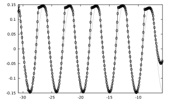
Figure 1: $\epsilon_{2}=0$: Numerical determination of the curvature scaling function $f_{T}$. Here and in all following plots of $f_{T}$, the horizontal axis shows $\ln(p_{*}-p)+B$ and the vertical axis shows $-1/2\ln T-A$. To make the plots larger, we omit axis labels in all line plots throughout. Circles indicate our data points, 30 per decade in $p-p_{*}$. We show only the range where the function is approximately periodic. The grey line represents a fit as a sine wave of amplitude $0.147$. For comparison, in all following plots of $f_{T}$ and $f_{M}$ the range of $\ln(p_{*}-p)+B$, will be the same as here, namely $[-30.8,-5.8]$.

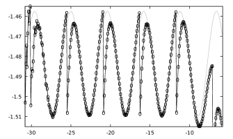
Figure 2: $\epsilon_{2}=0$: Numerical determination of the mass scaling function $f_{M}$. Here and in all following plots of $f_{M}$, the horizontal axis shows $\ln(p-p_{*})+B$ and the vertical axis shows $\ln M-A$. The grey line represents a fit as $-1.4835$ plus a sine wave of amplitude $0.026$. $f_{M}$ is strictly periodic over a slightly smaller range than $f_{M}$.

Our numerical measurement of $f_{T}$ with these fitting parameters is shown in Fig. 1. We see accurate periodicity from sub2.5 to sub13. The function $f_{T}$ is well approximated by a fundamental sine wave of amplitude $0.147$, except for a widened top and a clear discontinuity in the derivative at the left edge of this flattened top. This kink is expected: it corresponds to the appearance of a new local maximum of $T$ in each scale period.

Our numerical measurement of $f_{M}$ is shown in Fig. 2. Recall that $M$ is the Hawking mass of the first surface ${\cal S}_{u,x}$ with Hawking compactness $C=0.99$. $f_{M}$ is periodic with an amplitude of about $0.026$ and mean $-1.4835$. There is one large discontinuity in each period, corresponding to the formation of the first MOTS one scale period later. Again this is expected: when a new local maximum of $C$ takes over, by definition it has the same $C$, but not the same $M$. We see accurate periodicity with the same $\gamma$ and $\Delta$ as for the curvature scaling law, over a slightly smaller range from sub4 to sub12. The range may be smaller because the MOTS occurs near the past light cone of the singularity of the underlying critical solution, whereas the maximum of the Ricci curvature occurs at the centre, which may be less affected by details of the initial data.

We are aware of the following previous plots of scaling law fine-structures in the critical collapse of a spherical scalar field in the literature.

Pürrer, Husa and Aichelburg PuerrerHusaAichelburg extend compactified Bondi coordinates to future null infinity, and so can read off the asymptotic black hole mass. They show a periodic fine structure of this mass which appears to be continuous, with an amplitude of about $0.4$ in $\ln M$. Crespo, Oliveira and Winicour CrespoOliveiraWinicour2019 use an affine radial coordinate also compactified to null infinity and show a similar fine structure, but with an amplitude that seems to be closer to $0.3$ in $\ln M$. These results are in the same time slicing, so they should agree, and they roughly do. From a plot in Rinne Rinne2020 we estimate the amplitude in $\ln M$ as $\simeq 0.4$, similar again to PuerrerHusaAichelburg ; CrespoOliveiraWinicour2019 , although this is not the asymptotic mass. By contrast, our $f_{M}$ has an amplitude of only $0.026$ in $\ln M$, and has a jump of similar amplitude. Our best guess is that the Hawking mass of our collapse diagnostic is still very far from the final black hole mass. We have explained why our $f_{M}$ is discontinous, but by contrast we have no theoretical understanding of why the $M(p)$ measured by the other researchers is continuous.

Switching now to the subcritical scaling of the maximum of the Ricci curvature, Garfinkle and Duncan GarfinkleDuncan1998 plot the fine-structure in $\ln\max|\text{Ric}|$, and from this plot we estimate the amplitude of $f_{T}$ as $0.3$ in $\ln\max|\text{Ric}|$, or $0.15$ in $(1/2)\ln\max|T|$. This is consistent with our value of $0.147$. The bottom of their curve, corresponding to the top of ours, is flattened, again consistent with our observation. Baumgarte Baumgarte2018 has a fine-structure with amplitude of about $0.35$ in $\ln\max\rho$, where $\rho=n^{a}n^{b}T_{ab}$ is the energy density measured by an observer normal to the time slicing. This depends on the slicing, but the amplitude of $0.35$ is again similar to the $0.3$ observed by us and GarfinkleDuncan1998 for $\ln\max|\text{Ric}|$.

III.2 Self-similarity of the critical solution

We demonstrate self-similarity of the critical solution by showing that the scalar field $\psi$, the compactness $C$ and the scaled curvature scalar

$${\cal T}:=(u_{*}-u)^{2}|\nabla_{a}\psi\nabla^{a}\psi|$$ (18)

are periodic in the DSS-adapted coordinates

$$\xi := {R\over u_{*}-u},$$ (19)

$$\tau := -\ln(u_{*}-u).$$ (20)

The null slicing is already DSS-compatible, in the sense of Corsetal2023 , but we call this specific coordinate system DSS-adapted as the parameter $u_{*}$ needs to be adjusted to the accumulation point of the specific DSS. Unlike the scalar field, the metric actually has period $\Delta/2$ because the Choptuik solution has the property that $\psi_{*}(\xi,\tau+\Delta/2)=-\psi_{*}(\xi,\tau)$ and $R_{ab}=8\pi\psi_{,a}\psi_{,b}$ is invariant under $\psi\to-\psi$. The parameter $u_{*}$ is a family-dependent constant. A rough initial guess of $u_{*}$ is given by the time that near-critical supercritical evolutions stop. We then refine it by making $\psi$, $C$ and ${\cal T}$ as periodic as possible. For our family, we find $u_{*}\simeq 5.609$.

Note that adjusting $u_{*}$ slightly will affect $\tau(u)$ the more the closer $u$ gets to $u_{*}$. In practice, we can therefore adjust the $\tau$-location of the last echo of, say, $\psi(x,\tau)$ by adjusting $u_{*}$, almost without moving the other echos. By contrast, this arbitrariness is absent when we use $u_{*}$ to make the amplitude of the last echo of ${\cal T}(x,\tau)$ equal to that of the preceding echos, and is therefore what we use to determine $u_{*}$.

We use our closest super- and subcritical evolutions as a proxy for the critical solution. They agree with each other until one disperses and the other one forms a black hole. We see clear echoing in $\psi$, $C$ and ${\cal T}$ for $2\lesssim\tau\lesssim 10$. The results are shown in Figs. 3, 4 and 5 for our closest subcritical evolution.

Figure 3: $\epsilon_{2}=0$: Surface plot of the scalar field $\psi(x,\tau)$ against the similarity coordinates $\xi$ and $\tau$, in our closest subcritical evolution (sub15). The plot has been cropped to $0\leq\xi\leq 1$, but the entire range of $\tau$ is shown, starting from the initial data at $u=0$ at the right edge of the plot, and ending at the left edge when $C\leq 0.01$ indicates dispersion. The centre is at $\xi=0$ (front edge), and the past lightcone of the singularity at $\xi\simeq 1$ (back edge). Approximate DSS is seen for the range $2\lesssim\tau\lesssim 10$. Our numerical data form a mesh made up of lines of constant $u$ (constant $\tau$) and constant $x$ (not constant $\xi$). Both have been down-sampled for visual clarity.

Figure 4: $\epsilon_{2}=0$: Surface plot of the compactness $C$, otherwise as described in Fig. 3.

Figure 5: $\epsilon_{2}=0$: Surface plot of the scaled curvature diagnostic ${\cal T}$, otherwise as in Fig. 3, except that the plot has been rotated slightly to the right for a clearer view.

III.3 Comparison with gsB gauge

We have also bisected $\epsilon_{2}=0$, $N_{y}=1$ in “global shifted Bondi” (gsB) gauge. Recall from Paper I that this is given by $R=s(u)x$, giving

$$\left(B\right)={\dot{s}(u)x-\Xi R\over s(u)},$$ (21)

and we have settled on the particular flavor given by

$$\dot{s}(u)={1\over x_{0}}\min_{y}\Xi R(u,x_{0},y).$$ (22)

We needed $x_{\text{max}}=20$ in gsB gauge (instead of $11$ in lsB gauge), and correspondingly $N_{x}=800$ to maintain $\Delta x=0.025$. Comparing the zoomed-in scaling laws with lsB and gsB, they agree as expected down to about super/sub12, but then begin to disagree as both become noisy.

In spite of this apparent success, we see a fundamental problem with gsB gauge already here in spherical scalar field collapse. While $B$ is a monotonically decreasing function in weakly curved spacetimes, going through $B=1$ at $x=0$ and $B=0$ at $x=x_{0}$, in near-critical spacetimes it becomes non-monotonic and may cross zero at $x=x_{0}$ with positive slope. This means that some surfaces of constant $x>x_{0}$ are no longer future spacelike but timelike. This could include the outer boundary, and we would then not evolve on the domain of dependence. It is possible that $B$ becomes negative again for sufficiently large $x$ , and indeed this happens for $x_{\text{max}}=20$ in this family of spherical initial data, but it is not something we can rely on.

Given that the only free parameter of gsB gauge is $x_{0}$, and that this needs to be set to $x_{*}$, which in turn is set by the family of initial data, in order to resolve the critical solution this seems to be a fundamental problem with gsB gauge. Indeed, gsB gauge fails for this reason in nonspherical evolutions, and we present no results in this gauge.

IV Results for nonspherical initial data

As already noted, the strong-field convergence tests with $\epsilon_{2}=0.75$ in Appendix B showed an initial burst of non-convergent error caused by our initial data not being analytic at the origin, but we see second-order convergence with $\Delta x$ and $l_{\text{max}}$ for all $u\gtrsim 0.2$. Here we present results for these non-analytic initial data, as we believe the initial error does not affect our results in the critical regime.

We have bisected in the families with $\epsilon_{2}=0$, $10^{-4}$, $10^{-2}$, $0.1$, $0.5$ and $0.75$, using lsB4 gauge. Note our family of null data parameterised by $(p,\epsilon_{2})$ is equivalent to the family of Cauchy data parameterised by $(p,\epsilon^{2})$ of Choptuiketal2003 ; Baumgarte2018 only in the limit of small $\epsilon_{2}$ and small $p$, as we rely on a spherically symmetric solution of the wave equation on flat spacetime to relate the scalar $\psi$ field at $t=0$ to $u=0$. Table 1 lists the numerical parameters and outcomes of our successful bisections. To estimate the error from discretization in $x$ and $y$, we have run $\epsilon_{2}=0.75$ at four resolutions, with $\Delta x=0.05$ and $0.025$, and $\bar{N}_{y}=9$ and $17$ for both. However, because of the large number of long evolutions involved, we have not plotted the fine structures of the scaling laws for the combination of the two higher resolutions. Moreover, at higher fine-tuning during the bisection, we had to reduce our criterion for collapse from $C\geq 0.99$ to $C\geq 0.8$. This would of course affect the mass scaling law (if we computed it), but appears to be sufficient for the bisection, and hence finding the approximate critical solution.

From (11), we expect that for sufficiently small $\epsilon_{2}$, the non-sphericity evolves as a linear perturbation of spherical symmetry, dominated by $l=2$, and that this linear perturbation decays. For somewhat larger $\epsilon^{2}$, Choptuiketal2003 ; Baumgarte2018 also found changes to $\Delta$ and $\gamma$. For even larger $\epsilon^{2}$, in particular $\epsilon^{2}=0.75$, Baumgarte Baumgarte2018 also found evidence of the (nonlinear) instability of the Choptuik solution reported by Choptuik et al Choptuiketal2003 to lead to two centres of collapse. We will see, by contrast, that for our $\epsilon_{2}=0.75$ evolutions the nonspherical perturbations appear to still be in the linear regime, and indeed their non-sphericity is more similar to the evolutions of Baumgarte Baumgarte2018 with his $\epsilon^{2}=0.5$.

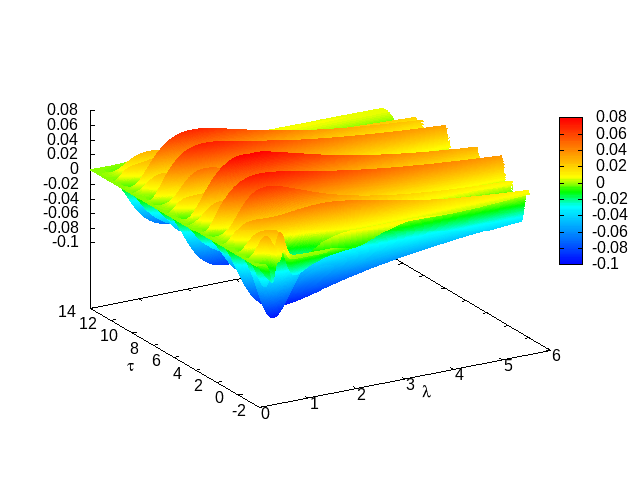
Figure 22: Surface plot of $(3/2)/\epsilon_{2}\psi_{2}\simeq\delta\psi/\epsilon_{2}$ for $\epsilon_{2}=10^{-2}$ against similarity coordinates $\tau$ and $\xi_{\lambda}$. This should be compared to Fig. 11 of Baumgarte2018 . The colour map has been chosen purely for visual agreement with that figure. The range of $\xi_{\lambda}$ is the same as there, but our range of $\tau$ is larger, $[0,14]$ rather than $[0,8]$, as we can fine-tune more closely to the black hole threshold.

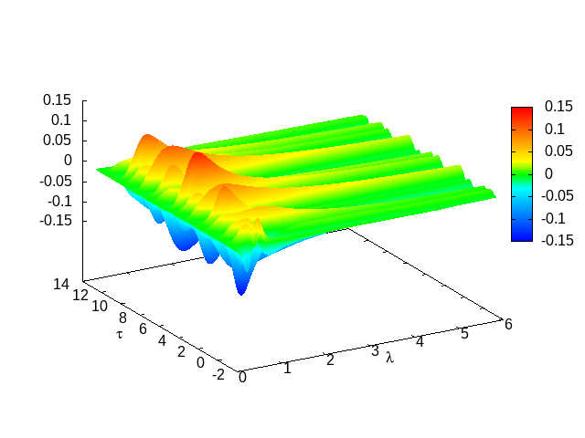
Figure 23: As in Fig. 22, but for $\epsilon_{2}=0.75$

$\epsilon_{2}$	$\Delta x$	$\bar{N}_{y}$	$l_{\text{max}}$	$x_{0}$	$x_{\text{max}}$	$p_{*}$	$u_{*}$	$A$	$B$	comments
0	0.025	1/3	0/4	8.24	11.	0.2402	5.609	1.113	0.592	no filtering, Figs. 1-7, 12-13
$10^{-4}$	*	9	8	*	*	*	*	*	*	Figs. 12-13
$10^{-2}$	*	3/5/9	2/4/8	8.275	15.	*	5.610	1.115	*	Figs. 6-9, 12-15, 18-19, 22
0.1	*	3/5/9	2/4/8	8.7	*	0.2406	5.620	1.131	*	Figs. 6-7, 12-15, 18-19
0.5	*	5/9	4/8	12.5/13.3	*	0.2452	5.657	1.230	0.737	*
0.75	0.05	9	8	24.	50.	0.2555	5.642	1.250	1.059	Figs. 10-11
	*	17	16	30.	*	0.2556	*	*	*	*
	0.025	9	8	24.5	*	0.2535	5.651	*	*	*
	*	17	16	33.	*	*	5.652	*	*	$C\geq 0.8$, Figs. 6-7, 10-21, 23

Table 1: Table showing parameters of our families of initial data. $\epsilon_{2}$, in the first column, is the only physical input parameter. The second group group of columns shows numerical (input) parameters, and the third group physical (observed) parameters (fitted to the numerical data, and rounded to four significant digits for this table). These families, or the best subcritical evolutions in them, have been used in the figures listed in the last column. For visual clarity, a * means the entry is unchanged from the previous row. Half-frequency filtering was applied except in the first row, and the collapse criterion was $C\geq 0.99$ except in the last row, where it was $C\geq 0.8$.

IV.1 The final collapse phase

Our best supercritical evolution remains, by definition, close to our best subcritical one until the end when one decides to disperse and the other to collapse. However, in its final collapse phase the best supercritical solution becomes much more non-spherical, and this is challenging numerically.

In flat spacetime $\Xi R=-1/2$, $R\rho_{+}=1$ and $2R\rho_{-}=-1$. By contrast, in critical collapse, the divergence $\rho_{+}$ of the outgoing null geodesics remains approximately spherical and positive in the self-similar phase, but in the final collapse becomes very small at large $x$. Similarly, $\rho_{-}$ and $\Xi R$ remain negative and approximately spherical in the self-similar phase, but become very large, and positive for a range of angles intermediate between the poles and equator, in the final collapse phase.

We also see a fundamental numerical challenge of highly nonspherical evolutions in lsB gauge: The $x$-shift $B$ in

$$\bar{R}_{,u}=\Xi R+BR_{,x}$$ (23)

tries to counteract the non-spherical part of $\Xi R$ to keep $R$ independent of $y$ but has little to act on as $R_{,x}\to 0$, while $\Xi R$ also becomes larger. Therefore $B$ becomes large, and by the Courant condition applied to the upwinded shift terms, the time step becomes small. In spherical symmetry this is less of a problem because $R_{,x}\to 0$ also indicates an approaching MOTS, whereas in a non-spherical spacetime it does not.

Another consequence of the asphericity of the final collapse phase is that we do not then have sufficient angular resolution to obtain reliable values for $M$. In the continuum $\tilde{C}=C$ and $\tilde{M}=M$, but in the final collapse phase their numerical values differ strongly. There is little hope that we can overcome this problem with more angular resolution, as physically we expect the ${\cal S}_{u,x}$ to become arbitrarily non-spherical inside the black hole. As a heuristic indicator of collapse for the purpose of bisecting to the black hole threshold, we therefore use $\tilde{C}$ rather than $C$, as $\tilde{M}$ is at least non-decreasing by construction. Of course either $\tilde{M}$ or $M$ should be considered reliable only to the extent they agree with each other.

IV.2 Scaling and echoing

We look for three types of evidence that the non-spherical perturbations are in the linear regime: for sufficiently small $\epsilon_{2}$, the spherical part of the critical solution should be the same critical solution as for $\epsilon_{2}=0$, and its perturbations should decay and oscillate as predicted by linear perturbation theory about the spherical critical solution. The growth rate $\lambda_{0}>0$ of the unique growing mode should be unchanged, and hence the scaling laws, including $\gamma$, $f_{T}$ and $f_{M}$ should be as for $\epsilon_{2}=0$. Finally, the decay rates $\lambda$ of the leading perturbation modes should be independent of $\epsilon_{2}$ for $\epsilon_{2}$ sufficiently small, with the values predicted in perturbation theory in Gundlach1997 . We examine evidence for all this in the next two subsections, starting here with the scaling laws.

Fig. 6 and Fig. 7 compare the fine structures of $T^{-1/2}$ and $M$ scaling, respectively, for different $\epsilon_{2}$, using our highest resolution data at each $\epsilon_{2}$. The same $\gamma=0.374$ power law has been taken out for all values of $\epsilon_{2}$. We are treating each value of $\epsilon_{2}$ as a different 1-parameter family of initial data for the purpose of fitting $A$ and $B$.

To estimate the accuracy of our scaling results for non-spherical initial data, Figs. 8 and Fig. 10 show $f_{T}$ at different resolutions for $\epsilon_{2}=10^{-2}$ and $\epsilon_{2}=0.75$, respectively. At $\epsilon_{2}=10^{-2}$ we have very good accuracy for $f_{T}$. At $\epsilon_{2}=0.75$ we have some discretization error in the amplitude of $f_{T}$, but essentially none in its period.

On the other hand, Figs. 9 and Fig. 11 show significant resolution dependence in the numerically measured $f_{M}$ already at $\epsilon_{2}=10^{-2}$, and similar, but not much larger, at $\epsilon_{2}=0.75$. We believe the variation of $f_{M}$ with $\epsilon_{2}$ shown in Fig. 7 is real but, we do not have enough numerical resolution for quantitatively reliable results.

Our plots of $f_{T}$ in Fig. 6 at different values of $\epsilon_{2}$ can be compared directly with Fig. 3 of Choptuiketal2003 and Fig. 7 of Baumgarte2018 , with the differences that we plot $-1/2\ln T+A$ rather than $\ln T$ on the vertical axis, and $\ln(p_{*}-p)+B$ rather $\ln(p_{*}-p)$ on the horizontal axis. In other words, Choptuiketal2003 and Baumgarte2018 do not fit our family-dependent parameters $A$ and $B$, but in effect set them to zero.

Setting that aside, our results show only a tiny effect of $\epsilon_{2}$ on $\gamma$, compared to Choptuiketal2003 ; Baumgarte2018 ; Maroudaetal2024 . In our most non-spherical evolutions, $\epsilon_{2}=0.75$, we only see a change of $\delta\gamma\simeq-0.0016$. By comparison, Choptuiketal2003 ; Baumgarte2018 find $\delta\gamma=-0.007$ and $-0.005$, respectively, at their $\epsilon^{2}=0.5$, which appears to be the nearest comparator to our $\epsilon_{2}=0.75$ (see also Table 2).

We also see only a tiny deviation of the period of $f_{T}$ from its theoretical value $\Delta/(2\gamma)$ (with $\Delta=3.44$ and $\gamma=0.374$) for all values $\epsilon_{2}=0...0.75$. This is demonstrated most clearly in Figs. 12 and 13, which show $\psi(0,\tau)$ (technically, $\psi_{0}$ extrapolated to $x=0$, which is not on the grid). Our best fits are $\delta\ln\Delta\simeq 5\cdot 10^{-4}$, $-8\cdot 10^{-4}$ and $-64\cdot 10^{-4}$ at $\epsilon_{2}=0.1$, $0.5$ and $0.75$. These are not even monotonic in $\epsilon_{2}$ and therefore more likely due to numerical errors than a physical change.

For more indirect evidence of $\Delta$ from the periodicity of fine structure of the scaling laws, see also Fig. 1 for a fit of $f_{T}$ at $\epsilon_{2}=0$ to a sine wave of period $3.44$, and Fig. 6 for a comparison of $f_{T}$ with values from $\epsilon_{2}=0$ up to $\epsilon_{2}=0.75$.

We conclude that $\Delta$ does not change by more than $10^{-3}$ up to our $\epsilon_{2}=0.75$. By comparison, Choptuiketal2003 ; Baumgarte2018 find $\delta\Delta=-0.05...-0.12$ at their $\epsilon^{2}=0.5$ (see also Table 2).

Unfortunately, Choptuiketal2003 and Baumgarte2018 do not present plots of $f_{M}$. Our own results in Fig. 6 show that $f_{M}$ differs significantly from $\epsilon_{2}=0$ already at $\epsilon_{2}=10^{-2}$, and has become very much larger at $\epsilon_{2}=0.75$. Recall however that our $M$ is only a very rough indication of the final black hole mass, particularly so in our best resolution for $\epsilon_{2}=0.75$ where we have measured the area of a two-surface with Hawking compactness of only $0.8$. We therefore do not believe our results for $f_{M}$ are accurate, in contrast to our results for $f_{T}$.

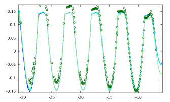
Figure 6: Comparison of the curvature scaling functions $f_{T}$ for the $\epsilon_{2}=0$ (black line), $\epsilon_{2}=10^{-2}$ (blue line), $\epsilon_{2}=0.1$ (cyan line), $\epsilon_{2}=0.5$ (light green line) and $\epsilon_{2}=0.75$ (dark green circles) families. Each $f_{T}$ is computed at the highest numerical resolution shown in Table 1. Here and in the following plots, the horizontal range is exactly the same in Figs. 1 and 2, and the distribution of data points is the same as indicated by circles there, but for clarity we no longer show those individual data points, except for $\epsilon_{2}=0.75$, where our computation at the highest resolution has gaps due to lack of computing time.

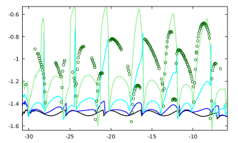
Figure 7: Comparison of the mass scaling function $f_{M}$ for the same values of $\epsilon_{2}$ as in Fig. 6: $\epsilon_{2}=0$ (black), $\epsilon_{2}=10^{-2}$ (blue), $\epsilon_{2}=0.1$ (cyan), $\epsilon_{2}=0.5$ (light green) and $\epsilon_{2}=0.75$ (dark green), at the same resolutions as there.

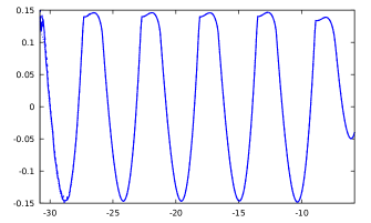
Figure 8: The curvature scaling function $f_{T}$ for $\epsilon_{2}=10^{-2}$ (blue), at three different angular resolutions: $\bar{N}_{y}=3$ (solid) $\bar{N}_{y}=5$ (dashed) and $\bar{N}_{y}=9$ (dotted), and $l_{\text{max}}=2,4,8$, respectively, all with $\Delta x=0.025$, $x_{0}=8.275$, $x_{\text{max}}=15$. The curves are indistinguishable, indicating that the errors from discretizing in $y$ are small.

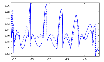
Figure 9: The mass scaling function $f_{M}$ for $\epsilon_{2}=10^{-2}$, at the same four resolutions as in Fig. 8. The differences in $f_{M}$ between resolutions are very large, compared to $f_{T}$ in Fig. 8.

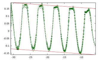
Figure 10: The curvature scaling function $f_{T}$ for $\epsilon_{2}=0.75$, at four different resolutions: $\bar{N}_{y}=17$, $\Delta x=0.005$ (our best resolution, circles), $\bar{N}_{y}=9$, $\Delta x=0.0025$, $x_{0}=24.5$ (dashed lines), and $\bar{N}_{y}=17$, $\Delta x=0.005$, $x_{0}=30$ (dotted), and $\tilde{N}_{y}=9$, $\Delta x=0.005$, $x_{0}=24$ (dot-dashed). The red straight lines represent a fit by eye to the local minima and maxima of $f_{T}$. They have slope $\delta\gamma=-0.0016$.

Figure 11: The mass scaling function $f_{M}$ for $\epsilon_{2}=0.75$, at the same four resolutions as in Fig. 10. The red straight lines have slope $\delta\gamma=-0.0016$, taken from the fit in Fig. 10. $f_{M}$ is both not periodic enough and too resolution-dependent for a meaningful fit to its average slope, but $\delta\gamma=-0.0016$ is consistent with the data.

IV.3 Self-similarity and evolution of the nonsphericity

We now test the hypothesis that there is a regime of small $\epsilon_{2}$ where near-critical time evolutions can be approximated by the spherical critical solution plus small perturbations, and attempt to find the limit of its validity.

We begin with the spherical part of the scalar field and metric. Under the assumption that ${\cal T}$ is still dominated by the derivatives of $\psi_{0}$, we adjust $u_{*}$ to make ${\cal T}$ as periodic as possible, and in particular with as many maxima and minima taking the same values, just as in the spherical case. We then find that $\psi_{0}(x,\tau)$, and $C(x,\tau)$, with the same fitted value of $u_{*}$, are essentially identical from $\epsilon_{2}=0$ through to $\epsilon_{2}=0.75$. See again the limit on a possible change of $\Delta$ of the critical solution documented above.

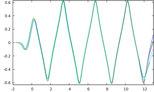
Figure 12: The scalar field at the centre, $\psi_{0}(0,\tau)$, at our best numerical resolution and best subcritical value of $p$, for each of $\epsilon_{2}=0$ (black), $10^{-4}$ (purple), $10^{-2}$ (blue), $0.1$ (cyan), $0.5$ (light-green) and $0.75$ (dark-green). The horizontal axis shows $\tau$ and the vertical axis $\psi$ at the centre.

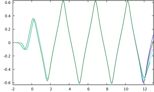
Figure 13: The same plot as in in Fig. 12, but a linear transformation applied to $\tau$ applied to $\epsilon_{2}=0.1$, $0.5$ and $0.75$ (but not the smaller values), in order to align the first and third full maxima. For this, $\tau$ is stretched by factors of $0.9995$, $1.0008$ and $1.0068$, respectively, as well as shifted.

We next address the hypothesis that the deviations from spherical symmetry are small and essentially linear.

To find the linear perturbations of a given spherical DSS critical solution $\phi_{*}$, one can separate the linearised equations by angular dependence $l$, and for each $l$ and dimensionless field $\phi$ make a mode ansatz

$$\delta\phi_{l}(\xi,\tau)=e^{\lambda\tau}\,\delta\tilde{\phi}_{l\lambda}(\xi,\tau),$$ (24)

with $\delta\tilde{\phi}_{l\lambda}$ defined to be periodic in $\tau$ with period $\Delta$, and regular at the centre and at the past lightcone. Here $\phi$ stands for any scale-invariant quantity, such as $\psi$ or ${\cal T}$. From this ansatz, the complex mode function $\delta\tilde{\phi}_{l\lambda}$ and corresponding complex Lyapunov exponent

$$\lambda:=\kappa+i\omega$$ (25)

are then determined as the eigenfunctions and eigenvalues of a (singular) linear boundary value problem JMMGundlach1999 . As the background solution and its perturbations are real (the complex mode ansatz is only for convenience), $\lambda$ and the corresponding $\delta\tilde{\phi}_{l\lambda}$ are either real or form complex conjugate pairs.

From these complex modes, one can construct the corresponding real perturbations as

$$\delta\phi_{l}(\xi,\tau) = {\rm Re}\left[Ae^{i\alpha}e^{(\kappa+i\omega)\tau}\,\delta\tilde{\phi}_{l\lambda}(\xi,\tau)\right]$$ (26)

$$= Ae^{\kappa\tau}[\cos(\omega\tau+\alpha)\,{\rm Re}\,\delta\tilde{\phi}_{l\lambda}(\xi,\tau)$$

$$-\sin(\omega\tau+\alpha)\,{\rm Im}\,\delta\tilde{\phi}_{l\lambda}(\xi,\tau)],$$

for arbitrary positive real amplitude $A$ and phase $0\leq\alpha<2\pi$. (Note this is slightly incorrect in Eq. (25) of Ref. Baumgarte2018 ). Unless $\omega$ is a rational multiple of $2\pi/\Delta$, the product $e^{-\kappa\tau}\delta\phi_{l}(\xi,\tau)$, while not growing or decaying, is nevertheless not periodic in $\tau$ but only quasiperiodic.

The perturbation modes of the spherical scalar field critical solution were found numerically in JMMGundlach1999 , using different similarity coordinates from the ones defined here. We can therefore compare the $\lambda$ with JMMGundlach1999 , but not directly the $\delta\tilde{\phi}_{l\lambda}(\tau,x)$. As expected for a critical solution, JMMGundlach1999 finds a single growing $l=0$ mode, with $\lambda$ and the corresponding mode function real. All other spherical modes, and all non-spherical modes, are complex and decay, that is, $\kappa<0$. The least damped (most slowly decaying) non-spherical mode was found to have $l=2$ angular dependence, with $\kappa\simeq-0.07/\Delta$ and $\omega/(2\pi)\simeq 0.3/\Delta$.

We expect that initial data which are almost spherical and fine-tuned to the threshold of collapse, but otherwise generic, evolve into something that can be approximated by the spherical critical solution plus a linear perturbation, and that the perturbation can be represented as sum of modes each with its own complex amplitude $Ae^{i\alpha}$ determined by the initial data.

During the intermediate range of $\tau$ where the solution is approximated by the critical solution plus small perturbations, we expect the least damped $l=2$ perturbation to dominate the $l=2$ component of the solution. The single-mode formula (26) should then approximately describe the $l=2$ component of near-critical evolutions in this regime. Moreover, its amplitude should be proportional to $\epsilon_{2}$, as the $l=2$ component of the initial data is proportional to $\epsilon_{2}$ to leading order.

In our initial data, the non-spherical part of $\psi$ is, to leading order in $\epsilon_{2}$, purely $l=2$, and so, going to quadratic order, we expect the initial data for the $l=4$ spherical harmonic component $\psi_{4}$ to be proportional to $\epsilon_{2}^{2}$. During the time evolution $\psi_{4}$ is sourced by terms that are linear in $f_{4}$ or quadratic in $f_{2}$ and $\psi_{2}$. $f_{4}$ is initially zero and then sourced by terms linear in $\psi_{4}$ and quadratic in $f_{2}$ and $\psi_{2}$. Perturbatively in $\epsilon_{2}$, we therefore expect all $l=2$ components to be proportional to $\epsilon_{2}e^{\kappa\tau}$, all $l=4$ components to be proportional to $\epsilon_{2}^{2}e^{2\kappa\tau}$, and so on for higher $l$.

To demonstrate the expected scaling with both $\tau$ and and $\epsilon_{2}$, in Fig. 14 we plot the maximum and minimum of $\epsilon_{2}^{-1}e^{-\kappa\tau}\psi_{2}(x,\tau)$ over $x$ in the range $0\leq x\leq 1$ against $\tau$, for different $\epsilon_{2}$, with our best subcritical $p$ at our best numerical resolution. The same is done in Fig. 15 for $f_{2}$. We find that $\epsilon_{2}^{-1}e^{-\kappa\tau}\psi_{2}$ is essentially the same at $\epsilon_{2}=10^{-4}$, $10^{-2}$ and $0.1$, and so is $\epsilon_{2}^{-1}e^{-\kappa\tau}f_{2}$. At $\epsilon_{2}=0.5$ and $0.75$, they are a bit larger (by a factor of $\sim 1.5$ at $\epsilon_{2}=0.75$), but still agree qualitatively feature by feature. In other words, $\psi_{2}$ and $f_{2}$ are almost linear up to $\epsilon_{2}=0.1$, and still approximately linear up to $0.75$.

In these plots, we have fitted $\kappa=-0.03$ by eye. Compare this with the value of $\kappa\simeq-0.07/\Delta\simeq-0.02$ determined in JMMGundlach1999 from a numerical construction of the eigenvalues of the operator evolving a linear perturbation from $\tau$ to $\tau+\Delta$. Neither is very accurate, but we believe that our fitted value is compatible with the theoretically expected one, but not with zero. In other words, we find that $\psi_{2}$ and $f_{2}$ decay as expected from the linear perturbation mode analysis, up to $\epsilon_{2}=0.75$.

Having established these scalings, we give the full surface plots for $\psi_{2}(x,\tau)$ and also $f_{2}(x,\tau)$, for $\epsilon_{2}=0.75$ in Figs. 16 and 17.

The $l=4$ modes of $\psi$ and $f$ in the best subcritical evolutions also seem to be quasiperiodic in $\tau$ and roughly independent of $\epsilon_{2}$ when rescaled with $\epsilon_{2}^{-2}e^{-2\kappa\tau}$. This is demonstrated in Figs. 18-21.

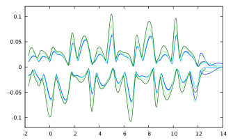
Figure 14: $\min_{x}$ and $\max_{x}$ of $\epsilon_{2}^{-1}e^{-\kappa\tau}\psi_{2}(x,\tau)$, plotted against $\tau$, for $\epsilon_{2}=10^{-4}$ (purple), $\epsilon_{2}=10^{-2}$ (blue), $\epsilon_{2}=0.1$ (cyan), $\epsilon_{2}=0.5$ (light green) and $\epsilon_{2}=0.75$ (dark green).

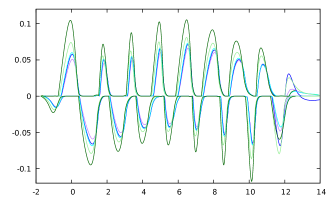
Figure 15: $\min_{x}$ and $\max_{x}$ of $\epsilon_{2}^{-1}e^{-\kappa\tau}f_{2}(x,\tau)$, plotted against $\tau$, otherwise as in Fig. 14.

Figure 16: Surface plot of the scaled non-spherical scalar field component $\epsilon_{2}^{-1}e^{-\kappa\tau}\psi_{2}(x,\tau)$, in the sub15 evolution of the $\epsilon_{2}=0.75$ family. Otherwise as described in Fig. 3. Note that the dark green curves in Fig. 14 are the projection of this surface plot in the $\xi$ direction.

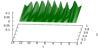
Figure 17: Surface plot of the scaled metric component $\epsilon_{2}^{-1}e^{-\kappa\tau}f_{2}(x,\tau)$ , otherwise as in Fig. 16.

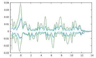
Figure 18: $\min_{x}$ and $\max_{x}$ of $\epsilon_{2}^{-2}e^{-2\kappa\tau}\psi_{4}(x,\tau)$, plotted against $\tau$, otherwise as in Fig. 14.

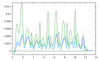
Figure 19: $\min_{x}$ and $\max_{x}$ of $\epsilon_{2}^{-2}e^{-2\kappa\tau}f_{4}(x,\tau)$, plotted against $\tau$, otherwise as in Fig. 14. Where the minimum is exactly zero, $f_{4}\geq 0$, with equality only at the origin.

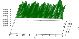
Figure 20: Surface plot of the scaled non-spherical scalar field component $\epsilon_{2}^{-2}e^{-2\kappa\tau}\psi_{4}(x,\tau)$ against the similarity coordinates $\xi$ and $\tau$, in the sub15 evolution of the $\epsilon_{2}=0.75$ family.

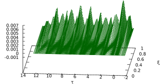
Figure 21: Surface plot of the scaled metric component $\epsilon_{2}^{-2}e^{-2\kappa\tau}f_{4}(x,\tau)$ , otherwise as in Fig. 20.

The mode frequency $\omega$ could in principle be obtained by a (discrete) Fourier transform of our data in $\tau$. We have not attempted this as the region where the background spherical solution is clearly DSS and the different perturbation amplitudes agree (after rescaling) is only $1\lesssim\tau\lesssim 9$, giving us only about two periods of the background solution. The discrete set of angular frequencies present in the Fourier transform with respect to $\tau$ of (26) is

$$\omega_{N}:=\omega+N{2\pi\over\Delta},\qquad N\in{\mathbb{Z}},$$ (27)

where the cited $\omega$ is the value for $N=0$, that is, the smallest positive frequency in the spectrum. Because of the symmetry $\psi(x,\tau+\Delta/2)=-\psi(x,\tau)$, $N$ takes odd values for the scalar field and even values for the metric. The spectrum obviously depends on the value of the parameter $\alpha$ in (26), but for a random $\alpha$, JMMGundlach1999 found that the peak of the spectrum was at $N=5$. The corresponding period in $\tau$ is

$$P_{N}:={2\pi\over|\omega_{N}|}={\Delta\over\left|N+{\omega\Delta\over 2\pi}\right|}\simeq{3.44\over|N+0.3|}.$$ (28)

If we count the peaks in Fig. 14, we find about 12 in the range $0\leq\tau\leq 12$, giving us a “pseudoperiod” of about 1, similar to $P_{3}\simeq 1.0$. If we count the peaks in Fig. 15, with find about 8 in the same range, giving us a pseudoperiod of about $2/3$, similar to $P_{5}\simeq 0.65$.

The numerical measurement of both $\kappa$ and $\omega$ would be improved in proportion to increasing the range of $\tau$ over which our fine-tuned numerical solutions approximate the critical solution. Going any further in this would require quadruple precision, not only so that $p$ can be represented to more significant figures, but more importantly so that round-off error during the numerical solution is suppressed better.

We note in passing that $\psi_{2}/x^{2}$, $f_{2}/x^{2}$ and $f_{4}/x^{4}$, which should be regular at $x=0$ in the continuum, are also numerically regular at $x=0$, but $\psi_{4}/x^{4}$ is not. (It is generally hard to enforce $f_{l}\sim r^{l}$ in any freely evolved variable, without explicitly taking out the factor $r^{l}$.)

IV.4 Comparison with the evolutions of Choptuik et al, Baumgarte, and Marouda et al

In order to compare the non-sphericity of our evolutions with those of Baumgarte2018 (and by implication also of Choptuiketal2003 for the same initial data), we note that Baumgarte has measured the difference in $\psi$ on outgoing null geodesics at $y=\pm 1$ and $y=0$ (poles and equator). Fig. 11 of Baumgarte2018 shows this $\delta\psi$ for $\epsilon_{2}=10^{-2}$ during the approximately self-similar phase, plotted against the similarity variables $\tau=-\ln(u_{*}-u)$ and $\xi_{\lambda}:=\lambda/(u_{*}-u)$, where $\lambda$ is the affine parameter, normalised to $\lambda=0$ and $d\lambda/dR=1$ at the origin, and $u_{*}$ is fitted as described above. This measure is gauge-invariant.

We note that for infinitesimal deviations from spherical symmmetry, and assuming the deviation only has an $l=2$ component,

$$\delta\psi(u,x) := \psi(u,x,\pm 1)-\psi(u,x,0)$$ (29)

$$= \left[P_{2}(\pm 1)-P_{2}(0)\right]\psi_{2}(u,x)$$ (30)

$$= {3\over 2}\psi_{2}(u,x),$$ (31)

where $\psi_{2}$ denotes the $l=2$ component of $\psi$. $\lambda$ along outgoing null geodesics is given by

$$\lambda(u,x,y)=\int_{0}^{x}G(u,x^{\prime},y)\,dx^{\prime}$$ (32)

The equivalent of Fig. 11 of Baumgarte2018 created from our data for $\epsilon_{2}=10^{-2}$ is Fig. 22. Note that in this plot we have not applied the factor of $e^{-\kappa\tau}$. (This makes little difference, as $\kappa$ is so small.) At small $\epsilon_{2}$ our solutions are a little more nonspherical than those of Baumgarte2018 , but recall that we set initial data on different slices.

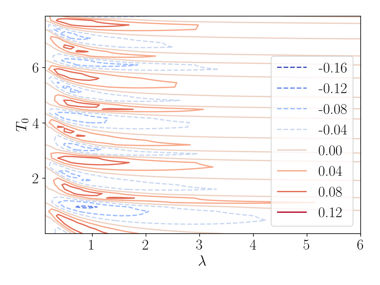
Figure 24: Contour plot of $\delta\psi/\epsilon^{2}$ against $\tau$ and $x_{\lambda}$ from the best subcritical $\epsilon^{2}=0.5$ evolution of Baumgarte Baumgarte2018 . This is the $\epsilon^{2}=0.5$ equivalent of Fig. 11 of Baumgarte2018 . $(\tau,x_{\lambda})$ are called $(T_{0},\lambda)$ in this plot. We have chosen a contour plot rather than a surface plot as this is clearer, given the coarse resolution of the available data.

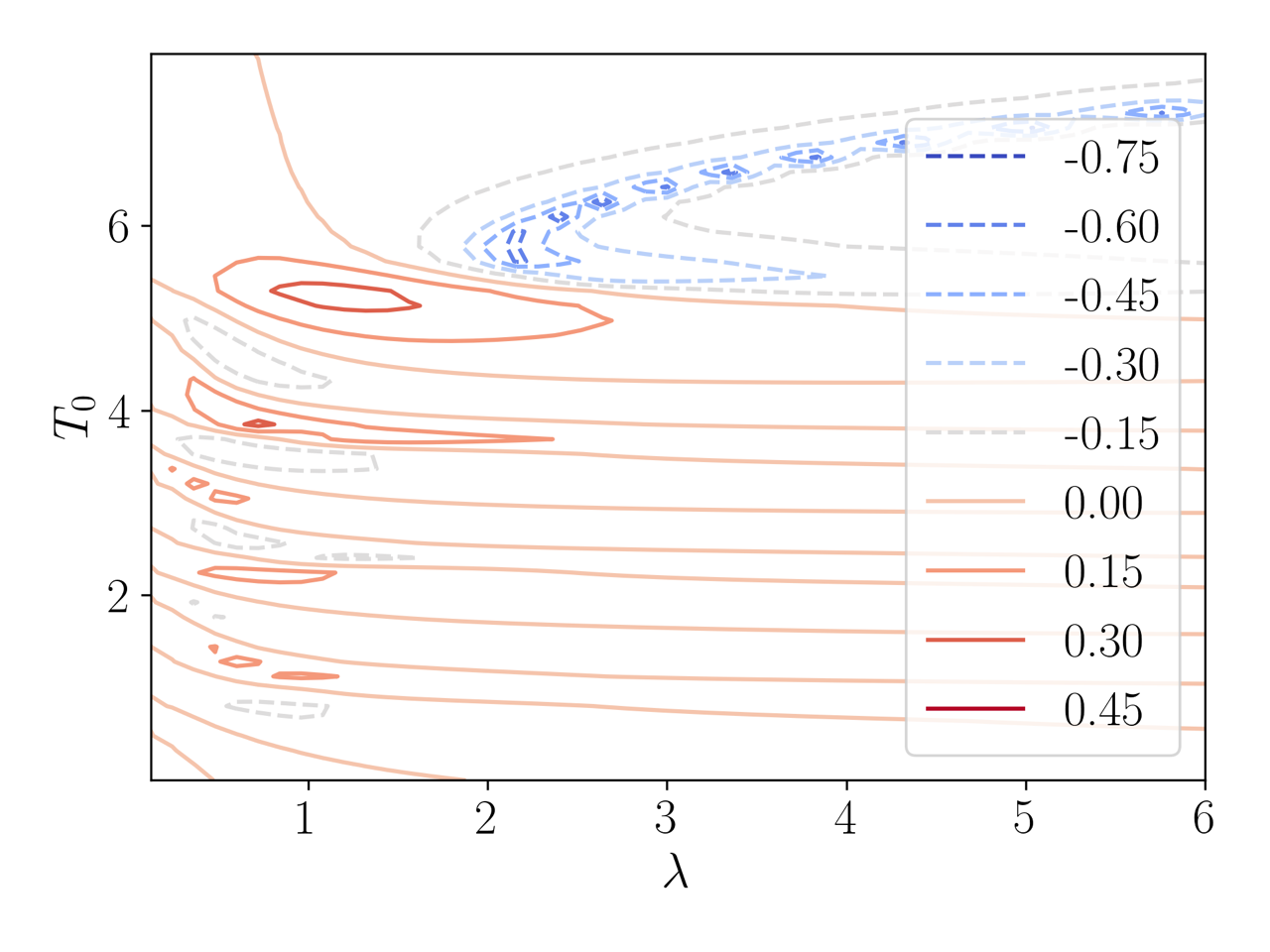
Figure 25: As in Fig. 24, but now for $\epsilon^{2}=0.75$. Note the sharp timelike feature in the range $6\leq T_{0}\leq 8$ that signals the end of approximate DSS (and, we expect, the formation of two centres of collapse).

Fig. 23 shows $\delta\psi$, approximated as $(3/2)\psi_{2}$ for our $\epsilon_{2}=0.75$. For comparison, Figs. 24 and 25 show plots of $\delta\psi$ created from the simulations of Baumgarte2018 for $\epsilon^{2}=0.5$ and $0.75$, respectively. This suggests that, during the approximately self-similar phase, our $\epsilon_{2}=0.75$ family is about as non-spherical as $\epsilon^{2}=0.5$ of Baumgarte2018 . In both families $\delta\psi$ does not grow noticeably. By contrast, Fig. 25 shows clear growth of $\delta\psi$ with $\tau$ for $\epsilon^{2}=0.75$ and an end to the perturbative regime around $\tau=6$.

Table 2 compares the black hole threshold in selected families taken from Choptuiketal2003 , Baumgarte2018 , Maroudaetal2024 and the present paper. Families that should be directly comparable are grouped together. For comparison have translated $\delta\psi/\epsilon^{2}$ and $\psi_{2}$ into $\delta\psi$ (by multiplying by $\epsilon^{2}$ and $3/2$, respectively). The values for $\max|\delta\psi|$ from the null code and that of Baumgarte2018 are read off from plots shown in the present paper. The values for $\epsilon^{2}=0$ and $\epsilon^{2}=2/3$ of Choptuiketal2003 are read off from Figs. 6 and 7 of that paper, respectively. In the spherically symmetric case we include $\max|\delta\psi|$ as an estimate of the numerical error generated by evolving a spherically symmetric solution in cylindrical coordinates. Finally, the values for families II, III and IV of Maroudaetal2024 are read off from plots communicated by the authors.

A range given for $\max|\delta\psi|$ means that its value increases noticeably from the beginning to the end of the phase where the spherical part of the solution is approximated by the Choptuik solution. A single value implies that the amplitude does not grow noticeably. (This is estimated by eye, as the perturbations are only quasiperiodic.)

By contrast, the ranges given for $\delta\gamma$ and $\delta\Delta$ express uncertainty: in the four papers, up to three different methods have been used to estimate $\Delta$ (but only one for $\gamma$). Independently, one can use either the numerical values of $\gamma$ and $\Delta$ obtained in spherical symmetry in each paper, or their known exact values as reference values. We cite here the largest and smallest of these (up to six) possible differences, in order to indicate a plausible interval for $\delta\gamma$ and $\delta\Delta$ for each family. We do not include the fitting errors given in Choptuiketal2003 ; Maroudaetal2024 , as these appear to be smaller than the systematic errors suggested by the intervals just mentioned.

We have attempted to order the families across papers, taking as our first ordering criterion the bifurcation (yes or no) of the critical solution, as our second criterion $\max|\delta\psi|$ (where we have data), and otherwise $\delta\gamma$ and $\delta\Delta$.

The fact that we are able to order the families of initial data consistently (within the estimated plausible ranges) is one of the main physics results of this paper. It supports the hypothesis that all near-critical evolutions go through a phase where the solution can be approximated by the Choptuik solution plus the growing spherical mode and the least damped $l=2$ mode. Large nonsphericity seems to change the values of $\Delta$ and $\gamma$, as well as the decay rate $\kappa$ of the $l=2$ mode, such that for non-sphericities of $\max|\delta\psi|\gtrsim 0.1$ it actually grows. (Compare this with $\max|\psi_{*}|\simeq 0.6$ for the critical solution.)

The exception from this consistent picture are the values of $\delta\gamma$ and $\delta\Delta$ obtained in this paper. Up to our $\epsilon_{2}=0.5$ family, these are zero within our estimated numerical errors. For our $\epsilon_{2}=0.75$ family, we have a signifant but small change of $\delta\Delta\sim 10^{-3}$ (but not of $\delta\gamma$), but this is still an order of magnitude smaller than $\delta\Delta$ observed in the other three papers at what we take to be comparable non-sphericity. For lack of a better explanation we suspect that this is due to some systematic numerical error, more likely in the null code than the other three codes.

Paper	Family	$\max|\delta\psi|$	$\delta\gamma$	$\delta\Delta$	Bif.
Choptuik+	$\epsilon^{2}=0$	$0_{(i)}...0.05_{(f)}$	$0.008_{(e)}$	$0_{(1,e)}...0.05_{(2,e)}$	no
Baumgarte	$\epsilon^{2}=0$	0	$0_{(e)}$	$0.02_{(3,e)}...0.03_{(1,e)}$	no
Marouda+	I	—	$-0.004_{(e)}$	$-0.02_{(3,e)}...0.01_{(1,e)}$	no
this paper	$\epsilon_{2}=0$	$0$	$0_{(e)}$	$0_{(e)}$	no
Baumgarte	$\epsilon^{2}=10^{-2}$	$0.005$	$0_{(e)}$	$-0.02_{(3,n12)}...0.03_{(1,e)}$	no
this paper	$\epsilon_{2}=10^{-2}$	$0.008$	$<10^{-3}$	$<10^{-3}$	no
Marouda+	II	$0.02$	$-0.002_{(e)}...0.002_{(n)}$	$-0.07_{(3,e)}...0.03_{(2,e)}$	no
Marouda+	III	$0.06$	$-0.010_{(e)}...-0.006_{(n)}$	$-0.12_{(3,e)}...-0.05_{(2,e)}$	no
this paper	$\epsilon_{2}=0.5$	$0.07$	$<10^{-3}$	$<10^{-3}$	no
Choptuik+	$\epsilon^{2}=0.5$	—	$-0.007_{(n)}...0.001_{(e)}$	$-0.12_{(1,n2)}...-0.05_{(2,e)}$	no
Baumgarte	$\epsilon^{2}=0.5$	$0.08$	$-0.005_{(e)}$	$-0.12_{(3,n1)}...-0.05_{(1,e)}$	no
Choptuik+	$\epsilon^{2}=2/3$	$0.06_{(i)}...0.12_{(f)}$	$-0.036_{(n)}...-0.028_{(e)}$	$-0.41_{(2,n2)}-0.31_{(1,e)}$	no
this paper	$\epsilon_{2}=0.75$	$0.09$	$-0.0016_{(e)}$	$-0.023$	no
Marouda+	IV	$0.1_{(i)}...0.2_{(f)}$	$-0.045_{(e)}...-0.041_{(n)}$	$-0.49_{(1,e)}...-0.35_{(2,e)}$	yes
Choptuik+	$\epsilon^{2}=0.75$	—	$-0.069_{(e)}...-0.061_{(n)}$	$-0.62_{(1,n2)}...-0.41_{(2,e)}$	yes
Baumgarte	$\epsilon^{2}=0.75$	$0.11_{(i)}...0.34_{(f)}$	$-0.068_{(e)}$	$-0.72_{(3,n1)}...-0.57_{(1,e)}$	yes
Choptuik+	$\epsilon^{2}=5/6$	—	$-0.102_{(n)}...-0.094_{(e)}$	$-2.49_{(2,n2)}...-1.44_{(1,e)}$	yes

Table 2: Comparison of families of initial data near the black hole threshold, combining data from our evolutions with those of Choptuiketal2003 , Baumgarte2018 and Maroudaetal2024 . Families corresponding to the same initial data have been grouped together. A dash means no data are available. A range given for $\max|\delta\psi|$ means that its value increases noticeably during the phase where the spherical part of the solution is approximated by the Choptuik solution. By contrast, the ranges given for $\delta\gamma$ and $\delta\Delta$ express uncertainty, see the main text for details. Footnotes: (e) relative to exact values $\Delta\simeq 0.374$ and $\Delta\simeq 3.44$ in spherical symmetry; (n) relative to numerical value obtained in spherical symmetry; (i) initial and (f) final value in the approximately Choptuik phase; (1) first, (2) second and (3) third method of determining $\Delta$; (3,n1), for example means, the numerical value of $\Delta$ in a non-spherical evolution obtained by the third method, relative to the numerical value determined by the first method in spherical symmetry.

IV.5 Numerical problems at larger non-sphericity

We have already mentioned that to complete the bisection in $p$ for $\epsilon_{2}=0.75$ at our highest resolution $\bar{N}_{y}=17$, $\Delta x=0.025$, we had to lower our heuristic diagnostic of collapse to $C\geq 0.8$.

We have tried to bisect at $\epsilon_{2}=0.79$, with $\bar{N}_{y}=17$, $\Delta x=0.05$, and again using $C\geq 0.8$ as the collapse diagnostic, starting again with the initial bracket $0.2<p_{*}<0.3$. Already at the third bisection step, the code stops because $B$ becomes very large at the boundary, and so the time step becomes very small. On closer inspection, $B$ becomes very irregular at late times at the outermost few points, and very much larger at the outermost grid point than anywhere else. This cannot be a boundary instability in the usual sense because the outer boundary is treated exactly like an ordinary grid point. Hence the instability must be one that grows much faster at larger $x$, and so most rapidly at the outer boundary.

We believe what is at fault here is a combination of two problems we have already mentioned. One is that in our gauge, we evaluate $\min_{y}\Xi R(u,x,y)$, and this means that the $B_{,x}$ becomes discontinuous. This lack of smoothness then propagates to the other variables. A separate problem is that $R_{,x}$ becomes small as outgoing light cones are trying to recollapse, while lsB gauge (or any gauge which solves the Raychaudhuri equation along null generators for $G$ rather than for $R$) requires $R_{,x}>0$. We believe this would still give rise to very large values of $B$ even if we found a better gauge within the lsB family that avoided the unsmoothness.

V Conclusions

This work was born out of an attempt to generalise the method of Garfinkle Garfinkle1995 for simulating critical collapse without the need for adaptive mesh refinement beyond spherical symmetry. We have demonstrated that this is possible, in the example of axisymmetric scalar field critical collapse.

We have attempted to duplicate previous physics results as well. Recall that the collapse simulations of Baumgarte (in spherical polar coordinates) Baumgarte2018 seemed to have reconciled the linear perturbation results of Martín-García and Gundlach JMMGundlach1999 with the collapse simulations of Choptuik et al Choptuiketal2003 (in cylindrical coordinates): small deviations from spherical symmetry decay when one fine-tunes to the threshold of collapse, while large perturbations grow and lead to the formation of two centres of collapse. This conclusion is also supported by the more recent evolutions of Maroudaetal2024 and (less quantitatively) of Reid2023 .

Specifically, Baumgarte2018 and Choptuiketal2003 find that non-sphericities decay for values of their non-sphericity parameter $\epsilon^{2}\leq 0.5$, and Choptuiketal2003 still find this at $\epsilon^{2}=2/3$. Both Baumgarte2018 and Choptuiketal2003 find a bifurcation for $\epsilon^{2}=0.75$, and Choptuiketal2003 also at $\epsilon^{2}=5/6$. (We note that Maroudaetal2024 also observe bifurcation in their most non-spherical data for the complex scalar field). Choptuiketal2003 , Baumgarte2018 and Maroudaetal2024 also found that $\Delta$ and $\gamma$ (measured before any bifurcation occurs) decrease with increasing $\epsilon_{2}$, see Table 1 for representative numerical values.

By contrast, we have found that even in the evolution of our $\epsilon_{2}=0.75$ family of data perturbation theory is a good model for the non-sphericity. In particular, the echoing period and critical exponent remain at $\Delta\simeq 3.44$ and $\gamma\simeq 0.374$, their values in spherical symmetry, and the $l=2$ non-spherical components of all fields decay at roughly the rate predicted for linear perturbations in JMMGundlach1999 . We also find that the amplitude of the $l=2$ field components is almost linear in $\epsilon_{2}$ for values between $10^{-4}$ and $0.75$, enhanced only by a factor $\sim 1.5$ at $\epsilon_{2}=0.75$. Similarly, the $l=4$ non-sphericity scales with $(\epsilon_{2})^{2}$, as one would expect from perturbation theory to quadratic order, given that $l=4$ is absent in the initial data to linear order in $\epsilon_{2}$, and that JMMGundlach1999 predicts $l=4$ to decay much more rapidly than $l=2$.

However, we cannot evolve the same family of initial data as Baumgarte2018 and Choptuiketal2003 , because we set data on an outgoing null cone. We have compared a gauge-invariant measure of the non-sphericity of the scalar field, in the phase where a near-critical evolution is approximately self-similar, with the same measure for the evolutions of Baumgarte2018 , and find that this comparable between our $\epsilon_{2}=0.5$ and $\epsilon^{2}=0.75$ of Baumgarte2018 (and by implication of Choptuiketal2003 ). If we compare our $\epsilon_{2}=0.5$ with $\epsilon^{2}=0.75$ of Baumgarte2018 ; Choptuiketal2003 , a mild tension remains, as these authors claim that $\Delta\simeq 3.44$ is reduced by $\sim 0.08$ and $\gamma\simeq 0.374$ by $\sim 0.007$, whereas we see much smaller reductions. This could potentially still be explained by numerical error.

In order to accurately measure the critical exponent $\gamma$, we have fitted not only the power laws with exponent $\gamma$, but also the small periodic fine-structure superimposed on them. This has only been done in spherical symmetry before. Our fine-structure of the curvature scaling laws (on the subcritical side) agrees well with published results in spherical symmetry, but our fine structure of the mass scaling law does not. The reason may be that our collapse criterion is not the first appearance of a trapped surface (in a given time slicing) but the first appearance of a coordinate 2-surface ${\cal S}_{u,x}$ with Hawking compactness above a threshold value, and we evaluate the Hawking mass of that surface.

We believe this is the first simulation of gravitational collapse beyond spherical symmetry in null coordinates. (The paper Siebeletal2003 investigates axisymmetric supernova core collapse, but not black hole formation.) We have applied our methods to the challenging problem of axisymmetric scalar field critical collapse, and at moderate non-sphericity have been able to fine-tune our initial data to the black-hole threshold to machine precision, without the need for mesh refinement.

We have not yet been able to simulate critical collapse for large enough non-sphericity to fully duplicate the results of Baumgarte2018 ; Choptuiketal2003 ; Maroudaetal2024 : at large non-sphericity, our evolutions stop before we can classify them as either forming a black hole or dispersing. The proximate cause for this is that the divergence of the null generators of our coordinate lightcones is trying to become negative at some points on our last null cone, but the generalised Bondi coordinates we use break down if this happens. Therefore, the next step will be to change to a generalised affine radial coordinate. This will then allow us to investigate if our null cones themselves remain regular in critical collapse, or form caustics.

Appendix A Family-dependent parameters in the fine structure of the scaling laws

In this Appendix, we show that the parameters $A$ and $B$ in Eqs. (15) and (16) are family-dependent, and independent of each other.

Focus first on the late-time evolution of the exactly-critical member of a given 1-parameter family of initial data. If we fix a (family-independent) small length scale $L$, then we can, for example, measure the phase of the scalar field $\phi$ at the centre when the Ricci scalar at the centre takes exactly the value $L^{-2}$. This is equivalent to our $A$.

On the other hand, to derive the scaling laws we use the fact that in near-critical evolutions the amplitude of the growing perturbation is, to leading order, proportional to $(p-p_{*})e^{\lambda_{0}\tau}$. The constant of proportionality must again be family-dependent, already for the trivial reason that $p$ can have any dimension. Its logarithm is our $B$.

Note that for perfectly-critical initial data the growing perturbation of the critical solution is by construction absent, while the scaling laws rely on the amplitude of the growing mode. Hence the family-dependent constants $A$ and $B$ are independent of each other.

Appendix B Convergence tests in the strong subcritical regime

For convergence testing we choose our $\epsilon_{2}=0.75$ initial data with the two amplitudes that we have also used as an initial bracket of the black hole threshold, namely $p=0.2$ (subcritical) and $p=0.3$ (supercritical). We use the grid parameters $x_{\text{max}}=50$ and $x_{0}=33$ throughout, which we also used in our near-critical evolutions.

For $p=0.2$ gravity is strong but not close to collapse, with a maximum Hawking compactness of $\bar{C}\simeq 0.08$ in the initial data, and reaching $\bar{C}\simeq 0.2$ during the evolution (compared to $\bar{C}\simeq 0.6$ in the critical solution and $\bar{C}=1$ on a black-hole horizon). We run to $u=6$, when the solution has largely dispersed, with $\bar{C}<0.01$, but the numerical domain has contracted from $R_{\text{max}}=25$ at the initial time only to $R_{\text{max}}\simeq 14$, thus avoiding very small timesteps.

The evolutions with $p=0.3$ start from $\bar{C}\simeq 0.18$ and reach our heuristic collapse criterion $\bar{C}=0.8$ at $u\simeq 3.9$, at which point we stop the evolution.

Both $p=0.2$ and $p=0.3$ are far enough from $p_{*}\simeq 0.25$ that it remains meaningful to compare numerical solutions with different resolutions at the same coordinate time $u$ and amplitude $p$, as $|p_{*}-p|\simeq 0.05$ is then much larger than the variation of $p_{*}$ with different numerical parameters. By contrast, in the critical regime we would need to compare different resolutions at the same (small) $p/p_{*}-1$, with $p_{*}$ resolution-dependent, and plot them against the similarity-adapted coordinates $(\tau,\xi)$, which also depend sensitively on numerical parameters through the fitted value of $u_{*}$.

We output all fields as $l$-components (rather than against $y$) to make comparisons at different $\bar{N}_{y}$ and $l_{\text{max}}$ simpler. We have tested for self-convergence to second order in $\Delta x$ and in $l_{\text{max}}$, see Paper I for details of how the errors presented here are defined.

We have evolved at two intersecting families of resolutions: at $\Delta x=\{0.1,{\bf 0.05},0.025,0.0125\}$ with fixed angular resolution $\bar{N}_{y}=17$, $l_{\text{max}}=16$; and at $\bar{N}_{y}=\{9,13,{\bf 17},25,33,49,65\}$, $l_{\text{max}}=\bar{N}_{y}-1$, with fixed radial resolution $\Delta x=0.05$. Their intersection is our baseline solution, chosen because the discretisation errors in $x$ and $y$ are roughly similar. Note that our adaptive timestep $\Delta u$ is approximately proportional to $\Delta x$ and approximately independent of angular resolution.

We find a large and non-converging error at small $u$ and $x$, in all $\psi_{l}$ with $l>2$. We believe this is due to the fact that our initial data (11-12) is not actually single-valued at the origin. The non-convergent error disappears quickly, and we believe this is because the boundary conditions at the centre force the solution to become single-valued.

At all other $(u,x)$ we find the expected second-order convergence in $\Delta x$. For a spectral method acting on a smooth solution, we would expect approximately exponential convergence, but in fact the discretisation error in $y$ decreases with resolution only as $l_{\text{max}}^{-2}$. Second-order convergence in the $L^{2}$ norm with $\Delta x$ and $1/l_{\text{max}}$ is demonstrated for $\psi_{0}$ in Fig. 26, for $\psi_{4}$ in Fig. 27, and for $\bar{C}$ in Fig. 28. The convergence is actually pointwise. The global maximal errors $\max_{u}||{\cal E}_{x}||_{L^{2}}$ and $\max_{u}||{\cal E}_{y}||_{L^{2}}$ for the dispersing are shown in Table 4. Given second-order convergence, we can accurately estimate the error at all higher resolutions by scaling these numbers by factors $(\Delta x/0.05)^{2}$ and $(l_{\text{max}}/16)^{-2}$, respectively.

The computation of the diagnostic $\bar{C}$ in the collapsing solution seems to be particularly challenging. Here we see clear second-order convergence, even at early times, only for $\bar{N}_{y}\geq 25$, see the lower plot in Fig. 28.

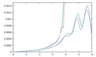
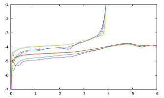
Figure 26: Upper plot: $L^{2}$ norm of the discretisation error in $x$ of the spherical scalar field component $\psi_{0}(u,x)$, shown against $u$, for $\Delta x=\{0.1,0.05,0.25\}$ (purple, green, blue), scaled to the baseline resolution $\Delta x=0.05$ by assuming that the error scales as $\Delta x^{2}$. The angular resolution is fixed at $\bar{N}_{y}=17$, $l_{\text{max}}=16$. The lower group of three curves is for the $p=0.2$ evolutions, and the upper group for the $p=0.3$ evolutions. Lower plot: $\log_{10}$ of the $L^{2}$ norm of the discretisation error in $y$ for $\bar{N}_{y}=\{9,13,17,25,33,49\}$ (purple, green, blue, orange, yellow, red) scaled to the baseline resolution $\bar{N}_{y}=17$, $l_{\text{max}}=16$ assuming that the error scales as $l_{\text{max}}^{-2}$. The radial resolution is fixed at $\Delta x=0.05$.

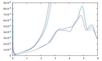
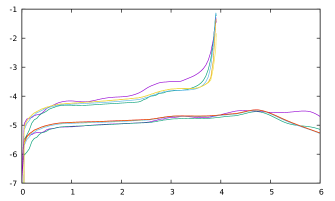
Figure 27: As in Fig. 26, but now for $\psi_{4}$. The large spike at $u=0$ (not fully shown, and not convergent) is a signal of the irregularity of our initial conditions. All $\psi_{l}$ with $l>2$ have this problem.

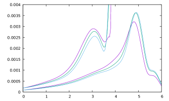
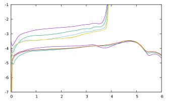
Figure 28: As in Fig. 26, but now for $\bar{C}$.

$\epsilon_{2}$	$\Delta x$	$\bar{N}_{y}$	$l_{\text{max}}$	$x_{0}$	$x_{\text{max}}$
0.5	0.025	9/17	8/16	29	30
0.6	0.025	9/17	8/16	39	40
0.7	0.05	17	16	99	100
0.75	0.05	17	16	149	150

Table 3: Successful initial bracketings of the collapse threshold with the analytic initial data (38). In each case, $p=0.2$ disperses and $p=0.3$ collapses. $x_{\text{max}}$ needs to be this large only for the collapsing solutions. $x_{\text{max}}$ is twice as large as for the non-analytic data (10) for $\epsilon_{2}=0.5$, and three times as large for $\epsilon_{2}=0.75$. $x_{0}$ has not yet been fine-tuned for bisection to the black hole threshold. We have used $\bar{C}\geq 0.8$ as the collapse threshold and $\bar{C}\leq 0.05$ as the dispersion threshold.

non-analytic	$\psi_{0}$	$\psi_{4}$	$\bar{C}$
$\max_{u}||{\cal E}_{x}||_{L^{2}}$	$1.3\cdot 10^{-3}$	$8\cdot 10^{-5}$	$3.5\cdot 10^{-3}$
$\max_{u}||{\cal E}_{y}||_{L^{2}}$	$1.7\cdot 10^{-4}$	$3\cdot 10^{-5}$	$3\cdot 10^{-4}$
analytic	$\psi_{0}$	$\psi_{4}$	$\bar{C}$
$\max_{u}||{\cal E}_{x}||_{L^{2}}$	$2\cdot 10^{-3}$	$5\cdot 10^{-4}$	$7\cdot 10^{-3}$
$\max_{u}||{\cal E}_{y}||_{L^{2}}$	$1.2\cdot 10^{-2}$	$4\cdot 10^{-3}$	$2\cdot 10^{-2}$

Table 4: Table of the maximum in $u$ of the $L^{2}$ norm in $x$ and $y$ of the discretisation errors in $x$ and $y$, in the three variables $\psi_{0}$, $\psi_{0}$ and $\bar{C}$, in the $p=0.2$ (dispersing) solution, at the baseline resolution $\Delta x=0.0.5$, $\bar{N}_{y}=17$, $l_{\text{max}}=16$. Top: non-analytic data. Bottom: analytic data.

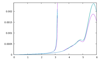
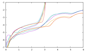
Figure 29: Error in $\psi_{0}$ as in Fig. 26, but now for the analytic initial data (38) with $\epsilon_{2}=0.75$, and with errors in $y$ now scaled by $\exp[-\kappa(l_{\text{max}}-16)]$ with $\kappa\simeq 0.280$ for $l_{\text{max}}=8,12,16$ and $\kappa\simeq 0.085$ for $l_{\text{max}}=24,32,48$.

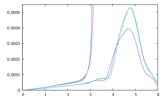
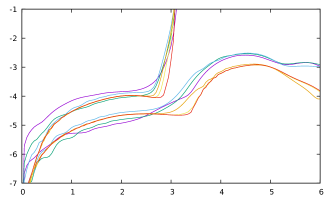
Figure 30: As in Fig. 29, but now for $\psi_{4}$.

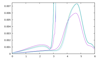
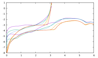
Figure 31: As in Fig. 29, but now for $\bar{C}$.

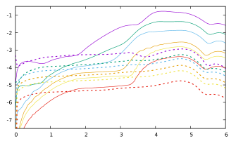
Figure 32: Direct comparison of the unscaled discretization errors in $y$ for the non-analytic (dashed lines) and analytic (solid lines) $\epsilon_{2}=0.75$, $p=0.2$ data. As before $\bar{N}_{y}=\{9,13,17,25,33,49\}$ are shown in purple, green, blue, orange, yellow, red, and we estimate the error by subtracting the $\bar{N}_{y}=65$ evolutions.

Appendix C Convergence tests with initial data that are regular at the origin

To check the effect of our non-analytic original choice of initial data (where $\psi$ is not single-valued at the origin) on convergence, we have created a second family of initial data that are analytic.

We computed the exact solution $\phi_{(2k)}(t,r,y)$ of the flat spacetime scalar wave equation with Cauchy data

$$\phi_{(2k)}(0,r,y) = e^{-r^{2}}(-ry)^{2k},$$ (33)

$$\phi_{(2k),t}(0,r,y) = 0,$$ (34)

for $k=0,1,\dots 5$. (Recall that $y:=-\cos\theta$. We have set the width of the Gaussian to $d=1$ to fix an overall scale). These can be found as linear combinations of the generalised d’Alembert solutions $\phi_{l}(t,r)P_{l}(y)$ constructed in Paper I, for even $l$ up to $2k$, each with an ansatz for the free function $\chi_{l}(r)$ of that is $\exp(-r^{2})$ times an odd polynomial in $r$ of order $l+1$.

We then use the $\phi_{(2k)}(t,r,y)$ as building blocks to construct the solution with initial data

$$\bar{\phi}(0,r,y) = pe^{-r^{2}}\sum_{k=0}^{5}{(\epsilon_{2}r^{2}y^{2})^{k}\over k!}$$ (35)

$$= p\,e^{-{r^{2}(1-\epsilon_{2}y^{2})}}+O(\epsilon^{6}r^{12}y^{12}),$$ (36)

$$\phi_{,t}(0,r,y) = 0.$$ (37)

We then read off the desired null data at $u=0$ from the full solution as

$$\psi(0,r,y)=\bar{\phi}(r,r,y).$$ (38)

We were able to compute up to $k=6$ in Mathematica, and the error in the Taylor series is then below machine precision. However, in contrast to the $k\leq 5$ terms, the $k=6$ term would need to be approximated near $r=0$ to avoid large roundoff error when evaluating the exact expression numerically in the code, so we settle for the above truncation at $k=5$.

Table 3 shows successful initial brackets of the black hole threshold with the analytic data. We have not bisected the analytic data to the black hole threshold.

For convergence testing, we have evolved $\epsilon_{2}=0.75$, $p=0.2$ and $p=0.3$, at the same two intersecting families of resolution as for our non-analytic data. We again see second-order convergence in $\Delta x$. Power-law convergence in $l_{\text{max}}$ is no longer a good fit. A better fit is exponentional convergence in $l_{\text{max}}$ with a break in the exponent, namely $\exp[-\kappa(l_{\text{max}}-16)]$ with $\kappa\simeq 0.280$ for $l_{\text{max}}=8,12,16$ and $\kappa\simeq 0.085$ for $l_{\text{max}}=24,32,48$.

Numerical values for the errors at the baseline resolution are shown in Table 4, and $L^{2}$ norms over $x$ of the errors in $\psi_{0}$, $\psi_{4}$ and $\bar{C}$ are shown in Figs. 29, 30 and 31. For completeness, we show the unscaled errors in $y$, for the variable $\bar{C}$, and for both the analytic and non-analytic $\epsilon_{2}=0.75$, $p=0.2$ data in Fig. 32.

References

- (1) C. Gundlach, D. Hilditch and T. W. Baumgarte, Simulations of gravitational collapse in null coordinates I: Formulation and weak-field tests in generalised Bondi gauges, arXiv:2404.15105.
- (2) C. Gundlach and J. M. Martín-García, Critical phenomena in gravitational collapse, Living Rev. Relativ. 7, 05 (2007).
- (3) J. M. Martín-García and C. Gundlach, All nonspherical perturbations of the Choptuik spacetime decay, Phys. Rev. D 59, 064031 (1999).
- (4) M. W. Choptuik, E. W. Hirschmann, S. L. Liebling and F. W. Pretorius, Critical collapse of the massless scalar field in axisymmetry, Phys. Rev. D 68, 044077 (2003).
- (5) T. W. Baumgarte, Aspherical deformations of the Choptuik spacetime, Phys. Rev. D 98, 084012 (2018).
- (6) M. W. Choptuik, Universality and scaling in gravitational collapse of a massless scalar field, Phys. Rev. Lett. 10, 1103 (1993).
- (7) J. M. Martín-García and C. Gundlach, Global structure of Choptuik’s critical solution in scalar field collapse, Phys. Rev. D 68, 024011 (2003).
- (8) J. Healy and P. Laguna, Critical collapse of scalar fields beyond axisymmetry, Gen. Relativ. Gravit. 46, 1722 (2014).
- (9) N. Deppe, L. E. Kidder, M. A. Scheel and S. A. Teukolsky, Critical behavior in 3D gravitational collapse of massless scalar fields, Phys. Rev. D 99, 024018 (2019).
- (10) K. Clough and E. A. Lim, Critical Phenomena in Non-spherically Symmetric Scalar Bubble Collapse, unpublished, https://arxiv.org/abs/1602.02568.
- (11) G. D. Reid and M. W. Choptuik, Universality in the critical collapse of the Einstein-Maxwell system, Phys. Rev. D 108, 104021, (2023).
- (12) K. Marouda, D. Cors, H. R. Rüter, F. Atteneder and D. Hilditch, Twist-free axisymmetric critical collapse of a complex scalar field, arXiv:2402.06724
- (13) D. Garfinkle, Choptuik scaling in null coordinates, Phys. Rev. D 51, 5558 (1995).
- (14) C. Gundlach, T. W. Baumgarte and D. Hilditch, Critical phenomena in gravitational collapse with two competing massless matter fields, Phys. Rev. D 100, 104010 (2019).
- (15) O. Rinne, Type II critical collapse on a single fixed grid: a gauge-driven ingoing boundary method, Gen. Relativ. Gravit. 52, 117 (2020).
- (16) B. Porto-Veronese and C. Gundlach, Critical phenomena in gravitational collapse with competing scalar field and gravitational waves in 4+1 dimensions, Phys. Rev. D 106, 104044 (2022).
- (17) C. Gundlach, Understanding critical collapse of a scalar field, Phys. Rev. D 55, 695 (1996).
- (18) M. Pürrer, S. Husa and P. C. Aichelburg, News from critical collapse: Bondi mass, tails, and quasinormal modes, Phys. Rev. D 71, 104005 (2005).
- (19) J. A. Crespo, H. P. de Oliveira and J. Winicour, The affine-null formulation of the gravitational equations: spherical case, Phys. Rev. D 100, 104017 (2019).
- (20) D. Garfinkle and G. C. Duncan, Scaling of curvature in subcritical gravitational collapse, Phys. Rev. D 58, 064024 (1998).
- (21) D. Cors, S. Renkhoff, H. R. Rüter, D. Hilditch and B. Brügmann, Formulation improvements for critical collapse simulations, Phys. Rev. D 108, 124021, (2023).
- (22) F. Siebel, J. A. Font, E. Müller and P. Papadopoulos, Axisymmetric core collapse simulations using characteristic numerical relativity, Phys. Rev. D 67, 124018 (2003).