Isolated regions of a link projection
Abstract
A set of regions of a link projection is said to be isolated if any pair of regions in the set share no crossings. The isolate-region number of a link projection is the maximum value of the cardinality of an isolated set of regions of the link projection. In this paper, all the link projections of isolate-region number one are determined. Also, estimations for welded unknotting number and combinatorial way to find the isolate-region number are discussed, and a formula of the generating function of isolated-region sets is given for the standard projections of -torus links.
1 Introduction
A knot is an embedding of a circle in and a link is an embedding of some circles in . We assume a knot to be a link with one component. A link projection is a regular projection of a link on such that any intersection is a double point where two arcs intersect transversely. We call such an intersection a crossing. We call each connected part of divided by a link projection a region. It is well known that the number of regions is greater than the number of crossings by two111See, for example, [2]. for each link projection.
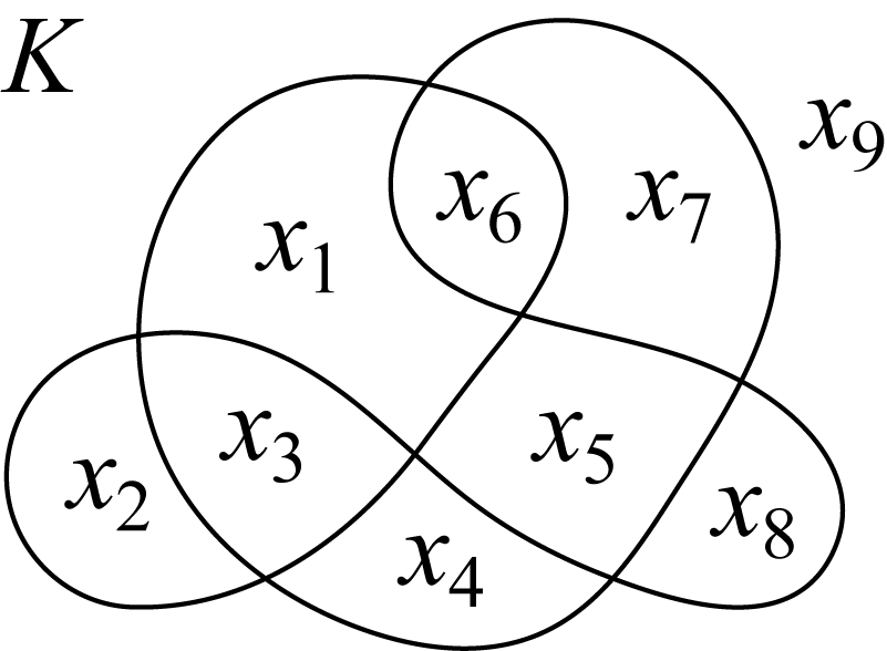
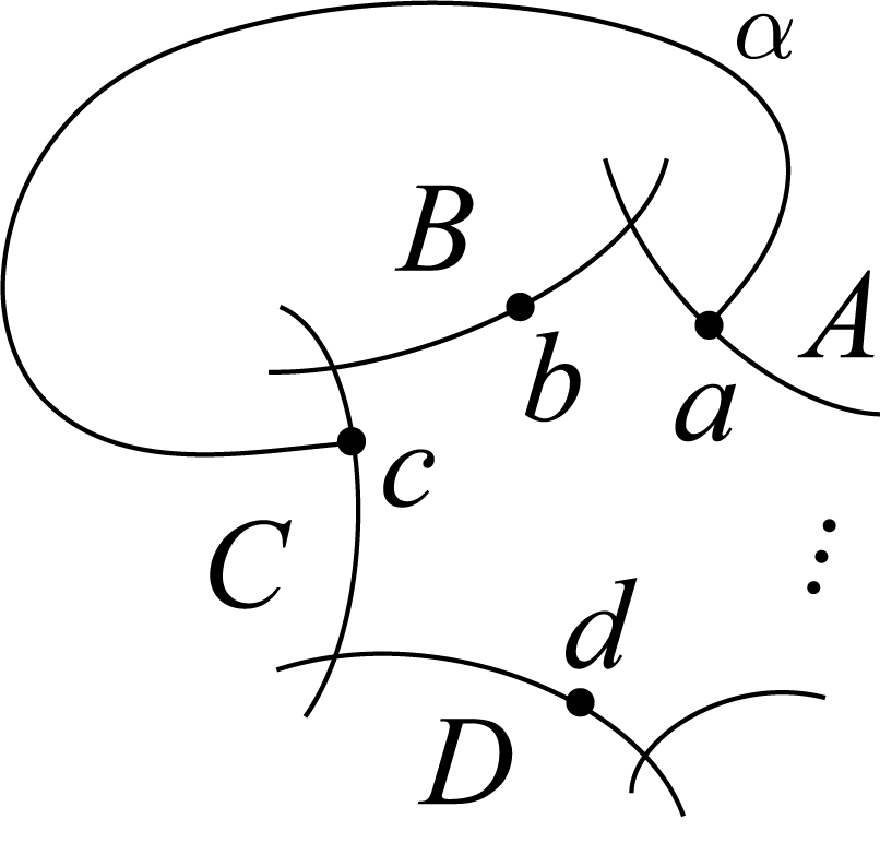
Two regions and of a link projection are said to be connected when they share a crossing on their boundaries. Otherwise, they are said to be disconnected. For example, the regions and are connected, whereas and are disconnected in Figure 1. A set of regions is said to be isolated, or an isolated-region set, if any pair of regions and are disconnected. We assume that the empty set is isolated. The isolate-region number222The isolate-region number is similar but different from the “independent region number” introduced in [8]; a crossing is fixed for ., , of a link projection is the maximum value of for all isolated-region sets of , where denotes the cardinality of . For example, the isolate-region number of the knot projection in Figure 1 is three.
We show the following theorem in Section 2.
Theorem 1.
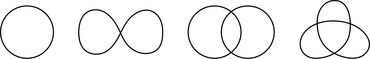
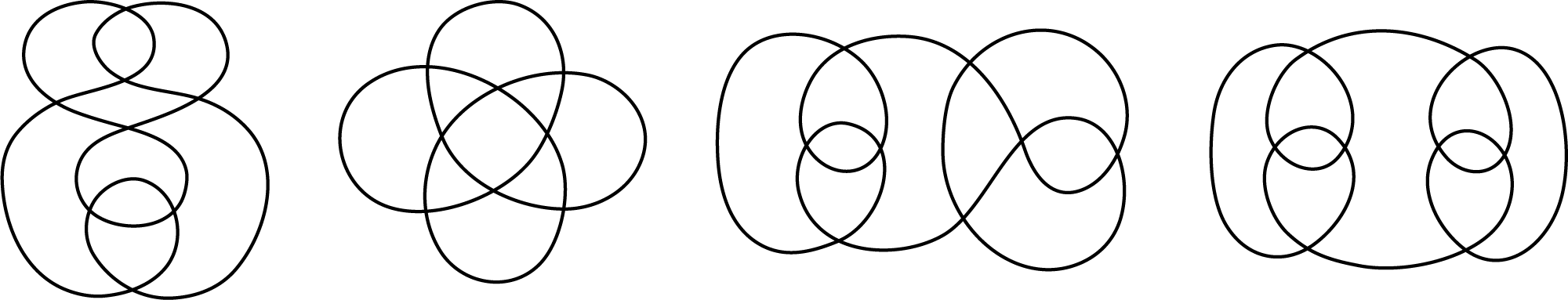
A link projection has isolate-region number one if and only if is one of the link projections shown in Figure 2.
The concept of the isolate-region number was introduced in [8] to estimate the “warping degree” of knot projections ([4, 12]). In Section 3, we investigate the warping degree and using the relation between the warping degree and the isolate-region number, we discuss the relation between the welded unknotting number of a knot diagram and the isolate-region number . We show an upper bound for (, Corollaries 4, 5) when satisfies some conditions. Generally, however, determining the isolate-region number is not easy by looking only at the link projection of large number of crossings. In Section 4, a combinatorial method to find the isolate-region number using graphs is given. Moreover, from the graphs, we can see the distribution of the isolated-region sets by considering the generating function. We give a formula and recurrence relation of generating functions for the standard projections of -torus links in Section 6.
The rest of the paper is organized as follows. In Section 2, the proof of Theorem 1 is given. In Section 3, some properties of warping degree are discussed and applied to estimate the welded unknotting number of a knot diagram. In Section 4, two graphs, the region-connect graph and region-disconnect graph are introduced to find isolated-region sets. In Section 5, the generating function of isolated-region sets are discussed. In Section 6, the generating functions for the standard projections of -torus links are discussed.
2 Proof of Theorem 1
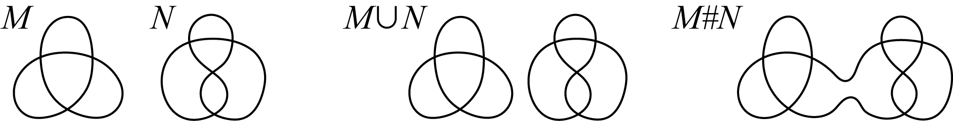
In this section, we prove Theorem 1. For link projections and , a split sum and a connected sum are link projections obtained from and as shown in Figure 3. We say a link projection is connected when is not any split sum of link projections. We say a link projection is composite when is a connected sum of two nontrivial link projections. We have the following lemma.
Lemma 1.
Every unconnected or composite link projection has .
Proof.
When is a split sum of and , take a region from and avoiding the region between them, and they are disconnected. When is a connected sum of and , take a region from -part and -part avoiding the shared two regions. Thus, we have . ∎
A crossing of a link projection is said to be reducible if it has exactly three regions around it. A link projection is reducible when has a reducible crossing. We say is irreducible when is not reducible. Since a reducible link projection can be assumed to be a connected sum when it has at least two crossings, we have the following corollary.
Corollary 1.
Every reducible link projection with two or more crossings has .
Next, we divide a link projection into two tangles by giving a circle , where intersects edges transversely. We assume each tangle is on a disk with , and call each connected portion of divided by a region of . In particular, if a region touches , we call it an open region, and otherwise we call it a closed region. We remark that any pair of closed regions in opposite sides of are disconnected. We show the following.
Lemma 2.
For any connected irreducible link projection with four or more crossings, we can draw a circle so that the tangle on each side of has a closed bigon or trigon.
Proof.
By the formula
for the number of -gons of a connected irreducible link projection shown in [1], we have .
(0) When , i.e., , draw a circle around a trigon as shown in Figure 4, (II).
Then the tangle in the figure has a closed trigon.
Since and there are at most six regions around the trigon, the tangle on the other side has a closed trigon, too.
(1) When , i.e., , draw a circle around the bigon as shown in Figure 4, (I).
Then, the tangle on the other side has closed trigons because and there are at most four regions around a bigon.
(2) When , i.e., , draw as shown in Figure 4, (I).
Since , the tangle on the other side has a closed bigon or trigon, too.
(3) When , i.e., , we consider the following cases.
(3-1) When and , choose any bigon and see (III) in Figure 4. We consider the further two cases whether or not.
(3-1-1) When , we can draw a circle as in Figure 4, (I) since we have and the bigon has only three regions around it.
(3-1-2) Suppose . Then neither nor is a bigon.
Suppose and are connected and both bigons.
Then the curve is closed with only three crossings.
Hence this does not happen.
When and are connected and either or is not a bigon, take as shown in Figure 4, (I).
Then the other side has a closed bigon, too.
(3-1-3) Suppose and they are disconnected bigons.
Then both and are -gon or more.
Take as in Figure 4, (I).
Then the other side of has closed trigons.
Suppose and are disconnected and either or is not a bigon.
Draw as in Figure 4, (I).
Then the other side has a closed bigon.
(3-2) When and , we can draw as in Figure 4, (I), because .
(4) When , i.e., , choose any bigon and see (III) in Figure 4.
(4-1) When and it is a bigon, then the curve is closed with only two crossings.
Hence this is not allowed to happen.
When and it is not a bigon, we can draw as in Figure 4, (I) since inside in the figure has at most three bigons.
(4-2) When , we can draw as shown in Figure 4, (I) since neither nor is a bigon, and inside in the figure has at most three bigons, too.
(5) When , choose any bigon and see (III) in Figure 4.
If all of are distinct bigons, then the curve is closed with only two crossings. Hence this does not happen.
We can draw as in Figure 4, (I) since inside in the figure has at most four bigons.
∎
Corollary 2.
Any link projection with or more crossings has .
Now we prove Theorem 1.
Proof of Theorem 1.
Since every unconnected projection has isolate-region number two or more by Lemma 1, it is sufficient to discuss connected projections.
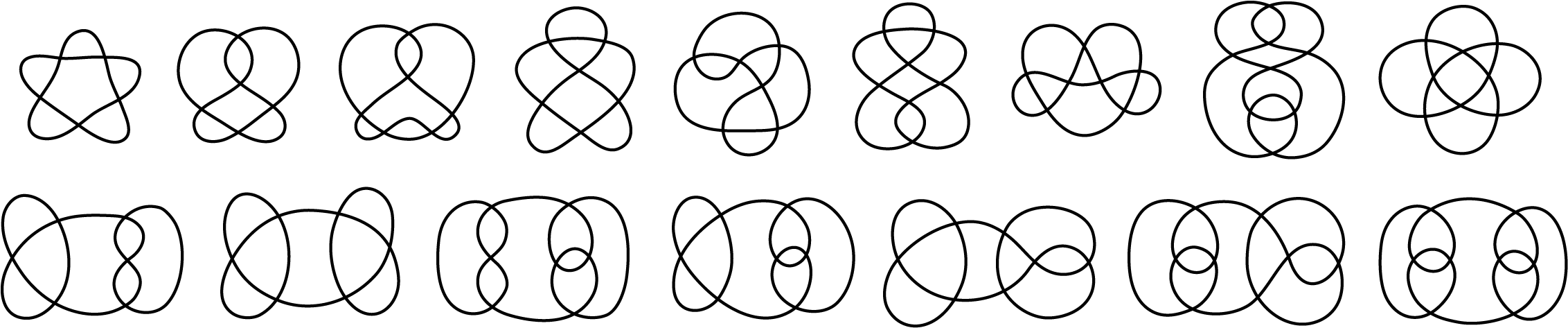
When the crossing number , there are just two link projections, the first and second knot projections in Figure 2, and they have isolate-region number one.
When , we have just two reduced link projections, the third and fourth projections in Figure 2, and they have isolate-region number one.
By Corollaries 1 and 2, there are no link projections of isolate-region number one for link projections with four or more crossings or reducible projections with two or more crossings.
∎
In addition to Corollary 2, we have the following proposition regarding the location of isolated regions.
Proposition 1.
If an irreducible knot projection has an -gon for , there is a pair of disconnected regions around the -gon.
Proof.
Take points on edges of the -gon and call the regions , as shown in Figure 5.
Since the knot projection is irreducible, we have , , .
We also have since .
(1) If and and are disconnected, they are the regions.
(2) If , we can draw a simple curve connecting and inside the region .
Since and cannot touch , they are disconnected.
(3) If and and are connected, we can draw a simple curve connecting and passing through , and one crossing shared by and .
Then, and are disconnected.
Otherwise, and must share the crossing to be connected, and we can draw a simple curve connecting and which passing through , , and .
Then, at least one of the arcs between and loses the place to go since both and have only one crossing on it.
∎
Also, we have the following corollary from Lemma 2.
Corollary 3.
Any connected irreducible link projection with or more crossings has .
Proof.
By Lemma 2, has a pair of disconnected regions of bigon or trigon, say and . Then has at most regions which are connected to either or . Since has or more regions, has at least one region, say , which is neither nor and is connected to neither nor . ∎
3 Warping degree, welded unknotting number and isolate-region number of a knot diagram
In this section, we discuss the warping degree and welded unknotting number of a knot diagram and their relations to the isolate-region number. In Subsection 3.1, we discuss the relation between the warping degrees of a knot diagram and knot projection. In Subsection 3.2, we discuss the relation between the welded unknotting number, warping degree and isolate-region number of a knot diagram.
3.1 Warping degree
Let be an oriented knot diagram with a base point on an edge. A crossing point of is said to be a warping crossing point of if we encounter the crossing as an under crossing first when we travel from with the orientation. The warping degree of , , is the number of the warping crossing points of . We can represent all the warping degrees by the “warping degree labeling” as shown in Figure 6.
The warping degree of , , is the minimal value of for all base points of ([4]). As shown in Figure 6, warping degree depends on the orientation; we have , whereas , where is with orientation reversed. In this paper, we define . For a knot diagram , we denote by the knot projection which is obtained from by forgetting the crossing information. The warping degree of , , is the minimal value of for all oriented alternating diagrams with . Although each projection has four oriented alternating diagrams (see Figure 6), the following proposition claims it is sufficient to check only one alternating diagram with two orientations.
Proposition 2.
The equality holds when is an alternating diagram with .
Proof.
As shown in [12], we have for any oriented knot diagram with a base point because the order of over crossing and under crossing is switched at every crossing. We also have for the mirror image because the crossing information is changed at each crossing. Therefore, we have , and . Hence for any alternating diagram with . ∎
A nonalternating knot diagram is said to be almost alternating if becomes alternating by a single crossing change. For almost alternating diagrams, we have the following proposition.
Proposition 3.
Let be an almost alternating diagram with . Then holds. In particular, if an almost alternating diagram has no monogons, .
To prove Proposition 3, we prepare a further formula. Since we have for any diagram , we have
for any knot diagram .
Hence, we can find the value of only from one oriented alternating diagram with by looking at the minimum and maximum values of warping degree labeling.
We prove Proposition 3.
Proof of Proposition 3.
Let be an almost alternating knot diagram which is obtained from an oriented alternating diagram by a single crossing change at a crossing .
Let (resp. ) be a portion of from a point just after the over crossing (resp. the under crossing) of to a point just before the under crossings (resp. the over crossing) of .
Let (resp. ) be the corresponding portions of to (resp. ).
Each warping degree labeling on is smaller than the corresponding labeling on by one because becomes a non-warping crossing point for base points on by the crossing change at ([5, 13]).
In the same way, each labeling on is greater than by one.
Let .
Then we have , and .
(1) When both and have crossings, their warping degree labeling are consisting of and .
After the crossing change, the labels on are and the labels on are .
Hence and , and therefore .
(2) When has no crossings and has crossings,
the label of is only and the labels of are , and the labels of is and that of are .
Hence , and .
(3) When has crossings and has no crossings,
the labels of are and that of is only , and the labeling of are and that of is .
Hence , and .
(4) When neither nor has crossings, then , and is not an almost alternating diagram.
Therefore, we have , where .
In particular, if has no monogons, then both and must have crossings for any crossing , and this case applies (1).
∎
Next, we show the following proposition.
Proposition 4.
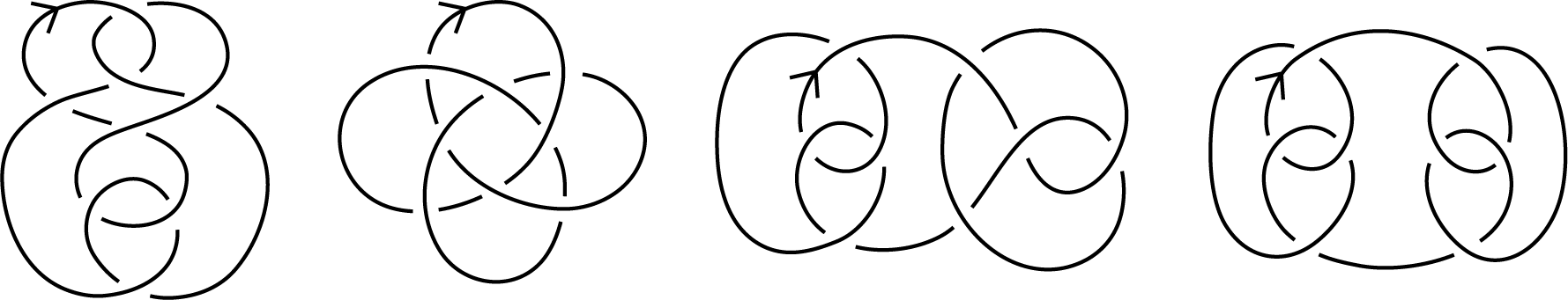
Let be an irreducible knot projection with . The inequality holds for any knot diagram with if and only if is neither of the four projections illustrated in Figure 7.
To prove Proposition 4, we prepare Lemmas 3, 4, 5. All the irreducible knot projections with warping degree 1 and 2 are determined in [11].
Lemma 3.
The following lemma gives an upper bounds for and .
Lemma 4.
The inequality holds for any knot diagram with . The inequality holds for any knot projection with .
Proof.
By the inequality shown in [12], we have , and therefore . Since this also holds for alternating diagrams , we have . ∎
The span, , of an oriented knot diagram is defined to be the difference . By definition, we have . Also, we have the following.
Lemma 5.
[13] The span is one if and only if is an alternating diagram.
Using the above lemmas, we show Proposition 4.
Proof of Proposition 4. We show that there exist no non-alternating diagrams with such that under the condition.
When or , we have by Lemma 4, and there are no diagrams with satisfying by Lemma 4.
When or , we have by Lemmas 3, 4, and there are no diagrams satisfying by Lemma 4.
When , or by Lemmas 3, 4.
There are no diagrams with satisfying by Lemma 4.
When , each oriented alternating diagram with has warping degree labeling or .
There are no nonalternating diagrams with such that the minimal label is greater than and the maximal labeling is smaller than , because .
When , or by Lemmas 3, 4.
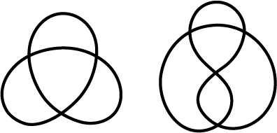
When , is one of the four knot projections depicted in Figure 7 by Lemma 3.
For each knot projection , we have a diagram with such that as shown in Figure 10.
When , the warping degree labeling on is or , and there are no nonalternating diagram such that the minimal label is greater than and the maximal label is less than since .
When , or by Lemmas 3, 4.
There are no diagrams such that by Lemma 4.
When , each oriented alternating diagram has warping degree labeling or .
There are no nonalternating diagrams such that the minimal label is greater than and the maximal label is less than since . ∎
3.2 Welded unknotting number
In this subsection, we apply results in Subsection 3.1 to a study of welded knot diagrams. A welded knot diagram is a diagram obtained from a classical knot diagram by replacing some classical crossings with “welded crossings”. A welded knot ([3, 9]) is the equivalence class of welded knot diagrams related by classical and virtual Reidemeister moves and the over forbidden move. The welded unknotting number, , of a welded knot diagram is the minimum number of classical crossings which are needed to be replaced with a welded crossing to obtain a diagram of the trivial knot ([7]). Let be a classical knot diagram. It is known that ([6, 7, 10]), as a relation between the welded unknotting number and the warping degree. On the other hand, the inequality , the relation between the warping degree and the isolate-region number, was shown in [12]. For a knot diagram , let , where . With Propositions 3, 4, we have the following corollaries which are estimations of the welded unknotting number in terms of isolated regions.
Corollary 4.
Let be an almost alternating diagram. We have .
Corollary 5.
Let be an irreducible knot diagram of such that is neither of the projections in Figure 7. We have .
4 Region-connect graph and its complement
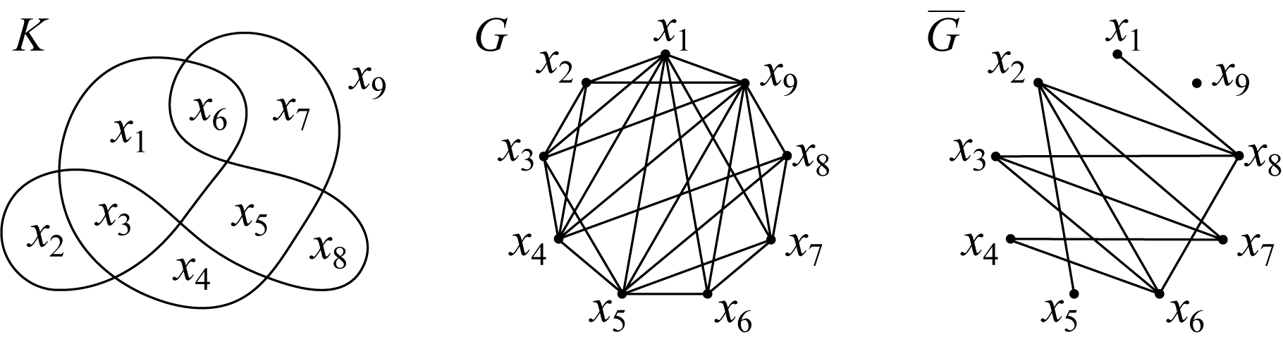
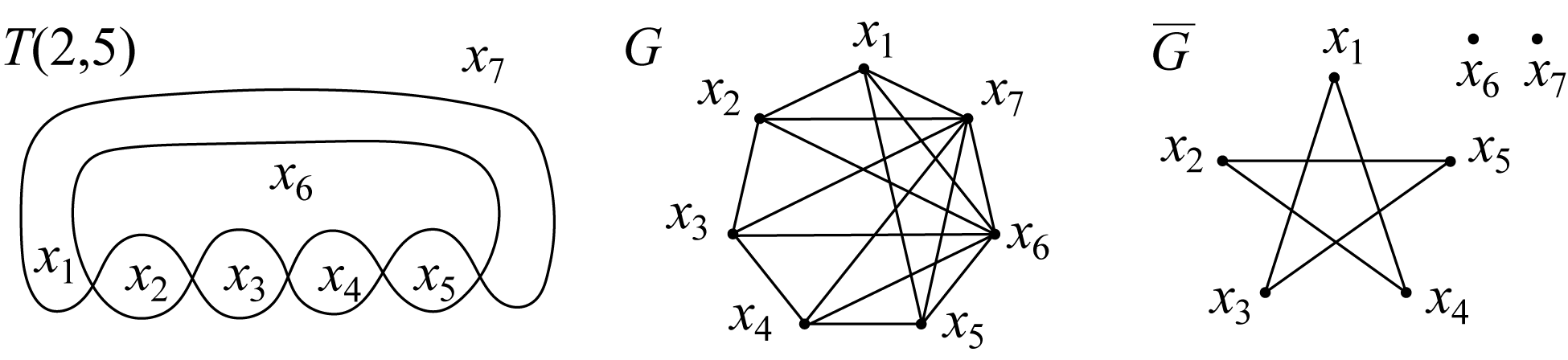
In this section, region-connect graph and region-disconnect graph are defined and investigated. Then an algorithm to find the isolate-region number is given. For a graph , we say a graph is a subgraph of and denote by if or is obtained from by deleting some vertices and edges. For a link projection with regions, give labels to the regions. The region-connect graph of is the graph with the vertices labeled and the edges for all the pairs of connected regions and (see Figure 11). The region-disconnect graph, , of is the complement graph of . By definition, represents which pairs of regions are disconnected. Then we can find the isolated-region sets of by looking at as follows. Find a subgraph of which is a complete graph . Since the corresponding regions to the vertices of are disconnected each other in , the set of them is isolated. Moreover, the maximum size of a complete graph is identical to the isolate-region number . For example, we obtain for the knot projection in Figure 11 because the graph includes and does not include for .
5 I-generating function
In this section, we explore the generating functions for isolate-region sets of a link projection. Let be a link projection. Let be the set of all regions of . Let be the power set of . Now we want to know how isolated-region sets are distributed in . First, each element is determined by the choices whether each region is taken or not. Hence, all the elements in can be seen as the terms of the following polynomial.
where or in denotes if the region is chosen or not respectively. For , delete the terms which include the pair of connected regions, i.e., the pair of the letters which are connected in . Then we obtain a polynomial which represents all the isolated-region sets. Since we want to know just the number of isolated-region sets, replace each with . Then, we obtain the generating function for for isolated-region sets . In this paper, we call the i-generating function of . By definition, the maximum degree, , indicates the isolate-region number of . We have the following proposition.
Proposition 5.
For each i-generating function of a connected link projection with crossings, and . All the terms from degree 0 to are nonzero.
Proof.
We notice that each coefficient is the number of isolated-region sets consisting of regions. In terms of the region-disconnect graphs , is the number of with . The first claim is obvious from the fact that we have one and the number of regions of is . For the second claim, when includes a complete graph , then also includes because . ∎
For connected irreducible link projections, we have an upper and lower bounds for as follows333We note that Proposition 6 does not include Corollary 2 because the proposition claims just when ..
Proposition 6.
Let be a connected irreducible link projection with crossings and let be the i-generating function of . We have
Proof.
The upper bound is , the number of edges of since . For the lower bound, let be the regions of . Suppose is a -gon. Then has at most regions around . For each region , the number of regions which is disconnected to is at least , where implies the number of all regions of . In total, we have
where we divided the summation by 2 to fix the double counting. Since we have
for connected irreducible link projections, we have
∎
6 I-generating functions of -torus link projections
In this section, we investigate the i-generating functions for the standard projections of -torus links, and prove the following theorem.
Theorem 2.
The i-generating function of a standard projection of the -torus link is
For a standard projection of a -torus link, give labels of regions as shown in Figure 12.
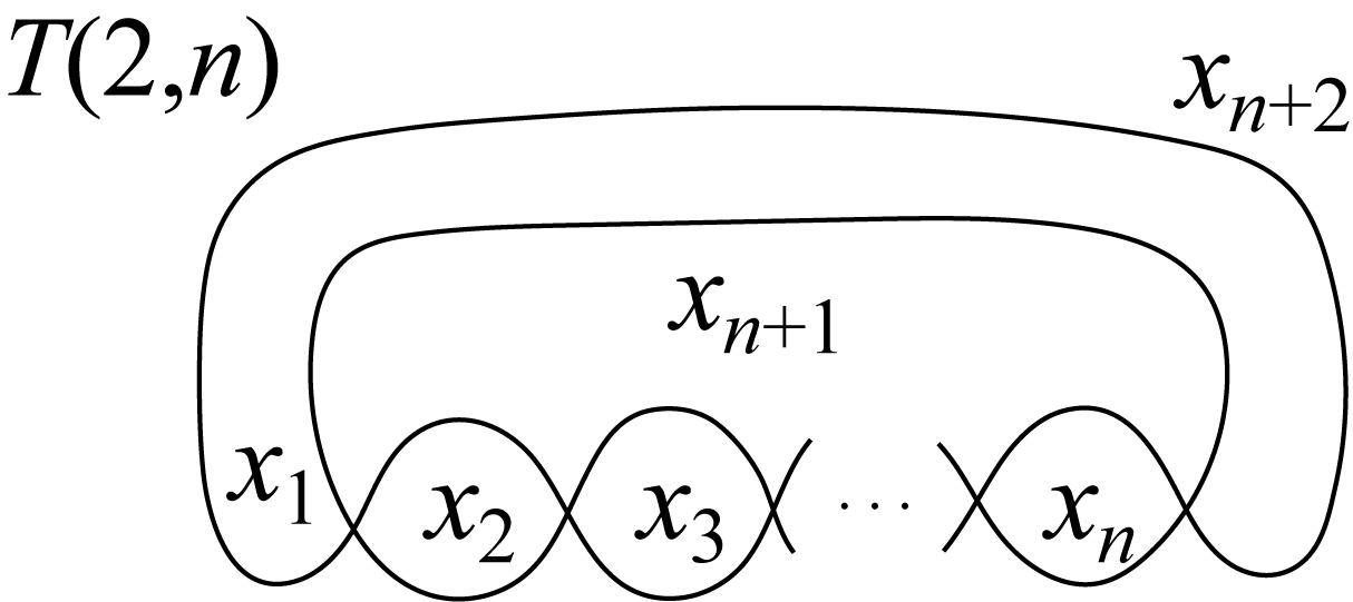
We notice that the th and th regions are connected with all the other regions. Also, when , each region from the 1st to th is connected to the four regions, the th and th regions and the neighboring two bigons. In the region-connect graph , therefore, the th and th vertices have degree , and the others have degree four. As for , the th and th vertices have degree zero, and the others have degree . Moreover, in , the vertices forms a complete graph missing the following edges, . For example, when , we have and as shown in Figure 13, and the polynomials , , and .
To prove Theorem 2, we prepare a (perhaps well-known) formula.
Lemma 6.
Suppose there are white balls in a line. Denote by the number of cases to paint of balls red so that the painted balls are not next to each other. Then,
Proof.
At first, suppose white balls in a line. Then there are rooms between balls or on a side. The number of ways to put the painted red balls there is . ∎
Now we show Theorem 2.
Proof of Theorem 2. Let be the region-disconnected graph of with the regions labeled as in Figure 12. Note that the th and th vertices have degree zero. For the subgraph of consisting of the vertices and the edges, we discuss how many complete graphs are included.
Let be the i-generating function. For the maximum degree, we have because we can take non-neighboring vertices and cannot for from , where we say and are neighboring when or .
For coefficients, we have as the empty set of vertices. We have , the number of vertices (or ) of , as mentioned in Proposition 5. We have , the number of edges (or ) of . More precisely, fix a vertex . Then has choices of vertices to form an edge in . Remark that cannot be connected with the neighboring vertices. Multiple by because we can consider the same thing for the vertices. Divide it by two since each edge is double counted. Hence, we have .
Next, for , we obtain in the following way. Fix a vertex . Then has non-neighboring edges and has choices to take other vertices to form so that any pair of vertices is not neighboring. Multiple by , and divide it by since each is counted times. Then,
This holds when , too. ∎
The i-generating functions of are listed below for to .
We have the following formula.
Proposition 7.
For the i-generating functions of , we have
for .
Proof.
Let be the coefficient of of . When , the th coefficient of is , that of is , and the th coefficient of is . Hence,
Using the formula , we have and
For , , and . Hence, we have and for , and holds for . ∎
From Proposition 7, we have a recurrence relation about the number of isolated-region sets.
Corollary 6.
For the i-generating function of of , we have
Acknowledgment
The authors thank Professor Rama Mishra for her support and encouragement. The second author’s work was partially supported by JSPS KAKENHI Grant Number JP21K03263.
References
- [1] C. C. Adams, R. Shinjo and K. Tanaka, Complementary regions of knot and link diagrams, Ann. Comb. 15 (2011), 549–563.
- [2] K. Ahara and M. Suzuki, An integral region choice problem on knot projection, J. Knot Theory Ramifications 21 (2012), 1250119.
- [3] M. H. Fenn, R. Rimányi and C. Rourke, The braid-permutation group, Topology 39 (1997), 123–135.
- [4] A. Kawauchi, Lectures on knot theory (in Japanese), Kyoritsu Shuppan (2007).
- [5] A. Kawauchi and A. Shimizu, Quantization of the crossing number of a knot diagram, Kyungpook Math. J. 55 (2015), 741–752.
- [6] Z. Li, F. Lei and J. Wu, On the unknotting number of a welded knot, J. Knot Theory Ramifications 26 (2017), 1750004.
- [7] T. Mahato, R. Mishra and S. Joshi, Non-triviality of welded knots and ribbon torus-knots, preprint (arXiv:2404.00436).
- [8] A. Ohya and A. Shimizu, Lower bounds for the warping degree of a knot projection, J. Knot Theory Ramifications 31 (2022), 2250091.
- [9] C. Rourke, What is a welded link?, Intelligence of low dimensional topology 2006, 263–270, Ser. Knots Everything 40 (2007), World Sci. Publ., Hackensack, NJ.
- [10] S. Satoh, Virtual knot representation of ribbon torus-knots, J. Knot Theory Ramifications 9 (2000), 531–542.
- [11] A. Shimizu, Prime alternating knots of minimal warping degree two, J. Knot Theory Ramifications 29 (2020), 2050060.
- [12] A. Shimizu, The warping degree of a knot diagram, J. Knot Theory Ramifications 19 (2010), 849–857.
- [13] A. Shimizu, The warping polynomial of a knot diagram, J. Knot Theory Ramifications 21 (2012), 1250124.