MD-NOMAD: Mixture density nonlinear manifold decoder for emulating stochastic differential equations and uncertainty propagation
Abstract
We propose a neural operator framework, termed mixture density nonlinear manifold decoder (MD-NOMAD), for stochastic simulators. Our approach leverages an amalgamation of the pointwise operator learning neural architecture nonlinear manifold decoder (NOMAD) with mixture density-based methods to estimate conditional probability distributions for stochastic output functions. MD-NOMAD harnesses the ability of probabilistic mixture models to estimate complex probability and the high-dimensional scalability of pointwise neural operator NOMAD. We conduct empirical assessments on a wide array of stochastic ordinary and partial differential equations and present the corresponding results, which highlight the performance of the proposed framework.
Keywords Deep learning Stochastic simulator Uncertainty Operator learning
1 Introduction
Differential equations (DE) hold a pivotal position in engineering and scientific endeavors, constituting fundamental tools for inquiry and practical application. These equations serve as primary vehicles for elucidating the behavior of intricate physical systems through mathematical formulations. These formulations typically encapsulate the inherent dynamics and relationships within the systems under examination, often presenting a concise and condensed representation. Moreover, they furnish a framework essential for forecasting the intricate interactions within these systems. Even though DEs are extensively used across various scientific disciplines, obtaining analytical solutions, particularly for partial differential equations (PDEs), is often challenging and usually unattainable in practical engineering contexts marked by complex geometries, nonlinearities, and boundary conditions. Consequently, for solving PDEs in such scenarios, one resorts to numerical analysis [12, 23] with simulators based on numerical methods such as finite difference [18], finite element [25], and finite volume [17] techniques, which are employed to approximate the solutions for these equations. However, even when employing these methods, solving a PDE can evolve into a complex and time-intensive undertaking, especially in cases where complete knowledge of all parameters and boundary or initial conditions (BCs/ICs) is lacking. Furthermore, the incorporation of simplifications and assumptions to address gaps in the understanding of partially known parameters and BCs/ICs (epistemic uncertainty) inevitably might result in numerical approximations that deviate from the physical reality. Moreover, many physical systems [28, 14] inherently entail uncertainty that cannot be fully captured by deterministic models, and via extension, by deterministic simulators. However, this challenge is usually addressed by employing stochastic differential equations (SDEs), which are commonly utilized to articulate the governing physics and integrate associated uncertainty by incorporating both deterministic and stochastic influences.
While stochastic differential equations (SDEs) furnish us with the ability to model systems characterized by uncertainty, such modeling necessitates the utilization of stochastic simulators — computational models employing numerical techniques tailored for SDEs [14]. Furthermore, due to the intrinsic randomness embedded within SDEs, the output of these simulators, with a fixed set of input parameters, emerges as a random variable adhering to an unknown conditional distribution. Moreover, to describe this output distribution, stochastic simulators must be repeatedly evaluated for the same input parameters to obtain the associated statistics and probability density functions (PDFs). Consequently, while SDEs provide a framework for tackling uncertainty in physical systems, the computational expense involved in numerically modeling these equations is increased in comparison to deterministic DEs.
To tackle the challenge of computational cost associated with stochastic simulators, the construction of surrogate models, which are adept at approximating the input-output relationships while maintaining computational efficiency, for these simulators has emerged as a prudent and pragmatic option. The field of surrogate modeling has garnered appreciable attention in the recent past. Within the framework of strategies inclined towards traditional methods for surrogate modeling of stochastic simulators, diverse methodologies have been investigated and refined. These include generalized additive models [11], generalized linear models [22], [7], kernel density estimators [10, 8], Gaussian processes [4], polynomial chaos expansions [2], and more sophisticated models that build upon and refine standard surrogate modeling approaches such as generalized lambda distribution-based models [35, 34] or stochastic polynomial chaos expansions [36]. However, certain limitations are associated with these methods: some are susceptible to the curse of dimensionality [32], others necessitate data to conform to specific requirements [2], some have intricate implementations [34], while others demand numerous replications for identical input parameters [35]. Additionally, certain methods impose restrictions on the shapes of response distributions that can be emulated [11, 22]. Furthermore, with the advancement of machine learning, contemporary deep learning-based methods for surrogate modeling of stochastic simulators have drawn noticeable focus. These approaches encompass various techniques, such as normalizing flow-based models [21], generative adversarial networks (GANs) [33], neural stochastic differential equations [13], surrogate modeling through optimal transport and projection pursuit [3], and gray-box methodologies like combining conditional generative moment matching networks (CGMMN) [26] with partially known SDEs [5], or integrating neural networks (NNs) with numerical integrator-motivated loss functions to identify drift and diffusivity functions in SDEs [6]. Nonetheless, it’s worth noting that CGMMN and GAN-based models can pose challenges during training, and normalizing flow-based models require significant computational resources [3].
A more recent development in deep learning and surrogate modeling for DEs has been the introduction of NN architectures termed neural operators [15, 19, 29, 20, 31], which, by utilization of available data, can approximate the mapping between two continuous functions that belong to infinite-dimensional function spaces. Furthermore, the usage of some of the neural operator architectures is limited to specific types of meshes [19, 31], while others are mesh-independent and leverage a pointwise approximation strategy [29, 20]. Additionally, Fourier and Wavelet neural operators [19, 31] utilize discrete convolutions, which incur escalating computational costs as spatial dimensions increase. However, mesh-independent pointwise architectures such as NOMAD [29] and DeepONet [20] establish a separation between sensor measurements/parametric inputs and spatial/temporal/spatiotemporal location by supplying the former and latter to different sub-networks, while simultaneously linking the two subnetworks through some type of reconstruction procedure to finally obtain the output at the supplied spatial/temporal/spatiotemporal location. Moreover, the pointwise nature of NOMAD and DeepONet also aids in scalability to higher dimensional problems. However, while the aforementioned neural operator architectures, originally implemented as deterministic models, are more suitable as surrogate models for non-stochastic DEs, probabilistic variants of neural operators such as variational autoencoding NOMAD [29] and variational Bayes DeepONet [9] have also been introduced. Nevertheless, variational methodology-based deep learning models encounter numerous challenges including imprecise likelihood (unless invertible NNs are used), complexity in modeling intricate probability distributions, and training instabilities. To this end, we propose Mixture Density NOMAD (MD-NOMAD), a novel framework that blends the formalism of mixture density modeling [1] with the neural operator framework NOMAD., and functions as a surrogate model/operator learning framework for both stochastic ordinary and partial differential equations. Furthermore, the key characteristics of MD-NOMAD include:
-
•
Due to its mesh-independent and pointwise nature, MD-NOMAD is adaptable for scaling, as a surrogate model, to high-dimensional problems solved on arbitrary meshes.
-
•
MD-NOMAD is easy to implement, employs standard optimization techniques, i.e, does not require specialized interventions such as reparameterization trick or stochastic gradient variational Bayes estimator, and is computationally less expensive and easy to train as compared to generative models such as normalizing flows, GANs, and variational networks.
-
•
With an appropriate number of mixture components, MD-NOMAD is capable of modeling complex probability distributions such as multimodal, skewed, or other non-Gaussian distributions.
-
•
Since the PDFs of the employed mixture distribution are typically accessible, the requirement for employing Monte Carlo (MC) methods to estimate the statistics and PDF of the conditional output distribution during the inference stage is eliminated, and these can be computed analytically once the parameters of the mixture components are obtained from MD-NOMAD for a given input.
-
•
MD-NOMAD can be used to construct a surrogate model for one-shot uncertainty propagation for DEs.
The paper is structured as follows: Section 2 outlines the problem statement, while Section 3 offers an overview of the necessary background for comprehending the mathematical foundations of the proposed framework, including a brief review of mixture density networks and NOMAD. Section 4 delves into the details of the proposed framework. In Section 5, we present four examples to illustrate the performance of the proposed framework. Finally, Section 6 presents the concluding remarks.
2 Problem statement
Before exploring the problem statement, we initiate by introducing certain notations. Consider a fixed -dimensional domain bounded by with input function in the Banach space and output function in the Banach space , where . For traditional deterministic simulator, a nonlinear differential operator can be defined as follows:
| (1) |
In the context of pointwise mapping, considering a point within the domain , the output function produces a real value, i.e., . Additionally, in deterministic simulations, identical and inputs consistently result in the same output function values. However, with probabilistic or stochastic simulators, the uncertainty arising from the inherent characteristics of the system or insufficient knowledge thereof leads to varying output function values for a given and . Therefore, to characterize the behavior of the output function for a stochastic simulator, random variable has to be introduced. Based on this, the nonlinear differential operator for stochastic simulators can be expressed as follows:
| (2) |
where signifies the event space of the probability space , encapsulating the randomness, and is stochastic output function. Compared to deterministic simulations, stochastic simulators incur higher computational costs as numerous simulator runs have to be performed for a given set of inputs for a good characterization of PDFs for the simulator’s output. Therefore, this paper aims to devise a mixture density-based operator learning framework for the construction of surrogate models tailored for stochastic simulators.
3 Preliminaries
3.1 Mixture density networks
Mixture Density Networks (MDNs) were introduced by Bishop [1] as an NN-based framework for modeling complex conditional probability distributions. Considering, as an input to the network, MDNs model the conditional distribution , i.e, the probability distribution of model output given input , using a mixture of probability distributions. Mathematically, the mixture-based approximation of conditional distribution using NNs can be expressed as
| (3) |
Here, is the mixing coefficient of the -th component and represents the PDF of the -th component, where the parameters of PDF and mixing coefficients are in turn parameterized by NN parameters and also depend on the input . Furthermore, any parametric family of probability distributions, for example, Gaussian, Laplacian, beta, exponential, or others, can be used as the mixture components, and the choice is contingent upon the characteristics of the problem being modeled.
During training, the parameters of MDN are optimized by utilizing the input-output training data pairs to predict the mixture components parameters ( and ). This is typically achieved by minimizing the negative log-likelihood loss function. Furthermore, during inference, the MDN can generate samples from the conditional distribution for a given input by sampling from the mixture-based distribution or can provide PDFs or requisite statistics using analytical computations based on the mixture component parameters.
3.2 NOMAD
A widely adopted approach for constructing operator learning frameworks, as proposed by Lanthaler et al. [16], involves composing three approximation maps. By employing this composition, the operator defined in Equation 1 can be approximated as follows:
| (4) |
Here, represents an encoding map that transforms a continuous function to its evaluation at locations. The encoder is succeeded by the application of the approximation map, represented by , which maps pointwise function evaluations to a latent space with dimension . Generally, is an NN. The composition of the encoding and approximation maps denoted as , is referred to as the branch network. This is followed by the reconstruction or decoding map, denoted as , which maps the finite-dimensional latent feature representation to the output function. In a DeepONet, the reconstruction map is a dot product between a set of functions, , parameterized by an NN (also known as the trunk network) and , where and . This can be expressed as
| (5) |
However, the utility of linear reconstruction maps is constrained by the Kolmogorov n-width [29, 24]. To address this limitation, Seidman et al. [29] introduced a nonlinear reconstruction/decoding map that is parameterized by an NN. This map can be expressed as follows:
| (6) |
where, is a deep neural network. Ultimately, the fusion of the nonlinear decoder with the branch network constitutes the NOMAD architecture.
4 Proposed framework
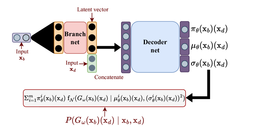
As discussed in Section 3, while a deterministic NOMAD can effectively learn a mapping from input function evaluations to output function values, it cannot directly model the mapping for a stochastic operator, which typically necessitates the estimation of the PDF of the output function. Hence, to address this, we combine the pointwise operator learning NOMAD framework with the mixture density-based formalism to arrive at the mixture density NOMAD (MD-NOMAD) architecture. This MD-NOMAD framework, by design, enables the estimation of the conditional probability distribution for a stochastic output function associated with the input function given a sensor value . While various parametric distributions could be considered for the mixture components, for this study, we focus solely on the Gaussian distribution due to its simplicity and interoperability. Thus, within this framework, an analog to in Equation 3 is represented as , denoting a Gaussian distribution with mean and standard deviation (or variance ) for the -th mixture component, where the mean, standard deviation/variance, along with the mixing coefficient, are parameterized by a NOMAD with parameters . In addition, to ensure that the standard deviation/variance is non-negative, softplus activation function is applied to the NOMAD predicted component parameters for standard deviation/variance. Furthermore, and represent the inputs to the branch and decoder network, respectively. A schematic of the MD-NOMAD’s architecture is illustrated in Figure 1.
The optimization of the trainable parameters of MD-NOMAD, given input-output data pairs, which enables it to predict the mixture parameters, is accomplished through the minimization of an appropriate loss function . In addition, in surrogate models for stochastic simulators, which inherently involve probabilistic elements, one typically employs probabilistic loss functions like Kullback-Leibler divergence, maximum mean discrepancy, or negative log-likelihood. However, in the context of MD-NOMAD, our focus lies in determining the parameters of the component distribution that maximize the likelihood of observed or provided data given these parameters. Consequently, in the current scenario, the minimized loss function is the negative log-likelihood, expressed as:
| (7) |
where is a Gaussian probability density function. It is key to note that MD-NOMAD inherits scalability characteristics from NOMAD (or DeepONet) architectures owing to their point-wise approach, which is particularly beneficial for high-dimensional problems. Additionally, the complexity of our architecture, specifically, the final layer involving parameters of the mixture densities, is contingent upon the number of components employed. This, in turn, is influenced by the complexity of the probability distribution at sensor locations. Moreover, once the model can predict the parameters of component distributions for given inputs upon successful optimization, the computations for statistics and PDFs for the model-predicted conditional output distribution can be done analytically. In addition, throughout this study, we adopt a replication-based experimental design to generate training and validation data. Initially, we create a distinct set of input parameters by sampling from predetermined parameter ranges. The size of this set is represented by , while denotes the number of replications for each input parameter. Together, this collection of unique input parameters and their replications constitutes the experimental design. Subsequently, for each point within the experimental design, a corresponding target output is generated utilizing an appropriate stochastic simulator tailored to the specific problem under investigation.
5 Results and discussion
In this section, we present an empirical evaluation of the performance of the proposed model across various stochastic differential equations, encompassing both linear and nonlinear formulations, alongside an analytical benchmark problem. Furthermore, given that the proposed framework involves parameter prediction for a mixture of Gaussian distributions, the predicted PDFs and statistics by the proposed model for the target variables in all examples presented in this article, given a specific input set, rely on analytical computation rather than MC-based sampling methodologies. For example, the predicted PDF is obtained by computing the sum of Gaussian PDFs (equal to the number of components used) weighed by the corresponding mixture weights and parameterized by the corresponding mean and standard deviation/variance values predicted from MDN-NOMAD. Mathematically, the computation of a PDF for a particular set of , , and values predicted by an -component MD-NOMAD can be expressed as follows
| (8) |
In addition, we showcase the utility of our model for one-shot uncertainty propagation within a setting based on 2-dimensional stochastic partial differential equations (SPDEs).
5.1 Stochastic Van der Pol equation
The Van der Pol equation, characterized by non-conservative dynamics and nonlinear damping, is utilized across diverse domains such as biology, electronics, physics, and economics. However, in this example, we utilize the stochastic variant of this equation, which can be mathematically expressed as follows
| (9) | ||||
Here, is used to represent the Wiener noise. We are only interested in the construction of a surrogate for the temporal evolution of , and thus, we ignore . One of the interesting aspects of choosing the mentioned parametric sampling range for is that this choice allows for bifurcation in our quantity of interest (QOI), i.e., , as it evolves with time, and therefore, the corresponding PDF undergoes a transition from being unimodal to being bimodal. The stochastic Van der Pol equation is solved using order 1.0 strong Stochastic Runge-Kutta algorithm [27], and the python-based package sdeint is leveraged. For this example, the experimental design is contingent on stochastic noise strength , i.e, we sample values for from the decided sampling distribution, replicate them times, and solve the SDE for each value to generate the required dataset.
We use the MD-NOMAD to learn the mapping from to . The mapping is eventually employed to obtain the probability density function . We use a small two-layered FCN for the branch network and a comparatively larger 4-layered FCN for the decoder network. In addition, the stochastic noise strength is employed as an input to the branch net whereas is used as the augmenting input to the decoder network. Due to our choice for the experimental design, the complete dataset consists of solution trajectories. Furthermore, the full dataset is randomly split into training and validation datasets with a size ratio. The Adam optimizer is employed for the mini-batch-based training with a suitable learning rate and schedule, while the number of training epochs and mixture components is set to and respectively. Also, the number of layers in the branch and decoder network along with the optimizer and the train-validation split is kept the same, unless stated otherwise, for different problems assessed in this study. In addition, the number of realizations and replications used for the current example are and , respectively.
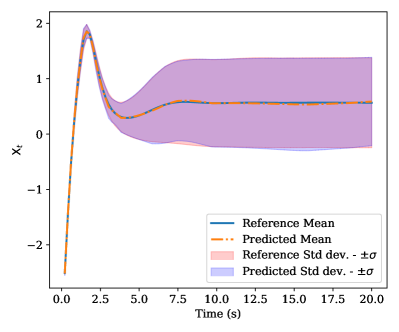
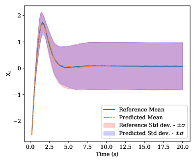
Finally, to assess the performance of the trained MD-NOMAD, we perform a comparison between the reference distribution and statistics with the model-predicted PDF and the statistics. We carry out this comparison on two randomly chosen values for stochastic noise strength and , which are not present in the training or the validation dataset. Specifically, two types of pictorial comparisons are performed — the first one being the comparison between the predicted PDF and the reference distribution for at a few different temporal locations through the solution time span to ascertain how well the proposed model performs in capturing multiple moments of the desired distribution, and the second one is the comparison between the reference statistics, i.e., mean and standard deviation, and the predicted statistics for the entire solution time-span. Both the reference distribution and corresponding statistics are obtained from the empirical distribution of replications. We again emphasize that as the output of MD-NOMAD is the parameters for a mixture of Gaussian distribution, the predicted PDF and statistics are obtained in an analytic way obviating the need for a large number of MC simulation (MCS) runs. The results for comparison between the predicted PDF and the reference distribution at different temporal locations are presented in Figure 2, while the comparison between the temporal evolution of predicted and reference statistics is presented in Figure 3. It can be observed from Figure 2 that MD-NOMAD can predict PDFs for with reasonable accuracy even after the bifurcation, i.e., where the PDF transitions from unimodal to bimodal.


5.2 N-dimensional stochastic Lorenz-96
The stochastic Lorenz-96 system represents a nonlinear set of stochastic ordinary differential equations, offering a simplified model to capture atmospheric dynamics, particularly the intricate multi-scale interactions. We consider the -dimensional stochastic Lorenz-96 system, expressed as:
| (10) |
where denotes cyclic indices. For this illustration, we aim to construct a surrogate for all -components of the state variable . The trajectories for the Lorenz-96 system are generated utilizing the Euler-Maruyama method with a time step over the period . In addition, the experimental design is based on the diffusion coefficient , which is sampled from a uniform distribution with realizations and replications. Despite the introduction of a general -dimensional system, our investigation confines itself to two scenarios: and . It’s important to recognize that this system also experiences bifurcation, and the PDFs for different components of transition from densities with sharper peaks to diffused ones as time progresses.
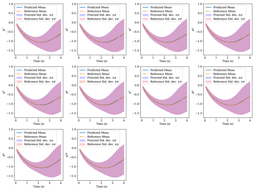
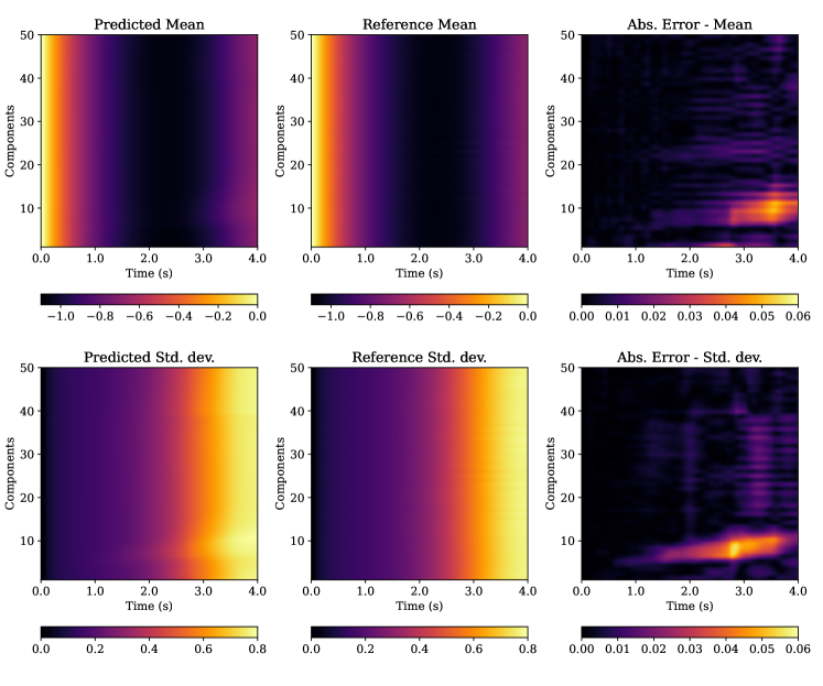
The MD-NOMAD, for this system of equations, is used to construct a surrogate for the following mapping: . We use as the branch network’s input, while are concatenated to latent branch network outputs to form the inputs for the decoder network. As we employ a pointwise NN architecture in this study, we require conditioning variables for different components of the -dimensional Lorenz equation. In this example, acts as a conditioning variable for enabling MD-NOMAD to construct the required surrogate map for a particular component. It is important to understand that has to be scaled suitably before supplying it to the decoder network. We scale by dividing the size of Lorenz’s system, i.e., . Furthermore, during the preprocessing of the training and validation dataset, the system dynamics trajectories are temporally subsampled by a factor of to mimic a setting with sparser data availability. The number of components used for the Gaussian mixture and the total number of training is chosen to be and for the dimensional system, whereas, for the dimensional system these are set to and . For conciseness, the results containing the predictions for the PDFs at different times, which can be found in Figure 4 and Figure 5, are presented for some selected components. Furthermore, the results containing the statistics are presented in Figure 6 and Figure 7. The results correspond to a case with stochastic noise strength , which is not a part of the training and validation dataset. Furthermore, the reference distribution and corresponding statistics are obtained from the empirical distribution of replications.


5.3 Bimodal analytical benchmark
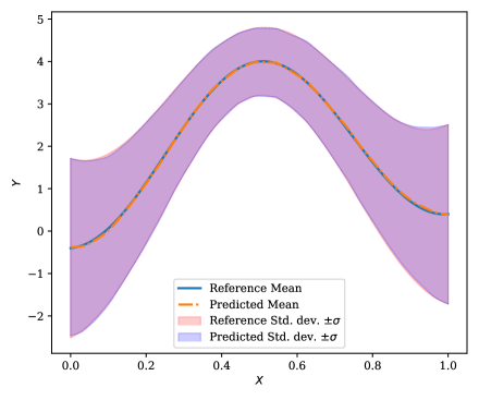
In this example, we extend a complex analytical case introduced by Zhu and Sudret [36] by incorporating additional parametric dependence on mixture weights. The target distribution is defined as:
| (11) |
Here, denotes a normal PDF with a nonlinear mean function with respect to and a standard deviation of . The parameter parameterizes the mixture coefficients, and is an input vector of -values consisting of uniformly spaced points between and . The target PDF is a mixture of two Gaussian PDFs. The experimental design is based on the mixture coefficient parameter , which is sampled from a uniform distribution with realizations and replications. The number of training epochs and the number of mixture component is equal to and respectively. The objective is to construct the following mapping with MD-NOMAD: . The complementary pair is used as an input to the branch network, while is appended to the latent output of the branch network to create an input for the decoder network.
For the evaluation of our framework in a testing scenario, we set to be equal to . Interestingly, the resulting conditional distribution transitions from being bimodal for to unimodal for and again back to bimodal for [36]. Additionally, the reference PDFs used for comparison with the predicted PDFs are obtained analytically using Equation 11. The pictorial illustration of the performance of MD-NOMAD is provided in Figure 8 and Figure 9.

5.4 2-dimensional SPDE: One-shot uncertainty propagation
Consider the following 2-dimensional elliptic PDE:
| (12) |
with representing the diffusion coefficient. This equation operates within a unit square domain, where , and it is adapted from Tripathy and Bilionis [30]. Furthermore, the equation outlined above is subject to the following boundary conditions:
The stochasticity, which accounts for the associated uncertainty, is introduced through the diffusion coefficient . The diffusion coefficient is modeled as a log-normal random field, expressed as:
| (13) |
where the mean function is and the covariance function is modeled using the Matérn 3/2 kernel which can be expressed as:
| (14) |
where represents the Euclidean distance between points and . Also, and are the lengthscale parameters in and directions, respectively. The experimental design is based on the lengthscale pair denoted as . The number of realizations denoted as , for , i.e., the number of unique pairs of , is set to . These unique pairs are sampled from a beta distribution, , to introduce a sampling bias towards smaller lengthscales. Additionally, and are constrained within the range , where the lower limit is set such that it is larger than the grid size. Furthermore, these pairs are replicated times, i.e., . After the generation of the experimental design, discretization is performed on the problem domain to obtain a grid. Subsequently, samples are generated for the diffusion field, , on the grid corresponding to each point in the experimental design. This is succeeded by solving the PDE using the finite volume method to obtain the numerical solution .
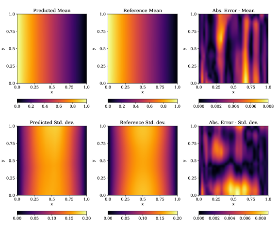
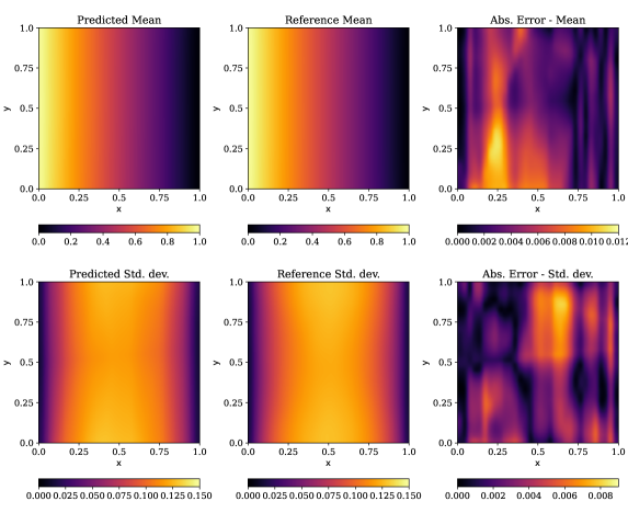
Our aim with this problem is to directly learn the map from lengthscale pair, , to the parameters of the distribution, i.e.,, of the uncertain solution for a given location , thereby propagating the uncertainty with one forward evaluation of the MD-NOMAD. The number of training epochs and the number of mixture component is equal to and respectively. Furthermore, is used as an input to the branch network and is used as augmenting input for the decoder network. Also, the train and validation data split for this example is . We assess the performance of the trained MD-NOMAD on two different test lengthscale pairs — and . The results are presented in Figure 10 and Figure 11. The reference distribution and corresponding statistics are obtained from the empirical distribution of replications. Furthermore, we also compare the performance of MD-NOMAD with deterministic NOMAD (DNOMAD) using the relative -error between the predicted statistics. The corresponding results are included in Table 1. Moreover, for DNOMAD, the statistics are estimated by using MCS and trials had to be performed, whereas the statistics and even the PDFs presented in Figure 10 were obtained with analytical computations.
| Model | ||||
|---|---|---|---|---|
| Mean | Std. dev. | Mean | Std. dev. | |
| MD-NOMAD | 0.0062 | 0.0251 | 0.0090 | 0.0455 |
| DNOMAD | 0.0108 | 0.1071 | 0.0141 | 0.1955 |


5.5 1-dimensional unsteady stochastic heat equation
The stochastic heat equation is a parabolic SPDE that provides a probabilistic framework for modeling the evolution of temperature distribution in a medium, considering both deterministic diffusive heat transfer and stochastic temperature fluctuations. For the current case, we consider a 1-dimensional stochastic heat equation, and the following equation represents it:
| (15) | ||||
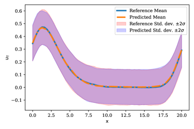
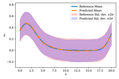
where represents the temperature at time and position , is the thermal diffusivity, is the strength of the stochastic noise, and denotes the Wiener process representing random fluctuations. The equation is solved using the pseudo-spectral method with Euler-Maruyama time integrator having a time step size inside a spatial domain up to time second. Also, periodic boundary conditions are considered, and . The experimental design is established on the stochastic noise strength , which is sampled from the uniform distribution , with and . Moreover, in this example, we are not interested in the time evolution of the state rather we are interested in the probability density for at time s or . The branch network receives input , while the decoder network’s additional input is the spatial location . The training process consists of 300 epochs, utilizing 10 mixture components. Additionally, the target solution is subjected to subsampling at a factor of 2, and corresponding input samples are accordingly preprocessed for the formation of training and validation datasets. The results that depict the performance of MD-NOMAD for the example are provided in Figure 12 and Figure 13.


5.6 1-dimensional unsteady stochastic viscous Burgers equation
As our final example, we consider the 1-dimensional stochastic viscous Burgers’ equation which is expressed as follows:
| (16) | ||||
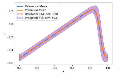
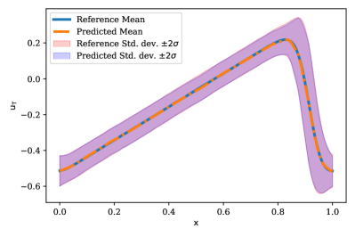
where , , and are randomly chosen fixed constants, represents the velocity at time and position , is the dynamic viscosity, is the stochastic noise strength, and denotes the Wiener process. Again, the pseudo-spectral method is used along with the Euler-Maruyama time integrator for solving the SPDE. Further, the time step size and . Moreover, even for this example, the experimental design is based on the stochastic noise strength , samples for which are drawn from the uniform distribution , with and , and the quantity of interest is the solution’s probability density at time s or . Also, the branch network takes in input , while the decoder network incorporates the spatial location as an additional input. The training process spans 300 epochs, incorporating 10 mixture components. Furthermore, the target solution is exposed to subsampling with a factor of 2. Finally, Figure 14 and Figure 15 depict the performance of MD-NOMAD for this example problem.


6 Conclusions
We introduced the mixture density-based NOMAD framework, which seamlessly integrates pointwise operator learning network NOMAD with mixture density formalism, enabling the estimation of conditional probability distributions for stochastic output functions. The components of the mixture were Gaussian distributions, which were predominantly employed for their mathematical traceability. The scalability inherited from the NOMAD architecture to handle high-dimensional problems, coupled with the ability to learn a data representation of stochastic systems, underscores the versatility and practical utility of MD-NOMAD. In our empirical assessment, we validated the efficacy of MD-NOMAD across a diverse range of stochastic ordinary and partial differential equations (including high-dimensional examples), covering both linear and nonlinear formulations, alongside analytical benchmark problems. Furthermore, the usage of MD-NOMAD was also demonstrated for one-shot uncertainty propagation in a 2-dimensional stochastic partial differential equation. In addition, as the predicted PDFs and associated statistics for MD-NOMAD can be computed analytically, without resorting to MC simulations, the proposed framework experiences an improved computational efficiency, thereby bolstering its practical applicability. However, it is important to note that MD-NOMAD necessitates additional attention to adjusting an extra hyperparameter compared to deterministic NOMAD, specifically, the number of mixture components. Presently, the determination of the number of mixture components relies on validation error. However, Bayesian decision-making can be leveraged for automatic selection of the number of mixture components in later studies. Furthermore, future investigations into alternative architectures beyond the FCN utilized in this study, along with further endeavors such as assessing the capabilities of MD-NOMAD in constructing surrogates for complex 3-dimensional problems like turbulent channel flow, would be of considerable interest.
7 Acknowledgement
SC acknowledges the financial support received from Ministry of Port and Shipping via letter no. ST-14011/74/MT (356529)
References
- [1] Christopher M Bishop. Mixture density networks. 1994.
- [2] Géraud Blatman and Bruno Sudret. Adaptive sparse polynomial chaos expansion based on least angle regression. Journal of computational Physics, 230(6):2345–2367, 2011.
- [3] Jonah Botvinick-Greenhouse, Yunan Yang, and Romit Maulik. Generative modeling of time-dependent densities via optimal transport and projection pursuit. Chaos: An Interdisciplinary Journal of Nonlinear Science, 33(10), 2023.
- [4] Thomas Browne, Bertrand Iooss, Loïc Le Gratiet, Jérôme Lonchampt, and Emmanuel Remy. Stochastic simulators based optimization by gaussian process metamodels–application to maintenance investments planning issues. Quality and Reliability Engineering International, 32(6):2067–2080, 2016.
- [5] Souvik Chakraborty et al. Deep physics corrector: A physics enhanced deep learning architecture for solving stochastic differential equations. Journal of Computational Physics, 479:112004, 2023.
- [6] Felix Dietrich, Alexei Makeev, George Kevrekidis, Nikolaos Evangelou, Tom Bertalan, Sebastian Reich, and Ioannis G Kevrekidis. Learning effective stochastic differential equations from microscopic simulations: Linking stochastic numerics to deep learning. Chaos: An Interdisciplinary Journal of Nonlinear Science, 33(2), 2023.
- [7] Sam Efromovich. Dimension reduction and adaptation in conditional density estimation. Journal of the American Statistical Association, 105(490):761–774, 2010.
- [8] Jianqing Fan and Irene Gijbels. Local polynomial modelling and its applications: monographs on statistics and applied probability 66. Routledge, 2018.
- [9] Shailesh Garg and Souvik Chakraborty. Variational bayes deep operator network: a data-driven bayesian solver for parametric differential equations. arXiv preprint arXiv:2206.05655, 2022.
- [10] Peter Hall, Jeff Racine, and Qi Li. Cross-validation and the estimation of conditional probability densities. Journal of the American Statistical Association, 99(468):1015–1026, 2004.
- [11] Trevor J Hastie and Robert J Tibshirani. Generalized additive models. Routledge, 2017.
- [12] Eugene Isaacson and Herbert Bishop Keller. Analysis of numerical methods. Courier Corporation, 1994.
- [13] Patrick Kidger, James Foster, Xuechen Li, and Terry J Lyons. Neural sdes as infinite-dimensional gans. In International conference on machine learning, pages 5453–5463. PMLR, 2021.
- [14] Peter E Kloeden and Eckhard Platen. Stochastic differential equations. In Numerical Solution of Stochastic Differential Equations, pages 103–160. Springer, 1992.
- [15] Nikola Kovachki, Zongyi Li, Burigede Liu, Kamyar Azizzadenesheli, Kaushik Bhattacharya, Andrew Stuart, and Anima Anandkumar. Neural operator: Learning maps between function spaces with applications to pdes. Journal of Machine Learning Research, 24(89):1–97, 2023.
- [16] Samuel Lanthaler, Siddhartha Mishra, and George E Karniadakis. Error estimates for deeponets: A deep learning framework in infinite dimensions. Transactions of Mathematics and Its Applications, 6(1):tnac001, 2022.
- [17] Randall J LeVeque. Finite volume methods for hyperbolic problems, volume 31. Cambridge university press, 2002.
- [18] Randall J LeVeque. Finite difference methods for ordinary and partial differential equations: steady-state and time-dependent problems. SIAM, 2007.
- [19] Zongyi Li, Nikola Kovachki, Kamyar Azizzadenesheli, Burigede Liu, Kaushik Bhattacharya, Andrew Stuart, and Anima Anandkumar. Fourier neural operator for parametric partial differential equations. arXiv preprint arXiv:2010.08895, 2020.
- [20] Lu Lu, Pengzhan Jin, Guofei Pang, Zhongqiang Zhang, and George Em Karniadakis. Learning nonlinear operators via deeponet based on the universal approximation theorem of operators. Nature machine intelligence, 3(3):218–229, 2021.
- [21] Yubin Lu, Romit Maulik, Ting Gao, Felix Dietrich, Ioannis G Kevrekidis, and Jinqiao Duan. Learning the temporal evolution of multivariate densities via normalizing flows. Chaos: An Interdisciplinary Journal of Nonlinear Science, 32(3), 2022.
- [22] Peter McCullagh and John A Nelder. Generalized linear models. Routledge, 2019.
- [23] Parviz Moin. Fundamentals of engineering numerical analysis. Cambridge University Press, 2010.
- [24] Allan Pinkus. N-widths in Approximation Theory, volume 7. Springer Science & Business Media, 2012.
- [25] Junuthula Narasimha Reddy. An introduction to the finite element method. New York, 27:14, 1993.
- [26] Yong Ren, Jun Zhu, Jialian Li, and Yucen Luo. Conditional generative moment-matching networks. Advances in Neural Information Processing Systems, 29:2928–2936, 2016.
- [27] Andreas Rößler. Runge–kutta methods for the strong approximation of solutions of stochastic differential equations. SIAM Journal on Numerical Analysis, 48(3):922–952, 2010.
- [28] Antti Saarinen, Marja-Leena Linne, and Olli Yli-Harja. Stochastic differential equation model for cerebellar granule cell excitability. PLoS computational biology, 4(2):e1000004, 2008.
- [29] Jacob Seidman, Georgios Kissas, Paris Perdikaris, and George J Pappas. Nomad: Nonlinear manifold decoders for operator learning. Advances in Neural Information Processing Systems, 35:5601–5613, 2022.
- [30] Rohit K Tripathy and Ilias Bilionis. Deep uq: Learning deep neural network surrogate models for high dimensional uncertainty quantification. Journal of computational physics, 375:565–588, 2018.
- [31] Tapas Tripura and Souvik Chakraborty. Wavelet neural operator: a neural operator for parametric partial differential equations. arXiv preprint arXiv:2205.02191, 2022.
- [32] A.B. Tsybakov. Introduction to Nonparametric Estimation. Springer Series in Statistics. Springer, New York, NY, 2009.
- [33] Liu Yang, Dongkun Zhang, and George Em Karniadakis. Physics-informed generative adversarial networks for stochastic differential equations. SIAM Journal on Scientific Computing, 42(1):A292–A317, 2020.
- [34] X. Zhu and B. Sudret. Emulation of stochastic simulators using generalized lambda models, 2021.
- [35] Xujia Zhu and Bruno Sudret. Replication-based emulation of the response distribution of stochastic simulators using generalized lambda distributions. International Journal for Uncertainty Quantification, 10(3), 2020.
- [36] Xujia Zhu and Bruno Sudret. Stochastic polynomial chaos expansions to emulate stochastic simulators. International Journal for Uncertainty Quantification, 13(2), 2023.