Benchmark of
deep-inelastic-scattering structure functions at $\mathcal{O}\left(\alpha_{s}^{3}\right)$

Valerio Bertone valerio.bertone@cea.fr Alexander Karlberg alexander.karlberg@cern.ch
Abstract

We present a benchmark comparison of the massless inclusive deep-inelastic-scattering (DIS) structure functions up to $\mathcal{O}(\alpha_{s}^{3})$ in perturbative QCD. The comparison is performed using the codes apfel++ and hoppet within the framework of the variable-flavour-number scheme and over a broad kinematic range relevant to the extraction of parton distribution functions. We provide results for both the single structure functions and the reduced cross sections in both neutral- and charged-current DIS. Look-up tables for future reference are included, and we also release the code used for the benchmark.

keywords:
Perturbative QCD , DIS , DGLAP
journal: European Physical Journal C

CERN-TH-2024-018

\affiliation

[1]organization=IRFU, CEA, Paris-Saclay, postcode=F-91191 ,city=Gif-sur-Yvette, country=France \affiliation[2]organization=CERN, Theoretical Physics Department, postcode=CH-1211 ,city=Geneva 23, country=Switzerland

1 Introduction

Deep inelastic scattering (DIS) is one of the best theoretically understood processes in perturbative QCD, cf. Refs. [1, 2] for a review. Most significantly, it offers unique insight into the proton structure, and to this day legacy DIS data still has a major impact on fits of parton distribution functions (PDFs) [3, 4, 5, 6, 7, 8, 9].

The inclusive DIS cross sections can be parametrised in terms of structure functions. These structure functions are inherently non-perturbative quantities, but they can be expressed as convolutions between hard perturbative coefficient functions and PDFs, where the latter encompass the non-perturbative contribution. As of today, the massless DIS coefficient functions are fully known up to $\mathcal{O}(\alpha_{s}^{3})$, allowing us to compute structure functions up to next-to-next-to-next-to-leading order (N3LO) accuracy [10, 11, 12, 13, 14, 15, 16, 17, 18, 19, 20, 21, 22, 23, 24, 25, 26].111We notice that, by convention, achieving N3LO would in principle imply computing the anomalous dimensions responsible for the energy evolution of strong coupling and PDFs to the same relative accuracy as the coefficient functions. We will address this point below. Very recently the code yadism [27], which computes DIS structure functions at this order, became available. However, their implementation was directly compared to apfel++ and therefore relies implicitly on the benchmark presented here.

In this paper, we present a comparison of the structure functions obtained using the two publicly available codes apfel++ [28, 29] and hoppet [30].222Technically speaking, the $\mathcal{O}(\alpha_{s}^{3})$ structure functions were already available in the struct-func-devel branch of hoppet as they were used in the proVBFH code [31, 32, 33, 34]. However, while performing this benchmark, some bugs were found in the $\mathcal{O}(\alpha_{s}^{3})$ neutral-current structure functions, and it is therefore fair to say that they have only been publicly available in hoppet as of the v1.3.0 release, which will be made public in a forthcoming paper [35], but is already available on the hoppet GitHub repository. As far as apfel++ is concerned, the $\mathcal{O}(\alpha_{s}^{3})$ structure functions are available in the current master branch of the GitHub repository, as well as in v4.8.0. The benchmark that we present here serves two purposes. First, it validates the correctness of the structure functions as implemented in the two programs. This is a highly non-trivial check in that, although the coefficient functions are identical in the two programs, the underlying technologies adopted by the two codes are not. Secondly, the results presented here provide a reference for any future numerical implementation of the DIS structure functions. To make the benchmark as resilient towards the future as possible, we carry out the benchmark using the same PDF initial conditions as those used in Ref. [36]. This avoids complications caused by numerical artefacts related to pre-computed interpolation grids such as those released through the LHAPDF interface [37]. Moreover, this guarantees the independence of the benchmark from the availability of a specific PDF set. The benchmark is carried out both on the single structure functions and on the reduced cross sections, which is what is often measured in experiments.

The paper is structured as follows. In Sect. 2, we review the DIS process and define the structure functions. The numerical setup of the benchmark is presented in Sect. 3. We finally present the benchmark in Sect. 4 before concluding in Sect. 5. A contains some comments on the large-$y$ behaviour of the non-singlet N3LO coefficient functions, while B presents look-up benchmark tables for all of the structure functions at NLO, NNLO, and N3LO accuracy for different values of $Q$ and for Bjorken $x_{\rm B}\in[10^{-5}:0.9]$.

2 The DIS structure functions

Let us begin by recalling the kinematics of the DIS process. This process is the inclusive scattering of a lepton $\ell$ with momentum $k_{i}$ off a proton $p$ with momentum $P$ via the exchange of a virtual electroweak gauge boson $V$ with momentum $q$ and large (negative) virtuality $Q^{2}=-q^{2}\gg\Lambda_{\rm QCD}^{2}$, where $\Lambda_{\rm QCD}$ is the typical hadronic scale. Due to the large virtuality of the vector boson, the proton breaks up leaving in the final state the scattered lepton $\ell^{\prime}$ with momentum $k_{f}=k_{i}-q$ and a remnant $X$, with respect to which we are fully inclusive:

$$\ell(k_{i})+p(P)\rightarrow V(q)\rightarrow\ell^{\prime}(k_{f})+X\,.$$ (1)

It is useful to introduce the customary DIS variables $x_{\rm B}$ (Bjorken’s variable) and $y$ (inelasticity) defined as:

$\displaystyle x_{\rm B}=\frac{Q^{2}}{2P\cdot q},\qquad y=\frac{P\cdot q}{P\cdot k_{i}}=\frac{Q^{2}}{x_{\rm B}s}\,,$ (2)

where $s=(k_{i}+P)^{2}$ is the collision center-of-mass energy squared.333We assume that incoming lepton and proton are both massless, i.e. $k_{i}^{2}=P^{2}=0$. In order to describe the interaction between the proton and the appropriate electroweak current, i.e. the neutral current (NC) mediated by a $V=\gamma/Z$ boson or the charged current (CC) mediated by a $V=W^{\pm}$ boson, it is useful to consider the hadronic tensor $W_{\mu\nu}^{V}$. The spin-averaged hadronic tensor defines the structure functions $F_{1}$, $F_{2}$, and $F_{3}$ through [38]:

$\displaystyle W^{V}_{\mu\nu}=\left(-g_{\mu\nu}+\frac{q_{\mu}q_{\nu}}{q^{2}}\right)F^{V}_{1}(x_{\rm B},Q^{2})+\frac{\hat{P}_{\mu}\hat{P}_{\nu}}{P\cdot q}F^{V}_{2}(x_{\rm B},Q^{2})-i\epsilon_{\mu\nu\alpha\beta}\frac{q^{\alpha}P^{\beta}}{2P\cdot q}F^{V}_{3}(x_{\rm B},Q^{2}),$ (3)

where:

$\displaystyle\hat{P}_{\mu}=P_{\mu}-\frac{P\cdot q}{q^{2}}q_{\mu}\,.$ (4)

It is also customary to define the longitudinal structure function as $F_{L}^{V}=F_{2}^{V}-2x_{\rm B}F_{1}^{V}$. With the structure functions at hand, we can write the NC cross section ($\ell^{\pm}p\to\ell^{\pm}+X$) as:

$$\frac{\mathrm{d}\sigma_{\mathrm{NC}}^{\pm}}{\mathrm{d}x_{\rm B}\mathrm{d}Q^{2}}=\frac{2\pi\alpha^{2}}{x_{\rm B}Q^{4}}y_{+}\left[F_{2}^{\gamma/Z}\mp\frac{y_{-}}{y_{+}}x_{\rm B}F_{3}^{\gamma/Z}-\frac{y^{2}}{y_{+}}F_{L}^{\gamma/Z}\right]\,,$$ (5)

where $y_{\pm}=1\pm(1-y)^{2}$ and $\alpha$ is the fine structure constant. Similarly, the CC cross section for ($\ell^{\pm}p\to\nu_{\ell}(\overline{\nu}_{\ell})+X$) reads:

$$\frac{\mathrm{d}\sigma_{\mathrm{CC}}^{\pm}}{\mathrm{d}x_{\rm B}\mathrm{d}Q^{2}}=\frac{\pi\alpha^{2}}{8x_{\rm B}\sin^{4}\theta_{W}}\left(\frac{1}{M_{W}^{2}+Q^{2}}\right)^{2}\left[y_{+}F_{2}^{W^{\pm}}\mp y_{-}x_{\rm B}F_{3}^{W^{\pm}}-y^{2}F_{L}^{W^{\pm}}\right],\,$$ (6)

where $M_{W}$ is the mass of the $W$ boson and $\theta_{W}$ is the electroweak mixing angle. Some experiments, such as those at the HERA collider [7], release the so-called “reduced” cross sections that are related to the standard cross sections as follows:

$$\begin{array}[]{l}\displaystyle\sigma_{\rm NC,red}^{\pm}=\left[\frac{2\pi\alpha^{2}}{x_{\rm B}Q^{4}}y_{+}\right]^{-1}\frac{\mathrm{d}\sigma_{\mathrm{NC}}^{\pm}}{\mathrm{d}x_{\rm B}\mathrm{d}Q^{2}}=F_{2}^{\gamma/Z}\mp\frac{y_{-}}{y_{+}}x_{\rm B}F_{3}^{\gamma/Z}-\frac{y^{2}}{y_{+}}F_{L}^{\gamma/Z}\,,\\ \\ \displaystyle\sigma_{\rm CC,red}^{\pm}=\left[\frac{\pi\alpha^{2}}{4\sin^{4}\theta_{W}x_{\rm B}}\left(\frac{1}{M_{W}^{2}+Q^{2}}\right)^{2}\right]^{-1}\frac{\mathrm{d}\sigma_{\mathrm{CC}}^{\pm}}{\mathrm{d}x_{\rm B}\mathrm{d}Q^{2}}=\frac{y_{+}}{2}F_{2}^{W^{\pm}}\mp\frac{y_{-}}{2}x_{\rm B}F_{3}^{W^{\pm}}-\frac{y^{2}}{2}F_{L}^{W^{\pm}}\,.\end{array}$$ (7)

The QCD collinear factorisation theorem allows us to express the structure functions as convolutions of the PDFs, $f_{a}$, with the short-distance coefficient functions, $C_{i}$:444Note that, according to the usual definitions, the overall factor $x_{\rm B}$ on the r.h.s. of Eq. (8) only applies to $F_{2}^{V}$ and $F_{L}^{V}$, while it is not present for $F_{3}^{V}$. This is the meaning of the parentheses around $x_{\rm B}$ itself and the indices $i=(2),(L)$.

$$F_{i}^{V}\equiv F_{i}^{V}(x_{\rm B},Q^{2})=(x_{\rm B})\sum_{a}\left[C_{i,a}^{V}\otimes f_{a}\right]\left(x_{\rm B},Q^{2},\mu_{\rm R}^{2},\mu_{\rm F}^{2}\right)\,,\quad i=(2),(L),3\,,$$ (8)

where the index $a$ runs over the gluon ($a=g$) and all active quark flavours and anti-flavours ($a=q,\overline{q}$) at the scale $Q^{2}$.555Specifically, if the mass $m_{q}$ of the quark flavour $q$ is such that $m_{q}^{2}<Q^{2}$, this flavour contributes to the cross section, otherwise it does not. In practice, down, up, and strange quarks always contribute in that their masses are always far below the typical hard scale $Q^{2}$ where factorisation applies. For this reason they are called light quarks. Conversely, charm, bottom, and possibly top quarks get activated at the respective mass scales, therefore they are referred to as heavy quarks. This is a possible implementation of the of the so-called decoupling theorem [39] that goes under the name of zero-mass variable-flavour-number scheme (ZM-VFNS). According to this theorem, for $m_{q}^{2}\ll Q^{2}$ the quark flavour $q$ must drop from the calculation. The ZM-VFNS enforces this constraint already when $m_{q}^{2}<Q^{2}$, which effectively amounts to neglecting positive powers of the ratio $m_{q}^{2}/Q^{2}$. The Mellin-convolution symbol $\otimes$ implies one of the following equivalent integrals:

$$\begin{array}[]{rcl}\displaystyle\left[C_{i,a}^{V}\otimes f_{a}\right]\left(x_{\rm B},Q^{2},\mu_{\rm R}^{2},\mu_{\rm F}^{2}\right)&=&\displaystyle\int_{0}^{1}dy\int_{0}^{1}dz\,\delta(x_{\rm B}-yz)C_{i,a}^{V}\left(y,\alpha_{s}(\mu_{\rm R}),\frac{\mu_{\rm R}^{2}}{Q^{2}},\frac{\mu_{\rm F}^{2}}{Q^{2}}\right)f_{a}(z,\mu_{\rm F})\\ \\ &=&\displaystyle\int_{x_{\rm B}}^{1}\frac{dy}{y}C_{i,a}^{V}\left(y,\alpha_{s}(\mu_{\rm R}),\frac{\mu_{\rm R}^{2}}{Q^{2}},\frac{\mu_{\rm F}^{2}}{Q^{2}}\right)f_{a}\left(\frac{x_{\rm B}}{y},\mu_{\rm F}\right)\\ \\ &=&\displaystyle\int_{x_{\rm B}}^{1}\frac{dz}{z}C_{i,a}^{V}\left(\frac{x_{\rm B}}{z},\alpha_{s}(\mu_{\rm R}),\frac{\mu_{\rm R}^{2}}{Q^{2}},\frac{\mu_{\rm F}^{2}}{Q^{2}}\right)f_{a}(z,\mu_{\rm F})\,.\end{array}$$ (9)

2.1 Renormalisation and factorisation scale dependence

In this section, we derive the explicit dependence of the coefficient functions on the arbitrary renormalisation and factorisation scales $\mu_{\rm R}$ and $\mu_{\rm F}$, respectively. The coefficient function $C_{i,a}^{V}$ is an explicit function of the strong coupling $\alpha_{s}(\mu_{\rm R})$ that admits the perturbative expansion:

$$C_{i,a}^{V}\left(y,\alpha_{s}(\mu_{\rm R}),\frac{\mu_{\rm R}^{2}}{Q^{2}},\frac{\mu_{\rm F}^{2}}{Q^{2}}\right)=\sum_{n=0}^{\infty}\left(\frac{\alpha_{s}(\mu_{\rm R})}{4\pi}\right)^{n}C_{i,a}^{V,[n]}\left(y,\frac{\mu_{\rm R}^{2}}{Q^{2}},\frac{\mu_{\rm F}^{2}}{Q^{2}}\right)\,.$$ (10)

Under the assumption $\alpha_{s}(\mu_{\rm R})\ll 1$, the sum on the r.h.s. can be truncated to order $k$ to obtain a NkLO approximation of the structure functions.666If $i=L$, i.e. in the case of the longitudinal structure function, the contribution $k=0$ to the series on the r.h.s. of Eq. (10) is identically zero. Therefore, in the case of $F_{L}$ a strictly NkLO requires truncating that series at $n=k+1$. This is a consequence of the Callan-Gross relation [40], $F_{2}^{V}=2x_{\rm B}F_{1}^{V}$, valid in the parton model for spin-1/2 particles, that implies that $F_{L}^{V}=0$ at $\mathcal{O}(\alpha_{s}^{0})$. $C_{i,a}^{V}$ also depends on the ratios $\mu_{\rm R}^{2}/Q^{2}$ and $\mu_{\rm F}^{2}/Q^{2}$. Despite that the scales $\mu_{\rm R}$ and $\mu_{\rm F}$ are in principle arbitrary, in a fixed-order calculation where the series in Eq. (10) includes a finite number of terms, the presence of logarithms of these ratios requires these scales to be of order $Q=\sqrt{Q^{2}}$. In this way, the ratios $\mu_{\rm R}^{2}/Q^{2}$ and $\mu_{\rm F}^{2}/Q^{2}$ are both of order one and do not compromise the convergence of the perturbative series. Variations of $\mu_{\rm R}$ and $\mu_{\rm F}$ around $Q$ by a modest factor, typically of two, are often used as a proxy to estimate the possible impact of unknown higher-order corrections. This is due to the fact that any variation of $\mu_{\rm R}$ and $\mu_{\rm F}$ is compensated order by order in $\alpha_{s}$ by the evolution of strong coupling and PDFs, that in turn obey their own renormalisation group equations (RGEs):

$$\begin{array}[]{rcl}\displaystyle\frac{d\ln\alpha_{s}(\mu_{\rm R})}{d\ln\mu_{\rm R}^{2}}&=&\displaystyle\beta(\alpha_{s}(\mu_{\rm R}^{2}))=-\sum_{n=0}^{\infty}\left(\frac{\alpha_{s}(\mu_{\rm R})}{4\pi}\right)^{n+1}\beta_{n}\,,\\ \\ \displaystyle\frac{df_{a}(x,\mu_{\rm F})}{d\ln\mu_{\rm F}^{2}}&=&\displaystyle\sum_{b}[P_{ab}\otimes f_{b}](x,\mu_{\rm F})=\sum_{b}\sum_{n=0}^{\infty}\left(\frac{\alpha_{s}(\mu_{\rm F})}{4\pi}\right)^{n+1}[P_{ab}^{[n]}\otimes f_{b}](x,\mu_{\rm F})\,.\\ \end{array}$$ (11)

The RGEs for PDFs are usually referred to as DGLAP equations [41, 42, 43, 44] and the kernels $P_{ab}$ are called splitting functions. Given the appropriate set of boundary conditions, the solutions of these RGEs determine the evolution (or running) of both $\alpha_{s}$ and $f_{a}$ to any scale. Similarly to the DIS coefficient functions, the anomalous dimensions $\beta$ and $P_{ab}$ are expandable in powers of $\alpha_{s}$.

When computing a DIS structure function at NkLO accuracy, it is customary to truncate also the perturbative expansions in Eq. (11) at the same relative order $k$. However, this is mostly a conventional procedure that is not strictly mandatory for a correct counting of the perturbative accuracy. Strictly speaking, the truncation of the expansion in Eq. (10) is responsible for the fixed-order accuracy, while the truncation of the expansions Eq. (11) defines the logarithmic accuracy. The fixed-order accuracy counts how many corrections proportional to an integer non-negative power of $\alpha_{s}$ are included exactly in the coefficient functions. In the DIS case, the $\mathcal{O}(\alpha_{s}^{0})$ contribution gives leading-order (LO) accuracy, the inclusion of the $\mathcal{O}(\alpha_{s})$ corrections gives next-to-leading-order (NLO) accuracy, and so on. The logarithmic accuracy instead counts the number of all-order towers of logarithms of the kind $\alpha_{s}^{m}L^{n}$, with $L=\ln\left(\mu_{\rm R,F}/Q_{0}\right)$ and $Q_{0}$ the boundary-condition scale, that are being resummed by means of the evolution of $\alpha_{s}$ and PDFs.777Note that the boundary scale $Q_{0}$ can, and often is, different for $\alpha_{s}$ and PDFs. Leading-logarithmic (LL) accuracy is achieved summing all $\alpha_{s}^{n}L^{n}$ terms, next-to-leading-logarithmic (NLL) accuracy requires summing all $\alpha_{s}^{n+1}L^{n}$ terms, and so on. It is worth noting that the distinction between fixed-order and logarithmic counting is effective only when $\alpha_{s}L\sim 1$, i.e. when $L$ is large enough to compensate for the assumed smallness of $\alpha_{s}$. This holds when $\mu_{\rm R,F}\gg Q_{0}$ (or $\mu_{\rm R,F}\ll Q_{0}$), which is often the case in phenomenological applications.

Although fixed-order and logarithmic accuracies have two different origins, they are not entirely unrelated. Indeed, loosely speaking, the summation of logarithms also contributes to the fixed-order counting; for instance the term $\alpha_{s}L$, which belongs to the LL tower, can also be regarded as a NLO contribution to the DIS structure functions. Therefore, NLO accuracy must come with at least LL resummation. In general, NkLO accuracy for the DIS coefficient functions requires a minimal resummation accuracy of Nk-1LL. However, it is not incorrect to match NkLO coefficient functions to NkLL $\alpha_{s}$ and PDF resummation: this is what conventional NkLO accuracy for structure functions prescribes.

In the following, we will adopt the “conventional” counting for the computation of the DIS structure functions up to NNLO, i.e. we will match NkLO coefficient functions to NkLL resummation, with $k=0,1,2$. At N3LO, we will instead use the “minimal” prescription and match N3LO coefficient functions to NNLL resummation. The reason for this choice is that, as of today, splitting functions are fully known only up to $\mathcal{O}(\alpha_{s}^{3})$ [45, 46, 47, 48, 49, 50, 51, 52, 53, 54, 17, 18, 25]. Accompanied by the $\mathcal{O}(\alpha_{s}^{3})$ corrections to the $\beta$-function in Eq. (11[55, 56, 57, 58, 59] and the mass threshold corrections to both the running coupling and the parton distributions [60, 61, 62], this allows us to achieve plain NNLL resummation. While the $\mathcal{O}(\alpha_{s}^{4})$ corrections to the $\beta$-function are known [63, 64], this is not the case for the splitting functions, which prevents attaining exact N3LL resummation, in spite of the recent significant progress made in determining them at this order [65, 66, 67, 68, 69, 70, 71, 72]. In contrast, all mass threshold corrections to the running coupling [60] and the parton distributions are known at this order [73, 74, 75, 76, 77, 78, 79, 80, 81, 82].

It is also worth mentioning that, in order to compute the single ingredients of the factorisation formula for the structure functions on the r.h.s. of Eq. (8), it is necessary to specify a renormalisation/factorisation scheme. While the dependence on the scheme cancels out order by order in $\alpha_{s}$, it determines the specific form of the coefficient functions and of the anomalous dimensions ($\beta$-function and splitting functions). Throughout this work, we will use the modified minimal-subtraction ($\overline{\mbox{MS}}$) scheme.

The evolution equations in Eq. (11) allow us to determine the dependence on $\mu_{\rm R}$ and $\mu_{\rm F}$ of the perturbative coefficients $C_{i,a}^{V,[n]}$ in Eq. (10). Indeed, provided that $\mu_{\rm R,F}\simeq Q$, one can perturbatively solve the RGEs in Eq. (11) to evolve $\alpha_{s}$ and PDFs from the scales $\mu_{\rm R}$ and $\mu_{\rm F}$, respectively, to the scale $Q$ [83, 15, 84], obtaining:

$$\frac{\alpha_{s}(Q)}{4\pi}=\frac{\alpha_{s}({\mu_{\mathrm{R}}})}{4\pi}+\left(\frac{\alpha_{s}({\mu_{\mathrm{R}}})}{4\pi}\right)^{2}L_{R}\beta_{0}+\left(\frac{\alpha_{s}({\mu_{\mathrm{R}}})}{4\pi}\right)^{3}(L_{R}^{2}\beta_{0}^{2}+L_{R}\beta_{1})+\mathcal{O}(\alpha_{s}^{4})\,,$$ (12)

and:

$$\begin{array}[]{rcl}f_{a}(x,Q)&=&\displaystyle f_{a}(x,{\mu_{\mathrm{F}}})-L_{F}\Bigg{\{}\left(\frac{\alpha_{s}({\mu_{\mathrm{R}}})}{4\pi}\right)P_{ab}^{[0]}\\ \\ &+&\displaystyle\left(\frac{\alpha_{s}({\mu_{\mathrm{R}}})}{4\pi}\right)^{2}\Bigg{[}P_{ab}^{[1]}-\frac{1}{2}L_{F}P_{ac}^{[0]}\otimes P_{cb}^{[0]}-\left(\frac{L_{F}}{2}-L_{R}\right)\beta_{0}P_{ab}^{[0]}\Bigg{]}\\ \\ &+&\displaystyle\left(\frac{\alpha_{s}({\mu_{\mathrm{R}}})}{4\pi}\right)^{3}\Bigg{[}P_{ab}^{[2]}-\frac{1}{2}L_{F}\left(P_{ac}^{[0]}\otimes P_{cb}^{[1]}+P_{ac}^{[1]}\otimes P_{cb}^{[0]}\right)+\frac{1}{6}L_{F}^{2}P_{ac}^{[0]}\otimes P_{cd}^{[0]}\otimes P_{db}^{[0]}\\ \\ &+&\displaystyle\left(\frac{L_{F}}{2}-L_{R}\right)\beta_{0}\left(L_{F}P_{ac}^{[0]}\otimes P_{cb}^{[0]}-2P_{ab}^{[1]}\right)+\left(L_{R}^{2}-L_{F}L_{R}+\frac{1}{3}L_{F}^{2}\right)\beta_{0}^{2}P_{ab}^{[0]}\\ \\ &-&\displaystyle\left(\frac{L_{F}}{2}-L_{R}\right)\beta_{1}P_{ab}^{[0]}\Bigg{]}\Bigg{\}}\otimes f_{b}(x,{\mu_{\mathrm{F}}})+\mathcal{O}(\alpha_{s}^{4})\,,\end{array}$$ (13)

where a summation over repeated indices is understood and we introduced the shorthand notation:

$$L_{R}=\ln\left(\frac{\mu_{\rm R}^{2}}{Q^{2}}\right)\,,\quad L_{F}=\ln\left(\frac{\mu_{\rm F}^{2}}{Q^{2}}\right)\,.$$ (14)

With these equalities at hand, one can solve iteratively order by order in $\alpha_{s}$ the following equality:

$$\sum_{a}\left[C_{i,a}^{V}\otimes f_{a}\right]\left(x_{\rm B},Q^{2},\mu_{\rm R}^{2},\mu_{\rm F}^{2}\right)=\sum_{a}\left[C_{i,a}^{V}\otimes f_{a}\right]\left(x_{\rm B},Q^{2},Q^{2},Q^{2}\right)\,,$$ (15)

which immediately implies:

$$\small\begin{array}[]{rcl}\displaystyle C_{i,a}^{V,[0]}\left(y,\frac{\mu_{\rm R}^{2}}{Q^{2}},\frac{\mu_{\rm F}^{2}}{Q^{2}}\right)&=&\displaystyle c_{i,a}^{V,[0]}(y)\,,\\ \\ \displaystyle C_{i,a}^{V,[1]}\left(y,\frac{\mu_{\rm R}^{2}}{Q^{2}},\frac{\mu_{\rm F}^{2}}{Q^{2}}\right)&=&\displaystyle c_{i,a}^{V,[1]}(y)-L_{F}\left[c_{i,b}^{V,[0]}\otimes P_{ba}^{[0]}\right](y)\,,\\ \\ \displaystyle C_{i,a}^{V,[2]}\left(y,\frac{\mu_{\rm R}^{2}}{Q^{2}},\frac{\mu_{\rm F}^{2}}{Q^{2}}\right)&=&\displaystyle c_{i,a}^{V,[2]}(y)+L_{R}\beta_{0}c_{i,a}^{V,[1]}(y)-L_{F}\left[c_{i,b}^{V,[1]}\otimes P_{ba}^{[0]}\right](y)\\ \\ &+&\displaystyle L_{F}c_{i,b}^{V,[0]}\otimes\left[\left(\frac{L_{F}}{2}-L_{R}\right)\beta_{0}P_{ba}^{[0]}+\frac{1}{2}L_{F}P_{bc}^{[0]}\otimes P_{ca}^{[0]}-P_{ba}^{[1]}\right](y)\,,\\ \\ \displaystyle C_{i,a}^{V,[3]}\left(y,\frac{\mu_{\rm R}^{2}}{Q^{2}},\frac{\mu_{\rm F}^{2}}{Q^{2}}\right)&=&\displaystyle c_{i,a}^{V,[3]}(y)+2L_{R}\beta_{0}c_{i,a}^{V,[2]}(y)-L_{F}\left[c_{i,b}^{V,[2]}\otimes P_{ba}^{[0]}\right](y)+\left(L_{R}^{2}\beta_{0}^{2}+L_{R}\beta_{1}\right)c_{i,a}^{V,[1]}(y)\\ \\ &+&\displaystyle L_{F}c_{i,b}^{V,[1]}\otimes\left[\left(\frac{L_{F}}{2}-2L_{R}\right)\beta_{0}P_{ba}^{[0]}+\frac{L_{F}}{2}P_{bc}^{[0]}\otimes P_{ca}^{[0]}-P_{ba}^{[1]}\right](y)\\ \\ &+&\displaystyle L_{F}c_{i,b}^{V,[0]}\otimes\par\bigg{[}-\beta_{0}^{2}P_{ba}^{[0]}\left(\frac{L_{F}^{2}}{3}-L_{F}L_{R}+L_{R}^{2}\right)\\ \\ &-&\displaystyle\left(\frac{L_{F}}{2}-L_{R}\right)\beta_{0}(L_{F}P_{bc}^{[0]}\otimes P_{ca}^{[0]}-2P_{ba}^{[1]})-\frac{L_{F}^{2}}{6}P_{bc}^{[0]}\otimes P_{cd}^{[0]}\otimes P_{da}^{[0]}\\ \\ &+&\displaystyle\frac{L_{F}}{2}(P_{bc}^{[0]}\otimes P_{ca}^{[1]}+P_{bc}^{[1]}\otimes P_{ca}^{[0]})-P_{ba}^{[2]}\bigg{]}(y)\,,\end{array}$$ (16)

where we have defined:

$$c_{i,a}^{V,[n]}(y)=C_{i,a}^{V,[n]}\left(y,1,1\right)\,.$$ (17)

Eq. (16) allows us to compute the structure functions up to N3LO accuracy for any choice of renormalisation and factorisation scales.

2.2 Characteristics of the structure functions

We now move to characterising the structure functions. In the NC case, structure functions have the following structure:

$$\begin{array}[]{l}\displaystyle F_{i}^{\gamma/Z}=x_{\rm B}\sum_{a}B_{a}\left[C_{i,\rm NS}^{+}\otimes f_{a}^{+}+C_{i,\rm PS}\otimes f_{\rm PS}+C_{i,g}\otimes f_{g}\right]\,,\quad i=2,L\,,\\ \\ \displaystyle F_{3}^{\gamma/Z}=\sum_{a}D_{a}\left[C_{3,\rm NS}^{-}\otimes f_{a}^{-}+C_{3,\rm PV}\otimes f_{\rm PV}\right]\,,\end{array}$$ (18)

where we have defined the following combinations of quark PDFs:

$$f_{a}^{\pm}=f_{a}\pm f_{\bar{a}}\,,\qquad f_{\text{PS}}=\sum_{a}f_{a}^{+}\,,\qquad f_{\text{PV}}=\sum_{a}f_{a}^{-}\,.$$ (19)

Importantly, in the decomposition in Eq. (18) the coefficient functions are independent of the flavour index $a$. Conversely, the electroweak charges $B_{a}$ and $D_{a}$ do depend on the flavour index as follows:

$$\begin{array}[]{l}\displaystyle B_{a}=e_{a}^{2}-2e_{a}V_{\ell}V_{a}P_{Z}+(V_{\ell}^{2}+A_{\ell}^{2})(V_{a}^{2}+A_{a}^{2})P_{Z}^{2}\,,\\ \\ \displaystyle D_{a}=-2e_{a}A_{\ell}A_{a}P_{Z}+4V_{\ell}A_{\ell}V_{a}A_{a}P_{Z}^{2}\,,\end{array}$$ (20)

where:

$$P_{Z}=\frac{1}{4\sin^{2}\theta_{W}\cos^{2}\theta_{W}}\left(\frac{Q^{2}}{Q^{2}+M_{Z}^{2}}\right)\,,$$ (21)

and $\ell$ is the lepton off which the proton scatters. The electric, vector, and axial charges for quarks and leptons are given in the Tab. 1.

$f$ $e_{f}$ $V_{f}$ $A_{f}$
$d$, $s$, $b$ $-\frac{1}{3}$ $-\frac{1}{2}+\frac{2}{3}\sin^{2}\theta_{W}$ $-\frac{1}{2}$
$u$, $c$, $t$ $+\frac{2}{3}$ $+\frac{1}{2}-\frac{4}{3}\sin^{2}\theta_{W}$ $+\frac{1}{2}$
$e$, $\mu$, $\tau$ $-1$ $-\frac{1}{2}+2\sin^{2}\theta_{W}$ $-\frac{1}{2}$
$\nu_{e}$, $\nu_{\mu}$, $\nu_{\tau}$ 00 $+\frac{1}{2}$ $+\frac{1}{2}$
Table 1: Electric, vector, and axial couplings for up-type, down-type, charged leptons, and neutrinos.

We now move to the CC structure functions whose factorised expression reads:

$$\begin{array}[]{l}\displaystyle F_{i}^{W^{\pm}}=\frac{1}{2}x_{\rm B}\left[\mp C_{i,\rm NS}^{-}\otimes\delta f_{\rm PV}+(C_{i,\rm NS}+C_{i,\rm PS})\otimes f_{\rm PS}+C_{i,g}\otimes f_{g}\right]\,,\quad i=2,L\,,\\ \\ \displaystyle F_{3}^{W^{\pm}}=\frac{1}{2}\left[\pm C_{3,\rm NS}^{+}\otimes\delta f_{\rm PS}+C_{3,\rm PV}\otimes f_{\rm PV}\right]\,,\end{array}$$ (22)

where we have defined the additional quark-PDF combinations:

$$\delta f_{\rm PS}=\sum_{a\in u\text{-type}}f_{a}^{+}-\sum_{a\in d-\text{type}}f_{a}^{+}\,,\qquad\delta f_{\rm PV}=\sum_{a\in u\text{-type}}f_{a}^{-}-\sum_{a\in d-\text{type}}f_{a}^{-}\,.$$ (23)

We notice that the expressions in Eq. (22) have been obtained under the assumption of a CKM matrix equal to the $3\times 3$ unity,888In fact, relying on unitarity, Eq. (22) is exactly true for any CKM matrix if $n_{f}=6$. which we will also use in the numerical results presented below. The corresponding expressions for a generic CKM matrix are considerably more complicated and we do not present them here.

3 Numerical setup

For our benchmark, rather than relying on a set of tabulated PDFs as for example delivered by LHAPDF [37], we decided to use a set of realistic initial-scale conditions having a simple analytic form and to carry out the evolution ourselves. Besides the obvious advantage of having full numerical control on our results, we believe that this choice will allow for easier comparison to our benchmark results. To this purpose, we selected as initial conditions for the evolution the parameterisation of Sect. 1.3 of Ref. [36]. Specifically, we chose $Q_{0}=\sqrt{2}\,\mathrm{GeV}$ as an initial scale with $\alpha_{s}(Q_{0})=0.35$. At the initial scale $Q_{0}$, only gluon and up, down, and strange quark PDFs are present while charm, bottom, and top quark PDFs are assumed to be identically zero and have their production thresholds at $m_{c}=(\sqrt{2}+\epsilon)$ GeV,999The presence of the infinitesimal parameter $\epsilon$ in $m_{c}$ is meant to ensure that $Q_{0}<m_{c}$ such that the initial conditions for both PDFs and $\alpha_{s}$ are given with $n_{f}=3$ active flavours. In practice, we take $\epsilon=10^{-9}.$ $m_{b}=4.5$ GeV, and $m_{t}=175$ GeV, respectively. At the initial scale $Q_{0}$, the PDFs are given by:

$\displaystyle xu_{v}(x,Q_{0})$ $\displaystyle=5.107200\,x^{0.8}(1-x)^{3}\,,$ (24a)
$\displaystyle xd_{v}(x,Q_{0})$ $\displaystyle=3.064320\,x^{0.8}(1-x)^{4}\,,$ (24b)
$\displaystyle x\bar{d}(x,Q_{0})$ $\displaystyle=0.1939875\,x^{-0.1}(1-x)^{6}\,,$ (24c)
$\displaystyle x\bar{u}(x,Q_{0})$ $\displaystyle=x\bar{d}(x)(1-x)\,,$ (24d)
$\displaystyle xs(x,Q_{0})$ $\displaystyle=x\bar{s}(x,Q_{0})=0.2\,(x\bar{d}(x,Q_{0})+x\bar{u}(x,Q_{0}))\,,$ (24e)
$\displaystyle xg(x,Q_{0})$ $\displaystyle=1.7\,x^{-0.1}(1-x)^{5}\,,$ (24f)

where the valence distributions are defined as $u_{v}\equiv u-\bar{u}$ and $d_{v}\equiv d-\bar{d}$. We carry out the evolution in the variable-flavour-number scheme, that is by including quark-mass thresholds in both coupling and the PDF evolutions. The resulting set of evolved PDFs both from apfel++ and hoppet are in perfect agreement with the tables in Ref. [36] at all perturbative orders.

Starting from NNLO accuracy, both splitting functions and coefficient functions become analytically very convoluted and it is customary to resort to the parameterisations provided by Moch, Vermaseren and Vogt [14, 15, 16, 17, 18, 19, 20, 21, 22, 23, 24]. These parameterisations are expected to agree with their exact counterparts at the level of $10^{-4}$ relative accuracy. In this benchmark, we thus employ exact splitting and coefficient functions up to NLO, while we use the parameterisations beyond.101010We notice that the exact expressions are available at all orders in hoppet, as discussed in A. For the PDF mass threshold corrections we use the exact expressions at all orders. In A, we comment on the differences between exact and parametrised coefficient functions.

Finally, we point out that the NC structure functions also depend on the weak mixing angle (see Sect. 2.2). In this benchmark, we employ the leading-order relation $\sin^{2}\theta_{W}=1-\frac{M_{W}^{2}}{M_{Z}^{2}}$ to compute it, using $M_{W}=80.377$ GeV and $M_{Z}=91.1876$ GeV for the mass values of $W$ and $Z$ bosons, respectively.

4 Benchmark results

In this section, we present the results of the benchmark between apfel++ and hoppet. Here, we will assess the level of agreement between the two codes at N3LO accuracy by means of a set of plots. The excellent agreement found at this order (see below) immediately implies that the agreement at lower orders is at least as good. In this section, we also take the chance to discuss the impact of scale variations on DIS structure functions at the available perturbative orders, as well as the degree of perturbative convergence moving from LO to N3LO. In B, instead, we provide look-up tables with predictions at all available perturbative orders over a broad kinematic range and for all of the DIS structure functions. We point out that apfel++ and hoppet are in exact agreement within the digits shown in those tables. Therefore, they can be used as a reference for future numerical implementations of the DIS structure functions. We also release the code used to produce them (see B for details).

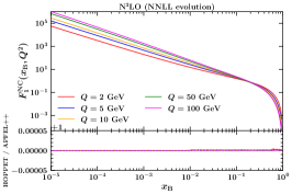
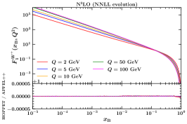
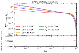
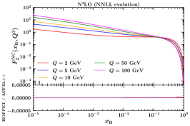
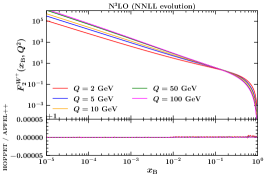
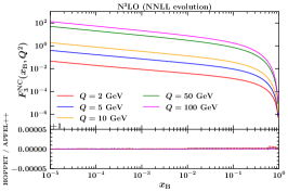
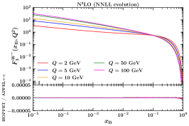
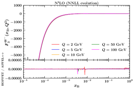
In Fig. 1, we show all structure functions both in the NC and in the CC channels at N3LO over a wide kinematic range in $x_{\rm B}$ and $Q$. Here, we set $\mu_{\rm R}=\mu_{\rm F}=Q$. While the upper panel of each plot displays the absolute values of the structure functions, the lower panel shows the ratio between apfel++ and hoppet. It is evident that the agreement between the two codes is excellent all across the board. Specifically, we observe that the relative accuracy is well below $10^{-5}$ everywhere, except for $F_{3}^{W^{-}}$ at around $x_{\rm B}\sim 3\cdot 10^{-3}-10^{-2}$. However, this slight degradation in relative accuracy is due to the fact that $F_{3}^{W^{-}}$ changes sign in that region.

Refer to caption
Refer to caption
Refer to caption
Refer to caption
Refer to caption
Refer to caption
Refer to caption
Refer to caption
Refer to caption
Figure 1: The structure functions $F_{1}$ (top row), $F_{2}$ (middle row), and $F_{3}$ (bottom row) for NC (left column), positive CC (middle column), and negative CC (right column) at N3LO as functions of $x_{\rm B}$ spanning between $10^{-5}$ and $0.9$ and for various values of the energy $Q$. The lower panels show the ratio between apfel++ and hoppet.

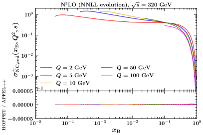
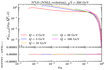
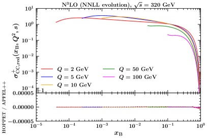
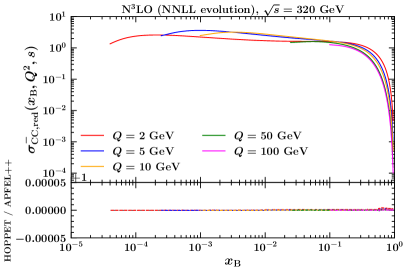
As discussed in Sect. 2, it is also relevant to consider the DIS reduced cross sections defined in Eq. (7). As a matter of fact, the HERA collider has delivered measurements for these observables [7] that are currently being employed in most of the modern PDF determinations [6, 5, 4]. In Fig. 2, we show N3LO predictions for NC (top row) and CC (bottom row) reduced cross sections relevant to $e^{+}p$ (left column) and $e^{-}p$ (right column) collisions. The centre-of-mass energy is set to $\sqrt{s}=320$ GeV, close to that of the latest runs of HERA. A broad kinematic range in $x_{\rm B}$ and $Q$ is covered and again we set $\mu_{\rm R}=\mu_{\rm F}=Q$. We notice that the curves, presented as functions of $x_{\rm B}$ for different values of $Q$, are limited in $x_{\rm B}$ by the physical requirement on the inelasticity $y\leq 1$ (see Eq. (2)). As above, the lower panel of each plot shows the ratio between predictions obtained with apfel++ and hoppet. As expected from the results presented in Fig. 1, the two codes agree well within $10^{-5}$ relative accuracy over the full kinematic range also for the reduced cross sections.

Refer to caption
Refer to caption
Refer to caption
Refer to caption
Figure 2: The reduced cross sections $\sigma_{\rm NC,red}^{+}$ (top left), $\sigma_{\rm NC,red}^{-}$ (top right), $\sigma_{\rm CC,red}^{+}$ (bottom left) and $\sigma_{\rm NC,red}^{-}$ (bottom right) at N3LO as functions of $x_{\rm B}$ spanning between $10^{-5}$ and $0.9$ and for various values of the energy $Q$. The centre-of-mass energy is set to $\sqrt{s}=320$ GeV. The lower panels show the ratio between apfel++ and hoppet.

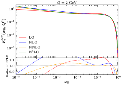
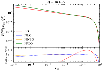
Having at our disposal four consecutive perturbative orders, it is interesting to study how well the QCD perturbative series converges in the case of inclusive DIS structure functions. In Fig. 3, we display $F_{2}^{\rm NC}$ as a function of $x_{\rm B}$ at $Q=2$ GeV (left) and $Q=10$ GeV (right) computed with $\mu_{\rm R}=\mu_{\rm F}=Q$. Each plot shows this structure function for all perturbative orders between LO and N3LO, with the lower panel giving the ratio to N3LO. The pattern is somewhat the expected one. At $Q=2$ GeV, due to the relatively large value of $\alpha_{s}$, the convergence is slower with differences between NNLO and N3LO that can exceed 10%, particularly at small and large values of $x_{\rm B}$. At $Q=10$ GeV, instead, the convergence is much faster with NNLO and N3LO very close to each other everywhere, except for very large values of $x_{\rm B}$.

Refer to caption
Refer to caption
Figure 3: The structure function $F_{2}^{\rm NC}$ plotted as a function of $x_{\rm B}$ in the range $[10^{-5}:0.9]$ at $Q=2$ GeV (left) and $Q=10$ GeV (right). Each plot displays the curves at LO, NLO, NNLO, and N3LO with the lower panel showing the ratio to N3LO.

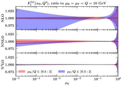
The perturbative convergence can also be studied by looking at how renormalisation and factorisation scale variations behave. In Sect. 2, we provided all relevant expressions to perform these variations up to N3LO accuracy. We point out that we have checked that apfel++ and hoppet agree within the same level of accuracy discussed above also when scales are varied. In Fig. 4, we show the effect of varying the renormalisation scale $\mu_{\rm R}$ (red bands) and the factorisation scale $\mu_{\rm F}$ (blue bands) by a factor of $2$ up and down with respect to $Q$ relative to the central-scale choice $\mu_{\rm R}=\mu_{\rm F}=Q$. The left plot has been obtained with $Q=2$ GeV while the right plot with $Q=10$ GeV. In each of them the top panel shows variations at NLO, the central panel at NNLO, and the bottom panel at N3LO. We did not include the LO panel because at this order inclusive DIS structure functions are independent of $\mu_{\rm R}$ while $\mu_{\rm F}$ gives rise to very large bands.111111We notice that the bands shown in Fig. 4 represent the area enclosed between the curves obtained with $\mu_{\rm R,F}/Q=1/2$ and $\mu_{\rm R,F}/Q=2$. It often happens that scale variations are not monotonic, such that the central-scale curve $\mu_{\rm R,F}/Q=1$ falls outside the bands. In order to give a more reliable estimate of the perturbative uncertainty related to missing higher-order corrections, one should perform a scan between $\mu_{\rm R,F}/Q=1/2$ and $\mu_{\rm R,F}/Q=2$ and quote the envelope as an uncertainty. However, here we do not mean to provide a realistic estimate of the scale uncertainties but we only want to study the perturbative convergence. Therefore, we limit to consider $\mu_{\rm R,F}/Q=1/2$ and $\mu_{\rm R,F}/Q=2$ only. As expected, scale-variation bands shrink significantly moving from NLO to N3LO at both scales. However, the reduction is much more pronounced at $Q=10$ GeV than at $Q=2$ GeV, as a consequence of the decrease in $\alpha_{s}$ value.

Refer to caption
Refer to caption
Figure 4: Relative scale variations on $F_{2}^{\rm NC}$ as functions of $x_{\rm B}$ for $Q=2$ GeV (left) and $Q=10$ GeV (right). The red (blue) bands correspond to variations of $\mu_{\rm R}$ ($\mu_{\rm F}$) by a factor of $2$ up and down around $Q$. Variations are shown for NLO (upper panels), NNLO (central panels), and N3LO (lower panels).

5 Conclusion

As N3LO PDFs start to emerge, see e.g. Refs. [85, 86], it will become increasingly important to have reliable N3LO predictions for inclusive DIS cross sections available. Indeed, DIS measurements are and will likely remain one of the main sources of experimental information that enter modern determinations of PDFs. Moreover DIS is one of the very few processes for which N3LO corrections to the partonic cross sections, albeit only in the quark massless limit, are exactly known.

In this paper, we have benchmarked the implementation of the massless DIS structure functions to N3LO accuracy by comparing the predictions provided by two widely used codes: apfel++ [28, 29] and hoppet [30]. In this benchmark, we considered both NC and CC structure functions relevant to the computation of DIS cross sections respectively characterised by the exchange of a neutral ($\gamma/Z$) and a charged ($W^{\pm}$) virtual vector boson. The numerical setup closely follows that of Ref. [36]. Specifically, we used a realistic set of initial-scale PDFs that were evolved to the relevant scales before convoluting them with the appropriate DIS coefficient functions. This workflow was independently implemented in both apfel++ and hoppet before comparing the respective predictions. On top of the single structure functions, we also compared reduced cross sections as those delivered by the HERA experiments [7].

We found a relative agreement between apfel++ and hoppet at the $10^{-5}$ level or better over a very wide kinematic range in $Q\in[2:100]$ GeV and $x_{\rm B}\in[10^{-5}:0.9]$ for all structure functions and reduced cross sections. Additionally, we also investigated the perturbative convergence by comparing predictions for $F_{2}^{\rm NC}$ at all available perturbative orders, i.e. from LO to N3LO, and by estimating the effect of renormalisation and factorisation scale variations. We found the expected pattern according to which $F_{2}^{\rm NC}$ exhibits a good perturbative convergence, especially for large values of $Q$. apfel++ and hoppet were benchmarked also against scale variations.

The benchmark carried out in this paper, thanks to its high accuracy level, provides a solid reference for any future implementation of the DIS coefficient functions up to N3LO perturbative accuracy. In order to make our results fully reproducible and facilitate the comparison to future implementations, we made the code used for this benchmark available at:

https://github.com/alexanderkarlberg/n3lo-structure-function-benchmarks,

where we also provide a short documentation and the suite of Matplotlib scripts that we used to produce the plots shown in this paper.

Acknowledgments

We are grateful to Gavin Salam for many fruitful discussions and a critical reading of the paper. A. K. is also grateful to Frédéric Dreyer for the initial work on the structure functions in hoppet. V. B. is supported by the European Union Horizon 2020 research and innovation program under grant agreement Num. 824093 (STRONG-2020).

Appendix A Comments on the $y\to 1$ behaviour of the coefficient functions

In the course of this benchmark, we have encountered some minor differences between the exact N3LO coefficient functions and the parameterisations used here and given in Refs. [19, 20, 21, 23]. The differences arise for $y\gtrsim 0.9$ in the regular part of the non-singlet coefficient functions.121212Specifically, in the routines CLNP3A, C2NP3A, and C3NM3A of xclns3p.f, xc2ns3p.f, and xc3ns3p.f, respectively. Although the difference is phenomenologically negligible, it does have a small impact in precision studies like the benchmark presented here. The largest relative difference is found in the $c^{(3)}_{2,q}$ coefficient function, on which we focus our attention.

In general, a DIS coefficient function $C$ receives three different contributions:

  • 1.

    The singular piece $[C_{\rm sing}(y)]_{+}$, which is a combination of terms of the kind $\left[\frac{\ln^{i}(1-y)}{1-y}\right]_{+}$. The $+$-prescription is defined as:

    $$\int_{0}^{1}dy[C_{\rm sing}(y)]_{+}f(y)=\int_{0}^{1}dy\,C_{\rm sing}(y)[f(y)-f(1)]\,,$$ (25)

    and has the effect of regularising the otherwise non-integrable singularities at $y=1$.

  • 2.

    The regular piece $C_{\rm reg}(y)$, which in general can be very complicated but in the $y\rightarrow 1$ limit develops integrable singular terms of the kind $\ln^{i}(1-y)$.

  • 3.

    The local piece $C_{\rm loc}\delta(1-y)$, where $C_{\rm loc}$ is a numerical constant.

Although the singular piece $[C_{\rm sing}(y)]_{+}$ dominates the coefficient function for $y\rightarrow 1$, this is not the case when it is convoluted with a parton distribution as in Eq. (8), since the $+$-prescription effectively generates a factor of $1-y$. In the limit $y\rightarrow 1$, this can be seen schematically as follows:

$\displaystyle C\otimes f$ $\displaystyle=\int_{x_{\rm B}}^{1}\frac{dy}{y}\left\{C_{\mathrm{reg}}(y)+\left[C_{\mathrm{sing}}(y)\right]_{+}+C_{\rm loc}\delta(1-y)\right\}f\left(\frac{x_{\rm B}}{y}\right)$
$\displaystyle\simeq\int_{x_{\rm B}}^{1}dy\left\{C_{\mathrm{reg}}(y)f(x_{\rm B})+(1-y)C_{\mathrm{sing}}(y)\left[f(x_{\rm B})+x_{\rm B}f^{\prime}(x_{\rm B})\right]+\dots\right\}\,,$ (26)

where in the second line we have expanded $f(x_{\rm B}/y)/y$ around $y=1$ and neglected the local piece as well as the additional terms proportional to $\ln^{i+1}(1-x_{\rm B})\delta(1-y)$ generated by the $+$-prescription. Therefore, in order to achieve accurate results when parameterising $C$, it is necessary to correctly account for the large-$y$ behaviour of $C_{\rm reg}$.

The solid green curve on the l.h.s. of Fig. 5 shows the ratio between the regular part of the parametrisation for $c_{2,q}^{(3)}$ given in Eq. (4.11) of Ref. [20] and its exact counterpart as a function of $1-y$. As can be seen, the ratio increases as $1-y$ approaches zero and, in the range shown on the plot, it reaches $8\%$.

In order to investigate this difference, we considered the large-$y$ limit of the regular part of all $\mathcal{O}(\alpha_{s}^{3})$ non-singlet coefficient functions, which in this region admit the following expansion:

$\displaystyle c_{k,q,{\rm reg}}^{(3)}(y)\simeq\sum_{i=1}^{5}L_{i}^{(k)}\ln^{i}(1-y)\,,$ (27)

with $k=2,3,L$. The coefficients $L_{i}$ can be found in Refs. [20, 23]. Since these coefficients are non-trivial to derive, we recomputed them finding two minor typos in the expressions for $c^{(3)}_{L,q,{\rm reg}}$ reported in Ref. [20]. Specifically, for the coefficients of $c^{(3)}_{2,q,{\rm reg}}$ we find:

$\displaystyle L_{5}^{(2)}\!\!\!$ $\displaystyle=\!$  $\displaystyle-\>8\>\*{C^{\,3}_{F}}\,,$ (28)
$\displaystyle L_{4}^{(2)}\!\!\!$ $\displaystyle=\!$ $\displaystyle{220\over 9}\>\*{C_{A}}\*{C^{\,2}_{F}}\>+\>92\>\*{C^{\,3}_{F}}\>-\>{40\over 9}\>\*{C^{\,2}_{F}}\,\*{n_{\!f}}\,,$ (29)
$\displaystyle L_{3}^{(2)}\!\!\!$ $\displaystyle=\!$ $\displaystyle-\>{484\over 27}\>\*{C^{\,2}_{A}}\*{C_{F}}-\>{C_{A}}\*{C^{\,2}_{F}}\*\>\Bigg{[}{10976\over 27}-64\,\*{\zeta_{\>\!2}}\Bigg{]}\>-\>{C^{\,3}_{F}}\*\>[38-32\,\*{\zeta_{\>\!2}}]$ (30)
$\displaystyle\mbox{{}}\>+\>{176\over 27}\>\*{C_{A}}\*{C_{F}}\,\*{n_{\!f}}\>+\>{1832\over 27}\>\*{C^{\,2}_{F}}\,\*{n_{\!f}}\>-\>{16\over 27}\>\*{C_{F}}\,\*{n^{\,2}_{\!f}}\,,$
$\displaystyle L_{2}^{(2)}\!\!\!$ $\displaystyle=\!$ $\displaystyle{C^{\,2}_{A}}\*{C_{F}}\*\>\Bigg{[}{11408\over 27}-{266\over 3}\>\*{\zeta_{\>\!2}}-32\,\*{\zeta_{\>\!3}}\Bigg{]}\>+\>{C_{A}}\*{C^{\,2}_{F}}\*\>\Bigg{[}{11501\over 9}-292\,\*{\zeta_{\>\!2}}-160\,\*{\zeta_{\>\!3}}\Bigg{]}$ (31)
$\displaystyle\mbox{{}}-\>{C^{\,3}_{F}}\*\>\Bigg{[}{1199\over 3}+688\,\*{\zeta_{\>\!2}}+48\,\*{\zeta_{\>\!3}}\Bigg{]}\>-\>{C_{A}}\*{C_{F}}\,\*{n_{\!f}}\*\>\Bigg{[}{3694\over 27}-{64\over 3}\>\*{\zeta_{\>\!2}}\Bigg{]}$
$\displaystyle\mbox{{}}-\>{C^{\,2}_{F}}\,\*{n_{\!f}}\*\>\Bigg{[}{2006\over 9}-{16\over 3}\,\*{\zeta_{\>\!2}}\Bigg{]}\>+\>{296\over 27}\>\*{C_{F}}\,\*{n^{\,2}_{\!f}}\,,$
$\displaystyle L_{1}^{(2)}\!\!\!$ $\displaystyle=\!$ $\displaystyle-\>{C^{\,2}_{A}}\*{C_{F}}\*\>\Bigg{[}{215866\over 81}-824\>\*{\zeta_{\>\!2}}-{1696\over 3}\,\*{\zeta_{\>\!3}}+{304\over 5}\>\*{\zeta_{2}^{\,2}}\Bigg{]}\>+\>{C_{A}}\*{C^{\,2}_{F}}\*\>\Bigg{[}{126559\over 162}$ (32)
$\displaystyle+872\>\*{\zeta_{\>\!2}}+792\>\*{\zeta_{\>\!3}}-{1916\over 5}\>\*{\zeta_{2}^{\,2}}\Bigg{]}\>+\>{C^{\,3}_{F}}\*\>\Bigg{[}{157\over 6}+{1268\over 3}\>\*{\zeta_{\>\!2}}$
$\displaystyle-272\,\*{\zeta_{\>\!3}}+488\>\*{\zeta_{2}^{\,2}}\Bigg{]}\>+\>{C_{A}}\*{C_{F}}\,\*{n_{\!f}}\*\>\Bigg{[}{64580\over 81}-{1292\over 9}\,\*{\zeta_{\>\!2}}-{304\over 3}\,\*{\zeta_{\>\!3}}\Bigg{]}$
$\displaystyle\mbox{{}}\>-\>{C^{\,2}_{F}}\,\*{n_{\!f}}\*\>\Bigg{[}{4445\over 81}+208\>\*{\zeta_{\>\!2}}-{208\over 3}\>\*{\zeta_{\>\!3}}\Bigg{]}\>-\>{C_{F}}\,\*{n^{\,2}_{\!f}}\*\>\Bigg{[}{4432\over 81}-{32\over 9}\>\*{\zeta_{\>\!2}}\Bigg{]}\,,$

which agree with the results of Ref. [23]. Similarly, for the coefficients of $c^{(3)}_{3,q,{\rm reg}}$ we have:

$\displaystyle L_{5}^{(3)}\!\!\!$ $\displaystyle=\!$  $\displaystyle-\>8\>\*{C^{\,3}_{F}}\,,$ (33)
$\displaystyle L_{4}^{(3)}\!\!\!$ $\displaystyle=\!$ $\displaystyle{220\over 9}\>\*{C_{A}}\*{C^{\,2}_{F}}\>+\>84\>\*{C^{\,3}_{F}}\>-\>{40\over 9}\>\*{C^{\,2}_{F}}\,\*{n_{\!f}}\,,$ (34)
$\displaystyle L_{3}^{(3)}\!\!\!$ $\displaystyle=\!$ $\displaystyle-\>{484\over 27}\>\*{C^{\,2}_{A}}\*{C_{F}}-\>{C_{A}}\*{C^{\,2}_{F}}\*\>\Bigg{[}{9056\over 27}-32\,\*{\zeta_{\>\!2}}\Bigg{]}\>-\>{C^{\,3}_{F}}\*\>[110-96\,\*{\zeta_{\>\!2}}]$ (35)
$\displaystyle\mbox{{}}\>+\>{176\over 27}\>\*{C_{A}}\*{C_{F}}\,\*{n_{\!f}}\>+\>{1640\over 27}\>\*{C^{\,2}_{F}}\,\*{n_{\!f}}\>-\>{16\over 27}\>\*{C_{F}}\,\*{n^{\,2}_{\!f}}\,,$
$\displaystyle L_{2}^{(3)}\!\!\!$ $\displaystyle=\!$ $\displaystyle{C^{\,2}_{A}}\*{C_{F}}\*\>\Bigg{[}{7580\over 27}-{98\over 3}\>\*{\zeta_{\>\!2}}\Bigg{]}\>+\>{C_{A}}\*{C^{\,2}_{F}}\*\>\Bigg{[}{12031\over 9}-372\,\*{\zeta_{\>\!2}}-240\,\*{\zeta_{\>\!3}}\Bigg{]}$ (36)
$\displaystyle\mbox{{}}-\>{C^{\,3}_{F}}\*\>\Bigg{[}{1097\over 3}+656\,\*{\zeta_{\>\!2}}+16\,\*{\zeta_{\>\!3}}\Bigg{]}\>-\>{C_{A}}\*{C_{F}}\,\*{n_{\!f}}\*\>\Bigg{[}{2734\over 27}-{16\over 3}\>\*{\zeta_{\>\!2}}\Bigg{]}$
$\displaystyle\mbox{{}}-\>{C^{\,2}_{F}}\,\*{n_{\!f}}\*\>\Bigg{[}{2098\over 9}-{112\over 3}\,\*{\zeta_{\>\!2}}\Bigg{]}\>+\>{248\over 27}\>\*{C_{F}}\,\*{n^{\,2}_{\!f}}\,,$
$\displaystyle L_{1}^{(3)}\!\!\!$ $\displaystyle=\!$ $\displaystyle-\>{C^{\,2}_{A}}\*{C_{F}}\*\>\Bigg{[}{138598\over 81}-{4408\over 9}\>\*{\zeta_{\>\!2}}-272\,\*{\zeta_{\>\!3}}+{176\over 5}\>\*{\zeta_{2}^{\,2}}\Bigg{]}\>-\>{C_{A}}\*{C^{\,2}_{F}}\*\>\Bigg{[}{69833\over 162}$ (37)
$\displaystyle-\>{12568\over 9}\>\*{\zeta_{\>\!2}}-{1904\over 3}\>\*{\zeta_{\>\!3}}+{764\over 5}\>\*{\zeta_{2}^{\,2}}\Bigg{]}\>+\>{C^{\,3}_{F}}\*\>\Bigg{[}{1741\over 6}+{1220\over 3}\>\*{\zeta_{\>\!2}}$
$\displaystyle+480\,\*{\zeta_{\>\!3}}-{376\over 5}\>\*{\zeta_{2}^{\,2}}\Bigg{]}\>+\>{C_{A}}\*{C_{F}}\,\*{n_{\!f}}\*\>\Bigg{[}{45260\over 81}-108\,\*{\zeta_{\>\!2}}-\>16\,\*{\zeta_{\>\!3}}\Bigg{]}$
$\displaystyle\mbox{{}}\>+\>{C^{\,2}_{F}}\,\*{n_{\!f}}\*\>\Bigg{[}{9763\over 81}-{2224\over 9}\>\*{\zeta_{\>\!2}}-{112\over 3}\>\*{\zeta_{\>\!3}}\Bigg{]}\>-\>{C_{F}}\,\*{n^{\,2}_{\!f}}\*\>\Bigg{[}{3520\over 81}-{32\over 9}\>\*{\zeta_{\>\!2}}\Bigg{]}\,,$

which agree with the results in Ref. [23]. Finally, for the coefficients of $c^{(3)}_{L,q,{\rm reg}}$ we find:

$\displaystyle L_{4}^{(L)}\!$ $\displaystyle=\!$ $\displaystyle 8\>C_{F}^{\,3}\>\>,$ (38)
$\displaystyle L_{3}^{(L)}\!$ $\displaystyle=\!$ $\displaystyle C_{A}C_{F}^{\,2}\left[-\frac{640}{9}+32\>{\zeta_{\>\!2}}\right]\>+\>C_{F}^{\,3}\Big{[}72-64\>{\zeta_{\>\!2}}\Big{]}\>{\color[rgb]{0,0,1}\definecolor[named]{pgfstrokecolor}{rgb}{0,0,1}+\>\frac{64}{9}\>C_{F}^{2}{n_{\!f}}}\>\>,$ (39)
$\displaystyle L_{2}^{(L)}\!$ $\displaystyle=\!$ $\displaystyle C_{A}^{\,2}C_{F}\,\left[\frac{1276}{9}-56\>{\zeta_{\>\!2}}-32\>{\zeta_{\>\!3}}\right]\>+\>C_{A}C_{F}^{\,2}\,\left[-\frac{530}{9}+80\>{\zeta_{\>\!2}}+80\>{\zeta_{\>\!3}}\right]$ (40)
$\displaystyle\mbox{}+\>C_{F}^{\,3}\,\Big{[}-34-32\>{\zeta_{\>\!2}}-32\>{\zeta_{\>\!3}}\Big{]}\>+\>C_{A}C_{F}{n_{\!f}}\,\left[-\frac{320}{9}+16\>{\zeta_{\>\!2}}\right]$
$\displaystyle\mbox{}+\>C_{F}^{\,2}{n_{\!f}}\,\left[\frac{92}{9}-32\>{\zeta_{\>\!2}}\right]\>+\>\frac{16}{9}\>C_{F}{n^{\,2}_{\!f}}\>\>,$
$\displaystyle L_{1}^{(L)}\!$ $\displaystyle=\!$ $\displaystyle C_{A}^{\,2}C_{F}\,\left[-\frac{25756}{27}+\frac{3008}{9}\>{\zeta_{\>\!2}}+\frac{880}{3}\>{\zeta_{\>\!3}}-\frac{128}{5}\>{\zeta_{2}^{\,2}}\right]$ (41)
$\displaystyle\mbox{}+\>C_{A}C_{F}^{\,2}\,\left[\frac{32732}{27}-\frac{4720}{9}\>{\zeta_{\>\!2}}+\frac{472}{3}\>{\zeta_{\>\!3}}-\frac{1152}{5}\>{\zeta_{2}^{\,2}}\right]\>+\>C_{F}^{\,3}\,\Bigg{[}-264$
$\displaystyle\left.\mbox{}+16\>{\zeta_{\>\!2}}-752\>{\zeta_{\>\!3}}{\color[rgb]{0,0,1}\definecolor[named]{pgfstrokecolor}{rgb}{0,0,1}+\frac{2816}{5}\>{\zeta_{2}^{\,2}}}\right]\>+\>C_{A}C_{F}{n_{\!f}}\,\left[\frac{6640}{27}-\frac{320}{9}\>{\zeta_{\>\!2}}-\frac{256}{3}\>{\zeta_{\>\!3}}\right]$
$\displaystyle\mbox{}+\>C_{F}^{\,2}{n_{\!f}}\,\left[-\frac{4736}{27}+\frac{352}{9}\>{\zeta_{\>\!2}}+\frac{320}{3}\>{\zeta_{\>\!3}}\right]\>-\>\frac{304}{27}\>C_{F}{n^{\,2}_{\!f}}\>\>,$

which also agree with the expressions given in Ref. [20], except for the two terms highlighted in blue.

Refer to caption
Refer to caption
Figure 5: Left: The regular $\mathcal{O}(\alpha_{s}^{3})$ coefficient function $c^{(3)}_{2,\mathrm{q,reg}}$ as a function of $1-y$ plotted as a ratio to the exact expression. In green we show the parametrisation of Ref. [20]. The dashed lines show the large-$y$ expansion including progressively more terms. Right: The same plot but now showing $1$ minus the ratio on a log-scale to highlight the relative agreement.

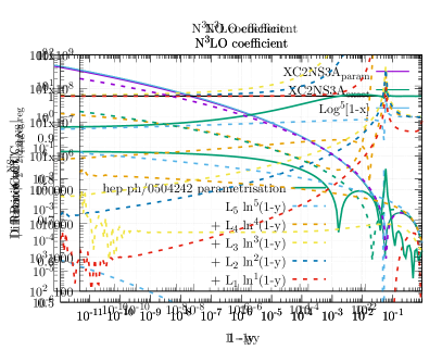
On the l.h.s. plot of Fig. 5, we also show the large-$y$ expansion of Eqs. (28)–(32) retaining progressively more terms. It can be seen that the agreement between the exact coefficient function and the large-$y$ expansion improves as $y$ increases, as expected. We conclude that the parameterisation for the regular part of $c_{2,q}^{(3)}$ reported in Eq. (4.11) of Ref. [20] does not fully account for its large-$y$ behaviour, but we also stress that the phenomenological impact is negligible.

On the r.h.s. of Fig. 5, we also show $1$ minus the ratio to the exact expression to highlight the relative agreement between the various curves. From this plot, we notice an apparent degradation of the overall precision of the exact expression as provided in Ref. [20] as $y$ approaches one (see the oscillations of the red curve).131313The Fortran implementation of this expression relies on a weight-5 extension of the hplog package [87] for the evaluation of the harmonic polylogarithms. We have explicitly checked that the decrease in precision is not due to this evaluation, as it persists also when using the HPOLY program [88]. In hoppet, where the exact expressions have been implemented, this causes some issues as the numerical convolution requires the evaluation of the coefficient functions at values of $y$ that in double precision are indistinguishable from $1$. For this reason, we switch to the large-$y$ expressions close to $y=1$.

As stated above, the difference between using exact and parametrised coefficient functions is phenomenologically negligible at the level of the structure functions. Indeed, if we reproduce the benchmark tables 510 using the exact N3LO expressions in hoppet (but keeping the parametrisations at NNLO), they typically differ from the tables obtained with the parameterised expressions only in the last (fifth) digit, and often not at all. Our benchmark program, StructureFunctionsJoint.cc, can be modified to use the exact expressions in hoppet by setting the flag param_coefs to false. Finally, we provide a Fortran file, c_ns_reg_large_x.f, with the large-$y$ expressions given above.

Appendix B Benchmark tables

In this appendix, we collect benchmark tables for all of the inclusive DIS structure functions. Results are presented for both NC and CC channels at NLO, NNLO, and N3LO accuracy, for $Q=2,50,100$ GeV, and at values of $x_{\rm B}$ ranging from $10^{-5}$ to $0.9$. Details on the numerical setup can be found in Sect. 3. The numbers reported in Tabs. 210 agree between apfel++ and hoppet within the digits shown. The code that produces the tables can be found in StructureFunctionsJoint.cc.

$x_{\rm B}$ $F_{1}^{\rm NC}$ $F_{2}^{\rm NC}$ $F_{3}^{\rm NC}$ $F_{1}^{W^{+}}$ $F_{2}^{W^{+}}$ $F_{3}^{W^{+}}$ $F_{1}^{W^{-}}$ $F_{2}^{W^{-}}$ $F_{3}^{W^{-}}$ $1.0^{-5}$ $4.9966^{+4}$ $1.5085^{+0}$ $3.4458^{-2}$ $9.6690^{+4}$ $9.6717^{+4}$ $2.8589^{+0}$ $2.8595^{+0}$ $2.1997^{+4}$ $-2.1814^{+4}$ $1.0^{-4}$ $3.5370^{+3}$ $1.0505^{+0}$ $1.7875^{-2}$ $6.8928^{+3}$ $6.9067^{+3}$ $2.0028^{+0}$ $2.0058^{+0}$ $1.7751^{+3}$ $-1.6803^{+3}$ $1.0^{-3}$ $2.4761^{+2}$ $7.1563^{-1}$ $8.7463^{-3}$ $4.8255^{+2}$ $4.8939^{+2}$ $1.3664^{+0}$ $1.3811^{+0}$ $1.5419^{+2}$ $-1.0784^{+2}$ $1.0^{-2}$ $1.8294^{+1}$ $4.9277^{-1}$ $3.9543^{-3}$ $3.3637^{+1}$ $3.6713^{+1}$ $9.0065^{-1}$ $9.6775^{-1}$ $1.7954^{+1}$ $2.9668^{+0}$ $1.0^{-1}$ $1.7795^{+0}$ $4.0072^{-1}$ $1.4381^{-3}$ $2.4287^{+0}$ $3.5994^{+0}$ $5.5218^{-1}$ $8.0596^{-1}$ $3.1699^{+0}$ $4.3670^{+0}$ $3.0^{-1}$ $5.0019^{-1}$ $3.1315^{-1}$ $5.3436^{-4}$ $4.8044^{-1}$ $1.0247^{+0}$ $3.0027^{-1}$ $6.4138^{-1}$ $8.7182^{-1}$ $1.8494^{+0}$ $5.0^{-1}$ $1.6809^{-1}$ $1.7140^{-1}$ $1.8517^{-4}$ $1.1350^{-1}$ $3.5189^{-1}$ $1.1539^{-1}$ $3.5888^{-1}$ $2.2211^{-1}$ $6.8705^{-1}$ $7.0^{-1}$ $3.7649^{-2}$ $5.3128^{-2}$ $4.0874^{-5}$ $1.5406^{-2}$ $8.0950^{-2}$ $2.1703^{-2}$ $1.1424^{-1}$ $3.0736^{-2}$ $1.6129^{-1}$ $9.0^{-1}$ $1.6475^{-3}$ $2.9702^{-3}$ $1.7405^{-6}$ $2.2898^{-4}$ $3.6497^{-3}$ $4.1266^{-4}$ $6.5798^{-3}$ $4.5806^{-4}$ $7.2985^{-3}$

Table 2: NLO stucture functions with NLL evolution at $Q=2$ GeV.

$x_{\rm B}$ $F_{1}^{\rm NC}$ $F_{2}^{\rm NC}$ $F_{3}^{\rm NC}$ $F_{1}^{W^{+}}$ $F_{2}^{W^{+}}$ $F_{3}^{W^{+}}$ $F_{1}^{W^{-}}$ $F_{2}^{W^{-}}$ $F_{3}^{W^{-}}$ $1.0^{-5}$ $6.5169^{+5}$ $1.5831^{+1}$ $3.9508^{+1}$ $1.0443^{+6}$ $1.0444^{+6}$ $2.5233^{+1}$ $2.5235^{+1}$ $2.2026^{+4}$ $-2.1598^{+4}$ $1.0^{-4}$ $3.0094^{+4}$ $7.1530^{+0}$ $1.8274^{+1}$ $4.8785^{+4}$ $4.8812^{+4}$ $1.1524^{+1}$ $1.1529^{+1}$ $1.8058^{+3}$ $-1.6079^{+3}$ $1.0^{-3}$ $1.2782^{+3}$ $2.9512^{+0}$ $7.9359^{+0}$ $2.1053^{+3}$ $2.1175^{+3}$ $4.8278^{+0}$ $4.8529^{+0}$ $1.6680^{+2}$ $-8.0951^{+1}$ $1.0^{-2}$ $5.0228^{+1}$ $1.1089^{+0}$ $3.0514^{+0}$ $8.2279^{+1}$ $8.7032^{+1}$ $1.8084^{+0}$ $1.9071^{+0}$ $2.1543^{+1}$ $1.1369^{+1}$ $1.0^{-1}$ $2.1078^{+0}$ $4.3654^{-1}$ $7.4300^{-1}$ $2.6583^{+0}$ $3.9864^{+0}$ $5.5087^{-1}$ $8.2396^{-1}$ $3.0120^{+0}$ $4.8797^{+0}$ $3.0^{-1}$ $3.3828^{-1}$ $2.0595^{-1}$ $1.6781^{-1}$ $2.8339^{-1}$ $6.6939^{-1}$ $1.7236^{-1}$ $4.0750^{-1}$ $5.0084^{-1}$ $1.2251^{+0}$ $5.0^{-1}$ $7.2949^{-2}$ $7.3507^{-2}$ $3.7503^{-2}$ $4.1693^{-2}$ $1.4855^{-1}$ $4.1970^{-2}$ $1.4969^{-1}$ $8.0977^{-2}$ $2.9141^{-1}$ $7.0^{-1}$ $9.7862^{-3}$ $1.3749^{-2}$ $4.9771^{-3}$ $3.3390^{-3}$ $2.0488^{-2}$ $4.6882^{-3}$ $2.8785^{-2}$ $6.6487^{-3}$ $4.0859^{-2}$ $9.0^{-1}$ $1.7778^{-4}$ $3.2027^{-4}$ $8.8431^{-5}$ $2.0508^{-5}$ $3.8298^{-4}$ $3.6939^{-5}$ $6.8993^{-4}$ $4.1020^{-5}$ $7.6590^{-4}$

Table 3: NLO stucture functions with NLL evolution at $Q=50$ GeV.

$x_{\rm B}$ $F_{1}^{\rm NC}$ $F_{2}^{\rm NC}$ $F_{3}^{\rm NC}$ $F_{1}^{W^{+}}$ $F_{2}^{W^{+}}$ $F_{3}^{W^{+}}$ $F_{1}^{W^{-}}$ $F_{2}^{W^{-}}$ $F_{3}^{W^{-}}$ $1.0^{-5}$ $9.9729^{+5}$ $2.3646^{+1}$ $1.0594^{+2}$ $1.3337^{+6}$ $1.3338^{+6}$ $3.1492^{+1}$ $3.1494^{+1}$ $2.1969^{+4}$ $-2.1494^{+4}$ $1.0^{-4}$ $4.3984^{+4}$ $1.0220^{+1}$ $4.8352^{+1}$ $5.9496^{+4}$ $5.9526^{+4}$ $1.3756^{+1}$ $1.3762^{+1}$ $1.8063^{+3}$ $-1.5895^{+3}$ $1.0^{-3}$ $1.7689^{+3}$ $4.0031^{+0}$ $2.0642^{+1}$ $2.4329^{+3}$ $2.4459^{+3}$ $5.4752^{+0}$ $5.5022^{+0}$ $1.6843^{+2}$ $-7.6015^{+1}$ $1.0^{-2}$ $6.4595^{+1}$ $1.4056^{+0}$ $7.7271^{+0}$ $8.8894^{+1}$ $9.3889^{+1}$ $1.9269^{+0}$ $2.0302^{+0}$ $2.1948^{+1}$ $1.2542^{+1}$ $1.0^{-1}$ $2.4151^{+0}$ $4.9778^{-1}$ $1.7757^{+0}$ $2.6188^{+0}$ $3.9463^{+0}$ $5.3990^{-1}$ $8.1189^{-1}$ $2.9482^{+0}$ $4.8573^{+0}$ $3.0^{-1}$ $3.5670^{-1}$ $2.1677^{-1}$ $3.7653^{-1}$ $2.6060^{-1}$ $6.2364^{-1}$ $1.5823^{-1}$ $3.7897^{-1}$ $4.6037^{-1}$ $1.1439^{+0}$ $5.0^{-1}$ $7.2170^{-2}$ $7.2656^{-2}$ $7.9652^{-2}$ $3.6259^{-2}$ $1.3130^{-1}$ $3.6472^{-2}$ $1.3220^{-1}$ $7.0406^{-2}$ $2.5774^{-1}$ $7.0^{-1}$ $9.0080^{-3}$ $1.2651^{-2}$ $9.9079^{-3}$ $2.7203^{-3}$ $1.6996^{-2}$ $3.8183^{-3}$ $2.3869^{-2}$ $5.4157^{-3}$ $3.3897^{-2}$ $9.0^{-1}$ $1.4497^{-4}$ $2.6113^{-4}$ $1.5706^{-4}$ $1.4904^{-5}$ $2.8369^{-4}$ $2.6843^{-5}$ $5.1103^{-4}$ $2.9810^{-5}$ $5.6734^{-4}$

Table 4: NLO stucture functions with NLL evolution at $Q=100$ GeV.

$x_{\rm B}$ $F_{1}^{\rm NC}$ $F_{2}^{\rm NC}$ $F_{3}^{\rm NC}$ $F_{1}^{W^{+}}$ $F_{2}^{W^{+}}$ $F_{3}^{W^{+}}$ $F_{1}^{W^{-}}$ $F_{2}^{W^{-}}$ $F_{3}^{W^{-}}$ $1.0^{-5}$ $5.6571^{+4}$ $1.4043^{+0}$ $4.3612^{-2}$ $1.1411^{+5}$ $1.1414^{+5}$ $2.7950^{+0}$ $2.7957^{+0}$ $3.9818^{+4}$ $-3.9585^{+4}$ $1.0^{-4}$ $3.3447^{+3}$ $8.9927^{-1}$ $1.9576^{-2}$ $6.8499^{+3}$ $6.8654^{+3}$ $1.7990^{+0}$ $1.8025^{+0}$ $2.7590^{+3}$ $-2.6549^{+3}$ $1.0^{-3}$ $2.0700^{+2}$ $5.9521^{-1}$ $8.8330^{-3}$ $4.2120^{+2}$ $4.2824^{+2}$ $1.1768^{+0}$ $1.1924^{+0}$ $1.9262^{+2}$ $-1.4580^{+2}$ $1.0^{-2}$ $1.5677^{+1}$ $4.4505^{-1}$ $3.9117^{-3}$ $2.8989^{+1}$ $3.2064^{+1}$ $8.1638^{-1}$ $8.8502^{-1}$ $1.8013^{+1}$ $2.6760^{+0}$ $1.0^{-1}$ $1.6533^{+0}$ $3.9509^{-1}$ $1.3776^{-3}$ $2.2079^{+0}$ $3.3478^{+0}$ $5.3906^{-1}$ $7.9276^{-1}$ $2.9831^{+0}$ $4.2298^{+0}$ $3.0^{-1}$ $4.6909^{-1}$ $3.0325^{-1}$ $5.0261^{-4}$ $4.5052^{-1}$ $9.6050^{-1}$ $2.9169^{-1}$ $6.2044^{-1}$ $8.2373^{-1}$ $1.7384^{+0}$ $5.0^{-1}$ $1.6450^{-1}$ $1.7075^{-1}$ $1.8147^{-4}$ $1.1385^{-1}$ $3.4373^{-1}$ $1.1765^{-1}$ $3.5687^{-1}$ $2.2316^{-1}$ $6.7051^{-1}$ $7.0^{-1}$ $4.0922^{-2}$ $5.8220^{-2}$ $4.4505^{-5}$ $1.7516^{-2}$ $8.7799^{-2}$ $2.4837^{-2}$ $1.2493^{-1}$ $3.4950^{-2}$ $1.7487^{-1}$ $9.0^{-1}$ $2.3255^{-3}$ $4.1996^{-3}$ $2.4590^{-6}$ $3.4231^{-4}$ $5.1469^{-3}$ $6.1765^{-4}$ $9.2950^{-3}$ $6.8477^{-4}$ $1.0292^{-2}$

Table 5: NNLO stucture functions with NNLL evolution at $Q=2$ GeV.

$x_{\rm B}$ $F_{1}^{\rm NC}$ $F_{2}^{\rm NC}$ $F_{3}^{\rm NC}$ $F_{1}^{W^{+}}$ $F_{2}^{W^{+}}$ $F_{3}^{W^{+}}$ $F_{1}^{W^{-}}$ $F_{2}^{W^{-}}$ $F_{3}^{W^{-}}$ $1.0^{-5}$ $6.7559^{+5}$ $1.6167^{+1}$ $5.0329^{+1}$ $1.0932^{+6}$ $1.0933^{+6}$ $2.6001^{+1}$ $2.6003^{+1}$ $3.9590^{+4}$ $-3.9043^{+4}$ $1.0^{-4}$ $3.0902^{+4}$ $7.3197^{+0}$ $2.0316^{+1}$ $5.0548^{+4}$ $5.0577^{+4}$ $1.1888^{+1}$ $1.1894^{+1}$ $2.7462^{+3}$ $-2.5258^{+3}$ $1.0^{-3}$ $1.2898^{+3}$ $2.9968^{+0}$ $8.1456^{+0}$ $2.1383^{+3}$ $2.1507^{+3}$ $4.9301^{+0}$ $4.9561^{+0}$ $2.0130^{+2}$ $-1.1319^{+2}$ $1.0^{-2}$ $4.9898^{+1}$ $1.1147^{+0}$ $3.0465^{+0}$ $8.1772^{+1}$ $8.6560^{+1}$ $1.8178^{+0}$ $1.9175^{+0}$ $2.1548^{+1}$ $1.1298^{+1}$ $1.0^{-1}$ $2.0778^{+0}$ $4.3360^{-1}$ $7.3305^{-1}$ $2.6060^{+0}$ $3.9225^{+0}$ $5.4467^{-1}$ $8.1639^{-1}$ $2.9353^{+0}$ $4.8481^{+0}$ $3.0^{-1}$ $3.3135^{-1}$ $2.0256^{-1}$ $1.6414^{-1}$ $2.7727^{-1}$ $6.5515^{-1}$ $1.6938^{-1}$ $4.0045^{-1}$ $4.8818^{-1}$ $1.1999^{+0}$ $5.0^{-1}$ $7.1573^{-2}$ $7.2324^{-2}$ $3.6771^{-2}$ $4.1060^{-2}$ $1.4567^{-1}$ $4.1442^{-2}$ $1.4721^{-1}$ $7.9553^{-2}$ $2.8569^{-1}$ $7.0^{-1}$ $9.7708^{-3}$ $1.3750^{-2}$ $4.9694^{-3}$ $3.3652^{-3}$ $2.0447^{-2}$ $4.7319^{-3}$ $2.8775^{-2}$ $6.6926^{-3}$ $4.0769^{-2}$ $9.0^{-1}$ $1.9106^{-4}$ $3.4438^{-4}$ $9.5055^{-5}$ $2.2447^{-5}$ $4.1147^{-4}$ $4.0449^{-5}$ $7.4166^{-4}$ $4.4884^{-5}$ $8.2286^{-4}$

Table 6: NNLO stucture functions with NNLL evolution at $Q=50$ GeV.

$x_{\rm B}$ $F_{1}^{\rm NC}$ $F_{2}^{\rm NC}$ $F_{3}^{\rm NC}$ $F_{1}^{W^{+}}$ $F_{2}^{W^{+}}$ $F_{3}^{W^{+}}$ $F_{1}^{W^{-}}$ $F_{2}^{W^{-}}$ $F_{3}^{W^{-}}$ $1.0^{-5}$ $1.0243^{+6}$ $2.4063^{+1}$ $1.3373^{+2}$ $1.3811^{+6}$ $1.3811^{+6}$ $3.2287^{+1}$ $3.2288^{+1}$ $3.9344^{+4}$ $-3.8743^{+4}$ $1.0^{-4}$ $4.5046^{+4}$ $1.0453^{+1}$ $5.3502^{+1}$ $6.1384^{+4}$ $6.1416^{+4}$ $1.4165^{+1}$ $1.4171^{+1}$ $2.7309^{+3}$ $-2.4909^{+3}$ $1.0^{-3}$ $1.7896^{+3}$ $4.0725^{+0}$ $2.1155^{+1}$ $2.4738^{+3}$ $2.4872^{+3}$ $5.5951^{+0}$ $5.6228^{+0}$ $2.0185^{+2}$ $-1.0715^{+2}$ $1.0^{-2}$ $6.4409^{+1}$ $1.4149^{+0}$ $7.7129^{+0}$ $8.8652^{+1}$ $9.3680^{+1}$ $1.9392^{+0}$ $2.0434^{+0}$ $2.1920^{+1}$ $1.2494^{+1}$ $1.0^{-1}$ $2.3847^{+0}$ $4.9442^{-1}$ $1.7535^{+0}$ $2.5741^{+0}$ $3.8905^{+0}$ $5.3416^{-1}$ $8.0472^{-1}$ $2.8772^{+0}$ $4.8285^{+0}$ $3.0^{-1}$ $3.4990^{-1}$ $2.1333^{-1}$ $3.6883^{-1}$ $2.5537^{-1}$ $6.1133^{-1}$ $1.5558^{-1}$ $3.7267^{-1}$ $4.4933^{-1}$ $1.1221^{+0}$ $5.0^{-1}$ $7.0814^{-2}$ $7.1454^{-2}$ $7.8100^{-2}$ $3.5678^{-2}$ $1.2877^{-1}$ $3.5965^{-2}$ $1.2994^{-1}$ $6.9107^{-2}$ $2.5271^{-1}$ $7.0^{-1}$ $8.9559^{-3}$ $1.2595^{-2}$ $9.8495^{-3}$ $2.7245^{-3}$ $1.6889^{-2}$ $3.8289^{-3}$ $2.3753^{-2}$ $5.4174^{-3}$ $3.3680^{-2}$ $9.0^{-1}$ $1.5308^{-4}$ $2.7587^{-4}$ $1.6587^{-4}$ $1.5980^{-5}$ $2.9948^{-4}$ $2.8791^{-5}$ $5.3971^{-4}$ $3.1950^{-5}$ $5.9890^{-4}$

Table 7: NNLO stucture functions with NNLL evolution at $Q=100$ GeV.

$x_{\rm B}$ $F_{1}^{\rm NC}$ $F_{2}^{\rm NC}$ $F_{3}^{\rm NC}$ $F_{1}^{W^{+}}$ $F_{2}^{W^{+}}$ $F_{3}^{W^{+}}$ $F_{1}^{W^{-}}$ $F_{2}^{W^{-}}$ $F_{3}^{W^{-}}$ $1.0^{-5}$ $5.6188^{+4}$ $1.7533^{+0}$ $4.6687^{-2}$ $1.1326^{+5}$ $1.1329^{+5}$ $3.4231^{+0}$ $3.4238^{+0}$ $3.9272^{+4}$ $-3.9021^{+4}$ $1.0^{-4}$ $3.1753^{+3}$ $9.6464^{-1}$ $1.9339^{-2}$ $6.5344^{+3}$ $6.5495^{+3}$ $1.9167^{+0}$ $1.9200^{+0}$ $2.7201^{+3}$ $-2.6173^{+3}$ $1.0^{-3}$ $1.9745^{+2}$ $5.7885^{-1}$ $8.6370^{-3}$ $4.0339^{+2}$ $4.1034^{+2}$ $1.1475^{+0}$ $1.1630^{+0}$ $1.8960^{+2}$ $-1.4389^{+2}$ $1.0^{-2}$ $1.5183^{+1}$ $4.2615^{-1}$ $3.8995^{-3}$ $2.8075^{+1}$ $3.1133^{+1}$ $7.8251^{-1}$ $8.5121^{-1}$ $1.7838^{+1}$ $2.7906^{+0}$ $1.0^{-1}$ $1.6106^{+0}$ $3.9556^{-1}$ $1.3675^{-3}$ $2.1325^{+0}$ $3.2679^{+0}$ $5.3851^{-1}$ $7.9410^{-1}$ $2.9518^{+0}$ $4.2071^{+0}$ $3.0^{-1}$ $4.5288^{-1}$ $3.0005^{-1}$ $4.8776^{-4}$ $4.3219^{-1}$ $9.2842^{-1}$ $2.8837^{-1}$ $6.1415^{-1}$ $7.9934^{-1}$ $1.6868^{+0}$ $5.0^{-1}$ $1.5979^{-1}$ $1.6861^{-1}$ $1.7660^{-4}$ $1.1169^{-1}$ $3.3374^{-1}$ $1.1735^{-1}$ $3.5225^{-1}$ $2.1993^{-1}$ $6.5102^{-1}$ $7.0^{-1}$ $4.1966^{-2}$ $6.0233^{-2}$ $4.5715^{-5}$ $1.8563^{-2}$ $8.9909^{-2}$ $2.6513^{-2}$ $1.2908^{-1}$ $3.7085^{-2}$ $1.7901^{-1}$ $9.0^{-1}$ $2.9251^{-3}$ $5.2931^{-3}$ $3.0959^{-6}$ $4.5450^{-4}$ $6.4683^{-3}$ $8.2128^{-4}$ $1.1705^{-2}$ $9.0922^{-4}$ $1.2935^{-2}$

Table 8: N3LO stucture functions with NNLL evolution at $Q=2$ GeV.

$x_{\rm B}$ $F_{1}^{\rm NC}$ $F_{2}^{\rm NC}$ $F_{3}^{\rm NC}$ $F_{1}^{W^{+}}$ $F_{2}^{W^{+}}$ $F_{3}^{W^{+}}$ $F_{1}^{W^{-}}$ $F_{2}^{W^{-}}$ $F_{3}^{W^{-}}$ $1.0^{-5}$ $6.7295^{+5}$ $1.6195^{+1}$ $5.0418^{+1}$ $1.0891^{+6}$ $1.0891^{+6}$ $2.6045^{+1}$ $2.6046^{+1}$ $3.9566^{+4}$ $-3.9017^{+4}$ $1.0^{-4}$ $3.0787^{+4}$ $7.3136^{+0}$ $2.0289^{+1}$ $5.0369^{+4}$ $5.0398^{+4}$ $1.1879^{+1}$ $1.1885^{+1}$ $2.7443^{+3}$ $-2.5242^{+3}$ $1.0^{-3}$ $1.2857^{+3}$ $2.9917^{+0}$ $8.1378^{+0}$ $2.1318^{+3}$ $2.1442^{+3}$ $4.9222^{+0}$ $4.9481^{+0}$ $2.0115^{+2}$ $-1.1312^{+2}$ $1.0^{-2}$ $4.9765^{+1}$ $1.1135^{+0}$ $3.0471^{+0}$ $8.1561^{+1}$ $8.6349^{+1}$ $1.8159^{+0}$ $1.9157^{+0}$ $2.1544^{+1}$ $1.1308^{+1}$ $1.0^{-1}$ $2.0742^{+0}$ $4.3359^{-1}$ $7.3275^{-1}$ $2.6003^{+0}$ $3.9165^{+0}$ $5.4456^{-1}$ $8.1640^{-1}$ $2.9335^{+0}$ $4.8464^{+0}$ $3.0^{-1}$ $3.3064^{-1}$ $2.0237^{-1}$ $1.6382^{-1}$ $2.7662^{-1}$ $6.5380^{-1}$ $1.6921^{-1}$ $4.0007^{-1}$ $4.8720^{-1}$ $1.1976^{+0}$ $5.0^{-1}$ $7.1444^{-2}$ $7.2266^{-2}$ $3.6706^{-2}$ $4.1023^{-2}$ $1.4540^{-1}$ $4.1447^{-2}$ $1.4708^{-1}$ $7.9485^{-2}$ $2.8514^{-1}$ $7.0^{-1}$ $9.8069^{-3}$ $1.3811^{-2}$ $4.9883^{-3}$ $3.3898^{-3}$ $2.0519^{-2}$ $4.7699^{-3}$ $2.8899^{-2}$ $6.7416^{-3}$ $4.0912^{-2}$ $9.0^{-1}$ $1.9877^{-4}$ $3.5839^{-4}$ $9.8903^{-5}$ $2.3616^{-5}$ $4.2800^{-4}$ $4.2567^{-5}$ $7.7170^{-4}$ $4.7221^{-5}$ $8.5591^{-4}$

Table 9: N3LO stucture functions with NNLL evolution at $Q=50$ GeV.

$x_{\rm B}$ $F_{1}^{\rm NC}$ $F_{2}^{\rm NC}$ $F_{3}^{\rm NC}$ $F_{1}^{W^{+}}$ $F_{2}^{W^{+}}$ $F_{3}^{W^{+}}$ $F_{1}^{W^{-}}$ $F_{2}^{W^{-}}$ $F_{3}^{W^{-}}$ $1.0^{-5}$ $1.0214^{+6}$ $2.4082^{+1}$ $1.3387^{+2}$ $1.3773^{+6}$ $1.3774^{+6}$ $3.2310^{+1}$ $3.2312^{+1}$ $3.9326^{+4}$ $-3.8724^{+4}$ $1.0^{-4}$ $4.4928^{+4}$ $1.0446^{+1}$ $5.3451^{+1}$ $6.1230^{+4}$ $6.1261^{+4}$ $1.4155^{+1}$ $1.4161^{+1}$ $2.7296^{+3}$ $-2.4898^{+3}$ $1.0^{-3}$ $1.7855^{+3}$ $4.0678^{+0}$ $2.1142^{+1}$ $2.4685^{+3}$ $2.4818^{+3}$ $5.5890^{+0}$ $5.6166^{+0}$ $2.0175^{+2}$ $-1.0710^{+2}$ $1.0^{-2}$ $6.4285^{+1}$ $1.4139^{+0}$ $7.7140^{+0}$ $8.8487^{+1}$ $9.3515^{+1}$ $1.9379^{+0}$ $2.0422^{+0}$ $2.1917^{+1}$ $1.2502^{+1}$ $1.0^{-1}$ $2.3816^{+0}$ $4.9439^{-1}$ $1.7529^{+0}$ $2.5701^{+0}$ $3.8862^{+0}$ $5.3407^{-1}$ $8.0470^{-1}$ $2.8758^{+0}$ $4.8272^{+0}$ $3.0^{-1}$ $3.4937^{-1}$ $2.1318^{-1}$ $3.6831^{-1}$ $2.5495^{-1}$ $6.1042^{-1}$ $1.5547^{-1}$ $3.7242^{-1}$ $4.4868^{-1}$ $1.1205^{+0}$ $5.0^{-1}$ $7.0729^{-2}$ $7.1418^{-2}$ $7.8006^{-2}$ $3.5659^{-2}$ $1.2861^{-1}$ $3.5971^{-2}$ $1.2987^{-1}$ $6.9071^{-2}$ $2.5238^{-1}$ $7.0^{-1}$ $8.9830^{-3}$ $1.2640^{-2}$ $9.8798^{-3}$ $2.7401^{-3}$ $1.6938^{-2}$ $3.8528^{-3}$ $2.3834^{-2}$ $5.4484^{-3}$ $3.3776^{-2}$ $9.0^{-1}$ $1.5791^{-4}$ $2.8466^{-4}$ $1.7112^{-4}$ $1.6629^{-5}$ $3.0888^{-4}$ $2.9968^{-5}$ $5.5681^{-4}$ $3.3248^{-5}$ $6.1771^{-4}$

Table 10: N3LO stucture functions with NNLL evolution at $Q=100$ GeV.

References

  • [1] R. K. Ellis, W. J. Stirling, B. R. Webber, QCD and collider physics, Vol. 8, Cambridge University Press, 2011. doi:10.1017/CBO9780511628788.
  • [2] J. Blumlein, The Theory of Deeply Inelastic Scattering, Prog. Part. Nucl. Phys. 69 (2013) 28–84. arXiv:1208.6087, doi:10.1016/j.ppnp.2012.09.006.
  • [3] R. D. Ball, et al., Parton distributions from high-precision collider data, Eur. Phys. J. C 77 (10) (2017) 663. arXiv:1706.00428, doi:10.1140/epjc/s10052-017-5199-5.
  • [4] R. D. Ball, et al., The path to proton structure at 1% accuracy, Eur. Phys. J. C 82 (5) (2022) 428. arXiv:2109.02653, doi:10.1140/epjc/s10052-022-10328-7.
  • [5] S. Bailey, T. Cridge, L. A. Harland-Lang, A. D. Martin, R. S. Thorne, Parton distributions from LHC, HERA, Tevatron and fixed target data: MSHT20 PDFs, Eur. Phys. J. C 81 (4) (2021) 341. arXiv:2012.04684, doi:10.1140/epjc/s10052-021-09057-0.
  • [6] T.-J. Hou, et al., New CTEQ global analysis of quantum chromodynamics with high-precision data from the LHC, Phys. Rev. D 103 (1) (2021) 014013. arXiv:1912.10053, doi:10.1103/PhysRevD.103.014013.
  • [7] H. Abramowicz, et al., Combination of measurements of inclusive deep inelastic ${e^{\pm}p}$ scattering cross sections and QCD analysis of HERA data, Eur. Phys. J. C 75 (12) (2015) 580. arXiv:1506.06042, doi:10.1140/epjc/s10052-015-3710-4.
  • [8] S. Alekhin, J. Blümlein, S. Moch, R. Placakyte, Parton distribution functions, $\alpha_{s}$, and heavy-quark masses for LHC Run II, Phys. Rev. D 96 (1) (2017) 014011. arXiv:1701.05838, doi:10.1103/PhysRevD.96.014011.
  • [9] G. Aad, et al., Determination of the parton distribution functions of the proton using diverse ATLAS data from $pp$ collisions at $\sqrt{s}=7$, 8 and 13 TeV, Eur. Phys. J. C 82 (5) (2022) 438. arXiv:2112.11266, doi:10.1140/epjc/s10052-022-10217-z.
  • [10] J. Sanchez Guillen, J. Miramontes, M. Miramontes, G. Parente, O. A. Sampayo, Next-to-leading order analysis of the deep inelastic R = sigma-L / sigma-total, Nucl. Phys. B 353 (1991) 337–345. doi:10.1016/0550-3213(91)90340-4.
  • [11] W. L. van Neerven, E. B. Zijlstra, Order alpha-s**2 contributions to the deep inelastic Wilson coefficient, Phys. Lett. B 272 (1991) 127–133. doi:10.1016/0370-2693(91)91024-P.
  • [12] E. B. Zijlstra, W. L. van Neerven, Order alpha-s**2 QCD corrections to the deep inelastic proton structure functions F2 and F(L), Nucl. Phys. B 383 (1992) 525–574. doi:10.1016/0550-3213(92)90087-R.
  • [13] E. B. Zijlstra, W. L. van Neerven, Order alpha-s**2 correction to the structure function F3 (x, Q**2) in deep inelastic neutrino - hadron scattering, Phys. Lett. B 297 (1992) 377–384. doi:10.1016/0370-2693(92)91277-G.
  • [14] W. L. van Neerven, A. Vogt, NNLO evolution of deep inelastic structure functions: The Nonsinglet case, Nucl. Phys. B 568 (2000) 263–286. arXiv:hep-ph/9907472, doi:10.1016/S0550-3213(99)00668-9.
  • [15] W. L. van Neerven, A. Vogt, NNLO evolution of deep inelastic structure functions: The Singlet case, Nucl. Phys. B 588 (2000) 345–373. arXiv:hep-ph/0006154, doi:10.1016/S0550-3213(00)00480-6.
  • [16] S. Moch, J. A. M. Vermaseren, Deep inelastic structure functions at two loops, Nucl. Phys. B 573 (2000) 853–907. arXiv:hep-ph/9912355, doi:10.1016/S0550-3213(00)00045-6.
  • [17] S. Moch, J. A. M. Vermaseren, A. Vogt, The Three loop splitting functions in QCD: The Nonsinglet case, Nucl. Phys. B 688 (2004) 101–134. arXiv:hep-ph/0403192, doi:10.1016/j.nuclphysb.2004.03.030.
  • [18] A. Vogt, S. Moch, J. A. M. Vermaseren, The Three-loop splitting functions in QCD: The Singlet case, Nucl. Phys. B 691 (2004) 129–181. arXiv:hep-ph/0404111, doi:10.1016/j.nuclphysb.2004.04.024.
  • [19] S. Moch, J. A. M. Vermaseren, A. Vogt, The Longitudinal structure function at the third order, Phys. Lett. B 606 (2005) 123–129. arXiv:hep-ph/0411112, doi:10.1016/j.physletb.2004.11.063.
  • [20] J. A. M. Vermaseren, A. Vogt, S. Moch, The Third-order QCD corrections to deep-inelastic scattering by photon exchange, Nucl. Phys. B 724 (2005) 3–182. arXiv:hep-ph/0504242, doi:10.1016/j.nuclphysb.2005.06.020.
  • [21] A. Vogt, S. Moch, J. Vermaseren, Third-order QCD results on form factors and coefficient functions, Nucl. Phys. B Proc. Suppl. 160 (2006) 44–50. arXiv:hep-ph/0608307, doi:10.1016/j.nuclphysbps.2006.09.101.
  • [22] S. Moch, M. Rogal, A. Vogt, Differences between charged-current coefficient functions, Nucl. Phys. B 790 (2008) 317–335. arXiv:0708.3731, doi:10.1016/j.nuclphysb.2007.09.022.
  • [23] S. Moch, J. A. M. Vermaseren, A. Vogt, Third-order QCD corrections to the charged-current structure function F(3), Nucl. Phys. B 813 (2009) 220–258. arXiv:0812.4168, doi:10.1016/j.nuclphysb.2009.01.001.
  • [24] J. Davies, A. Vogt, S. Moch, J. A. M. Vermaseren, Non-singlet coefficient functions for charged-current deep-inelastic scattering to the third order in QCD, PoS DIS2016 (2016) 059. arXiv:1606.08907, doi:10.22323/1.265.0059.
  • [25] J. Blümlein, P. Marquard, C. Schneider, K. Schönwald, The three-loop unpolarized and polarized non-singlet anomalous dimensions from off shell operator matrix elements, Nucl. Phys. B 971 (2021) 115542. arXiv:2107.06267, doi:10.1016/j.nuclphysb.2021.115542.
  • [26] J. Blümlein, P. Marquard, C. Schneider, K. Schönwald, The massless three-loop Wilson coefficients for the deep-inelastic structure functions F2, FL, xF3 and g1, JHEP 11 (2022) 156. arXiv:2208.14325, doi:10.1007/JHEP11(2022)156.
  • [27] A. Candido, F. Hekhorn, G. Magni, T. R. Rabemananjara, R. Stegeman, Yadism: Yet Another Deep-Inelastic Scattering Module (1 2024). arXiv:2401.15187.
  • [28] V. Bertone, S. Carrazza, J. Rojo, APFEL: A PDF Evolution Library with QED corrections, Comput. Phys. Commun. 185 (2014) 1647–1668. arXiv:1310.1394, doi:10.1016/j.cpc.2014.03.007.
  • [29] V. Bertone, APFEL++: A new PDF evolution library in C++, PoS DIS2017 (2018) 201. arXiv:1708.00911, doi:10.22323/1.297.0201.
  • [30] G. P. Salam, J. Rojo, A Higher Order Perturbative Parton Evolution Toolkit (HOPPET), Comput. Phys. Commun. 180 (2009) 120–156. arXiv:0804.3755, doi:10.1016/j.cpc.2008.08.010.
  • [31] M. Cacciari, F. A. Dreyer, A. Karlberg, G. P. Salam, G. Zanderighi, Fully Differential Vector-Boson-Fusion Higgs Production at Next-to-Next-to-Leading Order, Phys. Rev. Lett. 115 (8) (2015) 082002, [Erratum: Phys.Rev.Lett. 120, 139901 (2018)]. arXiv:1506.02660, doi:10.1103/PhysRevLett.115.082002.
  • [32] F. A. Dreyer, A. Karlberg, Vector-Boson Fusion Higgs Production at Three Loops in QCD, Phys. Rev. Lett. 117 (7) (2016) 072001. arXiv:1606.00840, doi:10.1103/PhysRevLett.117.072001.
  • [33] F. A. Dreyer, A. Karlberg, Vector-Boson Fusion Higgs Pair Production at N3LO, Phys. Rev. D 98 (11) (2018) 114016. arXiv:1811.07906, doi:10.1103/PhysRevD.98.114016.
  • [34] F. A. Dreyer, A. Karlberg, Fully differential Vector-Boson Fusion Higgs Pair Production at Next-to-Next-to-Leading Order, Phys. Rev. D 99 (7) (2019) 074028. arXiv:1811.07918, doi:10.1103/PhysRevD.99.074028.
  • [35] A. Karlberg, P. Nason, G. Salam, G. Zanderighi, F. Dreyer, Hoppet v1.3.0 release note, CERN-TH-2023-237, MPP-2023-285, OUTP-23-15P (2024).
  • [36] W. Giele, et al., The QCD / SM working group: Summary report, in: 2nd Les Houches Workshop on Physics at TeV Colliders, 2002, pp. 275–426. arXiv:hep-ph/0204316.
  • [37] A. Buckley, J. Ferrando, S. Lloyd, K. Nordström, B. Page, M. Rüfenacht, M. Schönherr, G. Watt, LHAPDF6: parton density access in the LHC precision era, Eur. Phys. J. C 75 (2015) 132. arXiv:1412.7420, doi:10.1140/epjc/s10052-015-3318-8.
  • [38] R. L. Workman, et al., Review of Particle Physics, PTEP 2022 (2022) 083C01. doi:10.1093/ptep/ptac097.
  • [39] T. Appelquist, J. Carazzone, Infrared Singularities and Massive Fields, Phys. Rev. D 11 (1975) 2856. doi:10.1103/PhysRevD.11.2856.
  • [40] C. G. Callan, Jr., D. J. Gross, High-energy electroproduction and the constitution of the electric current, Phys. Rev. Lett. 22 (1969) 156–159. doi:10.1103/PhysRevLett.22.156.
  • [41] L. N. Lipatov, The parton model and perturbation theory, Yad. Fiz. 20 (1974) 181–198.
  • [42] V. N. Gribov, L. N. Lipatov, Deep inelastic e p scattering in perturbation theory, Sov. J. Nucl. Phys. 15 (1972) 438–450.
  • [43] G. Altarelli, G. Parisi, Asymptotic Freedom in Parton Language, Nucl. Phys. B 126 (1977) 298–318. doi:10.1016/0550-3213(77)90384-4.
  • [44] Y. L. Dokshitzer, Calculation of the Structure Functions for Deep Inelastic Scattering and e+ e- Annihilation by Perturbation Theory in Quantum Chromodynamics., Sov. Phys. JETP 46 (1977) 641–653.
  • [45] D. J. Gross, F. Wilczek, Asymptotically Free Gauge Theories - I, Phys. Rev. D 8 (1973) 3633–3652. doi:10.1103/PhysRevD.8.3633.
  • [46] H. Georgi, H. D. Politzer, Electroproduction scaling in an asymptotically free theory of strong interactions, Phys. Rev. D 9 (1974) 416–420. doi:10.1103/PhysRevD.9.416.
  • [47] E. G. Floratos, D. A. Ross, C. T. Sachrajda, Higher Order Effects in Asymptotically Free Gauge Theories: The Anomalous Dimensions of Wilson Operators, Nucl. Phys. B 129 (1977) 66–88, [Erratum: Nucl.Phys.B 139, 545–546 (1978)]. doi:10.1016/0550-3213(77)90020-7.
  • [48] E. G. Floratos, D. A. Ross, C. T. Sachrajda, Higher Order Effects in Asymptotically Free Gauge Theories. 2. Flavor Singlet Wilson Operators and Coefficient Functions, Nucl. Phys. B 152 (1979) 493–520. doi:10.1016/0550-3213(79)90094-4.
  • [49] A. Gonzalez-Arroyo, C. Lopez, F. J. Yndurain, Second Order Contributions to the Structure Functions in Deep Inelastic Scattering. 1. Theoretical Calculations, Nucl. Phys. B 153 (1979) 161–186. doi:10.1016/0550-3213(79)90596-0.
  • [50] A. Gonzalez-Arroyo, C. Lopez, Second Order Contributions to the Structure Functions in Deep Inelastic Scattering. 3. The Singlet Case, Nucl. Phys. B 166 (1980) 429–459. doi:10.1016/0550-3213(80)90207-2.
  • [51] G. Curci, W. Furmanski, R. Petronzio, Evolution of Parton Densities Beyond Leading Order: The Nonsinglet Case, Nucl. Phys. B 175 (1980) 27–92. doi:10.1016/0550-3213(80)90003-6.
  • [52] W. Furmanski, R. Petronzio, Singlet Parton Densities Beyond Leading Order, Phys. Lett. B 97 (1980) 437–442. doi:10.1016/0370-2693(80)90636-X.
  • [53] E. G. Floratos, C. Kounnas, R. Lacaze, Higher Order QCD Effects in Inclusive Annihilation and Deep Inelastic Scattering, Nucl. Phys. B 192 (1981) 417–462. doi:10.1016/0550-3213(81)90434-X.
  • [54] R. Hamberg, W. L. van Neerven, The Correct renormalization of the gluon operator in a covariant gauge, Nucl. Phys. B 379 (1992) 143–171. doi:10.1016/0550-3213(92)90593-Z.
  • [55] H. D. Politzer, Reliable Perturbative Results for Strong Interactions?, Phys. Rev. Lett. 30 (1973) 1346–1349. doi:10.1103/PhysRevLett.30.1346.
  • [56] D. J. Gross, F. Wilczek, Ultraviolet Behavior of Nonabelian Gauge Theories, Phys. Rev. Lett. 30 (1973) 1343–1346. doi:10.1103/PhysRevLett.30.1343.
  • [57] W. E. Caswell, Asymptotic Behavior of Nonabelian Gauge Theories to Two Loop Order, Phys. Rev. Lett. 33 (1974) 244. doi:10.1103/PhysRevLett.33.244.
  • [58] O. V. Tarasov, A. A. Vladimirov, A. Yu. Zharkov, The Gell-Mann-Low Function of QCD in the Three Loop Approximation, Phys. Lett. B93 (1980) 429–432. doi:10.1016/0370-2693(80)90358-5.
  • [59] S. A. Larin, J. A. M. Vermaseren, The Three loop QCD Beta function and anomalous dimensions, Phys. Lett. B303 (1993) 334–336. arXiv:hep-ph/9302208, doi:10.1016/0370-2693(93)91441-O.
  • [60] K. G. Chetyrkin, B. A. Kniehl, M. Steinhauser, Strong coupling constant with flavor thresholds at four loops in the MS scheme, Phys. Rev. Lett. 79 (1997) 2184–2187. arXiv:hep-ph/9706430, doi:10.1103/PhysRevLett.79.2184.
  • [61] M. Buza, Y. Matiounine, J. Smith, R. Migneron, W. L. van Neerven, Heavy quark coefficient functions at asymptotic values Q**2 $>$ $>$ m**2, Nucl. Phys. B 472 (1996) 611–658. arXiv:hep-ph/9601302, doi:10.1016/0550-3213(96)00228-3.
  • [62] I. Bierenbaum, J. Blumlein, S. Klein, Two-Loop Massive Operator Matrix Elements and Unpolarized Heavy Flavor Production at Asymptotic Values Q**2 $>$ $>$ m**2, Nucl. Phys. B 780 (2007) 40–75. arXiv:hep-ph/0703285, doi:10.1016/j.nuclphysb.2007.04.030.
  • [63] T. van Ritbergen, J. A. M. Vermaseren, S. A. Larin, The Four loop beta function in quantum chromodynamics, Phys. Lett. B 400 (1997) 379–384. arXiv:hep-ph/9701390, doi:10.1016/S0370-2693(97)00370-5.
  • [64] M. Czakon, The Four-loop QCD beta-function and anomalous dimensions, Nucl. Phys. B 710 (2005) 485–498. arXiv:hep-ph/0411261, doi:10.1016/j.nuclphysb.2005.01.012.
  • [65] S. Moch, B. Ruijl, T. Ueda, J. A. M. Vermaseren, A. Vogt, Low moments of the four-loop splitting functions in QCD, Phys. Lett. B 825 (2022) 136853. arXiv:2111.15561, doi:10.1016/j.physletb.2021.136853.
  • [66] G. Falcioni, F. Herzog, S. Moch, A. Vogt, Four-loop splitting functions in QCD – The quark-quark case, Phys. Lett. B 842 (2023) 137944. arXiv:2302.07593, doi:10.1016/j.physletb.2023.137944.
  • [67] G. Falcioni, F. Herzog, S. Moch, A. Vogt, Four-loop splitting functions in QCD – The gluon-to-quark case, Phys. Lett. B 846 (2023) 138215. arXiv:2307.04158, doi:10.1016/j.physletb.2023.138215.
  • [68] T. Gehrmann, A. von Manteuffel, V. Sotnikov, T.-Z. Yang, Complete ${N}_{f}^{2}$ contributions to four-loop pure-singlet splitting functions, JHEP 01 (2024) 029. arXiv:2308.07958, doi:10.1007/JHEP01(2024)029.
  • [69] G. Falcioni, F. Herzog, S. Moch, J. Vermaseren, A. Vogt, The double fermionic contribution to the four-loop quark-to-gluon splitting function, Phys. Lett. B 848 (2024) 138351. arXiv:2310.01245, doi:10.1016/j.physletb.2023.138351.
  • [70] S. Moch, B. Ruijl, T. Ueda, J. Vermaseren, A. Vogt, Additional moments and x-space approximations of four-loop splitting functions in QCD, Phys. Lett. B 849 (2024) 138468. arXiv:2310.05744, doi:10.1016/j.physletb.2024.138468.
  • [71] T. Gehrmann, A. von Manteuffel, V. Sotnikov, T.-Z. Yang, The NfCF3 contribution to the non-singlet splitting function at four-loop order, Phys. Lett. B 849 (2024) 138427. arXiv:2310.12240, doi:10.1016/j.physletb.2023.138427.
  • [72] G. Falcioni, F. Herzog, S. Moch, A. Pelloni, A. Vogt, Four-loop splitting functions in QCD – The quark-to-gluon case (4 2024). arXiv:2404.09701.
  • [73] J. Ablinger, J. Blumlein, S. Klein, C. Schneider, F. Wissbrock, The $O(\alpha_{s}^{3})$ Massive Operator Matrix Elements of $O(n_{f})$ for the Structure Function $F_{2}(x,Q^{2})$ and Transversity, Nucl. Phys. B 844 (2011) 26–54. arXiv:1008.3347, doi:10.1016/j.nuclphysb.2010.10.021.
  • [74] J. Blumlein, A. Hasselhuhn, S. Klein, C. Schneider, The $O(\alpha_{s}^{3}n_{f}T_{F}^{2}C_{A,F})$ Contributions to the Gluonic Massive Operator Matrix Elements, Nucl. Phys. B 866 (2013) 196–211. arXiv:1205.4184, doi:10.1016/j.nuclphysb.2012.09.001.
  • [75] J. Ablinger, J. Blümlein, A. De Freitas, A. Hasselhuhn, A. von Manteuffel, M. Round, C. Schneider, F. Wißbrock, The transition matrix element agq(n) of the variable flavor number scheme at $\mathcal{O}(\alpha_{s}^{3})$, Nuclear Physics B 882 (2014) 263–288. doi:https://doi.org/10.1016/j.nuclphysb.2014.02.007.
    URL https://www.sciencedirect.com/science/article/pii/S0550321314000431
  • [76] J. Ablinger, A. Behring, J. Blümlein, A. De Freitas, A. von Manteuffel, C. Schneider, The 3-loop pure singlet heavy flavor contributions to the structure function $F_{2}(x,Q^{2})$ and the anomalous dimension, Nucl. Phys. B 890 (2014) 48–151. arXiv:1409.1135, doi:10.1016/j.nuclphysb.2014.10.008.
  • [77] J. Ablinger, A. Behring, J. Blümlein, A. De Freitas, A. Hasselhuhn, A. von Manteuffel, M. Round, C. Schneider, F. Wißbrock, The 3-Loop Non-Singlet Heavy Flavor Contributions and Anomalous Dimensions for the Structure Function $F_{2}(x,Q^{2})$ and Transversity, Nucl. Phys. B 886 (2014) 733–823. arXiv:1406.4654, doi:10.1016/j.nuclphysb.2014.07.010.
  • [78] A. Behring, I. Bierenbaum, J. Blümlein, A. De Freitas, S. Klein, F. Wißbrock, The logarithmic contributions to the $O(\alpha^{3}_{s})$ asymptotic massive Wilson coefficients and operator matrix elements in deeply inelastic scattering, Eur. Phys. J. C 74 (9) (2014) 3033. arXiv:1403.6356, doi:10.1140/epjc/s10052-014-3033-x.
  • [79] J. Ablinger, A. Behring, J. Blümlein, A. De Freitas, A. von Manteuffel, C. Schneider, K. Schönwald, The three-loop single mass polarized pure singlet operator matrix element, Nucl. Phys. B 953 (2020) 114945. arXiv:1912.02536, doi:10.1016/j.nuclphysb.2020.114945.
  • [80] A. Behring, J. Blümlein, A. De Freitas, A. von Manteuffel, K. Schönwald, C. Schneider, The polarized transition matrix element $A_{gq}(N)$ of the variable flavor number scheme at $O(\alpha^{3}_{s})$, Nucl. Phys. B 964 (2021) 115331. arXiv:2101.05733, doi:10.1016/j.nuclphysb.2021.115331.
  • [81] J. Ablinger, A. Behring, J. Blümlein, A. De Freitas, A. von Manteuffel, C. Schneider, K. Schönwald, The first–order factorizable contributions to the three–loop massive operator matrix elements AQg(3) and $\Delta$AQg(3), Nucl. Phys. B 999 (2024) 116427. arXiv:2311.00644, doi:10.1016/j.nuclphysb.2023.116427.
  • [82] J. Ablinger, A. Behring, J. Blümlein, A. De Freitas, A. von Manteuffel, C. Schneider, K. Schönwald, The non-first-order-factorizable contributions to the three-loop single-mass operator matrix elements $A_{Qg}^{(3)}$ and $\Delta A_{Qg}^{(3)}$ (3 2024). arXiv:2403.00513.
  • [83] W. Furmanski, R. Petronzio, Lepton - Hadron Processes Beyond Leading Order in Quantum Chromodynamics, Z. Phys. C11 (1982) 293. doi:10.1007/BF01578280.
  • [84] S. Buehler, A. Lazopoulos, Scale dependence and collinear subtraction terms for Higgs production in gluon fusion at N3LO, JHEP 10 (2013) 096. arXiv:1306.2223, doi:10.1007/JHEP10(2013)096.
  • [85] J. McGowan, T. Cridge, L. A. Harland-Lang, R. S. Thorne, Approximate N3LO parton distribution functions with theoretical uncertainties: MSHT20aN3LO PDFs, Eur. Phys. J. C 83 (3) (2023) 185, [Erratum: Eur.Phys.J.C 83, 302 (2023)]. arXiv:2207.04739, doi:10.1140/epjc/s10052-023-11236-0.
  • [86] R. D. Ball, et al., The Path to N3LO Parton Distributions (2 2024). arXiv:2402.18635.
  • [87] T. Gehrmann, E. Remiddi, Numerical evaluation of harmonic polylogarithms, Comput. Phys. Commun. 141 (2001) 296–312. arXiv:hep-ph/0107173, doi:10.1016/S0010-4655(01)00411-8.
  • [88] J. Ablinger, J. Blümlein, M. Round, C. Schneider, Numerical Implementation of Harmonic Polylogarithms to Weight w = 8, Comput. Phys. Commun. 240 (2019) 189–201. arXiv:1809.07084, doi:10.1016/j.cpc.2019.02.005.