[table]capposition=top
22institutetext: ASU-Mayo Center for Innovative Imaging
AnoFPDM: Anomaly Segmentation with Forward Process of Diffusion Models for Brain MRI
Abstract
Weakly-supervised diffusion models (DM) in anomaly segmentation, leveraging image-level labels, have attracted significant attention for their superior performance compared to unsupervised methods. It eliminates the need for pixel-level labels in training, offering a more cost-effective alternative to supervised methods. However, existing methods are not fully weakly-supervised because they heavily rely on costly pixel-level labels for hyperparameter tuning in inference. To tackle this challenge, we introduce Anomaly Segmentation with Forward Process of Diffusion Models (AnoFPDM), a fully weakly-supervised framework that operates without the need for pixel-level labels. Leveraging the unguided forward process as a reference, we identify suitable hyperparameters, i.e., noise scale and threshold, for each input image. We aggregate anomaly maps from each step in the forward process, enhancing the signal strength of anomalous regions. Remarkably, our proposed method outperforms recent state-of-the-art weakly-supervised approaches, even without utilizing pixel-level labels.
††Code is available at https://github.com/SoloChe/AnoFPDM††* Equal contributionKeywords:
Anomaly segmentation Diffusion models Weakly-supervision1 Introduction
Anomaly segmentation often requires a large number of pixel-level annotations. However, acquiring pixel-level annotations is not only costly but also prone to human annotator bias. Hence, weakly-supervised generative methods [21, 15], leveraging image-level labels in training, are gaining attention. Among these methods, diffusion models [6, 17, 18] are commonly chosen as the backbone due to their superior performance compared to other generative methods such as generative adversarial networks (GANs) [5] and variational autoencoder (VAE) [10]. However, current weakly-supervised methods are not truly fully weakly-supervised. They still heavily depend on pixel-level labels for hyperparameter tuning during the inference stage. For diffusion model-based methods, this tuning includes determining the appropriate amount of noise (noise scale) added to the input image as well as setting the threshold for the anomaly map. Consequently, the need for pixel-level labels in hyperparameter tuning reintroduces the cost and bias.
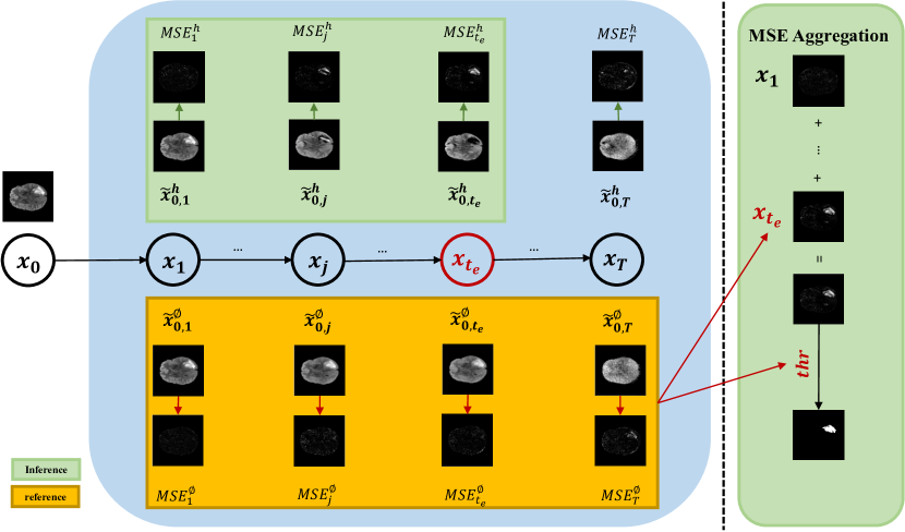
In this paper, we propose a fully weakly-supervised framework named Ano-FPDM, built upon diffusion models with classifier-free guidance [7], to eliminate the need of pixel-level labels in hyperparameter tuning. Instead of relying directly on pixel-level labels, we determine the optimal hyperparameters, such as noise scale and threshold, by leveraging the unguided forward process as a reference for the guided forward process. Our model follows the standard training process of classifier-free guidance as used in [7] with the image-level labels, i.e., healthy and unhealthy. The inference stage is illustrated in Fig. 1. Our framework utilizes the forward process of DM instead of the sampling (backward) process. During the forward process, i.e., from to , we gradually introduce noise to the input . The denoised inputs, representing the prediction of the original input from the noised input, is obtained with respect to the healthy label guidance and no guidance. The denoised inputs at step without guidance will not remove but compress the anomalous regions during forward process, i.e., a simple compression process of input . On the contrary, the denoised input with healthy label guidance removes the anomalous regions while compressing the non-anomalous regions. The two MSEs and are collected and jointly used for hyperparameter tunning. The anomaly map is derived by aggregating all for . The maximal difference between the two MSEs is used to determine the end step for the guided forward process. Here, the end step directly controls noise scale. The threshold of anomaly map is determined by the quantile of the anomaly map, which is individually selected for each input. The quantile is selected by the maximal difference between and for each input because the maximal difference is roughly linearly related to the size of the anomalous regions. A smaller quantile is selected for a larger anomalous region to include more possible pixels.
In Fig. 2, we further demonstrate our idea by an unhealthy sample from BraT21 dataset [1] and exhibit four components, i.e., , , and , in our framework. During the forward process, the anomalous regions in the path are effectively removed due to healthy label guidance. We found that the anomalous regions are more likely to be removed compared to the non-anomalous regions during forward process. In our method, we aggregate all for as our final anomaly map to increase the signal strength of anomalous regions. The rationale behind this lies in the idea that all anomaly maps in the path contribute to the same anomalous region while not all of them contribute to the same non-anomalous region. In contrast, anomalous regions persist in the path . The high frequency components are compressed before low frequency components, e.g., anomalous regions. Initially, the difference between and increases because the unguided path tends to compress high frequency details (non-anomalous region) while the healthy label guided path is more likely to remove low frequency anomalous regions. At the maximal difference, e.g., in Fig. 2, we interpret it as the low frequency anomalous regions are fully removed in the path , while all high frequency details are compressed in the path . Subsequently, the difference starts to decrease, signifying the compression of non-anomalous regions in the path and low frequency anomalous regions in the path . Consequently, we select the step that achieves the maximal difference between and as the end step . serves as a reference, indicating the completion of anomalous region removal, thereby eliminating the need for pixel-level labels.
Contributions: (i) Eliminating the need for pixel-level labels in hyperparameter tuning by using unguided denoised inputs as reference; (ii) A novel anomaly segmentation framework using the forward process of DM (iii) A novel anomaly map aggregation strategy to enhance the signal strength of anomalous regions.
Related Work Prior to the development of DM, GAN and VAE dominated the field of anomaly segmentation [16, 3, 23]. However, GAN is often criticized for their unstable training, while VAE is not ideal because of their limited expressiveness in the latent space and a tendency to produce blurry reconstructions. DM is a promising alternative due to its successes in image synthesis [4]. In the arena of unsupervised anomaly segmentation, innovations such as AnoDDPM [22] have applied the unguided denoising diffusion probabilistic model (DDPM) with simplex noise [11] to achieve notable segmentation outcomes. Furthermore, Behrendt et al. [2] have enhanced model performance by utilizing patched images as inputs to mitigate generative errors, while Iqbal et al. [8] have explored the use of masked images in both physical and frequency domains. The latent diffusion model concept, detailed by Rombach et al. [13], has been adeptly incorporated for fast segmentation in Pinaya et al. [12]. In the domain of weakly-supervised approaches, pioneering efforts by Wolleb et al. [21] have leveraged DDIM with classifier-guidance [4], a technique paralleled in Sanchez et al. [15]’s adoption of DDIM with classifier-free guidance [7], similar to the DDIB approach [19]
2 Background
2.1 Diffusion Models
During the training, the model which is parameterized by learns the unknown data distribution by adding noise to the data and subsequently denoising it. The model here is usually the U-net like architectures [14]. To be more specific, the forward process of DDPM is factorized as , which is fixed to a Markov chain with variance schedule . The transition from to is modeled as Gaussian and the distribution of transition from any arbitrary step , i.e., forward process, is in closed form
| (1) |
where , and .
The sampling process is the transition from to with the learned distribution which is the approximation of inference distribution . The forms of both distributions and are Gaussian. The training process is the minimization of KL-divergence
| (2) |
A variation of DDPM is DDIM [17]. It is non-Markovian, incorporating the input into the forward process. The inference distribution is factorized as for all . The forward process can be obtained through Bayes’ theorem in closed form:
| (3) |
where is set to 0. They both share the same objective function in training.
2.2 Classifier-free Guidance
The classifier-free guidance exhibits superior performance in generative tasks compared to classifier guidance [7]. Additionally, both training and sampling processes are simplified as it eliminates the need for an external classifier. In the sampling process, the predicted noise is replaced by the noise with guidance. For any , the predicted noise with guidance is . The parameter controls the strength of guidance. For null label , the predicted noise . The model with guidance is implemented by utilizing the extra attention mechanism [20].
3 Methodology
We utilize the forward process to extract the denoised inputs and for in terms of healthy label and null label. Then, we collect the mean square error and for further analysis. Our first step involves determining the health status of the input by assessing the cosine similarity between and . The details can be found in supplementary material. If the input is deemed unhealthy, we determine the optimal end step and threshold for segmentation.
3.1 Denoised Inputs with Classifier-free Guidance
We can add noise to the inputs in forward process with either DDPM style using Eq. 1 or DDIM style using Eq. 3 without label information. After adding the noise on step , we extract the denoised inputs with healthy guidance and without guidance by Eq. 4 and Eq. 5 respectively.
| (4) |
| (5) |
Then, we collect and .
3.2 Dynamical Noise Scale and Threshold
We use the unguided reference path to determine the appropriate end step , i.e., noise scale, for each input. It is chosen based on the maximal absolute average difference between two MSEs, i.e.,
| (6) |
Note that . To obtain the anomaly map for segmentation, we average for for all modalities, i.e., . Similarly, the segmentation threshold is individually determined for each input. We observe that the value of for is roughly linearly related to the size of tumor. Intuitively, a larger anomalous region corresponds to a larger difference value as more regions are removed. A smaller quantile is selected for a larger anomalous region to include more possible pixels. For a comprehensive understanding of our selection process, please refer to Algorithm 1, detailed in the supplementary material
4 Experiments
We train and evaluate the proposed method on BraTS21 dataset [1]. BraTS21 dataset comprises of three-dimensional Magnetic Resonance brain images depicting subjects afflicted with a cerebral tumor, accompanied by pixel-wise annotations serving as ground truth labels. Each subject undergoes scanning through four distinct MR sequences, specifically T1-weighted, T2-weighted, FLAIR, and T1-weighted with contrast enhancement. Given our emphasis on a two-dimensional methodology, our analysis is confined to axial slices. There are 1,254 patients and we split the dataset into 939 patients for training, 63 patients for validation, 252 patients for testing. We randomly select 1,000 samples in validation set for parameter tuning and 10,000 samples in testing set for evaluation. For training, we stack all four modalities while only FLAIR and T2-weighted modalities are used in inference. For preprocessing, we normalize each slice by dividing percentile foreground voxel intensity and then, pixels are scaled to the range of . Finally, all samples are interpolated to . Our model is trained as proposed in [17] with 2 Nvidia A100 80GB GPUs, and the hyperparameters are demonstrated in supplementary material. The backbone U-net is from the previous work [15].
4.1 Results: Weakly-supervised Segmentation
We report pixel-level DICE score, intersection over union (IoU) and area under the precision-recall curve (AUPRC) in terms of foreground area in Table 1. The performance on 10,000 mixed data, comprising 4,656 unhealthy samples and 5,344 healthy samples, along with the performance on all 4,656 unhealthy data are reported separately. For our method, we present results for three setups: (i) DDPM forward (stochastic encoding): Eq. 1 is used to add noise to inputs; (ii) DDIM forward (deterministic encoding): the inputs are noised by Eq. 3; (iii) tuned with labels: the hyperparameter is tuned with pixel-level labels for all inputs (non-dynamical) and noise is added using DDIM forward. For comparison methods, we report the results from AnoDDPM with Gaussian noise [22], pure DDIM, DDIM with classifier [21] and DDIM classifier-free [15]. The first two methods are only trained on healthy data and the hyperparameters of all methods are tuned by using 1000 slices in validation set. Note that our methods do not require pixel-level labels for tunning. We adopt median filter [9] and connected component filter for postprocessing. The details are provided in supplementary material. We surpass the previous methods in a quantitative evaluation. The qualitative results are shown in Fig. 4. It shows that our method can enhance the signal strength of the anomalous regions.
| Mixed | Unhealthy | |||||
| Methods | DICE | IoU | AUPRC | DICE | IoU | AUPRC |
| AnoDDPM (Gaussian)[22] | 66.1 | 61.7 | 51.8 | 37.60.1 | 28.10.1 | 61.30.1 |
| DDIM unguided | 68.40.1 | 63.7 | 54.30.1 | 40.70.7 | 31.00.1 | 63.40.1 |
| DDIM clf[21] | 76.50.1 | 71.00.1 | 58.40.3 | 52.20.2 | 40.40.2 | 61.60.2 |
| DDIM clf-free[15] | 74.3 | 69.1 | 59.9 | 49.1 | 38.1 | 61.4 |
| Ours (DDPM forward) | 77.60.1 | 71.30.1 | 72.40.1 | 56.04.0 | 45.73.5 | 76.10.1 |
| Ours (DDIM forward) | 77.8 | 72.0 | 69.7 | 54.0 | 43.5 | 72.3 |
| Ours (tuned with labels) | 77.7 | 71.8 | 69.5 | 53.2 | 42.6 | 72.4 |
4.2 Ablation Study: Hyperparameter Selection
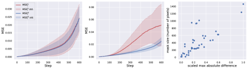
To validate the effectiveness of our chosen , we randomly select 100 unhealthy samples from the validation set and calculate the AUPRC at different steps. In Fig. 3 (a), we illustrate the change in mean and standard deviation of AUPRC over different steps. Notably, the maximal AUPRC is achieved at , supporting the feasibility of our selection. Another hyperparameter under consideration is the guidance strength . However, it does not significantly impact performance. The sensitivity of with respect to DICE is depicted in Fig. 3 (b).
5 Conclusion
In this paper, we propose a novel anomaly segmentation framework that eliminates the need for pixel-level labels in hyperparameter tuning. We utilize denoised inputs without label guidance as a reference for selecting the noise scale and dynamic threshold of the anomaly map. By aggregating anomaly maps from each forward step, we enhance the signal strength of anomaly regions, which improves the quality of anomaly maps. Our method surpasses the previous methods in terms of weakly-supervised segmentation on BraTS21 dataset.
References
- [1] Bakas, S., Reyes, M., Jakab, A., Bauer, S., Rempfler, M., Crimi, A., Shinohara, R.T., Berger, C., Ha, S.M., Rozycki, M., et al.: Identifying the best machine learning algorithms for brain tumor segmentation, progression assessment, and overall survival prediction in the brats challenge. arXiv preprint arXiv:1811.02629 (2018)
- [2] Behrendt, F., Bhattacharya, D., Krüger, J., Opfer, R., Schlaefer, A.: Patched diffusion models for unsupervised anomaly detection in brain mri. In: Medical Imaging with Deep Learning (2023)
- [3] Chen, X., You, S., Tezcan, K.C., Konukoglu, E.: Unsupervised lesion detection via image restoration with a normative prior. Medical image analysis 64, 101713 (2020)
- [4] Dhariwal, P., Nichol, A.: Diffusion models beat gans on image synthesis. Advances in neural information processing systems 34, 8780–8794 (2021)
- [5] Goodfellow, I., Pouget-Abadie, J., Mirza, M., Xu, B., Warde-Farley, D., Ozair, S., Courville, A., Bengio, Y.: Generative adversarial nets. Advances in neural information processing systems 27 (2014)
- [6] Ho, J., Jain, A., Abbeel, P.: Denoising diffusion probabilistic models. In: Proceedings of the 34th International Conference on Neural Information Processing Systems. pp. 6840–6851 (2020)
- [7] Ho, J., Salimans, T.: Classifier-free diffusion guidance. In: NeurIPS 2021 Workshop on Deep Generative Models and Downstream Applications (2021)
- [8] Iqbal, H., Khalid, U., Chen, C., Hua, J.: Unsupervised anomaly detection in medical images using masked diffusion model. In: International Workshop on Machine Learning in Medical Imaging. pp. 372–381. Springer (2023)
- [9] Kascenas, A., Pugeault, N., O’Neil, A.Q.: Denoising autoencoders for unsupervised anomaly detection in brain mri. In: International Conference on Medical Imaging with Deep Learning. pp. 653–664. PMLR (2022)
- [10] Kingma, D.P., Welling, M.: Auto-encoding variational bayes. arXiv preprint arXiv:1312.6114 (2013)
- [11] Perlin, K.: Improving noise. In: Proceedings of the 29th annual conference on Computer graphics and interactive techniques. pp. 681–682 (2002)
- [12] Pinaya, W.H., Graham, M.S., Gray, R., da Costa, P.F., Tudosiu, P.D., Wright, P., Mah, Y.H., MacKinnon, A.D., Teo, J.T., Jager, R., et al.: Fast unsupervised brain anomaly detection and segmentation with diffusion models. In: International Conference on Medical Image Computing and Computer-Assisted Intervention. pp. 705–714 (2022)
- [13] Rombach, R., Blattmann, A., Lorenz, D., Esser, P., Ommer, B.: High-resolution image synthesis with latent diffusion models. In: Proceedings of the IEEE/CVF conference on computer vision and pattern recognition. pp. 10684–10695 (2022)
- [14] Ronneberger, O., Fischer, P., Brox, T.: U-net: Convolutional networks for biomedical image segmentation. In: Medical Image Computing and Computer-Assisted Intervention (MICCAI) (2015)
- [15] Sanchez, P., Kascenas, A., Liu, X., O’Neil, A.Q., Tsaftaris, S.A.: What is healthy? generative counterfactual diffusion for lesion localization. In: MICCAI Workshop on Deep Generative Models. pp. 34–44. Springer (2022)
- [16] Schlegl, T., Seeböck, P., Waldstein, S.M., Langs, G., Schmidt-Erfurth, U.: f-anogan: Fast unsupervised anomaly detection with generative adversarial networks. Medical image analysis 54, 30–44 (2019)
- [17] Song, J., Meng, C., Ermon, S.: Denoising diffusion implicit models. In: International Conference on Learning Representations (2020)
- [18] Song, Y., Sohl-Dickstein, J., Kingma, D.P., Kumar, A., Ermon, S., Poole, B.: Score-based generative modeling through stochastic differential equations. In: International Conference on Learning Representations (2020)
- [19] Su, X., Song, J., Meng, C., Ermon, S.: Dual diffusion implicit bridges for image-to-image translation. In: The Eleventh International Conference on Learning Representations (2022)
- [20] Vaswani, A., Shazeer, N., Parmar, N., Uszkoreit, J., Jones, L., Gomez, A.N., Kaiser, Ł., Polosukhin, I.: Attention is all you need. Advances in neural information processing systems 30 (2017)
- [21] Wolleb, J., Bieder, F., Sandkühler, R., Cattin, P.C.: Diffusion models for medical anomaly detection. In: International Conference on Medical image computing and computer-assisted intervention. pp. 35–45. Springer (2022)
- [22] Wyatt, J., Leach, A., Schmon, S.M., Willcocks, C.G.: Anoddpm: Anomaly detection with denoising diffusion probabilistic models using simplex noise. In: Proceedings of the IEEE/CVF Conference on Computer Vision and Pattern Recognition. pp. 650–656 (2022)
- [23] Zimmerer, D., Isensee, F., Petersen, J., Kohl, S., Maier-Hein, K.: Unsupervised anomaly localization using variational auto-encoders. In: Medical Image Computing and Computer Assisted Interventione. pp. 289–297. Springer (2019)
Supplementary Material
A. Hyperparameter Settings
The parameters for the diffusion model used in our method are detailed in Table 2.
| Diffusion steps | 1000 |
|---|---|
| Noise schedule | linear |
| Channels | 128 |
| Heads | 2 |
| Attention resolution | 32,16,8 |
| Dropout | 0.1 |
| EMA rate | 0.9999 |
| Optimiser | AdamW |
| Learning rate | |
| , | 0.9, 0.999 |
| Batch size | 64 |
| Null label ratio | 0.1 |
| Guidance strength | 2 |
B. Byproducts of MSE Inference
Two byproducts of MSE inference are classification and threshold selection. To determine the label of inputs without the pixel-level labels, we utilize cosine similarity . Note that . In Fig. 5, we compare the MSE of healthy samples and and unhealthy samples. In the Fig. 5 (a) and (b), we observe that and in healthy samples are more similar compared to those in unhealthy samples. Consequently, we determine the threshold that achieves maximal accuracy in the validation set.
In the Fig. 5 (c), we depict the relationship between the size of the anomalous region (number of pixels) and the maximal difference value . Notably, they exhibit a relatively linear relationship. This observation serves as a rough indication of the size of the anomalous region and can be utilized for the selection of the quantile without relying on pixel-level labels. We select the segmentation quantile of the anomaly map for each input by Algorithm. 1. The input is obtained from the validation set for scaling. A smaller quantile is selected for a larger anomalous region to include more possible pixels. In our case, we select , . Then, the predicted pixel-level labels is obtained as .
C. Postprocessing
After we obtain the anomaly map, we apply a median filter with kernel size 5 to effectively enhance the performance. Then, we apply the connected component filter to remove the small connected components which is regarded as noise. We apply the same postprocessing to all methods for fair comparison.