Homogeneous turbophoresis of heavy inertial particles in turbulent flow
Abstract
Particles suspended in turbulent flows are commonly found in nature and industry, appearing as droplets, dust, or sediments. When heavier than the fluid, they possess inertia and are ejected from the most violent vortical structures of the carrier flow by centrifugal forces. Once piled up along particle paths, this small-scale mechanism leads to an effective large-scale drift. This phenomenon, known as “turbophoresis,” causes particles to leave highly turbulent regions and migrate towards calmer regions, resulting in uneven spatial distributions. This process has been extensively studied and is used to explain why particles transported by non-homogeneous flows tend to concentrate near the minima of turbulent kinetic energy.
It is demonstrated here that turbophoretic effects are just as crucial in statistically homogeneous flows. Although the average turbulent activity is uniform, instantaneous spatial fluctuations trigger local fluxes that are responsible for inertial-range inhomogeneities in the particle distribution. Direct numerical simulations are used to thoroughly probe and depict the statistics of particle accelerations, specifically their scale-averaged properties conditioned on local turbulent activity. The simulations confirm the relevance of the local energy dissipation to gauge instantaneous spatial fluctuations of turbulence. This analysis yields an effective coarse-grained dynamics, which accounts for particle detachment from the fluid and their ejection from excited regions through a space and time-dependent non-Fickian diffusion.
Such considerations lead to cast fluctuations in particle distributions in terms of a scale-dependent Péclet number , which measures the relative importance of turbulent advection compared to inertial turbophoresis at a given observation scale . Multifractal statistics of the coarse-grained turbulent energy dissipation indicate that with . Numerical simulations support this behaviour and emphasises the relevance of the turbophoretic Péclet number in characterising how particle spatial distributions, including their radial distribution function, depends on . This approach also explains the presence of voids with inertial-range sizes, and the fact that their volumes has a non-trivial distribution with a power-law tail , with an exponent that tends to 2 as . In addition to its ability to describe particle concentrations, the proposed approach provides a new framework for modelling particle transport in large-eddy simulations of turbulent flows.
keywords:
Particle/fluid flow, Isotropic turbulence, Intermittency1 Introduction
The transport of small, heavy particles by a developed turbulent flow is a common occurrence in nature and industry. Whether they are droplets in air, dust in gas, or sediments in water, these particles are often smaller than the smallest active scale of the fluid and have a larger mass density. They thus possess inertia, resulting in their detachment from the carrier fluid and uneven spatial distributions, a phenomenon known as preferential concentration. This is important in determining the interactions between these particles, such as collisions and aggregation. It also alters the transfers of momentum, kinetic energy, and heat in the particle-laden fluid. One notable example of inertial particles is water droplets in atmospheric clouds. As stressed by Jonas (1996), turbulence triggers variability in droplet sizes that can explain why the timescales for rain initiation are much shorter than those predicted by mean-field arguments. Pinsky & Khain (1997, see also ) demonstrated that the preferential concentration of droplets affects their growth by condensation and coalescence. Heterogeneities have been observed in situ (see, e.g., Kostinski & Shaw, 2001) and their small-scale effects have been quantified to improve droplet collision rates (see Reade & Collins, 2000; Falkovich et al., 2002). Still, many challenging questions raised in clouds involve interactions over a huge range of scales and thus, cannot be addressed without having recourse to large-eddy simulations (LES). Such approaches need ad-hoc parameterisations of particle dynamics and their microphysical interactions, as discussed for instance in Morrison et al. (2020). Planet formation by dust aggregation in the early Solar system is another important natural instance of inertial particles, which raises similar issues. Local fluctuations in the particle concentration trigger gravitational collapse and thus the formation of larger objects. Because of rotation around the star, dust particles migrate in large-scale anticyclonic Keplerian vortices (Gerosa et al., 2023) or in pressure bumps (Johansen et al., 2007). It is probably in these regions that primary accretions occur, but the effect of turbulence is still unclear (Johansen et al., 2015). A better understanding requires developing models to quantify dust clustering in the inertial range of turbulence (see, e.g., Hartlep & Cuzzi, 2020) and designing LES tools that cope with astrophysical specificities. Other natural situations where inertial particles occur include plankton ecology in the ocean (Seuront et al., 2001) and seed dispersion above plant canopies (Pan et al., 2014). In all cases, a precise description of large-scale fluctuations in particle density is crucial.
Equivalent questions arise in engineering. When optimising droplet vaporisation in injection sprays (Sahu et al., 2018) or monitoring particulate fouling (Henry et al., 2012), it is important to understand how inertial particles distribute over scales comparable to the larger scales of the carrier turbulent flow. The complexity of flow geometries and inhomogeneities in industrial applications give a critical role to the spatial variations of the time-averaged particle density. Much effort has thus been dedicated to derive effective transport equations for the average concentration field. In this context, Caporaloni et al. (1975) unveiled a fundamental mechanism in which turbulence inhomogeneities drive particles out of the most excited regions of the flow and concentrate them in quieter zones. They dubbed this phenomenon turbophoresis (see also Reeks, 1983), in analogy to thermophoresis, where temperature gradients cause a motion of diffusive particles toward colder regions of space. Reeks (1983, 1992) proposed closures of the kinetic equations for the particle phase-space distribution to derive effective diffusion equations for the average spatial concentration. This leads to the particle fluxes due to inertia being described by a Fick law, where the coefficient of diffusion is related to the local Lagrangian correlation of the fluid velocity. Such arguments have been successfully employed to explain why particles in turbulent channel flows tend to migrate towards the walls (see, e.g., Marchioli & Soldati, 2002; Kuerten & Vreman, 2005; Sardina et al., 2012; Fouxon et al., 2018; Brandt & Coletti, 2022). However the dependence of the diffusion coefficient on the particle Stokes number is not yet fully understood. Belan et al. (2014, see also ) showed that particles with sufficient inertia escape from low-kinetic-energy regions, leading to a localisation/delocalisation phase transition. De Lillo et al. (2016) examined the case of turbulent flows with an inhomogeneous forcing and found that turbophoretic effects are more pronounced at intermediate particle inertia. Mitra et al. (2018) interpreted this behaviour as a balance between turbophoretic and turbulent diffusions.
The applicability of turbophoresis to particle transport in flows with average inhomogeneities raises questions about its relevance in homogeneous situations. In homogeneous isotropic turbulence, instantaneous snapshots reveal spatial fluctuations of kinetic energy throughout the inertial range. Meanwhile, particle distributions display heterogeneous concentrations characterised by large-scale quasi-uniform regions, localised voids, and sheet-like clusters, as observed for instance by Eaton & Fessler (1994). To quantify inertial-range particle distributions, different observables are needed compared to those used for the dissipative range. At small scales, particle distributions exhibit multifractal scaling properties (see Hogan et al., 1999; Bec et al., 2011; Schmidt et al., 2017; Bec et al., 2024) and are fully characterised by a dimension spectrum that depends solely on the Stokes number. The unified picture of the joint dependence on length scale and response time arises from the fact that dissipative-range dynamics involve a unique timescale determined by the typical amplitude of velocity gradients. This is in contrast with the hierarchy of timescales involved in inertial-range physics. In the two-dimensional inverse cascade, Boffetta et al. (2004) found that particles concentrate quasi uniformly on thin filamentary structures separated by voids whose distribution follows a universal scaling law. However, in the random, white-in-time, self-similar flows considered by Bec et al. (2007b), such scaling is absent, and particle distributions are characterised by local fractal dimensions determined by the scale-dependent Stokes number (Balkovsky et al., 2001), defined by non-dimensionalising the particle response time by the turnover time at the observation scale . Both of these scenarios coexist in three-dimensional turbulence, as pointed up by Bec et al. (2007a), Yoshimoto & Goto (2007), or inferred from the sweep-stick mechanism of Goto & Vassilicos (2008). The intricate spatial correlations of the pressure gradient, or equivalently of the fluid acceleration, play a key role. By using Voronoï tesselations, Monchaux et al. (2010, 2012) introduced a definition of particle clusters and found that their size distribution follows a universal scaling law independent of the Stokes number. This was confirmed by Baker et al. (2017), who showed that clusters preferentially sample regions of the flow with higher strain and lower vorticity. However, Bragg et al. (2015) found that this statistical bias depends on inertia and is actually quantified by the scale-dependent Stokes number . These arguments led them to predict scale invariance for two-particle statistics when , which was confirmed by Hartlep et al. (2017) using a cascade multiplier approach. Ariki et al. (2018) further argued that the pair correlation function follows a universal power-law using a Lagrangian renormalisation closure. The wavelet analysis conducted by Matsuda et al. (2021) shows intermittent particle densities, with a stronger contribution from voids observed at smaller spatial scales. However, the question of whether scale invariance holds in the inertial-range distributions of particles and, if so, which mechanisms are involved, remains ambiguous.
To shed new lights on these issues, an appropriate effective model for inertial-range particle dynamics is expected to be useful. While there are various simplified approaches to dilute particle suspensions, reviewed for instance by Balachandar & Eaton (2010), the Eulerian field representations of the particle phase proposed by Ferry & Balachandar (2001) provide promising tools. In this approach, the particle velocity is enslaved to the carrier phase, with the effect of inertia being regarded as a compressible correction proportional to the fluid velocity acceleration. While this approximation has often shown its relevance, it remains limited to the asymptotics of small particle inertia, and it combines very different timescales, as acceleration is influenced by dissipative-range physics. Fevrier et al. (2005) extended these considerations to large Stokes numbers by assuming that the particle motion can be seen as the sum of a mesoscopic velocity and a random component. The latter term corresponds to a diffusive motion, is uncorrelated in space, and has been found to properly reproduce particle properties when their response time is much larger than the turbulent large-eddy turnover time. This contribution, dubbed random uncorrelated motion by Reeks et al. (2006), was used by Gustavsson et al. (2012) in synthetic random flows and shown to suitably describe the effect of fold caustics on the particle kinetics. This approach relies on the idea that turbulence has only a cumulative effect along particle paths, as long as the latter have a sufficiently long correlation time. However, fluctuations do not need to be averaged over times prescribed by the particles lag, but this procedure can rather stem from a spatial or temporal coarse-graining of the turbulent field, thus incorporating the effect of instantaneous spatial inhomogeneities.
We aim here to present a model that can effectively describe and quantify particle dynamics in the inertial range of a fully developed turbulent flow. Small-scale detachments from the fluid result in particles carrying forward past fluctuations instead of filtering them out in a time-reversible manner. Building on the phenomenology introduced by Bec & Chétrite (2007), we argue that this mechanism cumulates over time, leading to an ejection process that causes non-Fickian particle fluxes. Our proposed model utilizes an Itô, rather than Stratonovich, diffusion process with a diffusion coefficient that varies based on the local flow activity. This statistically homogeneous turbophoresis can be used to quantify inhomogeneities in the particle distribution and, to some extent, reconcile the various viewpoints discussed above. Our analysis is grounded in the results of direct numerical simulations conducted at large Reynolds numbers and relies on a comprehensive evaluation of particle accelerations.
The paper is structured as follows. In §2 we introduce our settings and discuss the relevant observables for our analysis. We also provide a general appreciation of the correlations between particle concentrations and instantaneous inhomogeneities in turbulent activity. In §3 we develop a Lagrangian perspective and conduct a detailed statistical analysis of particle acceleration. In §4 we shift our focus to the Eulerian frame and derive an effective equation for the particle coarse-grained density. From this model, we draw properties of the inertial-range distribution and discuss specifically the implications of this approach to the distribution of voids. Finally, in §5 we summarise our findings and discuss possible perspectives.
2 Models, simulations, and spatial coarse-graining
2.1 Homogeneous isotropic turbulence and energy dissipation
We investigate the behaviour of particles passively suspended in a three-dimensional fluid flow. The velocity field of the fluid, denoted by , satisfies the incompressible Navier–Stokes equations
| (1) |
where represents the pressure, is the mass density of the fluid, is its kinematic viscosity, and is an external volume force. The force is prescribed with homogeneous and isotropic statistics and is correlated on large scales in both space and time. The force injects kinetic energy into the flow at an average rate of . We perform direct numerical simulations of (1) using the pseudo-spectral code LaTu on the triply periodic box and employ third-order Runge–Kutta time marching. The details of the code can be found in Homann et al. (2007). Two sets of simulations are carried out with different resolutions. Corresponding numerical and turbulent parameters are presented in table 1.
After a certain period of time, the fluid velocity field reaches a statistical steady state characterised by multifractal statistics of the local dissipation rate (see, e.g., Frisch, 1995). This is evidenced from the scale-dependent statistics of the coarse-grained dissipation obtained by averaging the local dissipation over the ball of center and diameter , that is . For , the probability distribution of takes the form
| (2) |
where is the multifractal spectrum, which can be interpreted as the dimension of the fractal set on which the scale-averaged dissipation is when , and corresponds to the weight associated with each singularity exponent . In Kolmogorov 1941 phenomenology, there are no fluctuations of and except for , for which .
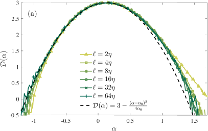
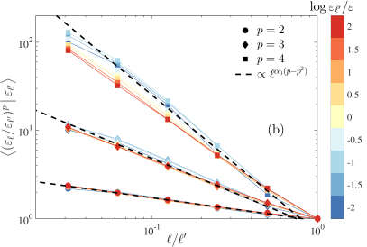
Figure 1(a) shows the multifractal spectrum obtained from numerical measurements of . We find that lognormal statistics, for which the dimension spectrum is a parabola , provide a good approximation for the lowest values of . It is however known that lognormal distributions have several shortcomings due to the non-conservative nature of the cascade models on which they are based (see discussion in Frisch, 1995, §8.6.5). Despite this, such an approximation is still useful for estimating moderate-order statistics, well beyond the central-limit approximation. Using Kolmogorov (1962) refined similarity hypothesis, and recent confirmations by Lawson et al. (2019), the statistics of the fluid velocity relate to the fluctuations of . For the longitudinal structure functions , the lognormal approximation with parameter predicts a scaling behaviour with . For obtained from our simulations, we get , , , which are in good agreement with experimentally measured values (see Saw et al., 2018, for a recent review).
Multifractal statistics are often interpreted phenomenologically as resulting from the random multiplicative cascade experienced by the coarse-grained dissipation. This scenario suggests that the probability distribution (2) should also apply to the fluctuations of conditioned on the observed value of at the same location but over a larger scale . As shown in figure 1(b) for , numerical simulations confirm this feature, revealing a scaling regime with an exponent that is closely approximated by the lognormal prediction. These multiscale statistics play a crucial role in investigating the coarse-grained dynamics of transported particles, as we will discuss in more detail later on.
2.2 Particles, preferential sampling and concentrations
After the fluid flow reaches a statistical steady state, we introduce heavy, inertial, point-like particles that are homogeneously seeded with velocities equal to that of the fluid at their positions. The trajectories of these particles follow
| (3) |
Particles are assumed much smaller than the Kolmogorov dissipative scale , and sufficiently massive to neglect so added-mass, Magnus, and history effects. The viscous drag intensity is given by the response time , where is the particle mass density and its diameter. This time is used to define the Stokes number , with denoting Kolmogorov dissipative timescale. The Stokes number measures particle inertia. When , the particles almost follow the flow and behave as tracers. When , they detach from the flow and behave ballistically. We adopt a Lagrangian approach in our simulations, where particles trajectories are tracked by integrating Eq. (3) with the fluid velocity at their location obtained by linear interpolation from the grid. We use 10 different values of the Stokes number in the range and, for each value of St, a number of particles that roughly corresponds to one particle per box of size .
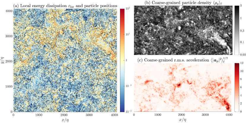
Upon reaching a statistically stationary state, the particle distributions exhibit highly non-uniform patterns and strongly correlate with the turbulent structures of the flow, as depicted in figure 2(a). The spatial arrangement of particles shows voids in the most active regions of the flow, where dissipation is high, sheet-like clusters that encapsulate these voids, and quasi-uniform distributions in regions with lower turbulent intensity. These concentration fluctuations are attributed to the inertial-range motions of particles, as the sizes of the regions are much larger than the dissipative scale . To filter out dissipative-range effects, we introduce the coarse-grained particle density . It is obtained by counting the number of particles in small boxes of size , which define a partition of the spatial domain. Figure 2(b) shows obtained with . The spatial variations of particle dynamics also serve as a marker for the different regions of the flow. In figure 2(c), we show the coarse-grained root-mean-square acceleration obtained by averaging the squared modulus of acceleration for all particles located in given boxes of size . Particle voids correspond clearly to high accelerations, indicating that concentration fluctuations are caused by detachment from the fluid and expulsion from active regions. It is worth noting that this mechanism is distinct from the conventional picture of inertial ejection from simple vortices by centrifugal forces, as the thickness of vortex filaments is several times smaller than the coarse-graining scale .
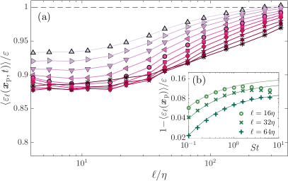
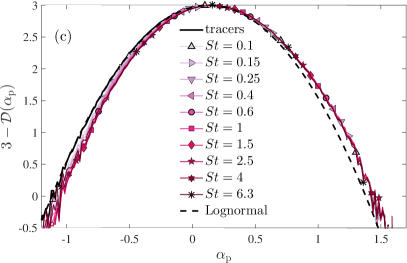
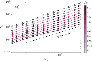
Particle concentration in regions of low turbulent activity can be further quantified by measuring the preferential sampling of energy dissipation by the particles. The mean value of computed along the paths of particles with different Stokes numbers is shown as a function of the coarse-graining scale in figure 3(a). Particles sample preferentially regions where is lower than the average dissipation , even when their inertia is weak – see figure 3(b). This bias persists in the inertial range, indicating that it stems from agitation accumulated along particle paths rather than instantaneous ejection from the flow small-scale structures. Measurements of the multifractal spectrum evaluated at particle positions confirm this tendency, as shown in figure 3(c) for . The dependence on St is weak and visible only at negative values of the singularity exponent corresponding to the most violent events. At positive values of , the dimension spectra associated with different Stokes numbers are almost undistinguishable. This suggests that preferential sampling results from the expulsion of particles from the most singular regions rather than convergence toward calmer ones.
The observed correlations between the dynamical and concentration properties of particles and the instantaneous inertial-range inhomogeneities of the turbulent flow suggest that the underlying mechanisms are akin to turbophoresis in non-homogeneous flows, at least qualitatively. Specifically, particles tend to move away from regions with high turbulent activity, forming voids, and follow the fluid in calmer zones. To provide quantitative support for these ideas, we aim to develop effective equations for an averaged particle density. In the study of turbophoresis in non-homogeneous flows, these equations are obtained by averaging over either the realisations of turbulence or time in statistically stationary and ergodic situations. However, such classical averages are not applicable to instantaneous particle distribution in homogeneous turbulence. Nevertheless, we expect that a similar effective dynamics can be derived from a low-pass-filtered viewpoint, where the coarse-grained average plays a central role.
3 Non-homogeneous diffusion of Lagrangian trajectories
We revisit here the classical approach used to develop stochastic Langevin models for turbulent transport (see, e.g., Minier, 2016, for a review). The approach is based on the assumption that while Lagrangian velocities are correlated over timescales of the order of the integral timescale, acceleration become uncorrelated much faster, justifying an approximation of trajectories as diffusive processes. We begin in §3.1 by providing effective approximations for the second-order statistics of fluid acceleration. We then extend these approximation to inertial particles in §3.2, specifically to describe their spatially-averaged acceleration. Finally, in §3.3, we argue that the coarse-grained dynamics of particles can be approximated as a diffusion process with a space-dependent diffusion coefficient.
3.1 Fluid acceleration
Turbulent accelerations of fluid particles are one of the most striking signatures of intermittency. At the turn of the century, significant advances in direct numerical simulations and in particle-tracking experimental techniques have enabled to investigate acceleration statistics in detail (see Toschi & Bodenschatz, 2009, for a review). These studies revealed that the variance of acceleration deviates from its dimensional estimate and exhibits a notable dependence on Reynolds number. Specifically, it can be expressed as , where accounts for this dependence. Hill (2002b) found that at moderate values of the Reynolds number, Taylor’s scaling gives , assuming that acceleration is dominated by pressure gradients. At large , intermittency prevails and , where can be estimated using multifractal approaches (see, e.g., Borgas, 1993; Sawford et al., 2003; Biferale et al., 2004). The log-normal approximation of §2.1 yields for . To match these two asymptotics, we introduce the ad hoc approximation:
| (4) |
Figure 4(a) compares this fit to numerical measurements by Gotoh & Fukayama (2001), Bec et al. (2006), and Yeung et al. (2006), together with current simulations. The approximation (4) with , , and provides a reasonably good agreement.

We now examine the spatial correlations of acceleration, which will be important in approximating particle displacement later. In an isotropic flow, the correlation tensor components in the longitudinal and transverse directions to a given separation are interrelated. In a homogeneous and isotropic flow, depends only on the distance and satisfies (Obukhov & Yaglom, 1951; Hill & Wilczak, 1995)
| (5) |
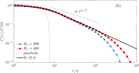
where summation is assumed over repeated indices. This relation assumes that pressure gradients dominate acceleration and uses Poisson equation to express them in terms of velocity gradients. In homogeneous isotropic flow, the right-hand side of (5) can be expressed as , where is the fourth-order structure function. Since , we expect acceleration correlations to decrease as when . Therefore, we get , which is steeper than the K41 prediction proposed by Obukhov & Yaglom (1951). Figure 4(b) shows the spatial correlations of acceleration for our two numerical simulations. Our data are consistent with the experimental measurements of Xu et al. (2007) and display a power-law with an even steeper exponent close to .
This behaviour extends beyond the transition scale introduced by Hill (2002a), which is derived from the Taylor expansion of correlations at small separations. Equation (5) yields
| (6) |
Hence, the correlation function can be approximated to leading order as as approaches zero. Here, with is the length scale characterising the parabolic decay of the acceleration correlations, analogous to the Taylor microscale for velocity correlations. It is worth noting that both and exhibit an intermittent dependence on the Reynolds number. While scales as at large Reynolds numbers, scales as (with , see Nelkin, 1990). Consequently, we have . Using the multifractal lognormal approximation, we obtain and , which yields , consistent with the prediction of Hill (2002a). Our numerical simulations reveal that for and for , confirming a weak dependence on Reynolds number. Nevertheless, as shown in figure 4(b), deviations from the predicted inertial-range scaling persist for scales much larger than .
We interpret the observed behaviour as an extended contribution from small scales to the integral relation (6). For , the first term always gives a contribution , obtained by evaluating the integral over the interval . Furthermore, separations in the inertial range contribute to both integrals a term , with a universal constant determined by the 4th-order structure function, independent of Reynolds number. Balancing these two terms, we find that the first contribution is dominant as long as , which is satisfied for where . The lognormal approximation gives , which is smaller than , consistently ensuring that . This second crossover scale is much larger than , hence ensuring the existence of a range of separations over which the correlations of acceleration behave as and this range increases with . The numerical data of figure 4(b) confirm this picture. The scaling observed at extends further in the inertial range as increases, and corresponds to with a constant that depends weakly on . Both this regime and the small-scale parabolic approximation of the correlation can be matched by the following ad hoc formula
| (7) |
This approximation, shown as a solid line in figure 4(b), is in good agreement with numerical data. In the following, we will use this formula to coarse-grain the particle dynamics.
3.2 Particle accelerations
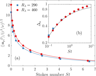
We focus here on the statistical properties of the acceleration of inertial particles. Figure 5(a) shows its variance as a function of the Stokes number. Our measurements agree with those of Bec et al. (2006) and, as they span larger values of the Reynolds numbers, they allow us to substantiate and extend several observations made in that work.
First, we observe that our data, corresponding to two different Reynolds numbers, collapse reasonably well on the top of each other when plotted as a function of St and rescaled by the acceleration variance of tracers. This can be seen in figure 5(b), which shows the relative discrepancy in acceleration variance . Although a weak Reynolds-number dependence is noticeable at very small Stokes numbers, one difficulty distinguishes deviations from possible statistical or numerical errors. Therefore, most effects of intermittency are accounted for by the factor introduced in §3.1. This suggests that acceleration variance can be approximated as , where is a non-dimensional function of the Stokes number with no significant dependence on .
The second observation is an abrupt reduction in the acceleration variance at small but finite values of St. There is a drop of over 25% from to , which we interpret as a consequence of preferential sampling, specifically of particle ejection from violent small-scale vortical structures. Our data suggest that the relative discrepancy increases faster than any a power law of St. This is evidenced by its convexity when plotted in log-log in figure 5(b), indicating that the acceleration variance may have an essential singularity at . Such a dependence on Stokes number has been observed previously for the rate at which fold caustics occur (Wilkinson et al., 2006), a phenomenon also coined sling effect (Falkovich et al., 2002). These same events drive the abrupt depletion observed for energy dissipation in §2.2 and here for acceleration variance. Figures 3(b) and 5(b) show that both discrepancies are well-fitted by a curve , where depends weakly on . This can be interpreted as a contribution from the probability that the local Stokes number is sufficiently large for the particle to detach from the flow, and thus that . At high , the distribution of turbulent velocity gradients is known to display stretched-exponential tails with an exponent (see Yeung et al., 2018), consistent with the behaviour of . However, Buaria et al. (2019) found that the constant in the exponential has a significant dependence on the Reynolds number. Therefore, to further refine our discussion, it will be necessary to better understand this dependence in future studies.
Deviation to this singular behaviour occurs at . Preferential sampling becomes less important, and acceleration statistics are dominated by the particle delay on the flow: their velocity is given by low-pass filtering the fluid velocity over timescales smaller than (see Bec et al., 2006). Gorokhovski & Zamansky (2018) used such considerations to estimate , where the last relation assumes and uses the inertial-range scaling of the second-order Lagrangian structure function. Consequently, the variance of acceleration approaches a power-law when .
The two asymptotics and can be matched by the ad hoc formula
| (8) |
which, as seen from figure 5(a), gives a fairly good approximation of particle acceleration variance up to . Note that this fitting formula differs from other proposals, such as the one suggested by Gorokhovski & Zamansky (2018), which aimed to also capture response times larger than the large-eddy turnover time . As the response times of our particles lie below (i.e. are such that ), we use hereafter equation (8).
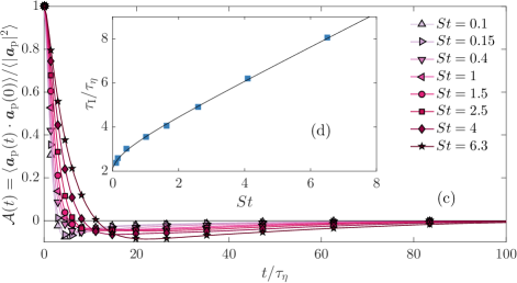
We now turn to two-time statistics of the particle acceleration, focusing on the autocorrelation . The results are shown in figure 5(c). Figure 5(d) shows the integral time as a function of St. At small Stokes numbers, it approaches the value for tracers, . Deviations occur due again to preferential sampling. Ejection from small-scale vortical structures leads to particles concentrating in regions where the local dissipative timescale is larger than its average. Dimensionally, we expect and, assuming that , we get for . On the other hand, for large Stokes numbers, the particle response time effectively filters out all the flow timescales below it, resulting in . These two regimes can be matched using the fitting formula
| (9) |
where is the value measured from tracers, is obtained from the acceleration variance, and provides a good agreement with the data of figure 5(d).
To complete this survey, we finally examine the spatially averaged particle acceleration . This quantity is defined as the mean acceleration over all particles that are at time within a ball of diameter centred at position . We are particularly interested in the statistics of conditioned on the spatially averaged dissipation rate obtained in the same ball at the same time. This allows us to investigate the relationship between the local fluctuations of small-scale quantities, such as acceleration, and the inertial-range fluctuations of the dissipation field, in accordance with Kolmogorov’s refined similarity hypothesis. According to dimensional analysis, the conditional statistics of the coarse-grained acceleration , once normalised by , depend only on the local Stokes number and the local Reynolds number .
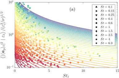

We can express the conditional mean-squared coarse-grained acceleration of particles as
Based on our earlier analysis of the spatial correlations of the fluid acceleration and the approximation (7), we can assume that for , where is the cut-off scale of acceleration spatial correlations associated with the local conditioning dissipation . The conditional acceleration variance is obtained from (8) by replacing , and St with their local values , and given by the spatially-averaged dissipation. Using with , we obtain
| (10) |
with . This approximation is valid for , , and . Local fluctuations about this average are described by the coarse-grained variance of acceleration, which we can obtain by replacing the dissipation rate with the conditioning value in (8). We get
| (11) |
Figure 6 shows scatter plots of the conditional mean-squared coarse-grained acceleration and the coarse-grained variance of acceleration obtained from numerical simulations. The solid lines in the figure represent the predictions (10) and (11), which are based on the approximations made in the preceding text and fitted parameters. The close agreement between the numerical data and the predictions supports the validity of our approximations.
3.3 An effective diffusion process
To derive effective equations for the particle coarse-grained dynamics, we combine all ingredients from previous analyses. Using equation (3), we can write the particle velocity as , allowing us to express its displacement over a time as
| (12) |
We choose to be much smaller than the Lagrangian correlation time of to ensure that the fluid velocity along particle path does not vary significantly in . Thus, the first integral in the right-hand side of (12) can be approximated as . All fluctuations and dependences on particle inertia are entailed in the second integral. Additionally, if we assume that is much longer than the correlation time of the particle acceleration, we can apply the central-limit theorem and write
where is the outer product and denotes a multivariate normal random variable with mean and covariance matrix . The Lagrangian time average introduced here is obtained by time integration along particle paths over the interval , assuming the limit . It contains information about the turbulent state in which the particle is at the initial time and is crucial to account for inertial-range fluctuations. To estimate this time average, we use an Eulerian spatial average over a coarse-graining scale , so that . This estimate assumes that is chosen of the order of the turnover time associated with , and hence that . Preferential sampling by particles, which naturally arises from the Lagrangian average, is now accounted for by evaluating the Eulerian average at the current particle position .
Under these assumptions, we can now express the particle displacement as
| (13) |
Here, denotes the increment of the three-dimensional Wiener process, and is a tensorial diffusion coefficient that satisfies
| (14) |
This diffusion coefficient not only depends on the particle response time and the coarse-graining scale, but also fluctuates in space and time. Taking the limit while keeping , we can write the effective displacement (13) as the stochastic differential equation:
| (15) |
where is given by (14). The diffusion appears here as a multiplicative noise, which we define using the Itô convention. This is imposed by the requirement that in the statistical steady state, the average particle velocity should vanishes, i.e. . Since and , the contribution of noise should vanish as well.
The proposed model (15) for particle dynamics share some similarities with the model introduced by Fevrier et al. (2005). In both cases, the drift term, the “mesoscopic Eulerian particle velocity” in their work, is the sum of the fluid velocity and a residual one. In our model, this residual velocity is proportional to the filtered particle acceleration. Both models also include a noise term. However, while the “quasi-Brownian velocity” of Fevrier et al. (2005) satisfies a molecular chaos assumption and is uncorrelated in space, we identify it in our model as a diffusion with a space-time dependent coefficient that fluctuates due to turbulent agitation. As a result, this contribution is correlated over inertial-range separations.
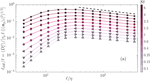
Particle inertia affect both drift and diffusion in the stochastic equation (15). These two contributions have different weights at different scales. They balance each other at a scale , estimated as . Diffusion dominates at scales smaller than and is negligible at larger scales. Thus, the diffusion term is relevant only when is larger than the coarse-graining scale . Using considerations on acceleration from the previous subsection, we can approximate for
| (16) |
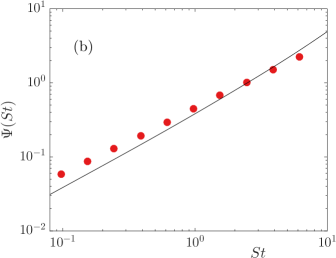
The exponent is negative, indicating that the diffusive scale becomes very small when the coarse-graining scale is far inside the inertial range. Numerical measurements of , reported in figure 7(a), obtained from the coarse-grained statistics of particle acceleration, confirm the power-law behaviour (16) at . We also observe that, for the moderate values of the Stokes number considered, is always smaller than . Based on previous acceleration correlation measurements, we expect that the constant behaves as
| (17) |
This prediction, shown as solid curve in figure 7(b), compares well with the numerical measurements shown as circles. Extrapolating this behaviour to higher Stokes numbers, we obtain that , implying that neglecting diffusion requires choosing a coarse-graining scale such that . Note that this condition applies to particle response times in the inertial range but still smaller than the fluid velocity Lagrangian correlation time . This condition is more restrictive than the classical idea that the particle response time should be smaller than the eddy turnover time associated with the coarse-graining scale, which would instead lead to .
In this section, we have shown that the coarse-grained dynamics of inertial particles can be approximated using an effective stochastic equation that includes both drift and diffusion terms. The terms that arise due to particle inertia and account for the differences between the particle and fluid dynamics are governed by the coarse-grained particle acceleration, which fluctuates in both space and time and serves as a clear indicator of turbulent activity. We have also established that for sufficiently large spatial-averaging scale, or equivalently small Stokes numbers, diffusive effects become negligible. In the following section, we will focus on this asymptotics and develop a further level of modelling that will allow us to derive an effective dynamics for the Eulerian coarse-grained density of particles.
4 Particle transport as an Eulerian ejection process
4.1 Model dynamics for the particle density
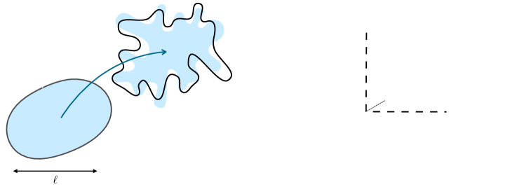
In the previous section, we introduced an effective velocity field , which describes the Lagrangian dynamics of particles for a large enough coarse-graining scale (corresponding to the limit of weak inertia). This approach can be reformulated in a Eulerian frame by considering the evolution of the coarse-grained particle density in a volume of size — figure 8(a). We adopt a quasi-Lagrangian approach and follow the control volume in its motion with the fluid velocity , while considering its exchanges with its Eulerian neighbours. To evaluate the fluxes due to particles inertia at the boundary of the control volume, we distinguish between outgoing and incoming fluxes. Some particles leave the volume because they have acquired a large-enough acceleration inside , and the outgoing flux should thus be controlled by the coarse-grained acceleration computed inside the reference volume. This flux can be expressed as
| (18) |
Here, denotes the Heaviside function, is the unit vector normal to the surface of , and the average is taken over accelerations satisfying to account only for outgoing particles. Assuming isotropic distribution of the outgoing flux, this signed average can be approximated by . The control volume is chosen as a cube with edge length , and the spatial domain is tiled by such cubes — figure 8(b). The time evolution of the mass of particles contained in the cell is then given by
| (19) | |||||
denotes here the material derivative along the trajectories of fluid elements. Mass is lost from the outgoing flux in the reference cell and gained from the outgoing flux coming from its six neighbours on the cubic tiling. The right-hand side of equation (19) corresponds to the discrete Laplacian of the outgoing flux . By considering the mass evolution on scales much larger than the coarse-graining scale , we can write a continuous limit which reads
| (20) |
The position- and time-dependent coarse-grained diffusion coefficient, , appears inside the Laplacian as expected for an ejection process. This model for particle transport provides a quantitative extension of the phenomenological ideas proposed in Bec & Chétrite (2007). As we will discuss later, the underlying ejection process gives rise to specific features in the probability distribution of the spatially-averaged density, .
The diffusive term in equation (20) can be expressed as the divergence of the flux vector , which consists of two distinct contributions. The first corresponds to osmotic forces, resulting in classical Fickian diffusion that enhances mixing alongside fluid advection. The second arises from turbophoretic forces due to convection by the velocity , which drive particles from regions with high , characterised by strong particle accelerations and high turbulent activity, to regions with low . The turbophoretic contribution is responsible for the preferential sampling of particles in the inertial-range, as qualitatively discussed in §2.2. To determine whether turbophoretic forces are strong enough to induce significant concentration fluctuations and inertial-range voids, we need to compare the magnitudes of the terms in . In particular, turbophoretic forces dominate when , which implies that the scale of variation of the diffusion coefficient (and thus of the particle acceleration) should be smaller than that of density.

The balance between fluid flow convection and turbophoretic diffusion can be characterised at a given coarse-graining scale by a dimensionless Péclet number that we define as
| (21) |
Here, is the typical fluid velocity fluctuation at scale , which is estimated by the square-root of the second-order longitudinal structure function . In the inertial-range, with . Equation (10) shows that for the spatially-averaged acceleration, , which leads to the scaling behaviour with for coarse-graining scales in the inertial range. Figure 9(a) confirms this power-law dependence. Regarding the dependence on the Stokes number, we have when , as shown in figure 9(b). The numerical data indicate that the Péclet number can reach values larger than 1 for both and . The scaling laws for small Stokes number and large averaging scale give , which results in a Péclet number much higher than unity when . This scaling is distinct from those discussed in the previous section based on Lagrangian considerations.
4.2 Distribution of the coarse-grained density
Based on our previous arguments, we anticipate that for sufficiently large scales, the Péclet number defined in (21) captures alone dependences upon both the Stokes number St and the coarse-graining scale . This asymptotic regime corresponds to the range of parameter values where the approximation (20) accurately describes particle dynamics, and we expect that their clustering behaviour will primarily depend on .
We start with examining the radial distribution function, or pair distribution function , which describes the probability of finding two particles at a distance , normalised by the probability for a uniform distribution. It can be expressed through the second-order moment of the coarse-grained density , namely . For a uniform distribution, we have , so . Deviations from uniformity as a function of the scale-dependent Péclet number are shown in figure 10(a). Data associated with different values of the Stokes number collapse onto a unique master curve, when the coarse-graining scale is chosen far enough in the inertial range. This curve shows two distinct scaling regimes: one at moderate Péclet numbers and another at large values.
For large values of , we can express the coarse-grained density as with . To leading order, the perturbation satisfies . For statistically stationary deviations to uniformity, we get , which implies that and the variance scales as . At lower Péclet numbers and higher Stokes numbers, when deviations to uniformity are still small, the velocity contribution is dominated by the large-scale advection, so we have . This means that deviations from uniformity depend on , but not on fluid velocity fluctuations at the scale . Thus, we have . Using , we obtain the second scaling regime . A solid curve in figure 10(a) shows an ad-hoc approximation matching these two asymptotic laws. It provides a reasonable fit to the numerical measurements.

Let us contextualise our results with respect to previous findings on how particles recover a uniform distribution at large scales. When becomes large, tends to unity and in our approach, we find that . Such an algebraic dependence differs from the exponential decay proposed by Reade & Collins (2000) that seems confirmed by the experimental measurements of Petersen et al. (2019, see also ). The scaling that we observe also significantly deviates from the prediction of Balkovsky et al. (2001, see also ), who proposed that the radial distribution depends primarily on the scale-dependent Stokes number, with when . However, the relevance of has so far been demonstrated only in models assuming the fluid velocity is a white noise process. For instance, for velocities in the Kraichnan ensemble, it has been shown by Bec et al. (2007b) that , which is not a pure function of . Moreover, the direct numerical simulations of Bec et al. (2007a) at moderate Reynolds numbers suggest that particle distributions primarily depend on a scale-dependent contraction rate , without clear evidence of scaling for the radial distribution function in the inertial range. More recent numerics by Bragg et al. (2015) and Ariki et al. (2018) indicate a scaling , albeit with uncertainties on the Stokes number dependence. Our approach reveals a second power-law regime, persisting up to , where , potentially masquerading a behaviour . It would be of interest to reassess previous measurements of the radial distribution function in the light of present findings.
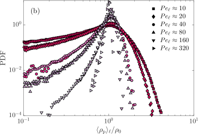
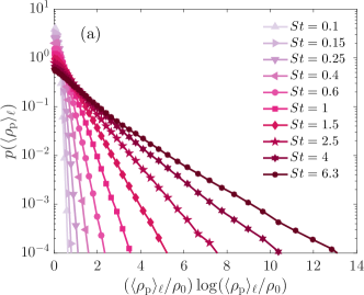
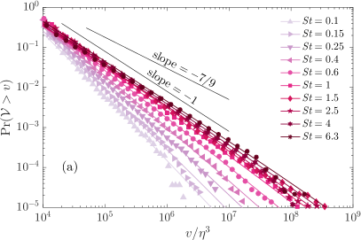
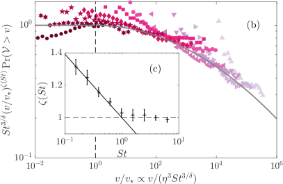
To complement our analysis, we turn to the probability density function of the coarse-grained density. Figure 10(b) displays numerical measurements for six different high values of the Péclet number. Remarkably, data obtained from various combinations of the particle response time and the coarse-graining scale , resulting in the same , exhibit a reasonable collapse, within the range of statistical errors. This confirms the significance of the scale-dependent Péclet number in characterising density fluctuations. The observed probability distributions manifest distinctive features. Both tails, associated with small and large values of , are broader than those expected for a Poisson distribution corresponding to a uniform particle density. These deviations can be explained by the ejection process framework developed in Bec & Chétrite (2007). Specifically, we find that large densities occur more frequently than the quasi-Gaussian tail of the Poisson distribution. The probability density functions exhibit a sub-exponential behaviour , which is clearly captured by our data, as evident in figure 11(a).
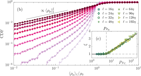
Regarding the left tail, quasi-empty regions occur also more frequently than in a simple Poisson process. Density distributions follow there a power-law , as depicted in figure 11(b). This behaviour is again a characteristic feature of ejection processes. To provide a heuristic explanation, we consider the approximation (20) of the dynamics, where the evolution of the coarse-grained density along a particle trajectory is given by
We can thus write the cumulative distribution of the Lagrangian density for as
Here, we have decomposed the Lagrangian integral of the turbophoretic term into a sum of equally-distributed independent random variables , where represents the correlation time of the ejection rate along particle paths. The asymptotic behaviour is then obtained by optimising , which represents the number of times mass must be ejected to create a void. If this number is of the order of unity, the above formula samples the (negative) tail of the distribution of . A power-law behaviour arises because it is more favourable to choose a value of of the order of , indicating that empty regions are more likely to results from persistent ejections rather than rare, violent events leading to instantaneous voids. Thus, by writing the optimum as with , the cumulative distribution function becomes
When the Péclet number is large enough, advection dominates, resulting in the correlation time being given by the eddy-turnover time at scale . Consequently, for . Furthermore, the exponent is bounded from below by in order for the probability distribution of to be normalisable. Eulerian statistics are then obtained by accounting for the additional factor of involved in the Lagrangian average, because it is itself weighted by the particle density. This finally leads to write the probability distribution of the Eulerian coarse-grained density as
| (22) |
where is a positive constant. Figure 11(c) displays the measured exponent as a function of the scale-dependent Péclet number. The exponent saturates at for and becomes positive above that threshold, increasing as with for larger values, confirming the prediction given by equation (22).
4.3 Distribution of voids
We now shift out attention to the large voids that prominently emerge in the spatial distribution of particles. As we observed in §2.2, the sizes of these empty regions span the entire inertial range, even at moderate Stokes numbers. Our goal here is to investigate to what extent the statistics of these voids can be explained by the effective diffusion (20) introduced in §4.1.
To detect these voids numerically, we rely on the spatially-averaged density. They are defined as connected sets of empty cells, identified by a label-propagation algorithm. The volume of each void is determined by counting the number of cubes with a volume that it encompasses. While alternative techniques for void detection, such as Delaunay tessellations (see, e.g., Gaite, 2005), may offer better algorithmic efficiency and the ability to define voids in a parameter-free manner, they yield the same results as presented below. Therefore, we have chosen to continue working with the spatially-averaged density, which is central to the model for particle coarse-grained dynamics proposed in §4.1. Figure 12 displays two-dimensional slices of the three-dimensional distribution of voids for a coarse-graining scale of and for three different values of the particle response time. These distributions are shown at the same instant of time and in the same slice as the local kinetic energy dissipation rate in figure 2(a). The comparison of these two figures clearly identifies voids as regions with high turbulent activity. Furthermore, there are evident correlations between the empty regions associated with different Stokes numbers. One such correlation can be observed for the circled greenish structure, where the intensity of voids increases with St. Conversely, in other cases, exemplified by the lower orangish structure circled with dots, a void that exists at small St can be filled by particles with a larger inertia.
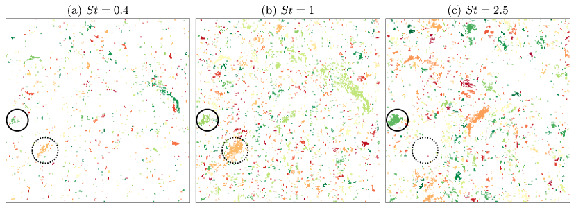
Figure 13(a) presents the complementary cumulative probability distributions of void volumes obtained for different Stokes numbers and an elementary coarse-graining scale . These distributions exhibit broad tails at large inertial-range volumes, displaying a distinctive power-law behaviour , where is particularly evident for the highest Stokes number values. These statistics remain robust when using alternative definitions of voids, or when changing either the total number of particles or the coarse-graining scale . Similar power-law dependencies have been previously observed in the probability distribution of void sizes. In the two-dimensional inverse cascade, Boffetta et al. (2004) found an intermediate regime where the probability density function of void areas behaves as , independent of the Stokes number, with an exponential cutoff at larger sizes. Goto & Vassilicos (2006) proposed a self-similar distribution of void areas with , arising from sweep-stick mechanisms where particles preferentially trace fluid zero-acceleration points. Extending these arguments to three dimensions, Yoshimoto & Goto (2007) predicted a power-law exponent for the cumulative distribution of void volumes, with reasonable numerical support at moderate values of the Reynolds number. Figure 13(a) showcases this behaviour for comparison. Additional evidence supporting this shallow trend comes from grid-turbulence experiments by Sumbekova et al. (2017) and analyses employing Voronoï diagrams, where they found for void areas in two-dimensional cross-sections of the three-dimensional particle distribution. Assuming a relationship of the form with , these observations suggest . However, our data clearly show a steeper slope, even for Stokes numbers exceeding those considered in both Yoshimoto & Goto (2007) and Sumbekova et al. (2017).
We revisit here void statistics in light of the ejection process that we introduced to model particle dynamics in the inertial range. The probability that the volume of a void exceeds the value can be estimated as the probability of finding very few particles in a cube of size . This implies that the coarse-grained density is there of the order of or smaller than . Thus, we can write . Using the asymptotic behaviour (22) for the distribution of at small values, we obtain
Choosing to be of the order of , we have , resulting in
| (23) |
Here, is a positive constant, , and the exponent has a logarithmic dependence on the Stokes number of the form , where . Figure 13(a) shows such predictions for the distribution of void volumes along with numerical data. Reasonable agreement is obtained by choosing for fitting parameters , , , and . The measurements shown in the right-hand panel of figure 13 corroborate these values. Figure 13(b) represents the rescaled complementary cumulative distribution of void volumes as a function of . Despite statistical noise, data associated with various Stokes numbers (symbols) seem to collapse for onto the log-normal master curve (solid line). The measured exponent is represented in figure 13(c). It follows for and saturates to for larger St.
It is worth noting that the intermediate power-law behaviour that we observe in the distribution of void sizes can be interpreted in terms of Zipf’s law (see, e.g., Cristelli et al., 2012). Samples following this law exhibit coherence and adhere to certain dynamical constraints, which are satisfied when the size dynamics of the objects under consideration can be described as a multiplicative process. In the context of turbophoresis, interpreted as an ejection process, this framework naturally emerges, as the mass of particles ejected from a given cell is proportional to its volume. For such a coherent process, the exponent represents a classical case. It arises when large voids are formed through the merging of smaller, independent voids with uncorrelated histories, as may occur at large Stokes numbers. The growth rate of a large void becomes proportional to the probability of intersecting other empty regions, which, in turn, is proportional to its volume. This process, known as “preferential attachment”, leads to an exponent of (see De Marzo et al., 2021).
5 Concluding remarks
In this paper, we have presented convincing evidence that the phenomenon of turbophoresis, previously thought to occur only in turbulent flows containing inhomogeneities, also manifests in statistically homogeneous situations. This effect arises from the instantaneous non-uniformities intrinsic to turbulent flows, spanning the whole inertial range. Our direct numerical simulations clearly illustrate the ejection of inertial particles from highly active regions of the flow, leading to their concentration in calmer regions. Remarkably, this behaviour persists in spatially coarse-grained representations of both the flow and the particles, resulting in strong correlations between the spatially-averaged particle concentration and the fluctuations in turbulent kinetic energy dissipation within the inertial range.
The fluctuations in particle acceleration play a crucial role in the turbophoresis process. When particles experience pure Stokes drag, these acceleration fluctuations govern their deviations from fluid motion. Through analytical and phenomenological arguments, as well as a detailed analysis of numerical simulations, we have gained insights into the statistics of particle acceleration. This includes understanding spatial and temporal correlations, as well as the influence of fluid flow intermittency on second-order statistics. Building upon these insights, we have introduced approximations for the inertial-range dynamics of particles in terms of effective diffusion equations with a diffusivity that varies in both space and time. The diffusion coefficient is expressed in terms of the coarse-grained particle acceleration, which, in turn, is determined by local turbulent activity. These approximations hold when spatial averaging scales are sufficiently large or particle inertia is sufficiently small, ensuring that higher-order corrections to this dynamics remain negligible. In this asymptotic regime, the dynamics of particles depend solely on a local Péclet number that quantifies the relative importance of advection by the fluid flow compared to inertia-induced diffusion at a given coarse-graining scale . Notably this Péclet number exhibits a non-trivial power-law dependence on the observation scale, , where the exponent is prescribed by the intermittent statistics of the fluid velocity and deviates significantly from the value that would be obtained by dimensional analysis.
The diffusive models we have developed provide means to infer of the distribution of particles in the inertial range. Specifically, we demonstrate that the statistics of the coarse-grained particle density at a given inertial-range scale depend solely on the scale-dependent Péclet number . Furthermore, these diffusive models predict that the probability density functions of exhibit algebraic tails at small values and allow for the characterisation of the associated exponent as a function of . For large masses, the models predict a super-exponential behaviour that is also well reproduced by our direct numerical simulations. However, statistics that span different scales, such as the distribution of voids, display more intricate dependencies. Nonetheless, we find that the probability distribution of void volumes follows a power law with exponent steeper than at intermediate values, transitioning to a log-normal tail at larger values. Our direct numerical simulations demonstrate a reasonably good agreement with this prediction, emphasising the need to revisit previous work on void statistics in the light of these potential behaviours.
The introduction of space-dependent diffusions in this study presents a novel framework for incorporating inertial particles into models or large-eddy simulations of turbulent flows. The coarse-grained particle density can be effectively approximated using diffusion equations derived from spatial averaging, with a fluctuating diffusion coefficient determined by the local turbulent dissipation rate. To test, calibrate, and validate this approach, further numerical simulations that integrate the effective advection-diffusion equations at various coarse-graining resolutions are necessary. Although beyond the scope of this work, this perspective holds promise for future work.
[Funding]Computational resources were provided by GENCI (grant IDRIS 2019-A0062A10800) and by the OPAL infrastructure from Université Côte d’Azur. This work received support from the UCA-JEDI Future Investments, funded by the French government (grant no. ANR-15-IDEX-01), and from the Agence Nationale de la Recherche (grant no. ANR-21-CE30-0040-01).
References
- Ariki et al. (2018) Ariki, T., Yoshida, K., Matsuda, K. & Yoshimatsu, K. 2018 Scale-similar clustering of heavy particles in the inertial range of turbulence. Phys. Rev. E 97, 033109.
- Baker et al. (2017) Baker, L., Frankel, A., Mani, A. & Coletti, F. 2017 Coherent clusters of inertial particles in homogeneous turbulence. J. Fluid Mech. 833, 364–398.
- Balachandar & Eaton (2010) Balachandar, S. & Eaton, J.K. 2010 Turbulent dispersed multiphase flow. Annu. Rev. Fluid Mech. 42, 111–133.
- Balkovsky et al. (2001) Balkovsky, E., Falkovich, G. & Fouxon, A. 2001 Intermittent distribution of inertial particles in turbulent flows. Phys. Rev. Lett. 86, 2790–2793.
- Bec et al. (2006) Bec, J., Biferale, L., Boffetta, G., Celani, A., Cencini, M., Lanotte, A., Musacchio, S. & Toschi, F. 2006 Acceleration statistics of heavy particles in turbulence. J. Fluid Mech. 550, 349–358.
- Bec et al. (2007a) Bec, J., Biferale, L., Cencini, M., Lanotte, A., Musacchio, S. & Toschi, F. 2007a Heavy particle concentration in turbulence at dissipative and inertial scales. Phys. Rev. Lett. 98, 084502.
- Bec et al. (2011) Bec, J., Biferale, L., Cencini, M., Lanotte, A.S. & Toschi, F. 2011 Spatial and velocity statistics of inertial particles in turbulent flows. In J. Phys: Conf. Ser., , vol. 333, p. 012003.
- Bec et al. (2007b) Bec, J., Cencini, M. & Hillerbrand, R. 2007b Clustering of heavy particles in random self-similar flow. Phys. Rev. E 75, 025301.
- Bec & Chétrite (2007) Bec, J. & Chétrite, R. 2007 Toward a phenomenological approach to the clustering of heavy particles in turbulent flows. New J. Phys. 9, 77.
- Bec et al. (2024) Bec, J., Gustavsson, K. & Mehlig, B. 2024 Statistical models for the dynamics of heavy particles in turbulence. Annu. Rev. Fluid Mech. 56, 189–213.
- Belan (2016) Belan, S. 2016 Concentration of diffusional particles in viscous boundary sublayer of turbulent flow. Physica A 443, 128–136.
- Belan et al. (2014) Belan, S., Fouxon, I. & Falkovich, G. 2014 Localization-delocalization transitions in turbophoresis of inertial particles. Phys. Rev. Lett. 112, 234502.
- Biferale et al. (2004) Biferale, L., Boffetta, G., Celani, A., Devenish, B.J., Lanotte, A. & Toschi, F. 2004 Multifractal statistics of Lagrangian velocity and acceleration in turbulence. Phys. Rev. Lett 93, 064502.
- Boffetta et al. (2004) Boffetta, G., De Lillo, F. & Gamba, A. 2004 Large scale inhomogeneity of inertial particles in turbulent flows. Phys. Fluids 16, L20–L23.
- Borgas (1993) Borgas, M.S. 1993 The multifractal Lagrangian nature of turbulence. Phil. Trans. Roy. Soc. London A 342, 379–411.
- Bragg et al. (2015) Bragg, A.D., Ireland, P.J. & Collins, L.R. 2015 Mechanisms for the clustering of inertial particles in the inertial range of isotropic turbulence. Phys. Rev. E 92 (2), 023029.
- Brandt & Coletti (2022) Brandt, L. & Coletti, F. 2022 Particle-laden turbulence: progress and perspectives. Annu. Rev. Fluid Mech. 54, 159–189.
- Buaria et al. (2019) Buaria, D., Pumir, A., Bodenschatz, E. & Yeung, P.-K. 2019 Extreme velocity gradients in turbulent flows. New J. Phys. 21, 043004.
- Caporaloni et al. (1975) Caporaloni, M., Tampieri, F., Trombetti, F. & Vittori, O. 1975 Transfer of particles in nonisotropic air turbulence. J. Atmos. Sci. 32, 565–568.
- Cristelli et al. (2012) Cristelli, M., Batty, M. & Pietronero, L. 2012 There is more than a power law in Zipf. Sci. Rep. 2, 1–7.
- De Lillo et al. (2016) De Lillo, F., Cencini, M., Musacchio, S. & Boffetta, G. 2016 Clustering and turbophoresis in a shear flow without walls. Phys. Fluids 28, 035104.
- De Marzo et al. (2021) De Marzo, G., Gabrielli, A., Zaccaria, A. & Pietronero, L. 2021 Dynamical approach to Zipf’s law. Phys. Rev. Res. 3, 013084.
- Eaton & Fessler (1994) Eaton, J.K. & Fessler, J.R. 1994 Preferential concentration of particles by turbulence. Int. J. Multiphase Flow 20, 169–209.
- Falkovich et al. (2002) Falkovich, G., Fouxon, A. & M., Stepanov 2002 Acceleration of rain initiation by cloud turbulence. Nature 419, 151–154.
- Falkovich et al. (2003) Falkovich, G., Fouxon, A. & Stepanov, M. 2003 Statistics of turbulence-induced fluctuations of particle concentration. In Sedimentation and Sediment Transport (ed. A. Gyr & W. Kinzelbach), pp. 155–158. Dordrecht: Springer.
- Ferry & Balachandar (2001) Ferry, J. & Balachandar, S. 2001 A fast Eulerian method for disperse two-phase flow. Int. J. Multiphase Flow 27, 1199–1226.
- Fevrier et al. (2005) Fevrier, P., Simonin, O. & Squires, K.D. 2005 Partitioning of particle velocities in gas-solid turbulent flows into a continuous field and a spatially uncorrelated random distribution: theoretical formalism and numerical study. J. Fluid Mech. 533, 1–46.
- Fouxon et al. (2018) Fouxon, I., Schmidt, L., Ditlevsen, P., van Reeuwijk, M. & Holzner, M. 2018 Inhomogeneous growth of fluctuations of concentration of inertial particles in channel turbulence. Phys. Rev. Fluids 3, 064301.
- Frisch (1995) Frisch, U. 1995 Turbulence: the legacy of A.N. Kolmogorov. Cambridge, UK: Cambridge University Press.
- Gaite (2005) Gaite, J. 2005 Zipf’s law for fractal voids and a new void-finder. Eur. Phys. J. B 47, 93–98.
- Gerosa et al. (2023) Gerosa, F.A., Méheut, H. & Bec, J. 2023 Clusters of heavy particles in two-dimensional Keplerian turbulence. Eur. Phys. J. Plus 138 (1), 9.
- Gorokhovski & Zamansky (2018) Gorokhovski, M. & Zamansky, R. 2018 Modeling the effects of small turbulent scales on the drag force for particles below and above the kolmogorov scale. Phys. Rev. Fluids 3, 034602.
- Goto & Vassilicos (2006) Goto, S. & Vassilicos, J.C. 2006 Self-similar clustering of inertial particles and zero-acceleration points in fully developed two-dimensional turbulence. Phys. Fluids 18, 115103.
- Goto & Vassilicos (2008) Goto, S. & Vassilicos, J.C. 2008 Sweep-stick mechanism of heavy particle clustering in fluid turbulence. Phys. Rev. Lett. 100, 054503.
- Gotoh & Fukayama (2001) Gotoh, T. & Fukayama, D. 2001 Pressure spectrum in homogeneous turbulence. Phys. Rev. Lett. 86, 3775.
- Gustavsson et al. (2012) Gustavsson, K., Meneguz, E., Reeks, M.W. & Mehlig, B 2012 Inertial-particle dynamics in turbulent flows: caustics, concentration fluctuations and random uncorrelated motion. New J. Phys. 14, 115017.
- Hartlep & Cuzzi (2020) Hartlep, T. & Cuzzi, J.N. 2020 Cascade model for planetesimal formation by turbulent clustering. Astrophy. J. 892, 120.
- Hartlep et al. (2017) Hartlep, T., Cuzzi, J.N. & Weston, B. 2017 Scale dependence of multiplier distributions for particle concentration, enstrophy, and dissipation in the inertial range of homogeneous turbulence. Phys. Rev. E 95, 033115.
- Henry et al. (2012) Henry, C., Minier, J.-P. & Lefèvre, G. 2012 Towards a description of particulate fouling: From single particle deposition to clogging. Adv. Colloid Interface Sci. 185, 34–76.
- Hill (2002a) Hill, R.J. 2002a Length scales of acceleration for locally isotropic turbulence. Phys. Rev. Lett. 89 (17), 174501.
- Hill (2002b) Hill, R.J. 2002b Scaling of acceleration in locally isotropic turbulence. J. Fluid Mech. 452, 361–370.
- Hill & Wilczak (1995) Hill, R.J. & Wilczak, J.M. 1995 Pressure structure functions and spectra for locally isotropic turbulence. J. Fluid Mech. 296, 247–269.
- Hogan et al. (1999) Hogan, R.C., Cuzzi, J.N. & Dobrovolskis, A.R. 1999 Scaling properties of particle density fields formed in simulated turbulent flows. Phys. Rev. E 60, 1674.
- Homann et al. (2007) Homann, H., Dreher, J. & Grauer, R. 2007 Impact of the floating-point precision and interpolation scheme on the results of DNS of turbulence by pseudo-spectral codes. Comput. Phys. Comm. 177, 560–565.
- Johansen et al. (2015) Johansen, A., Jacquet, E., Cuzzi, J.N., Morbidelli, A. & Gounelle, M. 2015 New paradigms for asteroid formation. In Asteroids IV (ed. P. Michel et al.), pp. 471–492. Univ. of Arizona, Tucson.
- Johansen et al. (2007) Johansen, A., Oishi, J.S., Mac Low, M.-M., Klahr, H., Henning, T. & Youdin, A. 2007 Rapid planetesimal formation in turbulent circumstellar disks. Nature 448, 1022–1025.
- Jonas (1996) Jonas, P.R. 1996 Turbulence and cloud microphysics. Atmos. Res. 40, 283–306.
- Kolmogorov (1962) Kolmogorov, A.N. 1962 A refinement of previous hypotheses concerning the local structure of turbulence in a viscous incompressible fluid at high Reynolds number. J. Fluid Mech. 13, 82–85.
- Kostinski & Shaw (2001) Kostinski, A.B. & Shaw, R.A. 2001 Scale-dependent droplet clustering in turbulent clouds. J. Fluid Mech. 434, 389–398.
- Kuerten & Vreman (2005) Kuerten, J.G.M. & Vreman, A.W. 2005 Can turbophoresis be predicted by large-eddy simulation? Phys. Fluids 17, 011701.
- Lawson et al. (2019) Lawson, J.M., Bodenschatz, E., Knutsen, A.N., Dawson, J.R. & Worth, N.A. 2019 Direct assessment of Kolmogorov’s first refined similarity hypothesis. Phys. Rev. Fluids 4, 022601.
- Marchioli & Soldati (2002) Marchioli, C. & Soldati, A. 2002 Mechanisms for particle transfer and segregation in a turbulent boundary layer. J. Fluid Mech. 468, 283–315.
- Matsuda et al. (2021) Matsuda, K., Schneider, K. & Yoshimatsu, K. 2021 Scale-dependent statistics of inertial particle distribution in high reynolds number turbulence. Phys. Rev. Fluids 6, 064304.
- Minier (2016) Minier, J.-P. 2016 Statistical descriptions of polydisperse turbulent two-phase flows. Phys. Rep. 665, 1–122.
- Mitra et al. (2018) Mitra, D., Haugen, N.E.L. & Rogachevskii, I. 2018 Turbophoresis in forced inhomogeneous turbulence. Eur. Phys. J. Plus 133, 1–8.
- Monchaux et al. (2010) Monchaux, R., Bourgoin, M. & Cartellier, A. 2010 Preferential concentration of heavy particles: a Voronoï analysis. Phys. Fluids 22 (10), 103304.
- Monchaux et al. (2012) Monchaux, R., Bourgoin, M. & Cartellier, A. 2012 Analyzing preferential concentration and clustering of inertial particles in turbulence. Int. J. Multiphase Flow 40, 1–18.
- Morrison et al. (2020) Morrison, H., van Lier-Walqui, M., Fridlind, A.M., Grabowski, W.W., Harrington, J.Y., Hoose, C., Korolev, A., Kumjian, M.R., Milbrandt, J.A., Pawlowska, H. & others 2020 Confronting the challenge of modeling cloud and precipitation microphysics. J. Adv. Model. Earth Syst. 12, e2019MS001689.
- Nelkin (1990) Nelkin, M. 1990 Multifractal scaling of velocity derivatives in turbulence. Phys. Rev. A 42, 7226–7229.
- Obukhov & Yaglom (1951) Obukhov, A.M. & Yaglom, A.M. 1951 The microstructure of turbulent flow. Prikl. Mat. Mekh. 15, 3–26.
- Pan et al. (2014) Pan, Y., Chamecki, M. & Isard, S.A. 2014 Large-eddy simulation of turbulence and particle dispersion inside the canopy roughness sublayer. J. Fluid Mech. 753, 499––534.
- Petersen et al. (2019) Petersen, A., Baker, L. & Coletti, F. 2019 Experimental study of inertial particles clustering and settling in homogeneous turbulence. J. Fluid Mech. 864, 925––970.
- Pinsky & Khain (1997) Pinsky, M.B. & Khain, A.P. 1997 Turbulence effects on droplet growth and size distribution in clouds—a review. J. Aerosol Sci. 28, 1177–1214.
- Reade & Collins (2000) Reade, W.C. & Collins, L.R. 2000 A numerical study of the particle size distribution of an aerosol undergoing turbulent coagulation. J. Fluid Mech. 415, 45–64.
- Reeks (1983) Reeks, M.W. 1983 The transport of discrete particles in inhomogeneous turbulence. J. Aerosol Sci. 14, 729–739.
- Reeks (1992) Reeks, M.W. 1992 On the continuum equations for dispersed particles in nonuniform flows. Phys. Fluids A 4, 1290–1303.
- Reeks et al. (2006) Reeks, M.W., Fabbro, L. & Soldati, A. 2006 In search of random uncorrelated particle motion (rum) in a simple random flow field. In Proc. 2006 ASME Joint US European Fluids Engineering Summer Meeting, pp. 1755–1762. Fluids Engineering Division Summer Meeting.
- Sahu et al. (2018) Sahu, S., Hardalupas, Y. & Taylor, A.M.K.P. 2018 Interaction of droplet dispersion and evaporation in a polydispersed spray. J. Fluid Mech. 846, 37–81.
- Sardina et al. (2012) Sardina, G., Schlatter, P., Brandt, L., Picano, F. & Casciola, C.M. 2012 Wall accumulation and spatial localization in particle-laden wall flows. J. Fluid Mech. 699, 50–78.
- Saw et al. (2018) Saw, E.-W., Debue, P., Kuzzay, D., Daviaud, F. & Dubrulle, B. 2018 On the universality of anomalous scaling exponents of structure functions in turbulent flows. J. Fluid Mech. 837, 657–669.
- Sawford et al. (2003) Sawford, B.L., Yeung, P.K., Borgas, M.S., Vedula, P., La Porta, A., Crawford, A.M. & Bodenschatz, E. 2003 Conditional and unconditional acceleration statistics in turbulence. Phys. Fluids 15, 3478–3489.
- Schmidt et al. (2017) Schmidt, L., Fouxon, I. & Holzner, M. 2017 Inertial particles distribute in turbulence as Poissonian points with random intensity inducing clustering and supervoiding. Phys. Rev. Fluids 2, 074302.
- Seuront et al. (2001) Seuront, L., Schmitt, F. & Lagadeuc, Y. 2001 Turbulence intermittency, small-scale phytoplankton patchiness and encounter rates in plankton: where do we go from here? Deep Sea Res. 48, 1199–1215.
- Shaw (2003) Shaw, R.A. 2003 Particle-turbulence interactions in atmospheric clouds. Annu. Rev. Fluid Mech. 35, 183–227.
- Sumbekova et al. (2017) Sumbekova, S., Cartellier, A., Aliseda, A. & Bourgoin, M. 2017 Preferential concentration of inertial sub-Kolmogorov particles: the roles of mass loading of particles, Stokes numbers, and Reynolds numbers. Phys. Rev. Fluids 2, 024302.
- Toschi & Bodenschatz (2009) Toschi, F. & Bodenschatz, E. 2009 Lagrangian properties of particles in turbulence. Annu. Rev. Fluid Mech. 41, 375–404.
- Wilkinson et al. (2006) Wilkinson, M., Mehlig, B. & Bezuglyy, V. 2006 Caustic activation of rain showers. Phys. Rev. Lett. 97 (4), 048501.
- Xu et al. (2007) Xu, H., Ouellette, N.T., Vincenzi, D. & Bodenschatz, E. 2007 Acceleration correlations and pressure structure functions in high-Reynolds number turbulence. Phys. Rev. Lett. 99, 204501.
- Yeung et al. (2006) Yeung, P.-K., Pope, S.B., Lamorgese, A.G. & Donzis, D.A. 2006 Acceleration and dissipation statistics of numerically simulated isotropic turbulence. Phys. Fluids 18, 065103.
- Yeung et al. (2018) Yeung, P.-K., Sreenivasan, K.R. & Pope, S.B. 2018 Effects of finite spatial and temporal resolution in direct numerical simulations of incompressible isotropic turbulence. Phys. Rev. Fluids 3, 064603.
- Yoshimoto & Goto (2007) Yoshimoto, H. & Goto, S. 2007 Self-similar clustering of inertial particles in homogeneous turbulence. J. Fluid Mech. 577, 275.