Spectroscopy by Tensor Renormalization Group Method

Abstract

We present a spectroscopy scheme for the lattice field theory by using tensor renormalization group method combining with the transfer matrix formalism. By using the scheme, we can not only compute the energy spectrum for the lattice theory but also determine quantum numbers of the energy eigenstates. Furthermore, wave function of the corresponding eigenstate can also be computed. The first step of the scheme is to coarse-grain the tensor network of a given lattice model by using the higher order tensor renormalization group, and then after making a matrix corresponding to a transfer matrix from the coarse-grained tensors, its eigenvalues are evaluated to extract the energy spectrum. Secondly, the quantum number of the eigenstates can be identified by a selection rule that requires to compute matrix elements of an associated insertion operator. The matrix elements can be represented by an impurity tensor network and computed by the coarse-graining scheme. Moreover, we can compute the wave function of the energy eigenstate by putting the impurity tensor at each point in space direction of the network. Additionally, the momentum of the eigenstate can also be identified by computing an appropriate matrix elements represented by tensor network. As a demonstration of the new scheme, we show the spectroscopy of $(1+1)$d Ising model and compare it with exact results. We also present a scattering phase shift obtained from two-particle state energy using Lüscher’s formula.

1 Introduction

Computing the energy spectrum and eigenstates is a fundamental and important task when studying a given quantum system. For example, in lattice QCD (Quantum chromodynamics), where the Monte Carlo method is usually used, the hadron spectrum is obtained by computing the two-point function of a given insertion operator that belongs to a desired quantum channel. The methodology of the hadron spectroscopy has been well developed so far [1, 2] and the numerical results are in good agreement with the experimental values [3], but there are unavoidable practical difficulties in the method. For instance, when one wants to accurately obtain the lowest energy gap, the Euclidean time extent should be taken quite large to suppress the effect of higher excited states. Furthermore, if one wants to extract the energy spectrum of higher excited states, very large statistics are required to suppress the statistical noise. Motivated by these difficulties, we look for alternative numerical tools for the spectroscopy. A potential candidate is tensor network method (see [4, 5, 6] for review) that can be classified into two groups: Hamiltonian formalism [7, 8, 9, 10, 11, 12, 13] and Lagrangian formalism [14, 15, 16, 17, 18, 19, 20, 21, 22, 23, 24, 25, 26, 27, 28, 29, 30, 31, 32, 33, 34, 35, 36, 37, 38, 39, 40, 41, 42, 43, 44]. For example, the spectroscopy using the former was done in [45, 46] for $(1+1)$d QED (Quantum electrodynamics). On the other hand, the spectroscopy for the latter is discussed in [47, 48], but the quantum number identification was not addressed. In the current work we will complete the spectroscopy using the Lagrangian formalism and this is the main purpose of the paper.

Our new spectroscopy scheme starts by considering the transfer matrix formalism. In principle, a direct diagonalization of the transfer matrix provides us the exact energy spectrum of a system and it does not require the large time extent in contrast to the Monte Carlo method. The transfer matrix itself, however, has a very large dimensionality and it increases exponentially with respect to the volume of a system. In order to reduce the dimensionality, we employ the Tensor Renormalization Group (TRG) method that uses the information compression technique based on the singular value decomposition. So far many TRG coarse-graining algorithms are proposed [49, 50, 51, 52, 53, 54, 55, 56, 57, 58, 59, 60, 61, 62, 63], but we here choose the Higher Order Tensor Renormalization Group (HOTRG) [50] since it has relatively high accuracy and can be extended into higher dimensional systems. By using the new scheme, we are not only able to compute the energy spectrum but also classify the quantum number of the energy eigenstates. The latter procedure can be done by a selection rule that is derived from a symmetry of the system. A crucial quantity in the selection rule is the matrix element of an interpolating operator associated with the symmetry. The matrix element can be represented by the tensor network with some impurity and evaluated by the coarse-graining scheme. Moreover, we can compute the wave function of the energy eigenstate from the matrix element where a proper operator is inserted at each point in the space direction of the lattice. From the position dependence of the wave function, we can infer the momentum of the state. We will demonstrate the new scheme by applying to $(1+1)$d Ising model and show that the energy spectrum and the quantum number are correctly reproduced by comparing with the exact results [64]. Furthermore, we will show a scattering phase shift obtained from the two-particle state energy using Lüscher’s formula [65, 66, 67, 68, 69, 70, 71, 72, 73].

The rest of the paper is organized as follows. Theoretical basics are summarized in Sec. 2. We briefly remind the spectroscopy using the correlation function in Sec. 2.1 and the transfer matrix formalism in Sec. 2.2. In Sec. 2.3, we explain how to numerically obtain the energy spectrum and how to identify the quantum number of energy eigenstate by using tensor renormalization group method and this is a key section of the paper. The numerical results for $(1+1)$d Ising model are given in Sec. 3 where the energy spectrum, the quantum number classification, momentum identification, and the scattering phase shift are presented in Sec. 3.1, 3.2, 3.3, and 3.4 respectively. Summary is given in the final section. In Appendix A, we summarize the transfer matrix and the tensor network representation for the Ising model. The exact spectrum of the transfer matrix for the Ising model is summarized in Appendix B.

2 Formulation

2.1 Spectroscopy using correlation function

Let us briefly remind how to obtain the energy spectrum from a correlation function [1, 2]. In the continuum Euclidean space-time with time extent $T$, the correlation function for an interpolating operator is defined as

$$\langle\hat{\cal O}^{\dagger}_{q}(\tau)\hat{\cal O}_{q}(0)\rangle=\frac{{\rm Tr}\left[\hat{\cal O}^{\dagger}_{q}(\tau)\hat{\cal O}_{q}(0)e^{-\hat{H}T}\right]}{{\rm Tr}[e^{-\hat{H}T}]}$$ (1)

where $\hat{\cal O}_{q}(\tau)$ is the Euclidean time Heisenberg operator whose quantum number is denoted by $q$,

$$\hat{\cal O}_{q}(\tau)=e^{\hat{H}\tau}\hat{\cal O}_{q}(0)e^{-\hat{H}\tau}$$ (2)

and $\hat{H}$ is the Hamiltonian of a system. In a finite spatial volume, the eigenvalue of $\hat{H}$ is discretized

$$\hat{H}|n,q^{\prime}\rangle=E_{n,q^{\prime}}|n,q^{\prime}\rangle$$ (3)

for $n=0,1,2,\cdots$ and for all possible quantum numbers $q^{\prime}$. The spectral decomposition of the numerator in the correlation function is given by

$${\rm Tr}\left[\hat{\cal O}^{\dagger}_{q}(\tau)\hat{\cal O}_{q}(0)e^{-\hat{H}T}\right]=\sum_{m,n=0}^{\infty}\sum_{q^{\prime},q^{\prime\prime}}|\langle n,q^{\prime\prime}|\hat{\cal O}_{q}(0)|m,q^{\prime}\rangle|^{2}e^{-(T-\tau)E_{m,q^{\prime}}}e^{-\tau E_{n,q^{\prime\prime}}}.$$ (4)

For large $T$ limit, in the summation of $m$ and $q^{\prime}$, the ground state, that is, the minimum energy eigenstate of the vacuum channel $(m,q^{\prime})=(0,{\rm vac})$ dominates the summations

$${\rm Tr}\left[\hat{\cal O}^{\dagger}_{q}(\tau)\hat{\cal O}_{q}(0)e^{-\hat{H}T}\right]\stackrel{{\scriptstyle T\to\infty}}{{\sim}}\sum_{n=0}^{\infty}\sum_{q^{\prime\prime}}|\langle n,q^{\prime\prime}|\hat{\cal O}_{q}(0)|\Omega\rangle|^{2}e^{-(T-\tau)E_{\Omega}}e^{-\tau E_{n,q^{\prime\prime}}}$$ (5)

where the ground state is denoted by $|\Omega\rangle=|0,{\rm vac}\rangle$. Furthermore, thanks to the conservation of quantum numbers, $q^{\prime\prime}=q$ sector only survives

$$\langle n,q^{\prime\prime}|\hat{\cal O}_{q}(0)|\Omega\rangle\neq 0\hskip 14.22636pt\mbox{ for }q^{\prime\prime}=q$$ (6)

and other matrix elements vanish, thus we have

$${\rm Tr}\left[\hat{\cal O}^{\dagger}_{q}(\tau)\hat{\cal O}_{q}(0)e^{-\hat{H}T}\right]\stackrel{{\scriptstyle T\to\infty}}{{\sim}}\sum_{n=0}^{\infty}|\langle n,q|\hat{\cal O}_{q}(0)|\Omega\rangle|^{2}e^{-(T-\tau)E_{\Omega}}e^{-\tau E_{n,q}}.$$ (7)

In total, by taking into account the denominator, the correlation function in the $T\to\infty$ limit is given by

$$\lim_{T\to\infty}\frac{{\rm Tr}\left[\hat{\cal O}^{\dagger}_{q}(\tau)\hat{\cal O}_{q}(0)e^{-\hat{H}T}\right]}{{\rm Tr}[e^{-\hat{H}T}]}=\sum_{n=0}^{\infty}|\langle n,q|\hat{\cal O}_{q}(0)|\Omega\rangle|^{2}e^{-\tau(E_{n,q}-E_{\Omega})}.$$ (8)

In a usual Monte Carlo (MC) simulation for the hadron spectroscopy, one computes the correlation function with a proper interpolating operator for several time separations then the energy gaps,

$$\omega_{n,q}=E_{n,q}-E_{\Omega}$$ (9)

are extracted from the data. Such a computation requires the large time extent as well as the large time separation to avoid the contamination due to the higher excited states. Furthermore, it is usually difficult to extract the energy of the higher excited states, thus one needs sophisticated methods, say, the variational method [65] and so on.

2.2 Transfer matrix formalism for lattice field theory

Needless to say, the computation of the correlation function is not the only way to obtain the energy spectrum. A more direct method is the diagonalization of the Hamiltonian or equivalently the transfer matrix. In fact, this method does not require computing the correlation function or increasing the time extent in contrast to the MC calculation. In this subsection, we briefly remind the transfer matrix formalism for lattice field theory. In the following, the lattice spacing is set to $a=1$.

For simplicity here we consider the field theory on the two-dimensional lattice, although the discussion here can be straightforwardly extended to higher dimensional systems. As a concrete example we consider the lattice scalar field theory with the nearest-neighbor interaction and similar argument can be straightforwardly applied to fermion or gauge systems. The scalar fields $\phi({\bm{r}})$ reside on the square lattice ${\bm{r}}=(t,x)\in\Gamma$ where the lattice $\Gamma$ is defined

$$\Gamma=\{(t,x)|t=0,1,2,\cdots,L_{\tau}-1\,\,{\rm and}\,\,x=0,1,2,\cdots,L_{x}-1\}$$ (10)

and the periodic boundary condition (PBC) is imposed on all directions. Here $0$-direction ($1$-direction) is considered as time (space) direction. The partition function of the system is given by

$$Z=\int\prod_{{\bm{r}}\in\Gamma}d\phi({\bm{r}})e^{-S[\phi]}$$ (11)

where the lattice action is given by

$$S[\phi]=\sum_{{\bm{r}}\in\Gamma}\left[\sum_{\mu=0}^{1}\frac{1}{2}\left(\phi({\bm{r}}+\hat{\mu})-\phi({\bm{r}})\right)^{2}+V(\phi({\bm{r}}))\right].$$ (12)

Here $\hat{\mu}$ is the unit vector for $\mu$-direction. In the potential term $V$, the mass term and the self interaction term are included, but here we do not specify them since such a detailed information is irrelevant in the following discussion. Here we only assume that the potential $V$ is bounded from below.

The partition function can be represented by

$$Z={\rm Tr}\left[{\cal T}^{L_{\tau}}\right]$$ (13)

where the transfer matrix ${\cal T}$ is given by [74]

$${\cal T}[\Phi^{\prime},\Phi] = \exp\left[-\sum_{x=0}^{L_{x}-1}\frac{1}{2}\left(\phi(t+1,x)-\phi(t,x)\right)^{2}-\frac{1}{2}L[\Phi^{\prime}]-\frac{1}{2}L[\Phi]\right],$$ (14)

$$L[\Phi] = \sum_{x=0}^{L_{x}-1}\left[\frac{1}{2}\left(\phi(t,x+1)-\phi(t,x)\right)^{2}+V(\phi(t,x))\right],$$ (15)

with the field configurations on the Euclidean time slice at $t+1$ and $t$,

$$\Phi^{\prime} = \{\phi(t+1 x) | x=0,1,2,\cdots,L_{x}-1\},$$ , (16)

$$\Phi = \{\phi(t x) | x=0,1,2,\cdots,L_{x}-1\}.$$ , (17)

See Fig. 1 for a pictorial expression of the transfer matrix. The transfer matrix for the continuous fields is an integration kernel operator but in the following we treat it as if it were a usual matrix, that is, $\Phi$ is treated as an integer-valued index just for notational simplicity

$${\cal T}[\Phi^{\prime},\Phi]=\langle\Phi^{\prime}|\hat{\cal T}|\Phi\rangle={\cal T}_{\Phi^{\prime}\Phi}.$$ (18)

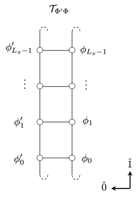
Figure 1: An image of the transfer matrix for the lattice field theory. $\phi^{\prime}_{x}=\phi(t+1,x)$ and $\phi_{x}=\phi(t,x)$ with $x=0,1,2,\cdots,L_{x}-1$. (Note that this figure is not a tensor network representation)

Since ${\cal T}$ is hermitian and positive definite in the model of interest, it has the following eigenvalue decomposition (EVD)

$${\cal T}_{\Phi^{\prime}\Phi}=\sum_{a=0}^{\infty}U_{\Phi^{\prime}a}\lambda_{a}(U^{\dagger})_{a\Phi}\,\,\Longleftrightarrow\,\,\hat{\cal T}|a\rangle=\lambda_{a}|a\rangle$$ (19)

where $U_{\Phi a}=\langle\Phi|a\rangle$ is the unitary matrix composed from the eigenstates and $\lambda_{a}$ are the eigenvalues and assumed to be arranged in descending order, $\lambda_{0}\geq\lambda_{1}\geq\cdots$. The energy gaps defined in eq.(9) may be estimated from the transfer matrix spectrum $\lambda_{a}$ up to lattice cutoff effects

$$\omega_{a}=\ln\left(\frac{\lambda_{0}}{\lambda_{a}}\right)\hskip 14.22636pt\mbox{ for }a=1,2,3,\cdots.$$ (20)

In this way, the diagonalization of the transfer matrix tells us the energy eigenvalues and eigenstates but quantum numbers of each eigenstate are not a priori known, that is, at this stage the correspondence between $(n,q)$ in eq.(3) and $a$ is not clear. To identify the quantum numbers of the eigenstates, an additional procedure is required as follows. First, we have to prepare matrix elements of an interpolating operator $\hat{\cal O}_{q}$ between the energy eigenstates

$$B_{ba}:=\langle b|\hat{\cal O}_{q}|a\rangle=(U^{\dagger}{\cal O}_{q}U)_{ba},$$ (21)

where $U$ is the unitary matrix given in eq.(19) and ${\cal O}_{q}$ is a field representation of the interpolating operator

$$({\cal O}_{q})_{\Phi^{\prime}\Phi}=\langle\Phi^{\prime}|\hat{\cal O}_{q}|\Phi\rangle.$$ (22)

In order to explain how the matrix element is used to determine the quantum number of the eigenstates, let us derive a selection rule for a given symmetry. First, we consider the continuous symmetry case. Let $\hat{Q}$ be a conserved charge associated with the symmetry, and it satisfies $[\hat{Q},\hat{\cal T}]=0$. The associated quantum number (or charge) for some operator $\hat{X}$ is denoted by $q_{X}$,

$$[\hat{Q},\hat{X}]=q_{X}\hat{X}.$$ (23)

Assuming that the ground state has no charge $\hat{Q}|\Omega\rangle=0$, eq.(23) tells us that $\hat{X}|\Omega\rangle$ is an eigenstate of $\hat{Q}$ whose quantum number is $q_{X}$. By sandwiching eq.(23) between $\langle a|$ and $|b\rangle$, one obtains a relationship between the charges and the matrix elements

$$(q_{b}-q_{a}-q_{X})\langle b|\hat{X}|a\rangle=0$$ (24)

where the quantum number of $|a\rangle$ is assumed to be represented as $q_{a}$

$$\hat{Q}|a\rangle=q_{a}|a\rangle.$$ (25)

From eq.(24), we see a selection rule for the continuous symmetry :

for $$\langle b|\hat{X}|a\rangle \neq 0\,\,\,\Longrightarrow\,\,\, q_{b}-q_{a}-q_{X} =0.$$

The selection rule can be used to identify the quantum number of the transfer matrix eigenstates. For example, when we consider eq.(24) with setting $a=0$, which means the ground state and its quantum number is zero $q_{a}=0$, we can say that if the matrix element is $\langle b|\hat{X}|\Omega\rangle\neq 0$ then the quantum number of $|b\rangle$ is shown to be $q_{b}=q_{X}$. In this way, the matrix elements tell us the quantum number of the eigenstates.

Similar argument holds for the discrete symmetry. Let $\hat{D}$ a discrete transformation operator and we assume that the discrete transformation for an operator $\hat{X}$ is given by

$$\hat{D}\hat{X}\hat{D}^{-1}=q_{X}\hat{X}$$ (26)

where we call $q_{X}=\pm 1$ charge of $\hat{X}$ for the discrete symmetry. The ground state is assumed to have the unit charge $\hat{D}|\Omega\rangle=+|\Omega\rangle$. Then by using eq.(26) one can show that $\hat{X}|\Omega\rangle$ is an eigenstate of $\hat{D}$ whose eigenvalue is $q_{X}$, namely, $\hat{D}\hat{X}|\Omega\rangle=q_{X}\hat{X}|\Omega\rangle$. From eq.(26), one can derive a relationship between the charges and the matrix elements

$$\langle b|\hat{X}|a\rangle=\langle b|\hat{D}^{-1}\hat{D}\hat{X}\hat{D}^{-1}\hat{D}|a\rangle=q_{b}q_{a}q_{X}\langle b|\hat{X}|a\rangle,$$ (27)

for the eigenstate $|a\rangle$ whose charge is denoted by $q_{a}$,

$$\hat{D}|a\rangle=q_{a}|a\rangle.$$ (28)

From eq.(27), we read a selection rule for the discrete symmetry :

for $$\langle b|\hat{X}|a\rangle \neq 0 \,\,\,\Longrightarrow\,\,\, q_{b}q_{a}q_{X} =1.$$

As seen in this subsection, the transfer matrix formalism, in principle, can not only obtain the spectrum of a system but also determine the quantum number of the eigenstates. There is, however, a practical difficulty for the formalism. For large lattice volume, the dimension of the transfer matrix becomes extremely large and the numerical computation cannot be done. Thus one has to rely on approximation methods.

2.3 How to compute energy spectrum and matrix elements

As mentioned at the end of the previous subsection, although the transfer matrix formalism is rather theoretically apparent, it is practically very difficult to numerically make the transfer matrix itself for the lattice field theory since the dimensionality of the transfer matrix becomes extremely large. One of way to avoid such a problem is to approximately make the transfer matrix by using the tensor network method. In this case, the dimensionality of the transfer matrix can be drastically reduced and one can numerically treat it as we will see.

The starting point is the definition of the transfer matrix in eq.(14) but here we rewrite it for convenience in the following discussion,

$${\cal T}_{\Phi^{\prime}\Phi} = \left(\prod_{x=0}^{L_{x}-1}\exp\left[-\frac{1}{2}(\phi_{x}^{\prime}-\phi_{x})^{2}-\frac{1}{4}V(\phi^{\prime}_{x})-\frac{1}{4}V(\phi_{x})\right]\right)$$ (29)

$$\times \left(\prod_{x=0}^{L_{x}-1}\exp\left[-\frac{1}{4}(\phi_{x+1}^{\prime}-\phi_{x}^{\prime})^{2}-\frac{1}{8}V(\phi^{\prime}_{x+1})-\frac{1}{8}V(\phi^{\prime}_{x})\right]\right)$$

$$\times \left(\prod_{x=0}^{L_{x}-1}\exp\left[-\frac{1}{4}(\phi_{x+1}-\phi_{x})^{2}-\frac{1}{8}V(\phi_{x+1})-\frac{1}{8}V(\phi_{x})\right]\right),$$

where $\phi^{\prime}_{x}=\phi(t+1,x)$ and $\phi_{x}=\phi(t,x)$ with $x=0,1,2,\cdots,L_{x}-1$. The first term represents a hopping for the time direction. The second and third terms are for the space direction at the time slice $t+1$ and $t$ respectively. If we apply the eigenvalue decomposition (EVD) to each local Boltzmann weight for the time hopping in eq.(29),

$$\exp\left[-\frac{1}{2}(\phi_{x}^{\prime}-\phi_{x})^{2}-\frac{1}{4}V(\phi^{\prime}_{x})-\frac{1}{4}V(\phi_{x})\right]=\sum_{k_{x}=0}^{\infty}u_{\phi^{\prime}_{x}{k_{x}}}\sigma_{k_{x}}(u^{\dagger})_{k_{x}\phi_{x}},$$ (30)

then we can decompose the transfer matrix as follows

$${\cal T}_{\Phi^{\prime}\Phi}=\sum_{k}Y_{\Phi^{\prime}k}Y^{\dagger}_{k\Phi},$$ (31)

with

$$Y_{\Phi k} = \left(\prod_{x=0}^{L_{x}-1}\sum_{k_{x}=0}^{\infty}u_{\phi_{x}{k_{x}}}\sqrt{\sigma_{k_{x}}}\right)$$ (32)

$$\times \left(\prod_{x=0}^{L_{x}-1}\exp\left[-\frac{1}{4}(\phi_{x+1}-\phi_{x})^{2}-\frac{1}{8}V(\phi_{x+1})-\frac{1}{8}V(\phi_{x})\right]\right),$$

where we have defined the integrated index, $k=(k_{0},k_{1},k_{2},\cdots,k_{L_{x}-1})$. An image of the decomposition in eq.(31) is shown in Fig. 2.

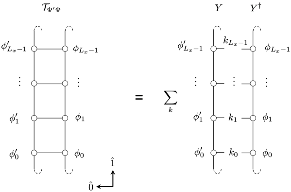
Figure 2: Graphical expression of the decomposition of the transfer matrix in terms of $Y$ in eq.(31). (Note that this figure is not a tensor network representation)

Figure 3: The definition of ${\cal A}$ in eq.(34) and its tensor network representation in terms of the local tensor $A$ in eq.(36).

Substituing the transfer matrix in eq.(31) into the partition function, we obtain

$$Z={\rm Tr}_{\Phi}\left[{\cal T}^{L_{\tau}}\right]={\rm Tr}_{\Phi}\left[(YY^{\dagger})^{L_{\tau}}\right]={\rm Tr}_{k}\left[(Y^{\dagger}Y)^{L_{\tau}}\right]={\rm Tr}_{k}\left[{\cal A}^{L_{\tau}}\right],$$ (33)

where in the last equal we have defined

$${\cal A}:=Y^{\dagger}Y.$$ (34)

Note that the ordering of $Y$ and $Y^{\dagger}$ is different in ${\cal T}$ and ${\cal A}$. As shown in Fig. 3, actually ${\cal A}$ can be simply expressed by a tensor network representation

$${\cal A}_{kj} = \sum_{\Phi}(Y^{\dagger})_{k\Phi}Y_{\Phi j}$$ (35)

$$= \sum_{\Phi}\left(\prod_{x=0}^{L_{x}-1}\sum_{k_{x}=0}^{\infty}(u^{\dagger})_{k_{x}\phi_{x}}\sqrt{\sigma_{k_{x}}}\right)\left(\prod_{x=0}^{L_{x}-1}\sum_{j_{x}=0}^{\infty}u_{\phi_{x}{j_{x}}}\sqrt{\sigma_{j_{x}}}\right)$$

$$\times \left(\prod_{x=0}^{L_{x}-1}\exp\left[-\frac{1}{2}(\phi_{x+1}-\phi_{x})^{2}-\frac{1}{4}V(\phi_{x+1})-\frac{1}{4}V(\phi_{x})\right]\right)$$

$$= \prod_{x=0}^{L_{x}-1}\sum_{l_{x}=0}^{\infty}A_{k_{x}l_{x}j_{x}l_{x-1}}$$

with a rank-4 tensor $A$

$$A_{k_{x}l_{x}j_{x}l_{x-1}}:=\sqrt{\sigma_{k_{x}}\sigma_{l_{x}}\sigma_{j_{x}}\sigma_{l_{x-1}}}\sum_{\phi_{x}}(u^{\dagger})_{k_{x}\phi_{x}}(u^{\dagger})_{l_{x}\phi_{x}}u_{\phi_{x}j_{x}}u_{\phi_{x}l_{x-1}}.$$ (36)

When deriving the initial tensor $A$, we have applied the EVD to the spatial hopping terms in eq.(35)

$$\exp\left[-\frac{1}{2}(\phi_{x+1}-\phi_{x})^{2}-\frac{1}{4}V(\phi_{x+1})-\frac{1}{4}V(\phi_{x})\right]=\sum_{l_{x}=0}^{\infty}u_{\phi_{x+1}{l_{x}}}\sigma_{l_{x}}(u^{\dagger})_{l_{x}\phi_{x}},$$ (37)

for $x\in\{0,1,2,\cdots,L_{x}-1\}$.

Note that singular value decomposition (SVD) of $Y$ is given by

$$Y=U\sqrt{\lambda}W^{\dagger}$$ (38)

where $U$ and $\lambda$ are the same as those of the transfer matrix ${\cal T}$ in eq.(19). On the other hand, the EVD for ${\cal A}$ is given by

$${\cal A}=Y^{\dagger}Y=W\lambda W^{\dagger},$$ (39)

thus ${\cal A}$ has the same eigenvalues as those of ${\cal T}$.

From here let us explain how to numerically compute the spectrum by using the tensor network method [47]. First we coarse-grain the tensor network consisted of the initial tensor $A$ in eq.(36) on the square lattice with $L_{\tau}=L_{x}=2^{n}$ by using HOTRG [50] as shown in Fig. 4,

$$A=A^{[0]}\stackrel{{\scriptstyle{\rm HOTRG}}}{{\longrightarrow}}A^{[1]}\stackrel{{\scriptstyle{\rm HOTRG}}}{{\longrightarrow}}A^{[2]}\stackrel{{\scriptstyle{\rm HOTRG}}}{{\longrightarrow}}\cdots.$$ (40)

and then after $n-1$ iterations, one arrives at four renormalized tensors $A^{[n-1]}$. Subsequently we perform the direct contraction of those tensors taking into account the periodic boundary condition on the spatial direction, and we obtain a numerical approximation of a power of ${\cal A}$ as follows

$${\cal A}^{L_{\tau}}\approx{\mathcal{A}}^{[n]}_{k_{1}k_{2},j_{1}j_{2}}=\sum_{l_{1},l_{2},m_{1},m_{2},n_{1},n_{2}}A^{[n-1]}_{k_{1}l_{1}n_{1}l_{2}}A^{[n-1]}_{k_{2}l_{2}n_{2}l_{1}}A^{[n-1]}_{n_{1}m_{1}j_{1}m_{2}}A^{[n-1]}_{n_{2}m_{2}j_{2}m_{1}}.$$ (41)

Subsequently, we diagonalize $\mathcal{A}^{[n]}$ as follows,

$$\mathcal{A}^{[n]}=W^{[n]}\lambda^{[n]}W^{[n]\dagger}$$ (42)

where $W^{[n]}$ is unitary matrix containing numerical eigenvectors, and $\lambda^{[n]}$ is the eigenvalues. Note that the original lattice size in the time direction of ${\cal A}^{[n]}$ is $L_{\tau}(=2^{n})$, thus the tensor network estimation of the transfer matrix eigenvalue is given by

$$\lambda_{a}\approx\left(\lambda_{a}^{[n]}\right)^{1/L_{\tau}}$$ (43)

then the energy gap is estimated as

$$\omega_{a}\approx\frac{1}{L_{\tau}}\log\left(\frac{\lambda_{0}^{[n]}}{\lambda_{a}^{[n]}}\right)=:\omega_{a}^{[{\rm hotrg}]}\,\,\,\,\mbox{ for }a=1,2,3,\cdots.$$ (44)

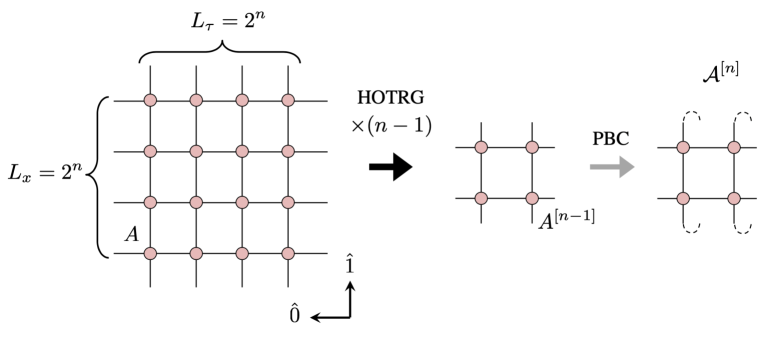
Figure 4: The black arrow shows the coarse-graining procedure of the tensor network. The procedure is done until there are only four ${A}^{[n-1]}$s. The gray arrow shows the direct contraction of the last four tensors to obtain the approximation of ${\cal A}^{L_{\tau}}\approx{\cal A}^{[n]}$. Here the PBC is imposed on the space direction.

Next, let us see how to compute the matrix elements by the tensor network method. For that purpose, first we rewrite the matrix elements in eq.(21) in terms of the tensor network related quantities. For an integer $m=L_{\tau}/2$ (assuming that $L_{\tau}$ is even number), the matrix elements may be expressed as follows,

$$B_{ba} = \langle b|\hat{\cal O}_{q}|a\rangle=(U^{\dagger}{\cal O}_{q}U)_{ba}$$ (45)

$$= (U^{\dagger}{\cal T}^{-m}{\cal T}^{m}{\cal O}_{q}{\cal T}^{m+1}{\cal T}^{-(m+1)}U)_{ba}\,\,\,(\because{\cal T}{\cal T}^{-1}=1)$$

$$= (U^{\dagger}(U\lambda U^{\dagger})^{-m}(YY^{\dagger})^{m}{\cal O}_{q}(YY^{\dagger})^{m+1}(U\lambda U^{\dagger})^{-(m+1)}U)_{ba}\,\,\,(\because\mbox{eq.(\ref{eqn:T_EVD}) and eq.(\ref{eqn:TM_YY})})$$

$$= (\lambda^{-m}U^{\dagger}Y(Y^{\dagger}Y)^{m-1}Y^{\dagger}{\cal O}_{q}Y(Y^{\dagger}Y)^{m}Y^{\dagger}U\lambda^{-(m+1)})_{ba}$$

$$= (\lambda^{-m}U^{\dagger}Y{\cal A}^{m-1}{\cal A}^{\prime}{\cal A}^{m}Y^{\dagger}U\lambda^{-(m+1)})_{ba}\,\,\,(\because\mbox{eq.(\ref{eqn:tildeT_YY}) and }{\cal A}^{\prime}:=Y^{\dagger}{\cal O}_{q}Y)$$

$$= (\lambda^{-m+1/2}W^{\dagger}{\cal A}^{m-1}{\cal A}^{\prime}{\cal A}^{m}W\lambda^{-m-1/2})_{ba}\,\,\,(\because\mbox{eq.(\ref{eqn:Y_SVD})})$$

where we have defined an impurity version of ${\cal A}$, that is, ${\cal A}^{\prime}:=Y^{\dagger}{\cal O}_{q}Y$ and an impurity tensor network ${\cal A}^{m-1}{\cal A}^{\prime}{\cal A}^{m}$ as shown in Fig. 5. Here we assume that the lattice size for the impurity tensor network is the same as that of pure tensor network $L_{\tau}=L_{x}=2^{n}$. If we consider a single field ${\cal O}_{q}=\phi_{x}$ at a lattice site $x$, then the associated impurity tensor $A^{\prime}$ is given by

$$A_{k_{x}l_{x}j_{x}l_{x-1}}^{\prime}:=\sqrt{\sigma_{k_{x}}\sigma_{l_{x}}\sigma_{j_{x}}\sigma_{l_{x-1}}}\sum_{\phi_{x}}\phi_{x}(u^{\dagger})_{k_{x}\phi_{x}}(u^{\dagger})_{l_{x}\phi_{x}}u_{\phi_{x}j_{x}}u_{\phi_{x}l_{x-1}}.$$ (46)

In this way, one can represent the matrix elements in terms of the impurity tensor network ${\cal A}^{m-1}{\cal A}^{\prime}{\cal A}^{m}$, $W$ and $\lambda$ that are obtained from the EVD of ${\cal A}$ as in eq.(39).

In order to numerically evaluate the impurity tensor network ${\cal A}^{m-1}{\cal A}^{\prime}{\cal A}^{m}$, we apply the coarse-graining procedure to this network using the same isometries as in the pure tensor network coarse-graining steps shown in Fig. 4 until there are four tensors. We denote the coarse-grained impurity tensor network ($2\times 2$ network in Fig. 5) as ${\cal A}^{\prime[n]}$,

$${\cal A}^{m-1}{\cal A}^{\prime}{\cal A}^{m}\approx{\cal A}^{\prime[n]}.$$ (47)

Some readers may wonder why we choose $m=L_{\tau}/2$ but not like $1$ or some small value that means cheap computational cost. In such a small $m$ case, however, we find that an accuracy of the evaluation of the impurity tensor network turns out to be worse. On the other hand, for $m=L_{\tau}/2$ in eq.(47) that corresponds to the square impurity tensor network, the coarse-graining procedure is rather simple and we find that the accuracy is reasonably maintained during the coarse-graining, thus we choose this value of $m$. By using ${\cal A}^{\prime[n]}$ in eq.(47), $W^{[n]}$ and $\lambda^{[n]}$ in eq.(42), the matrix elements in eq.(45) may be estimated by

$$B_{ba}\approx\left(\lambda^{[n]}\right)^{-\frac{L_{\tau}-1}{2L_{\tau}}}W^{[n]{\dagger}}{\cal A}^{\prime[n]}W^{[n]}\left(\lambda^{[n]}\right)^{-\frac{L_{\tau}+1}{2L_{\tau}}}=:B_{ba}^{[{\rm hotrg}]}.$$ (48)

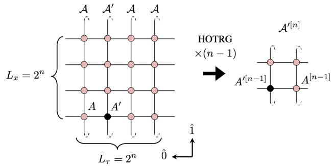
Figure 5: The coarse-graining procedure of the impurity tensor network ${\cal A}^{m-1}{\cal A}^{\prime}{\cal A}^{m}$ with the single field operator ${\cal O}_{q}=\phi_{x}$. The procedure is done until there are four tensors.

3 Numerical Results

In this section, we demonstrate our scheme by applying it to $(1+1)$d Ising model with zero external magnetic field and the periodic boundary condition. The details for the model, say its transfer matrix and tensor network representation are given in Appendix A. We will show that the scheme can produce the energy spectrum of the model and the result will be compared with the exact spectrum [64] summarized in Appendix B. The matrix elements for the model with a single spin field or double fields are also computed to judge the quantum number of the eigenstates. Furthermore the wave function of the eigenstates and the scattering phase shift are computed as well.

3.1 Energy spectrum

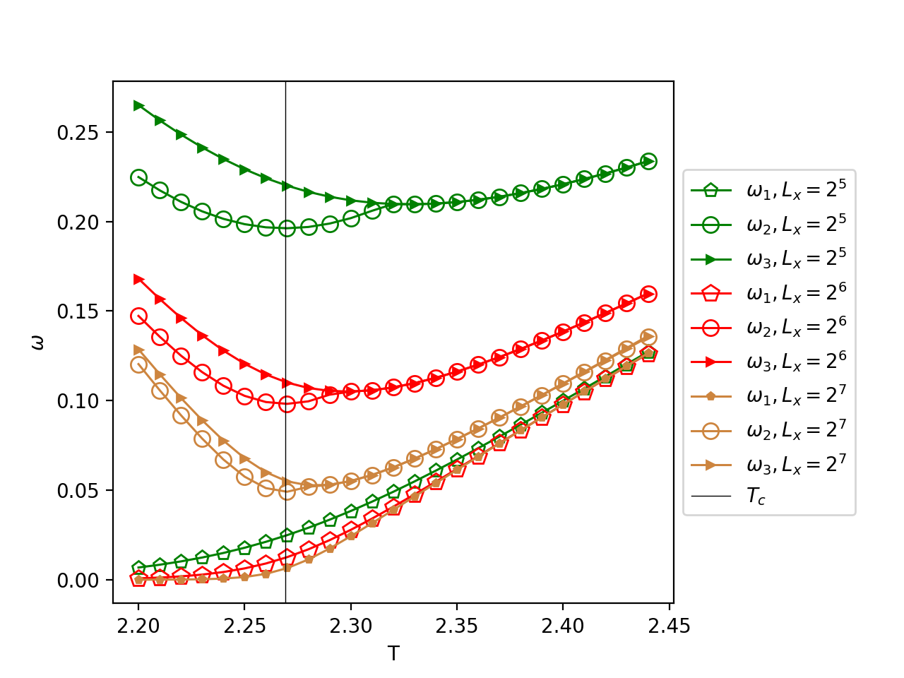
(a)

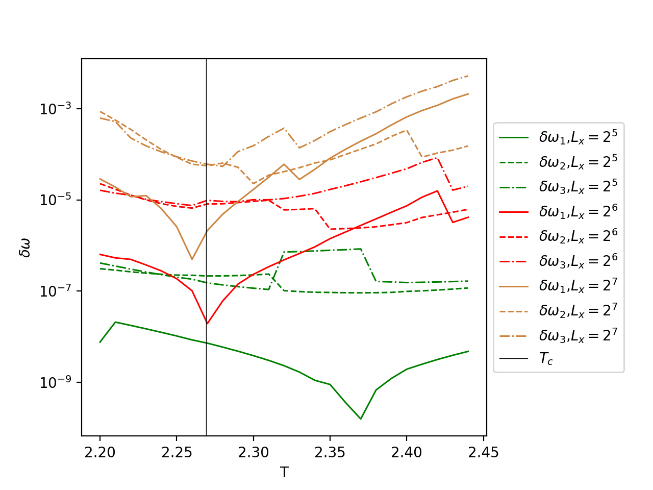
(b)

Figure 6: (a) Three lowest energy gaps $\omega_{a}$ ($a=1,2,3$) for system size $L_{x}=2^{5},2^{6},2^{7}$ around the critical temperature $T_{\rm c}$ with $\chi=80$. (b) The relative error of the energy gap $\delta\omega_{a}$ .

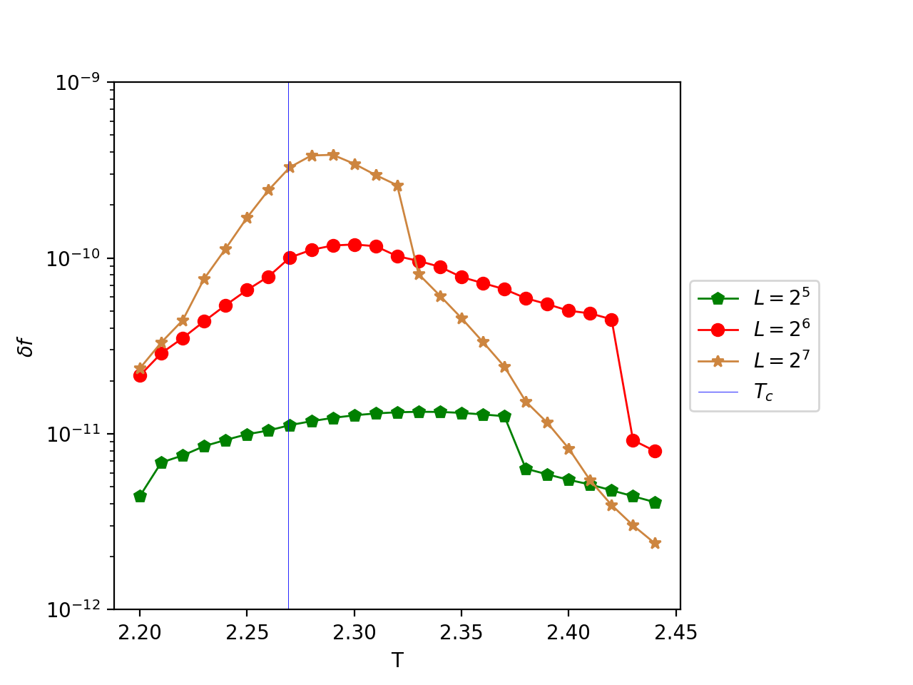
Figure 7: The relative error of the free energy $\delta f$ at finite volume $V=L^{2}$ with $L=L_{x}=L_{\tau}$ computed by HOTRG with $\chi=80$. Around the critical point, $\delta f$ has a peak in contrast to $\delta\omega_{1}$ in Fig. 6(b).

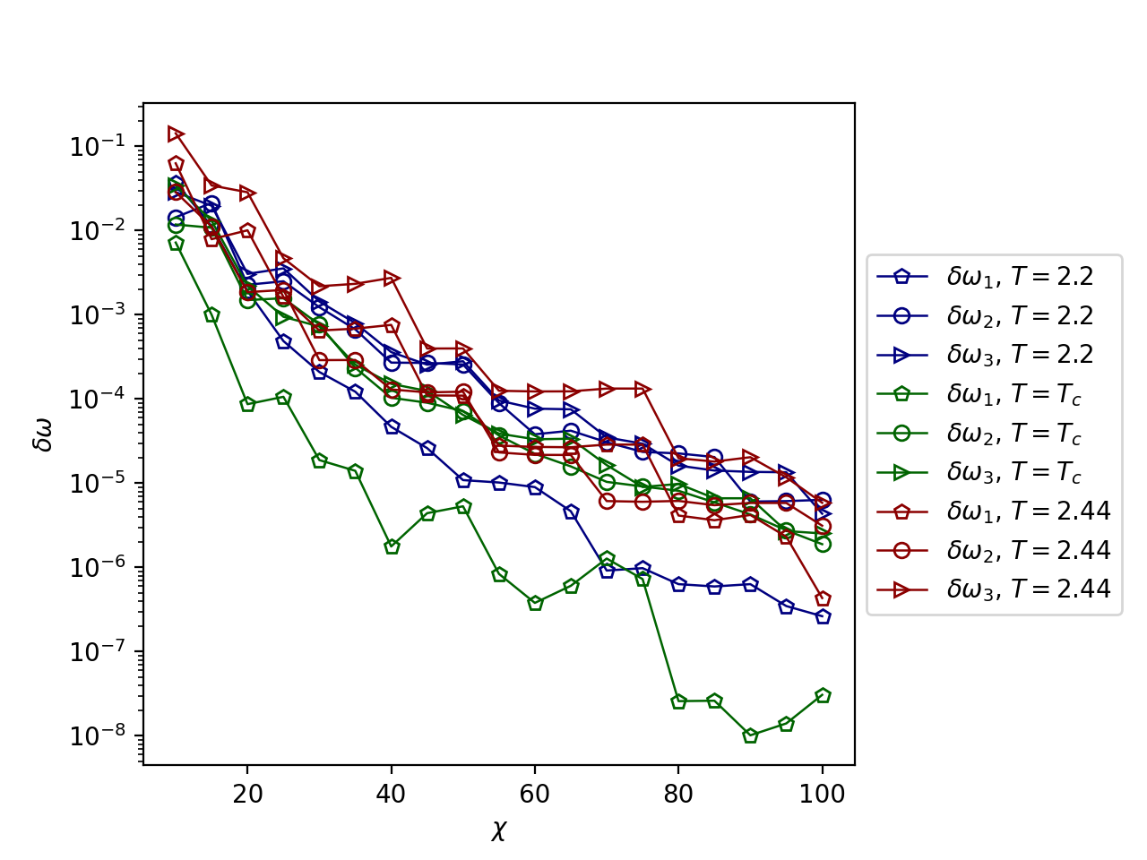
Figure 8: The relative error of the three lowest energy gaps at three different temperatures $T=2.2,T_{\rm c},2.44$ with $L_{x}=2^{6}$ as a function of the bond dimension $\chi$.

According to Sec. 2.3, we compute the energy gaps $\omega_{a}^{[{\rm hotrg}]}$ in eq.(44) using HOTRG with a given bond dimension $\chi$. Figure 6(a) shows the three lowest energy gaps in the temperature range $T=2.2-2.44$ encompassing the critical point $T_{\rm c}=\frac{2}{\log(1+\sqrt{2})}$ for system size $L_{x}=2^{5}-2^{7}$ with $\chi=80$. We observe an expected behavior; by increasing the system size the lowest gap $\omega_{1}$ below $T_{\rm c}$ tends to be close to zero while it stays nonzero for the temperature above $T_{\rm c}$. In order to see an accuracy of the energy gap, we show its relative error

$$\delta\omega_{a}=\left|\frac{\omega_{a}^{[\text{exact}]}-\omega_{a}^{[\text{hotrg}]}}{\omega_{a}^{[\text{exact}]}}\right|$$ (49)

in Fig. 6(b). Here $\omega^{[\text{exact}]}_{a}$ is the Kaufman’s exact results for finite volume [64] (see Appendix B for details). From this figure, we can see that the relative error increases for larger system size due to the iteration of the coarse-graining step. We also observe that $\delta\omega_{1}$ apparently has a minimum around the critical point while $\delta\omega_{2}$ and $\delta\omega_{3}$ do not show such a behavior. We note that the behavior of $\delta\omega_{1}$ is in contrast with the relative error of the free energy at finite volume

$$\delta f=\left|\frac{f^{\text{[exact]}}_{V}-f^{[\text{hotrg}]}_{V}}{f^{[\text{exact}]}_{V}}\right|$$ (50)

where $f^{[\text{exact}]}_{V}$ is the exact free energy with volume $V=L^{2}$ with $L=L_{x}=L_{\tau}$ [64]. The relative error $\delta f$ is shown in Fig. 7 where the error becomes large around the critical point.

Next, let us see how the relative error of the energy gap scales with the bond dimension. Figure 8 shows $\delta\omega_{a}$ $(a=1,2,3)$ as a function of $\chi$ for selected values of the temperature. From this figure, we can see that for all cases, the relative error tends to decrease when increasing the bond dimension.

3.2 Quantum number classification

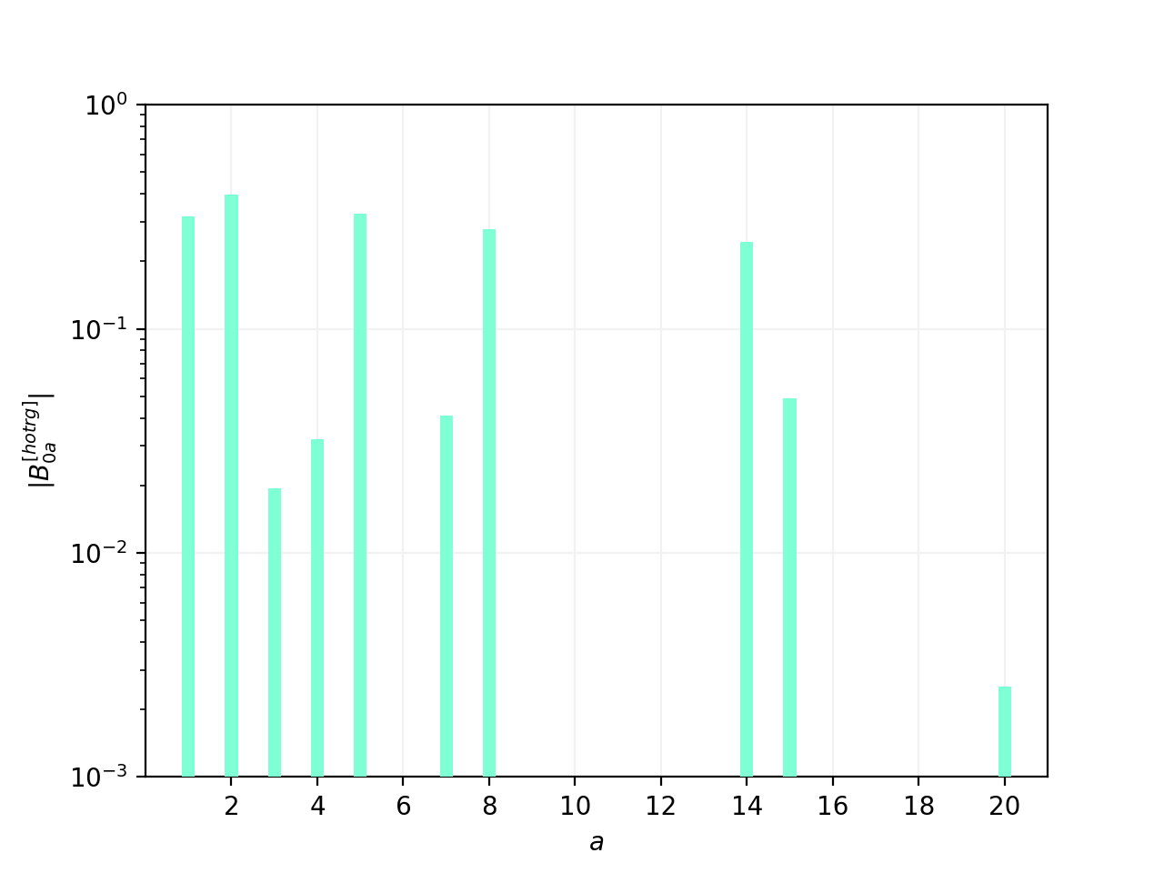
Figure 9: The matrix element $B_{0a}^{[\text{hotrg}]}$ for $a=1,2,3,\cdots,20$ at $T=2.44$ with $L_{x}=2^{6}$ and $\chi=80$.

Table 1: Comparison to the exact result for $T=2.44$ and $L_{x}=2^{6}$. $\delta\omega_{a}$ is the relative error of the energy gap defined in eq.(49). The momentum $p$ is diagnosed in Sec. 3.3.

$a$	$\omega_{a}^{[{\rm exact}]}$	$q_{a}$	$\omega_{a}^{[{\rm hotrg}]}$	$q_{a}$	$\delta\omega_{a}$	$|p|$
1	0.1262302	$-$	0.1262307	$-$	0.000004	$0$
2	0.1597880	$-$	0.1597889	$-$	0.000006	$2\pi/L_{x}$
3	0.1597880	$-$	0.1597911	$-$	0.000020	$2\pi/L_{x}$
4	0.2326853	$-$	0.2327046	$-$	0.000083	$4\pi/L_{x}$
5	0.2326853	$-$	0.2327095	$-$	0.000104	$4\pi/L_{x}$
6	0.2708016	$+$	0.2708359	$+$	0.000127	$*$
7	0.3181546	$-$	0.3183329	$-$	0.000560	$6\pi/L_{x}$
8	0.3181546	$-$	0.3183705	$-$	0.000679	$6\pi/L_{x}$
9	0.3290037	$+$	0.3291180	$+$	0.000347	$*$
10	0.3290037	$+$	0.3291425	$+$	0.000422	$*$
11	0.3290037	$+$	0.3291456	$+$	0.000431	$*$
12	0.3290037	$+$	0.3293794	$+$	0.001142	$*$
13	0.3872058	$+$	0.3878486	$+$	0.001660	$*$
14	0.4073042	$-$	0.4083937	$-$	0.002675	$8\pi/L_{x}$
15	0.4073042	$-$	0.4090231	$-$	0.004220	$8\pi/L_{x}$
16	0.4100181	$+$	0.4109090	$+$	0.002173	$*$
17	0.4100181	$+$	0.4112006	$+$	0.002884	$*$
18	0.4100181	$+$	0.4112120	$+$	0.002912	$*$
19	0.4100181	$+$	0.4114574	$+$	0.003510	$*$
20	0.4457831	$-$	0.4461242	$-$	0.000765	$0$

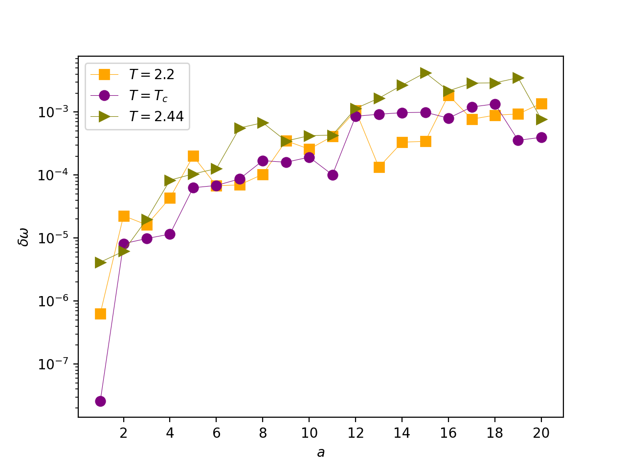
Figure 10: The relative error of the energy gap $\delta\omega_{a}$ for $a=1,2,3,\cdots,20$ at three different temperature cases: $T=2.2$, $T_{c}$ and $2.44$. The system size is $L_{x}=2^{6}$ and the bond dimension is $\chi=80$.

The Ising model with zero external magnetic field has $Z_{2}$ symmetry, thus the energy eigenstates are divided into two groups labeled by the quantum number $q=\{+1,-1\}$. In order to determine the quantum number of the eigenstates, following the procedure described in Sec. 2.3 we compute the matrix elements $B_{ba}^{[\text{hotrg}]}$ in eq.(48) with a proper interpolation operator. Here we choose the simplest choice i.e. a single spin field $\mathcal{O}_{q}=s_{x}$ ($=s_{0}$ at $x=0$) whose quantum number is $q=-1$.

Once the elements of $B_{ba}^{[\text{hotrg}]}$ are estimated, the quantum number of the eigenstate can be determined from the selection rule as discussed in Sec. 2.2. Since the ground state ($a=0$) has quantum number $q=+1$, we can classify the quantum number of the rest of the states labeled with $a=1,2,3,\cdots,$ by only looking at the first row of the estimated matrix $B_{0a}^{[\text{hotrg}]}\approx\langle\Omega|s_{0}|a\rangle$. The selection rule tells us the quantum number of $|a\rangle$, $q_{a}$ as follows. For each $a$,

$$\mbox{ if }B_{0a}^{[\text{hotrg}]}\neq 0 \Longrightarrow q_{a}=-1,$$ (51)

$$\mbox{ if }B_{0a}^{[\text{hotrg}]}=0 \Longrightarrow q_{a}=+1.$$ (52)

See Fig. 9 for the result of $B_{0a}^{[\text{hotrg}]}$ for $a=1,2,3,\cdots,20$ at $T=2.44$, $L_{x}=2^{6}$ and $\chi=80$. The judged result of $q_{a}$ is listed in Table 1 together with the exact one obtained from Appendix B. As a result, the quantum number is correctly judged up to 20 eigenstates for this parameter set. On the other hand, for eigenstates with $a>20$, our scheme fails to reproduce the correct quantum number although we do not show them here. In fact, it is difficult not only to judge the quantum number but also to obtain accurate energy gaps for higher excited states as seen in Table 1 (column for $\delta\omega_{a}$) and Fig. 10 where the relative error of the energy gap for $T=2.2$, $T_{\rm c}$ and $2.44$ tends to be large for larger $a$.

3.3 Momentum identification

On a finite spatial volume, the momentum is discretized as $p=2\pi k/L_{x}$ with $k=0,1,2,\cdots,L_{x}-1$ (or equivalently $k=-L_{x}/2+1,-L_{x}/2+2,\cdots,-1,0,1,\cdots,L_{x}/2-1,L_{x}/2$ assuming that $L_{x}$ is even number), and the momentum of the single particle state can also be determined as follows.

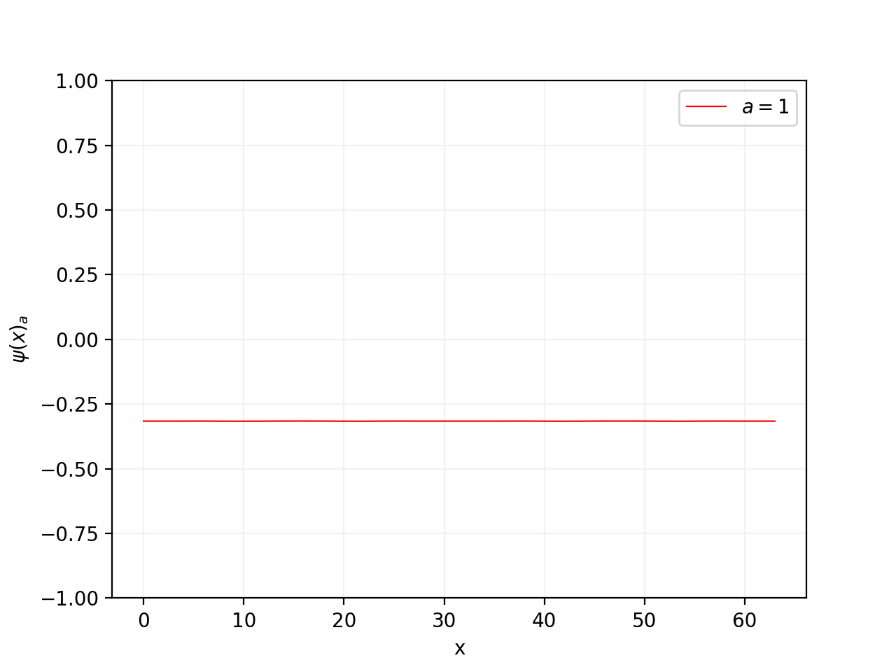
(a)

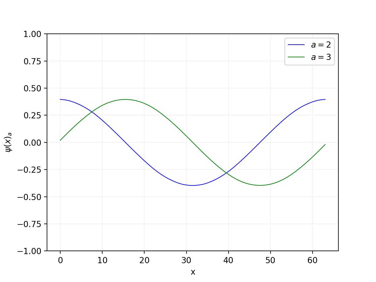
(b)

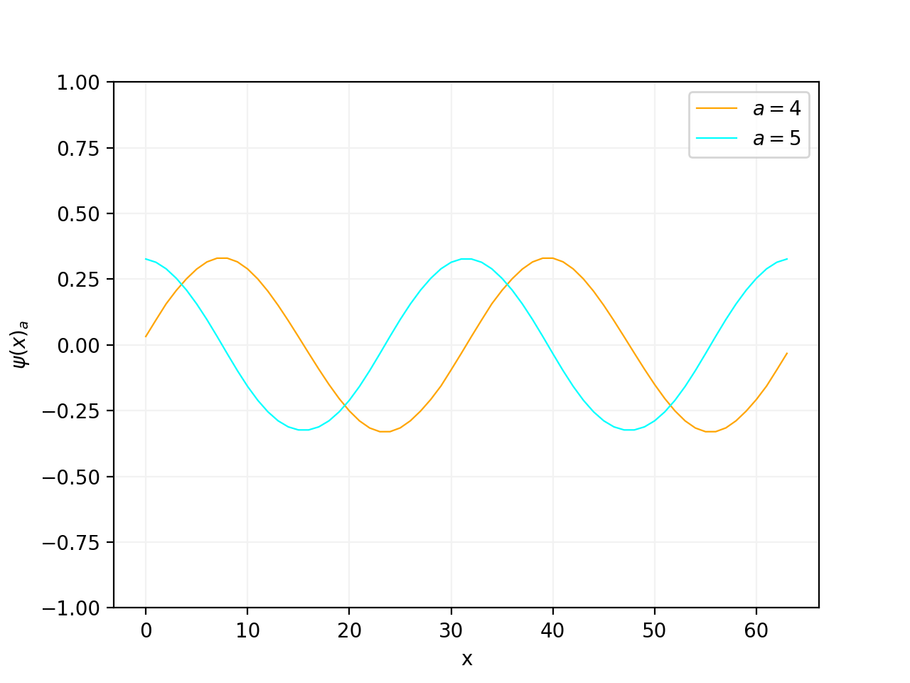
(c)

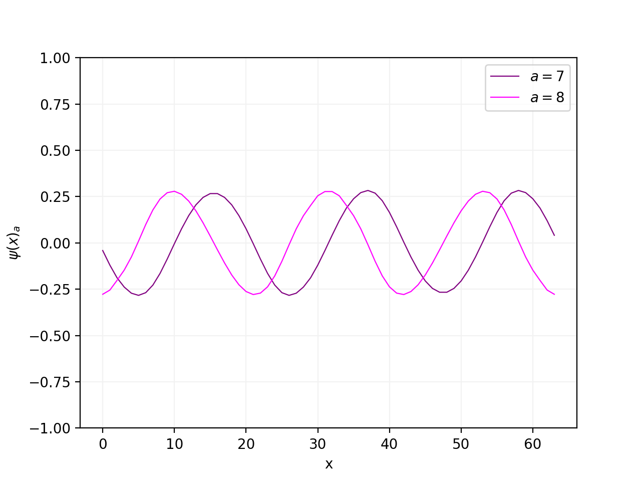
(d)

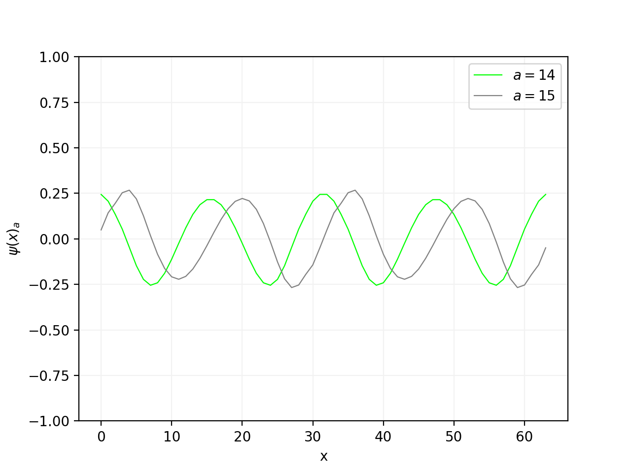
(e)

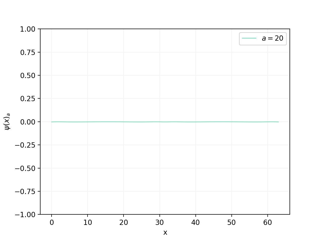
(f)

Figure 11: The wave function of the eigenstates for $q=-1$ sector with $T=2.44$ and $L_{x}=2^{6}$ computed by HOTRG with $\chi=80$.

A simple way to check (the absolute value of) the momentum of a single particle state for $q=-1$ sector is to look at its wave function in position space

$$\psi_{a}(x)=\langle\Omega|s_{x}|a\rangle,$$ (53)

where $s_{x}$ is the spin field at $x=0,1,2,\cdots,L_{x}-1$. The computation of the wave function can be done in a similar way to the matrix element $B_{0a}^{[\text{hotrg}]}$ given in the previous subsection, but now we have to repeat it for all possible values of $x$. Figure 11 shows the numerical results of the wave functions for $q=-1$ sector ($a=1,2,3,4,5,7,8,14,15,20$) with $T=2.44$, $L_{x}=2^{6}$ and $\chi=80$. The wave function data is well described by functional form

$$\psi_{a}(x)\propto\cos\left[p\left(x+\frac{1}{2}\right)\right]\mbox{ or }\sin\left[p\left(x+\frac{1}{2}\right)\right]$$ (54)

where $p=2\pi k/L_{x}$ is the discrete momentum. For example, $a=1$ state in Fig. 11(a) shows constant behavior thus this is apparently zero momentum state. The states for $a=2$ and $3$ (see Fig. 11(b)) are described by

$$\psi_{2}(x)\propto\cos\left[p\left(x+\frac{1}{2}\right)\right]\mbox{ and }\psi_{3}(x)\propto\sin\left[p\left(x+\frac{1}{2}\right)\right]\mbox{ with }p=\frac{2\pi}{L_{x}},$$ (55)

therefore the momentum of those states are judged to be $|p|=2\pi/L_{x}$. The same thing can be applied to other states ($a=4,5$ states are paired and they correspond to momentum $4\pi/L_{x}$ and so on), and the resulting momentum is summarized in Table 1. One thing to be noted is that, the wave function for $a=20$ in Fig. 11(f) seems to have zero amplitude over all $x$ at this scale of the $y$-axis, but in fact it has non-zero amplitude of order $O(10^{-3})$ as seen in Fig. 9, where $\psi_{20}(0)$ is plotted, therefore this is considered as a first excited state for the zero momentum channel. The smallness of the amplitude simply reflects the small overlap of this state with the single spin field.

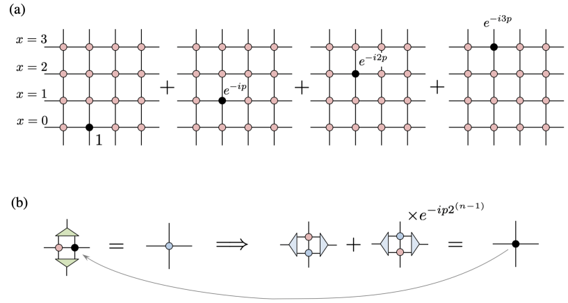
Figure 12: (a) Tensor network presentation with the impurity tensor for the single field in the momentum space $s_{p}=\frac{1}{L_{x}}\sum_{x}s_{x}e^{-ipx}$. The black points represent the impurity tensor $A^{\prime}\times e^{-ipx}$ where $A^{\prime}$ is defined in eq.(46). (b) A coarse-graining procedure for the tensor network of (a). Here 3-leg tensors represent the isometry for HOTRG and $n$ is the number of coarse-graining steps ($n=1,2,3,\cdots$).

To quantitatively confirm the momentum identification presented in the previous paragraph, we compute the matrix elements with a proper momentum field. From the Fourier transformation of the spin field

$$s_{p}=\frac{1}{L_{x}}\sum_{x=0}^{L_{x}-1}s_{x}e^{-ipx}$$ (56)

where the momentum is discretized $p=2\pi k/L_{x}$, one can define matrix elements

$$\langle\Omega|s_{p}|a\rangle=\frac{1}{L_{x}}\sum_{x}\langle\Omega|s_{x}|a\rangle e^{-ipx}.$$ (57)

Using the matrix elements together with the selection rule, we can see that for given $a$ (in $q=-1$ sector) and $p$,

$$\langle\Omega|s_{p}|a\rangle\neq 0\Longrightarrow|a\rangle\mbox{ belongs to }|p|\mbox{ sector}.$$ (58)

In this way, the momentum of $|a\rangle$ can be identified. The matrix elements in eq.(57) can be efficiently computed as shown in Fig. 12 following the idea in [75]. Table 2 shows numerical results of the matrix element for $T=2.44$ and $L_{x}=2^{6}$. In order to see the bond dimension dependence, we use $\chi=70,80,100$. For example, we can see that the momentum of $a=1$ and $20$ states is $p=0$, and for $a=2$ and $3$, their momentum is $|p|=2\pi/L_{x}$, and so on. We note that some states develop fake nonzero matrix elements due to the truncation error in the coarse-graining step. We can, however, eliminate such a fake behavior by increasing the bond dimension. For example, $a=20$ state has the nonzero matrix elements for $p=0,4\pi/L_{x},8\pi/L_{x}$, but the values for $p=4\pi/L_{x}$ and $8\pi/L_{x}$ tend to be small for larger $\chi$. Thus we conclude that $a=20$ state belongs to the zero momentum.

Table 2: The absolute value of the matrix elements $|\langle\Omega|s_{p}|a\rangle|$ for $T=2.44$ and $L_{x}=2^{6}$ using $\chi=70,80,100$. Here we show only nonzero values that are larger than $O(10^{-5})$. For the shaded case, the associated matrix elements are judged to be consistent with zero since their values are small and they tend to be small for large $\chi$.

$k$	$|p|$	$a$	$\chi=70$	$\chi=80$	$\chi=100$
0	0	$1$	$0.31608$	$0.31609$	$0.31610$
		$20$	$0.00195$	$0.00200$	$0.00208$
1	$2\pi/L_{x}$	$2$	$0.19850$	$0.19850$	$0.19850$
		$3$	$0.19844$	$0.19849$	$0.19850$
2	$4\pi/L_{x}$	$4$	$0.16406$	$0.16406$	$0.16409$
		$5$	$0.16370$	$0.16404$	$0.16406$
		$1$	$0.00012$	$0.00002$	$<10^{-5}$
		$14$	$0.00001$	$<10^{-5}$	$<10^{-5}$
		$20$	$0.00021$	$0.00017$	$0.00012$
3	$6\pi/L_{x}$	$7$	$0.13934$	$0.13940$	$0.13967$
		$8$	$0.13750$	$0.13932$	$0.13932$
		$2$	$0.00006$	$0.00006$	$0.00002$
		$3$	$0.00061$	$0.00010$	$0.00006$
4	$8\pi/L_{x}$	$14$	$0.12013$	$0.12104$	$0.12201$
		$15$	$<10^{-5}$	$0.12011$	$0.12012$
		$1$	$0.00043$	$0.00006$	$0.00001$
		$4$	$0.00057$	$0.00059$	$0.00017$
		$5$	$0.00304$	$0.00052$	$0.00059$
		$19$	$0.11386$	$<10^{-5}$	$<10^{-5}$
		$20$	$0.00022$	$0.00035$	$0.00016$

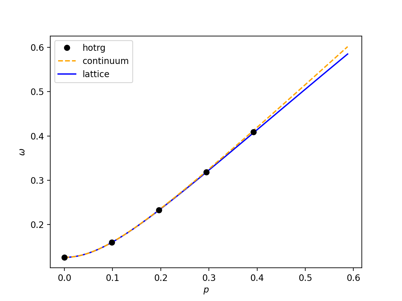
Figure 13: The dispersion relation for the single particle of $(1+1)$d Ising model at $T=2.44$ with $L_{x}=2^{6}$. The circle is the energy gap at the corresponding momentum computed by HOTRG with $\chi=80$. The dashed line is continuum dispersion relation in eq.(59) while the solid line is the lattice version in eq.(60).

As seen in the previous paragraph, the momentum is determined thus now we can check the dispersion relation between the energy and the momentum. As seen in Table 1, the degeneracy of the energy for the non-zero momentum with $q=-1$ is slightly broken due to the truncation error, therefore we use an average of them as the energy $\omega$. See Fig. 13 for the dispersion relation with $T=2.44$ and $L_{x}=2^{6}$. The data points are generated by HOTRG with $\chi=80$ and compared with the continuum version of the dispersion relation

$$\omega=\sqrt{m^{2}+p^{2}}$$ (59)

and the lattice version [66]

$$\omega=\operatorname{arccosh}(1-\cos p+\cosh m)$$ (60)

where $m$ is the rest mass. Both cases describe the data well and the lattice version is slightly better especially for higher momentum region.

3.4 Scattering phase shift

In order to study the two-particle channel ($q=+1$ sector), we consider two-field operators

$${\cal O}_{2}(P,p)=\frac{1}{L_{x}^{2}}\sum_{x,y=0}^{L_{x}-1}s_{x}s_{y}e^{-ip_{1}x-ip_{2}y}$$ (61)

where $p_{1}$ and $p_{2}$ are the discrete momentum $p_{j}=2\pi n_{j}/L_{x}$ with $n_{j}\in\mathbb{Z}$ ($j=1,2$), and the total momentum $P$ and the relative one $p$ are given by

$$P = p_{1}+p_{2},$$ (62)

$$p = \frac{1}{2}(p_{1}-p_{2}).$$ (63)

The matrix elements of the operators

$$\langle\Omega|{\cal O}_{2}(P,p)|a\rangle$$ (64)

are useful to identify the momentum for the states with $q=+1$ sector. For example, for a given value of $P$, if the matrix element has a nonzero value

$$\langle\Omega|{\cal O}_{2}(P,p)|a\rangle\neq 0,$$ (65)

then the total momentum of $|a\rangle$ is estimated to be $P$ irrespective of $p$. A tensor network representation with the impurity tensors for the two-field operator with $L_{x}=4$ is shown in Fig. 14 where its computational procedure is also described.

Figure 14: (a)Tensor network presentation with the impurity tensors for the operator $\hat{\cal O}_{2}(P,p)$ in eq.(61). The black (red) point represents the impurity tensor with the factor $e^{-ip_{1}x}$ ($e^{-ip_{2}x}$). (b)A coarse graining procedure for the tensor network of (a). Here $n$ is the number of coarse-graining steps ($n=1,2,3,\cdots$).

The numerical results of the matrix elements together with the corresponding energy for $T=2.44$, $L_{x}=2^{3}-2^{6}$, and $\chi=80$ are given in Table 3. The matrix elements of the zero total momentum operators with the states listed there have finite value and the same thing is confirmed even for large bond dimension $\chi=100$. On the other hand, the matrix elements for finite total momentum are shown to be zero, therefore we conclude that the states listed in the table belong to the zero total momentum sector. See Fig. 15 for the two-particle energy with the zero total momentum as a function of $L_{x}$.

Table 3: The tensor network results of the energy and the matrix elements in eq.(64) for some states with $q=+1$ sector at $T=2.44$, $L_{x}=2^{3}-2^{6}$, $\chi=80$. The total momentum of all states listed here are judged to be zero.

$L_{x}$	$a$	$\omega_{a}^{[{\rm hotrg}]}$	$\langle\Omega|{\cal O}_{2}(0,0)|a\rangle$	$\langle\Omega|{\cal O}_{2}(0,2\pi/L_{x})|a\rangle$	$\langle\Omega|{\cal O}_{2}(2\pi/L_{x},\pi/L_{x})|a\rangle$
8	4	$0.814585$	$0.37740$	$0.12364$	$<10^{-15}$
	19	$2.133922$	$0.07730$	$0.04844$	$<10^{-12}$
16	4	$0.465348$	$0.31004$	$0.09529$	$<10^{-15}$
	18	$1.171480$	$0.06904$	$0.05901$	$<10^{-12}$
32	4	$0.319553$	$0.21122$	$0.06541$	$<10^{-14}$
	14	$0.636356$	$0.04705$	$0.06178$	$<10^{-10}$
64	6	$0.270836$	$0.12007$	$0.03888$	$<10^{-14}$
	13	$0.387849$	$0.03007$	$0.05024$	$<10^{-9}$

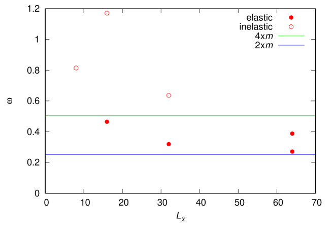
Figure 15: The two-particle state energy as a function of $L_{x}$. Here $m$ is the rest mass for one-particle state, and we set the value in eq.(67).

From the two-particle state energy $\omega$ in Table 3, one can determine the relative momentum $k$

$$\omega=2\sqrt{m^{2}+k^{2}},$$ (66)

where $m$ is the rest mass for one-particle state and here we set exact value for $L_{x}=64$,

$$m=0.1262302.$$ (67)

By using the value of $k$, the phase shift $\delta(k)$ is determined from Lüscher’s formula [65]

$$e^{2i\delta(k)}=e^{-ikL_{x}}.$$ (68)

See Fig. 16 for the phase shift as a function of $k/m$. The tensor network results in the elastic region $k/m<\sqrt{3}$ are consistent with the theoretical expectation $\delta(k)=\delta_{\rm Ising}=-\pi/2$ [66].

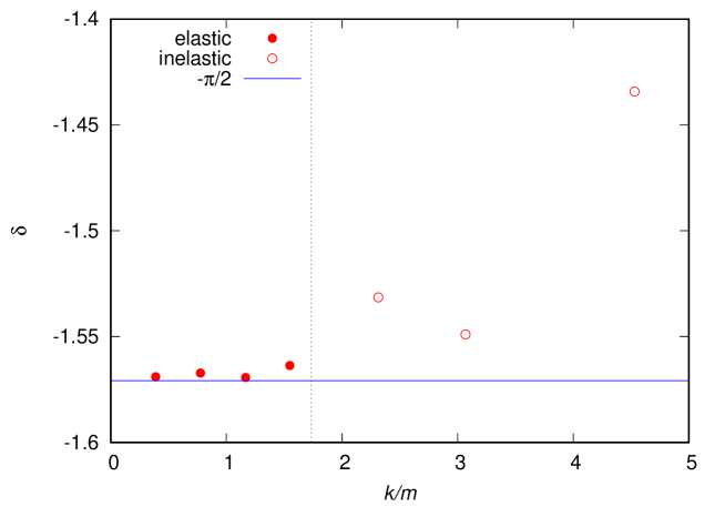
Figure 16: The phase shift as a function of $k/m$.

4 Summary

In the paper, we have proposed a spectroscopy scheme by combining with the transfer matrix formalism and the Lagrangian tensor network formulation. Using the new scheme, the energy spectrum can be simply obtained from the eigenvalues of the numerical transfer matrix that is formed by the coarse-grained tensors. The quantum number of the energy eigenstate is identified by the selection rule that requires the matrix element of some insertion operator sandwiched by the eigenstates. We have proposed the procedure to compute the matrix elements by using the impurity tensor network.

As a demonstration, we have studied the spectrum of $(1+1)$d Ising model whose exact spectrum is well known. We have confirmed that the energy spectrum and the quantum number are well reproduced up to 20 modes for $L_{x}=2^{6}$ in disordered phase $T=2.44>T_{\rm c}$. The accuracy of the lowest gap tends to be better around $T_{\rm c}$ in contrast to the free energy where the accuracy gets worse around the critical point. We have observed that the accuracy of the energy gaps tends to be worse for larger system size due to the truncation error in the coarse-graining step, and the systematic error becomes larger for higher excited states at the fixed system size. On the other hand, for larger bond dimension, the accuracy of the energy gap gets smoothly better. We also have computed the one-particle state wave function for the energy eigenstates and try to identify their momentum. To confirm the momentum identification using the wave function, we have proposed another procedure using the selection rule together with the proper matrix elements and then both results shown to be consistent. Relatively higher momentum states are properly identified and the dispersion relation is clearly observed. We also identify the two-particle states and obtain the scattering phase shift from their energy using Lüscher’s formula. The resulting phase shift is consistent with the theoretical expectation for Ising model.

In future, we plan to apply our new scheme to other quantum field theories.

Appendix A Transfer matrix and initial tensor for $(1+1)$d Ising model

Consider the Ising model on the square lattice $\Gamma$ in eq.(10) with the zero external magnetic field. The Hamiltonian of the model is given by

$$H[s]=-J\sum_{{\bm{r}}\in\Gamma}\sum_{\mu=1}^{2}s({\bm{r}}+\hat{\mu})s({\bm{r}})$$ (69)

where the spin variables take $s({\bm{r}})=\pm 1$ and the interaction energy parameter $J$ is set to unity in the following. The partition function for the model is given by

$$Z=\sum_{\{s\}}e^{-\beta H}$$ (70)

with the inverse of temperature $\beta=T^{-1}$. The periodic boundary condition is applied to the system.

The partition function can be written in terms of transfer matrix

$$Z = \operatorname{Tr}\left[\mathcal{T}^{L_{\tau}}\right]$$ (71)

where the transfer matrix ${\cal T}$ for the Ising model is given by

$$\mathcal{T}_{S^{\prime}S} = \left(\prod_{x=0}^{L_{x}-1}\exp\left[\beta s(t+1,x)s(t,x)\right]\right)$$ (72)

$$\times \left(\prod_{x=0}^{L_{x}-1}\exp\left[\frac{\beta}{2}s(t+1,x+1)s(t+1,x)+\frac{\beta}{2}s(t,x+1)s(t,x)\right]\right).$$

The spin configurations on the Euclidean time slice at $t+1$ and $t$ are denoted by

$$S^{\prime} = \{s(t+1 x) | x=0,1,2,\cdots,L_{x}-1\},$$ , (73)

$$S = \{s(t x) | x=0,1,2,\cdots,L_{x}-1\}.$$ , (74)

To derive an initial tensor for the Ising model, first we apply the EVD to the local Boltzmann factor,

$$e^{\beta s^{\prime}s}=\sum_{k=1}^{2}u_{s^{\prime}k}\sigma_{k}(u^{\dagger})_{ks}\,\,\,\mbox{ for }s^{\prime},s=\pm 1$$ (75)

with

$$u_{sk}=\frac{1}{\sqrt{2}}\begin{pmatrix}1&1\\ 1&-1\end{pmatrix},~{}~{}\sigma_{k}=\begin{pmatrix}2\cosh\beta&0\\ 0&2\sinh\beta\end{pmatrix}.$$ (76)

By using the $u$ and $\sigma$, we define the initial tensor $A$ (see eq.(36) for the scalar field case)

$$A_{abcd}=\sqrt{\sigma_{a}\sigma_{b}\sigma_{c}\sigma_{d}}\sum_{s=\pm 1}(u^{\dagger})_{as}(u^{\dagger})_{bs}u_{sc}u_{sd}$$ (77)

where the indices $a,b,c,d$ take $1$ or $2$. For a single spin field ${\mathcal{O}}_{q}=s$ with $q=-1$, the associated impurity tensor (see eq.(46) for the scalar field case) is given by

$$A_{abcd}^{\prime}=\sqrt{\sigma_{a}\sigma_{b}\sigma_{c}\sigma_{d}}\sum_{s=\pm 1}s(u^{\dagger})_{as}(u^{\dagger})_{bs}u_{sc}u_{sd}.$$ (78)

Appendix B Exact spectrum of transfer matrix for $(1+1)$d Ising model

As given in [64], for the inverse temperature $\beta$ and the spatial lattice size $L_{x}$, the exact eigenvalues of the transfer matrix for $(1+1)$d Ising model is given by

$$(2\sinh(2\beta))^{L_{x}/2}\exp\left[\frac{1}{2}\left(\pm\gamma_{0}\pm\gamma_{2}\pm\gamma_{4}\pm\cdots\pm\gamma_{2L_{x}-2}\right)\right]\hskip 14.22636pt -$$ for sector (79)

$$(2\sinh(2\beta))^{L_{x}/2}\exp\left[\frac{1}{2}\left(\pm\gamma_{1}\pm\gamma_{3}\pm\gamma_{5}\pm\cdots\pm\gamma_{2L_{x}-1}\right)\right]\hskip 14.22636pt +$$ for sector (80)

where the even number of $+$ combination are only selected for each sector, thus there are in total $2\times 2^{L_{x}-1}$ eigenvalues. Here $\gamma_{n}$ ($n=1,2,...,2L_{x}$ and $\gamma_{0}=\gamma_{2L_{x}}$) is obtained by solving equation

$$\cosh\gamma_{n} = \cosh(2\beta^{\ast})\cosh(2\beta)-\cos\left(\frac{n\pi}{L_{x}}\right)\sinh(2\beta^{\ast})\sinh(2\beta),$$ (81)

where $\beta^{\ast}$ is defined from $e^{-2\beta}=\tanh\beta^{\ast}.$

References

- [1] M. Wagner, S. Diehl, T. Kuske, and J. Weber. An introduction to lattice hadron spectroscopy for students without quantum field theoretical background. arXiv 1310.1760.
- [2] H. Wittig. QCD on the Lattice. Springer International Publishing, Cham, 2020.
- [3] R. L. Workman and Others. Review of Particle Physics. PTEP, 2022:083C01, 2022.
- [4] M. C. Bañuls and K. Cichy. Review on Novel Methods for Lattice Gauge Theories. Rept. Prog. Phys., 83(2):024401, 2020.
- [5] K. Okunishi, T. Nishino, and H. Ueda. Developments in the Tensor Network — from Statistical Mechanics to Quantum Entanglement. J. Phys. Soc. Jap., 91(6):062001, 2022.
- [6] D. Kadoh. Recent progress in the tensor renormalization group. PoS, LATTICE2021:633, 2022.
- [7] S. R. White. Density matrix formulation for quantum renormalization groups. Phys. Rev. Lett., 69:2863–2866, Nov 1992.
- [8] S. Östlund and S. Rommer. Thermodynamic limit of density matrix renormalization. Phys. Rev. Lett., 75:3537–3540, Nov 1995.
- [9] F. Verstraete and J. I. Cirac. Renormalization algorithms for quantum-many body systems in two and higher dimensions. arXiv 0407066.
- [10] Mari Carmen Bañuls, Krzysztof Cichy, J. Ignacio Cirac, K. Jansen, and S. Kühn. Density Induced Phase Transitions in the Schwinger Model: A Study with Matrix Product States. Phys. Rev. Lett., 118(7):071601, 2017.
- [11] M. C. Bañuls et al. Simulating Lattice Gauge Theories within Quantum Technologies. Eur. Phys. J. D, 74(8):165, 2020.
- [12] M. C. Bañuls, K. Cichy, Y.-J. Kao, C. J. D. Lin, Y.-P. Lin, and D. T. L. Tan. Phase structure of the ( 1+1 )-dimensional massive Thirring model from matrix product states. Phys. Rev. D, 100(9):094504, 2019.
- [13] M. Schneider. The Hubbard model on a honeycomb lattice with fermionic tensor networks. PhD thesis, Humboldt U., Berlin, 2022.
- [14] Y. Shimizu. Analysis of the -dimensional lattice model using the tensor renormalization group. Chin. J. Phys., 50:749, 2012.
- [15] Y. Shimizu. Tensor renormalization group approach to a lattice boson model. Mod. Phys. Lett. A, 27:1250035, 2012.
- [16] J. F. Yu, Z. Y. Xie, Y. Meurice, Y. Liu, A. Denbleyker, H. Zou, M. P. Qin, and J. Chen. Tensor Renormalization Group Study of Classical XY Model on the Square Lattice. Phys. Rev. E, 89(1):013308, 2014.
- [17] H. Zou, Y. Liu, C.-Y. Lai, J. Unmuth-Yockey, A. Bazavov, Z. Y. Xie, T. Xiang, S. Chandrasekharan, S. W. Tsai, and Y. Meurice. Progress towards quantum simulating the classical O(2) model. Phys. Rev. A, 90(6):063603, 2014.
- [18] Y. Shimizu and Y. Kuramashi. Grassmann tensor renormalization group approach to one-flavor lattice Schwinger model. Phys. Rev. D, 90(1):014508, 2014.
- [19] Y. Shimizu and Y. Kuramashi. Critical behavior of the lattice Schwinger model with a topological term at using the Grassmann tensor renormalization group. Phys. Rev. D, 90(7):074503, 2014.
- [20] S. Takeda and Y. Yoshimura. Grassmann tensor renormalization group for the one-flavor lattice Gross–Neveu model with finite chemical potential. PTEP, 2015(4):043B01, 2015.
- [21] L.-P. Yang, Y. Liu, H. Zou, Z. Y. Xie, and Y. Meurice. Fine structure of the entanglement entropy in the O(2) model. Phys. Rev. E, 93(1):012138, 2016.
- [22] H. Kawauchi and S. Takeda. Tensor renormalization group analysis of CP(N-1) model. Phys. Rev. D, 93(11):114503, 2016.
- [23] Y. Shimizu and Y. Kuramashi. Berezinskii-Kosterlitz-Thouless transition in lattice Schwinger model with one flavor of Wilson fermion. Phys. Rev. D, 97(3):034502, 2018.
- [24] D. Kadoh, Y. Kuramashi, Y. Nakamura, R. Sakai, S. Takeda, and Y. Yoshimura. Tensor network formulation for two-dimensional lattice = 1 Wess-Zumino model. JHEP, 03:141, 2018.
- [25] D. Kadoh, Y. Kuramashi, Y. Nakamura, R. Sakai, S. Takeda, and Y. Yoshimura. Tensor network analysis of critical coupling in two dimensional theory. JHEP, 05:184, 2019.
- [26] Y. Kuramashi and Y. Yoshimura. Three-dimensional finite temperature Z2 gauge theory with tensor network scheme. JHEP, 08:023, 2019.
- [27] Y. Kuramashi and Y. Yoshimura. Tensor renormalization group study of two-dimensional U(1) lattice gauge theory with a term. JHEP, 04:089, 2020.
- [28] A. Bazavov, S. Catterall, R. G. Jha, and J. Unmuth-Yockey. Tensor renormalization group study of the non-Abelian Higgs model in two dimensions. Phys. Rev. D, 99(11):114507, 2019.
- [29] S. Akiyama, Y. Kuramashi, T. Yamashita, and Y. Yoshimura. Phase transition of four-dimensional Ising model with higher-order tensor renormalization group. Phys. Rev. D, 100(5):054510, 2019.
- [30] S. Akiyama, D. Kadoh, Y. Kuramashi, T. Yamashita, and Y. Yoshimura. Tensor renormalization group approach to four-dimensional complex theory at finite density. JHEP, 09:177, 2020.
- [31] S. Akiyama, Y. Kuramashi, T. Yamashita, and Y. Yoshimura. Restoration of chiral symmetry in cold and dense Nambu–Jona-Lasinio model with tensor renormalization group. JHEP, 01:121, 2021.
- [32] S. Akiyama, Y. Kuramashi, and Y. Yoshimura. Phase transition of four-dimensional lattice 4 theory with tensor renormalization group. Phys. Rev. D, 104(3):034507, 2021.
- [33] S. Akiyama and Y. Kuramashi. Tensor renormalization group approach to (1+1)-dimensional Hubbard model. Phys. Rev. D, 104(1):014504, 2021.
- [34] S. Akiyama, Y. Kuramashi, and T. Yamashita. Metal–insulator transition in the (2+1)-dimensional Hubbard model with the tensor renormalization group. PTEP, 2022(2):023I01, 2022.
- [35] K. Nakayama, L. Funcke, K. Jansen, Y.-J. Kao, and S. Kühn. Phase structure of the CP(1) model in the presence of a topological -term. Phys. Rev. D, 105(5):054507, 2022.
- [36] S. Akiyama and Y. Kuramashi. Tensor renormalization group study of (3+1)-dimensional 2 gauge-Higgs model at finite density. JHEP, 05:102, 2022.
- [37] S. Akiyama and Y. Kuramashi. Critical endpoint of (3+1)-dimensional finite density 3 gauge-Higgs model with tensor renormalization group. JHEP, 10:077, 2023.
- [38] T. Kuwahara and A. Tsuchiya. Toward tensor renormalization group study of three-dimensional non-Abelian gauge theory. PTEP, 2022(9):093B02, 2022.
- [39] M. Hirasawa, A. Matsumoto, J. Nishimura, and A. Yosprakob. Tensor renormalization group and the volume independence in 2D U(N) and SU(N) gauge theories. JHEP, 12:011, 2021.
- [40] M. Fukuma, D. Kadoh, and N. Matsumoto. Tensor network approach to two-dimensional Yang–Mills theories. PTEP, 2021(12):123B03, 2021.
- [41] J. Bloch, R. G. Jha, R. Lohmayer, and M. Meister. Tensor renormalization group study of the three-dimensional O(2) model. Phys. Rev. D, 104(9):094517, 2021.
- [42] X. Luo and Y. Kuramashi. Tensor renormalization group approach to (1+1)-dimensional SU(2) principal chiral model at finite density. Phys. Rev. D, 107(9):094509, 2023.
- [43] J. Bloch and R. Lohmayer. Grassmann higher-order tensor renormalization group approach for two-dimensional strong-coupling QCD. Nucl. Phys. B, 986:116032, 2023.
- [44] R. G. Jha. Tensor renormalization of three-dimensional Potts model. arXiv 2201.01789.
- [45] M. C. Bañuls, K. Cichy, K. Jansen, and J. I. Cirac. The mass spectrum of the Schwinger model with Matrix Product States. JHEP, 11:158, 2013.
- [46] E. Itou, A. Matsumoto, and Y. Tanizaki. Calculating composite-particle spectra in Hamiltonian formalism and demonstration in 2-flavor QED1+1d. JHEP, 11:231, 2023.
- [47] C.-Y. Huang, S.-H. Chan, Y.-J. Kao, and P. Chen. Tensor network based finite-size scaling for two-dimensional ising model. Phys. Rev. B, 107:205123, May 2023.
- [48] A. Ueda and M. Oshikawa. Finite-size and finite bond dimension effects of tensor network renormalization. Phys. Rev. B, 108:024413, Jul 2023.
- [49] M. Levin and C. P. Nave. Tensor renormalization group approach to two-dimensional classical lattice models. Phys. Rev. Lett., 99:120601, Sep 2007.
- [50] Z. Y. Xie, J. Chen, M. P. Qin, J. W. Zhu, L. P. Yang, and T. Xiang. Coarse-graining renormalization by higher-order singular value decomposition. Phys. Rev. B, 86:045139, Jul 2012.
- [51] Z. Y. Xie, H. C. Jiang, Q. N. Chen, Z. Y. Weng, and T. Xiang. Second renormalization of tensor-network states. Phys. Rev. Lett., 103:160601, Oct 2009.
- [52] G. Evenbly and G. Vidal. Tensor network renormalization. Phys. Rev. Lett., 115(18):180405, 2015.
- [53] S. Yang, Z.-C. Gu, and X.-. Wen. Loop optimization for tensor network renormalization. Phys. Rev. Lett., 118(11):110504, 2017.
- [54] M. Hauru, C. Delcamp, and S. Mizera. Renormalization of tensor networks using graph independent local truncations. Phys. Rev. B, 97(4):045111, 2018.
- [55] S. Morita, R. Igarashi, H.-H. Zhao, and N. Kawashima. Tensor renormalization group with randomized singular value decomposition. Phys. Rev. E, 97(3):033310, 2018.
- [56] K. Harada. Entanglement branching operator. Phys. Rev. B, 97(4):045124, 2018.
- [57] Y. Nakamura, H. Oba, and S. Takeda. Tensor renormalization group algorithms with a projective truncation method. Phys. Rev. B, 99:155101, 2019.
- [58] D. Adachi, T. Okubo, and S. Todo. Anisotropic tensor renormalization group. Phys. Rev. B, 102:054432, Aug 2020.
- [59] D. Kadoh and K. Nakayama. Renormalization group on a triad network. arXiv 1912.02414.
- [60] D. Kadoh, H. Oba, and S. Takeda. Triad second renormalization group. JHEP, 04:121, 2022.
- [61] E. Arai, H. Ohki, S. Takeda, and M. Tomii. All-mode renormalization for tensor network with stochastic noise. Phys. Rev. D, 107(11):114515, 2023.
- [62] K. Nakayama. Randomized higher-order tensor renormalization group. arXiv 2307.14191.
- [63] K. Homma and N. Kawashima. Nuclear norm regularized loop optimization for tensor network. arXiv 2306.17479.
- [64] B. Kaufman. Crystal statistics. ii. partition function evaluated by spinor analysis. Phys. Rev., 76:1232–1243, Oct 1949.
- [65] M. Luscher and U. Wolff. How to Calculate the Elastic Scattering Matrix in Two-dimensional Quantum Field Theories by Numerical Simulation. Nucl. Phys. B, 339:222–252, 1990.
- [66] C. R. Gattringer and C. B. Lang. Resonance scattering phase shifts in a 2-d lattice model. Nucl. Phys. B, 391:463–482, 1993.
- [67] M. Luscher. Volume Dependence of the Energy Spectrum in Massive Quantum Field Theories. 1. Stable Particle States. Commun. Math. Phys., 104:177, 1986.
- [68] M. Luscher. Volume Dependence of the Energy Spectrum in Massive Quantum Field Theories. 2. Scattering States. Commun. Math. Phys., 105:153–188, 1986.
- [69] M. Lüscher. Two-particle states on a torus and their relation to the scattering matrix. Nucl. Phys. B, 354(2):531–578, 1991.
- [70] M. Gockeler, H. A. Kastrup, J. Westphalen, and F. Zimmermann. Scattering phases on finite lattices in the broken phase of the four-dimensional O(4) phi**4 theory. Nucl. Phys. B, 425:413–448, 1994.
- [71] K. Rummukainen and S. Gottlieb. Resonance scattering phase shifts on a non-rest-frame lattice. Nucl. Phys. B, 450(1):397–436, 1995.
- [72] T. Yamazaki et al. I = 2 pi pi scattering phase shift with two flavors of O(a) improved dynamical quarks. Phys. Rev. D, 70:074513, 2004.
- [73] S. Aoki et al. I=2 pion scattering length from two-pion wave functions. Phys. Rev. D, 71:094504, 2005.
- [74] I. Montvay and G. Münster. Quantum Fields on a Lattice. Cambridge Monographs on Mathematical Physics. Cambridge University Press, 1994.
- [75] S. Morita and N. Kawashima. Calculation of higher-order moments by higher-order tensor renormalization group. Comp. Phys. Comm., 236:65–71, 2019.