Exact Cluster Dynamics of Indirect Reciprocity in Complete Graphs

Abstract

Heider’s balance theory emphasizes cognitive consistency in assessing others, as is expressed by “The enemy of my enemy is my friend.” At the same time, the theory of indirect reciprocity provides us with a dynamical framework to study how to assess others based on their actions as well as how to act toward them based on the assessments. Well-known are the ‘leading eight’ from L1 to L8, the eight norms for assessment and action to foster cooperation in social dilemmas while resisting the invasion of mutant norms prescribing alternative actions. In this work, we begin by showing that balance is equivalent to stationarity of dynamics only for L4 and L6 (Stern Judging) among the leading eight. Stern Judging reflects an intuitive idea that good merits reward whereas evil warrants punishment. By analyzing the dynamics of Stern Judging in complete graphs, we prove that this norm almost always segregates the graph into two mutually hostile groups as the graph size grows. We then compare L4 with Stern Judging: The only difference of L4 is that a good player’s cooperative action toward a bad one is regarded as good. This subtle difference transforms large populations governed by L4 to a “paradise” where cooperation prevails and positive assessments abound. Our study thus helps us understand the relationship between individual norms and their emergent consequences at a population level, shedding light on the nuanced interplay between cognitive consistency and segregation dynamics.

I Introduction

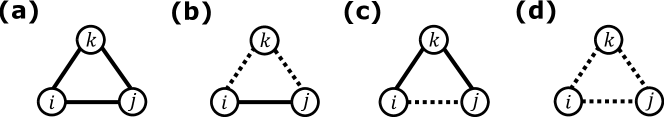
Figure 1: Configurations of three vertices, where solid and dashed lines mean good and bad relations, respectively. (a) Paradise in which everyone regards everyone as good ($+1$). (b) Another balanced configuration which divides the three vertices into two mutually hostile clusters, i.e., $\{i,j\}$ and $\{k\}$, so that the members of one cluster assess those in the other cluster as bad ($-1$). (c) An unbalanced configuration in which $i$ assesses $j$ as bad although $j$ is $i$’s friend’s friend (d) Another example of the lack of balance, in which $i$ assesses $j$ as bad although $j$ is $i$’s enemy’s enemy.

Heider’s balance theory is a minimal model of consistency in human relations Heider (1946). Because of its mathematical simplicity, the balance theory has opened up an interdisciplinary field between psychology and graph theory Harary (1953); Cartwright and Harary (1956). Between each given pair of individuals, the theory assumes a binary relation, which can be represented either by $+1$ if positive (e.g., they like each other) or by $-1$ if negative (e.g., they dislike each other). The basic unit of the balance theory is a triangle as shown in Fig. 1, where vertices and edges represent individuals and their relations, respectively. If the triangle contains an even number of negative edges, it is balanced because everyone can clearly distinguish friend and foe: In Fig. 1(a), everyone is positively related to each other. In Fig. 1(b), the relation between $i$ and $j$ is positive, which is consistent with the fact that they both have negative relations with $k$. Mathematically speaking, the direct edge between $i$ and $j$ is represented by $\sigma_{ij}=+1$, which is exactly identical to the product of $\sigma_{ik}=-1$ and $\sigma_{kj}=-1$, where $\sigma_{xy}=\sigma_{yx}$ for every possible pair of $x$ and $y$ in an undirected graph. The product $\sigma_{ik}\sigma_{kj}$ is called the sign of this path from $i$ to $j$ via $k$. In general, for any graph with positive and negative edges, we say that it is balanced if and only if all paths joining the same pair of vertices have the same sign. By contrast, in the other two cases of Fig. 1(c) and (d), one feels ‘tension’ because, e.g., one has a positive relation with his or her friend’s enemy so that two paths connecting the same pair of individuals have different signs.

Of particular importance is the structure theorem Harary (1953); Cartwright and Harary (1956), which states that a graph is balanced if and only if the graph is separated into two clusters in such a way that every edge inside a cluster is positive whereas any edge between the clusters is negative. Let us define the size of a cluster as the number of vertices inside it. In a balanced configuration, the size of one of the clusters can be zero, in which case, all the edges are positive, and such a configuration is called paradise Antal et al. (2005). The idea behind this structure theorem is that friends and foes are defined without ambiguity from an arbitrary individual’s perspective in a balanced configuration: Those with positive relations to the focal individual constitute one cluster, and those with negative relations constitute the other.

The balance theory is static, and one could naturally ask which dynamics leads to a balanced configuration. The first attempt was a discrete-time model, in which a randomly chosen edge is flipped to achieve more balance, either locally or globally Antal et al. (2005). One version of this discrete-time model corresponds to an Ising-spin system with the following Hamiltonian:

$$H=-\sum_{\left<ijk\right>}\sigma_{ij}\sigma_{jk}\sigma_{ki},$$ (1)

where the summation runs over all triangles of the underlying graph Malarz and Hołyst (2022); Wołoszyn and Malarz (2022); Malarz and Wołoszyn (2023). By making thermal contact with a heat bath at temperature $T$, this Hamiltonian system undergoes stochastic time evolution, which was expected to guide the system to a balanced configuration as $T\to 0$. However, it has turned out that such local dynamics also generates infinitely many stable yet unbalanced configurations Marvel et al. (2009). An alternative, continuous-time model with real-valued $\sigma_{ij}$’s has thus been studied to prove that a balanced configuration is almost always reached from a random initial configuration in finite time, if a large number of vertices are connected by a complete graph Kułakowski et al. (2005); Marvel et al. (2011).

In this work, we study dynamics of indirect reciprocity as another way to approach structural balance. An individual’s deed to another can be reciprocated indirectly from a third-party observer, and this mechanism is regarded as a powerful mechanism of establishing cooperation among individuals Alexander (1987); Nowak and Sigmund (2005). The mechanism of indirect reciprocity typically involves three persons: An actor, also called a donor, and a recipient of the donation from the donor, and an observer watching those two persons and updating his or her own assessment of the donor. The donor may either cooperate by choosing donation or defect by doing nothing to the recipient. Note that this dynamics has directionality because $\sigma_{ij}$ is not necessarily the same as $\sigma_{ji}$. An early issue of debate in indirect reciprocity was whether a first-order assessment rule, relying only on the donor’s action, is sufficient for stabilizing the paradise Nowak and Sigmund (1998); Leimar and Hammerstein (2001); Sugden (1986), and the answer, at least in theory, is that the observer should use information of the recipient as well, in such a way that refusing to cooperate to a bad recipient does not damage the donor’s image to the observer Ohtsuki and Iwasa (2004, 2006).

Among such good higher-order assessment rules, which are now called ‘leading eight’ and shown in Table 1, a particularly well-known example is what we will call L6 throughout this work (also known as ‘Stern Judging’ or ‘Kandori’) Kandori (1992); Pacheco et al. (2006); Santos et al. (2018). According to this simple and intuitive norm, a donor must donate only when he or she regards the recipient as good, and whether the donor’s cooperation looks good to an observer heavily relies on the recipient’s image to the observer. The assessment rule of L6 can thus be algebraically expressed as Oishi et al. (2021)

$$\sigma_{od}^{\prime}=\sigma_{or}\sigma_{dr},$$ (2)

where the prime means an updated value at the next time step, and the subscripts $d$, $r$, and $o$ mean the donor, recipient, and observer, respectively. For example, as represented by $\sigma_{or}$ on the right-hand side, the observer’s assessment of the donor at the next time step will indeed be affected by how the observer thinks about the recipient. The squared difference between the current and next values of $\sigma_{od}$ is

$$\left(\sigma_{od}-\sigma_{od}^{\prime}\right)^{2}=\left(\sigma_{od}-\sigma_{or}\sigma_{dr}\right)^{2}=2-2\sigma_{od}\sigma_{or}\sigma_{dr},$$ (3)

where we have used $(\pm 1)^{2}=1$. Therefore, we will find $\sigma_{od}^{\prime}=\sigma_{od}$ if and only if $\sigma_{od}\sigma_{or}\sigma_{dr}=1$, and this condition is certainly reminiscent of the Hamiltonian approach in Eq. (1), although we will later point out its important difference from Eq. (2). L6 has its own weaknesses: Once it deviates from the paradise, L6 fails to return in the presence of noisy and private assessment Hilbe et al. (2018); Lee et al. (2021, 2022); Mun and Baek (2023). It is rather known that L6 would divide a fully connected society into two mutually hostile clusters Oishi et al. (2013), consistently with the structure theorem of the balance theory. On the other hand, if the society uses L4, which is almost identical to L6, our numerical simulations show that it easily reaches the paradise. The only difference of L4 from L6 is that a good donor’s cooperation with a bad recipient does not damage the donor’s image from the observer’s viewpoint. The aim of this paper is to clarify the reason of such distinct outcomes, i.e., segregation and paradise.

We investigate the mechanism of segregation by using an exact analysis of the Markov dynamics in complete graphs. The analysis reveals that segregation of L6 is actually driven by entropy, whereas L4 introduces a bias toward the paradise, which becomes stronger as the system size increases. Considering such a small difference between the two norms, we propose that L4 can be the most promising remedy for segregation induced by the intuitive rules of L6.

Table 1: Prescriptions of the leading eight Ohtsuki and Iwasa (2004, 2006). We assume that an observer observes the interaction between a donor and a recipient and assesses the donor according to one of the following norms. Let $G$ and $B$ denote good and bad, respectively, and let $C$ and $D$ denote cooperation and defection, respectively. If $\alpha_{uXw}=G$($B$), the donor’s action $X\in\{C,D\}$ to the recipient, whose images to the observer are $u$ and $w$, respectively, is assessed as good (bad) by the observer. If $\beta_{uw}=C(D)$, the donor is prescribed to cooperate (defect) toward the recipient when their images to the donor are $u$ and $w$, respectively.

	$\alpha_{GCG}$	$\alpha_{GDG}$	$\alpha_{GCB}$	$\alpha_{GDB}$	$\alpha_{BCG}$	$\alpha_{BDG}$	$\alpha_{BCB}$	$\alpha_{BDB}$	$\beta_{GG}$	$\beta_{GB}$	$\beta_{BG}$	$\beta_{BB}$
L1	$G$	$B$	$G$	$G$	$G$	$B$	$G$	$B$	$C$	$D$	$C$	$C$
L2 (Consistent Standing)	$G$	$B$	$B$	$G$	$G$	$B$	$G$	$B$	$C$	$D$	$C$	$C$
L3 (Simple Standing)	$G$	$B$	$G$	$G$	$G$	$B$	$G$	$G$	$C$	$D$	$C$	$D$
L4	$G$	$B$	$G$	$G$	$G$	$B$	$B$	$G$	$C$	$D$	$C$	$D$
L5	$G$	$B$	$B$	$G$	$G$	$B$	$G$	$G$	$C$	$D$	$C$	$D$
L6 (Stern Judging)	$G$	$B$	$B$	$G$	$G$	$B$	$B$	$G$	$C$	$D$	$C$	$D$
L7 (Staying)	$G$	$B$	$G$	$G$	$G$	$B$	$B$	$B$	$C$	$D$	$C$	$D$
L8 (Judging)	$G$	$B$	$B$	$G$	$G$	$B$	$B$	$B$	$C$	$D$	$C$	$D$

II Model

Let us consider a directed graph with a set of vertices and a set of edges, which are denoted as $V$ and $E$, respectively. Every vertex has an agent, who has an opinion about each of the neighbors that are connected to the focal vertex by edges. For any random pair of two vertices, they are connected with probability $p$, and the connection structure is fixed during the dynamical evolution of edges. The structure is called a complete graph when $p=1$, which we mainly consider in this work. The cardinality of $V$ is the total number of vertices, or the population size, and we denote it as $N$. Opinions take discrete values, so $\sigma_{ij}=+1$ if $i$ regards $j$ as good, and $-1$ otherwise. Everyone shares an assessment rule and an action rule in common.

1. A donor $d$ is randomly chosen from $V$, and a recipient $r$ is chosen among $d$’s neighbors including $d$ itself.

2. The donor $d$ chooses whether to cooperate toward the recipient $r$ according to the action rule.

3. All neighbors of both $d$ and $r$ observe $d$’s action toward $r$. The set of observers includes $d$ and $r$ as well. Each and every observer $o$’s opinion about $d$, denoted as $\sigma_{od}$, is updated to $\sigma_{od}^{\prime}$ as prescribed by the given assessment rule with probability $1-\epsilon$, and to $-\sigma_{od}^{\prime}$ with probability $\epsilon\ll 1$, where $\epsilon$ is the probability of assessment error. We assume that actions are implemented without error.

III Results

III.1 Balance and stationarity

We begin by checking whether the balance condition is equivalent to stationarity for each of the leading eight. This analysis is necessary because it relates the balance condition, a static property, to stationarity, which is a dynamical consequence. The conclusion of this subsection is the following: Among the leading eight (Table 1), the balance condition can be identified with stationarity only for L6 and L4, the former of which has been analyzed in detail by one of us previously in the context of balance and group formation Oishi et al. (2013, 2021).

Regarding L6, we may rewrite its rule [Eq. (2)] as

$$\sigma_{od}^{\prime}=\sigma_{or}\sigma_{dr}=\sigma_{od}\sigma_{or}\sigma_{dr}\sigma_{od}=\Phi_{odr}\sigma_{od},$$ (4)

by using $\sigma_{od}^{2}=1$ and defining a local order parameter for triad balance,

$$\Phi_{odr}\equiv\sigma_{od}\sigma_{or}\sigma_{dr}.$$ (5)

The stationarity condition requires $\sigma_{od}^{\prime}=\Phi_{odr}\sigma_{od}=\sigma_{od}$ for an arbitrary triangle of $o$, $d$, and $r$. We thus conclude that stationarity is equivalent to the balance condition that $\Phi_{odr}=1$ Oishi et al. (2021).

As for L4, recall that its only difference from L6 is that a good donor’s cooperation toward a bad recipient is regarded as good (Table 1). However, the difference will never be observed in a balanced configuration if everyone follows the L4 rule, which prescribes a good donor to defect against a bad recipient. This indicates that balance implies stationarity in L4. The proof of the converse statement on L4, as well as discussions on the other norms of the leading eight, can be found in Appendix A.

III.2 Dynamics on complete graphs

Let us imagine all the possible $2^{N\times N}$ edge configurations on a complete graph, only one of which is the paradise. The question is whether the paradise will occupy $100\%$ of the stationary probability in the limit of $\epsilon\to 0$. One way to answer this question is to count the order of $\epsilon$ Murase and Baek (2020). That is, in the order of $\epsilon^{0}$, we consider only the transitions permitted by L6 or L4, according to which the dynamics ends up with one of balanced configurations. These sinks have no connections among themselves because balance means stationarity. Whether the probability flows will converge to the paradise is undecidable at this level of description. We then add links with probabilities of $O(\epsilon^{1})$ by considering transitions mediated by a single error. If the paradise appears as a global sink at this level of description, it will occupy $100\%$ in the limit of $\epsilon\to 0$. Or, if there is an outgoing flow of $O(\epsilon)$ from the paradise, we conclude that it cannot occupy the whole stationary probability. If it is still undecidable, we add links of $O(\epsilon^{2})$ and repeat the analysis. For our current purpose, the description of $O(\epsilon)$ is sufficient because a single error can change one balanced configuration to another as will be detailed below.

III.2.1 Path-reversal symmetry in L6

To investigate the cluster dynamics under L6, we begin by showing the following: At a balanced configuration with two clusters, a single error can move at most a vertex from a cluster to the other cluster. Let us start with a balanced configuration dividing $V$ into two partitions, i.e.,

$$P_{\text{balance}}=\{\{v_{1},\ldots,v_{n}\},\{v_{n+1},\ldots,v_{N}\}\},$$ (6)

where $1\leq n<N$. The paradise is represented by a trivial partition

$$P_{\text{paradise}}=\{V\},$$ (7)

which we regard as a special case of $P_{\text{balance}}$ with $n=N$ by a slight abuse of notation to allow a partition to be empty. Without loss of generality, we assume that $v_{n}$ has committed an assessment error, after which all time evolution strictly follows the common social norm L6. To be more specific, the focal individual $v_{n}$ commits an error either by assessing its friend as bad or by assessing its enemy as good, so $V$ can be divided into the following five partitions, some of which may be empty (Fig. 2):

Figure 2: Reduction to a five-vertex configuration under an assumption that $v_{n}$ has committed error in assessment. The former friends of $v_{n}$ are the members of $\pi_{1}$ and $\pi_{2}$, of which $v_{n}$ now dislikes the latter. The former enemies of $v_{n}$ are the members of $\pi_{3}$ and $\pi_{4}$, of which $v_{n}$ still dislikes the latter.

$$P_{\text{error}}=\{\underbrace{\{\ldots\}}_{\pi_{1}},\underbrace{\{\ldots\}}_{\pi_{2}},\{v_{n}\},\underbrace{\{\ldots\}}_{\pi_{3}},\underbrace{\{\ldots\}}_{\pi_{4}}\},$$ (8)

where $\pi_{1}\cup\pi_{2}=\{v_{1},\ldots,v_{n-1}\}$ and $\pi_{3}\cup\pi_{4}=\{v_{n+1},\ldots,v_{N}\}$. The members of $\pi_{1}$ and $\pi_{2}$ like $v_{n}$, but $v_{n}$ likes $\pi_{1}$ and dislikes $\pi_{2}$. The members of $\pi_{3}$ and $\pi_{4}$ dislike $v_{n}$, but $v_{n}$ likes $\pi_{3}$ and dislikes $\pi_{4}$. All members in each partition are the same in relation to those in another partition, so a partition can behave like a single vertex. The dynamics can also make the elements of $\pi_{1}$ go over to $\pi_{2}$ or vice versa, and the same applies to $\pi_{3}$ and $\pi_{4}$, but $v_{n}$ remains alone in its own partition because the dynamics has no more erroneous assessment. The important point is that the five-vertex picture in Eq. (8) will remain valid on the understanding that some of the partitions may be empty. When we exhaustively trace the time evolution of the corresponding five-vertex configurations by applying L6, the final outcome is always either the original balanced configuration $P_{\text{balance}}$ [Eq. (6)] or a new balanced one represented by

$$P^{\prime}_{\text{balance}}=\{\{v_{1},\ldots,v_{n-1}\},\{v_{n},\ldots,v_{N}\}\},$$ (9)

where $v_{n}$ now belongs to the latter partition. This completes the proof that an error can cause at most a single vertex to change its membership under L6.

One of our main findings is that every balanced configuration occupies equal stationary probability $B^{-1}$ in the limit of $\epsilon\to 0$, where $B=2^{N-1}$ is the number of balanced configurations (Appendix B). To prove this statement, we start from the rule of L6 [Eq. (2)], which we write here once again for the sake of convenience:

$$\sigma_{od}^{\prime}=\sigma_{or}\sigma_{dr}.$$

Let us assume that each player’s self-image has converged to $+1$ because $\sigma_{dd}^{\prime}=\sigma_{dr}^{2}=+1$. We may expect this convergence within $O(1)$ Monte Carlo steps Oishi et al. (2021). In addition, our analysis assumes that no error occurs in self-images. Our proof is based on the following property of L6: For any transition sequence of configurations permitted by the above rule of L6, if we choose an arbitrary vertex and flip all its edges, except the self-loop, we will get another valid sequence of configurations permitted by L6. It can be seen directly from the L6 rule itself: When the chosen vertex is a donor, flipping $\sigma_{od}^{\prime}$ and $\sigma_{dr}$ makes the equality hold, while leaving $\sigma_{dd}^{\prime}=+1$ unchanged. When the chosen vertex is a recipient, it assesses the donor with $\sigma_{rd}^{\prime}=\sigma_{dr}$, whose equality is unaffected by flipping both the sides. Finally, when the chosen vertex is an observer, flipping $\sigma_{od}^{\prime}$ and $\sigma_{or}$ again satisfies the above rule.

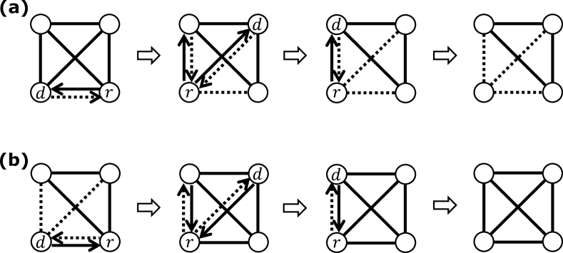
Figure 3: Path-reversal symmetry in L6: By flipping all the edges of a given vertex (at the lower left corner in this example), we get a transition path in the opposite direction with the same probability. (a) Error-induced transition from the paradise to a segregated balanced configuration with an isolated single vertex. The letters $d$ and $r$ show the donor and the recipient, respectively, at each time step. By each line without an arrow head between a pair of vertices, we mean that their relation is reciprocal, i.e., mutually good (solid) or mutually bad (dashed). The dashed right arrow in the leftmost diagram means that the individual chosen as $d$ has erroneously assessed the recipient $r$ as bad so that the donor will defect. (b) The opposite direction from a segregated configuration to the paradise. The solid right arrow in the leftmost diagram means that an isolated individual, playing the role of $d$, has erroneously assessed the recipient $r$ as good so that the donor will cooperate. Self-loops are all good by assumption and omitted from the diagrams for the sake of brevity.

In Fig. 3(a), we depict an error-induced sequence from the paradise to another balanced configuration where an individual conflicts with all the rest. Now, by choosing the vertex at the lower left corner and flipping all its edges, except its self-loop, we obtain Fig. 3(b). The point is that the sequence in Fig. 3(b) shows valid transitions back to the paradise, with exactly the same probability as its counterpart in Fig. 3(a). In general, for every sequence of transition from Eq. (6) to Eq. (9), the transformation applied to $v_{n}$ generates the corresponding sequence in the opposite direction with equal probability. In addition, as proved above, no more than a single vertex can change its cluster in this $O(\epsilon)$ description, which precludes the existence of any indirect transition paths connecting Eq. (6) and Eq. (9) via a third balanced configuration. Therefore, the total transition probability must be the same in either direction, satisfying Kolmogorov’s criterion. The resulting detailed-balance condition equalizes the stationary probabilities of Eq. (6) and Eq. (9). In other words, the paradise has the same stationary probability as any balanced configuration of two clusters with sizes $1$ and $N-1$, respectively, so we have

$$\rho_{\text{st}}\left[\{V\}\right]=\rho_{\text{st}}\left[\{\{v\},V-\{v\}\}\right],$$ (10)

where $\rho_{\text{st}}$ means stationary probability, and $v$ is an arbitrary element of $V$. By the same token, we also see that

$$\rho_{\text{st}}\left[\{\{v\},V-\{v\}\}\right]=\rho_{\text{st}}\left[\{\{v,v^{\prime}\},V-\{v,v^{\prime}\}\}\right],$$ (11)

where $v$ and $v^{\prime}$ are two arbitrary distinct elements of $V$. Extending this argument one by one, we can conclude that every balanced configuration has the same stationary probability, which equals $B^{-1}$ in the limit of $\epsilon\to 0$. The transitions among balanced configurations are schematically drawn in Fig. 4(a).

III.2.2 Probability flows under L4

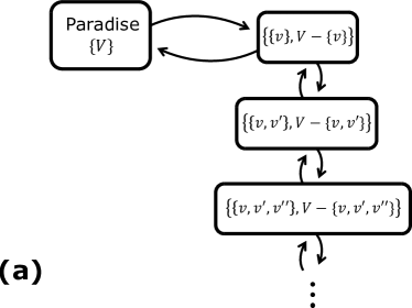
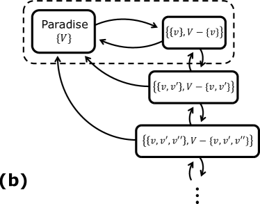
Figure 4: Schematic representation of transitions among balanced configurations under (a) L6 and (b) L4, where $v$, $v^{\prime}$, and $v^{\prime\prime}$ are arbitrary elements of $V$. Every arrow in the diagrams denotes a transition induced by a single assessment error, and the dashed box containing the transition between the paradise $\{V\}$ and $\{\{v\},V-\{v\}\}$ is detailed in Fig. 5.

According to our exhaustive enumeration, not only $P_{\text{balance}}$ and $P^{\prime}_{\text{balance}}$ [Eqs. (6) and (9)] but also $P_{\text{paradise}}=\{V\}$ becomes accessible from $P_{\text{error}}$ because L4 has $\alpha_{GCB}=G$ [Eq. (8)]. As a consequence, single-error transitions among balanced configurations under L4 are depicted as in Fig. 4(b). The important point is the existence of the one-way transition to the paradise, when both of the clusters have more than one vertex, as represented by $\{\{v,v^{\prime}\},V-\{v,v^{\prime}\}\}$ or $\{\{v,v^{\prime},v^{\prime\prime}\},V-\{v,v^{\prime},v^{\prime\prime}\}\}$ in Fig. 4. Such balanced configurations should have only negligible stationary probabilities because of the one-way transition. Still, the stationary probability of the paradise does not necessarily approach $100\%$ even with small $\epsilon$ because the system may go back and forth between the paradise and $\{\{v\},V-\{v\}\}$. For example, if $N=4$, our numerical estimate of $\rho_{\text{st}}\left[\left\{V\right\}\right]$ is only $61\%$ when $\epsilon=10^{-4}$, which is consistent with the order-counting argument Murase and Baek (2020).

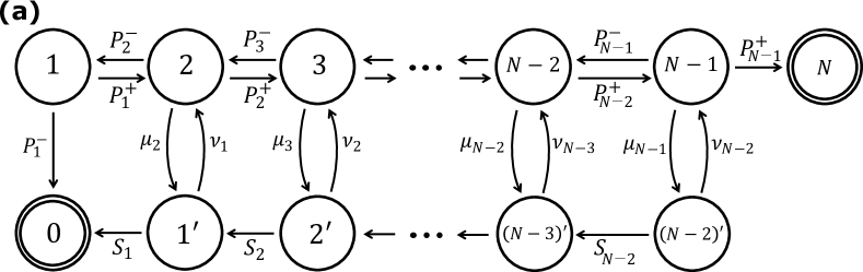
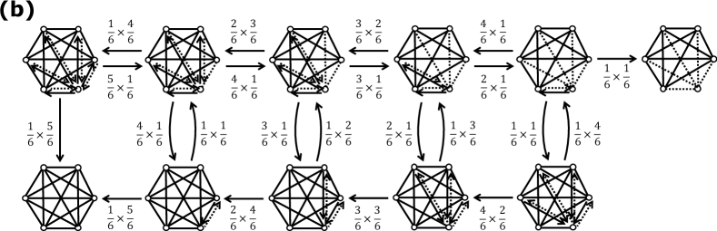
Figure 5: Zoomed-in views of the dashed box in Fig. 4, containing the transition between the paradise and $\{\{v\},V-\{v\}\}$. Self-loops are all omitted for the sake of brevity. (a) A schematic diagram where each node represents a set of configurations that are identical up to the permutation of vertices. The paradise and $\{\{v\},V-\{v\}\}$ are labeled with $0$ and $N$, respectively. The symbols attached to edges are transition probabilities. (b) An example of $N=6$ for the sake of concreteness.

However, the transition probability from $\{\{v\},V-\{v\}\}$ to the paradise becomes far greater than the opposite one as $N$ grows. Figure 5(a) provides a zoomed-in view for the dashed box of Fig. 4, where the nodes denoted by $0$ and $N$ correspond to the paradise and $\{\{v\},V-\{v\}\}$, respectively. Each node represents a set of edge configurations that are identical up to permutation of vertices. Figure 5(b) shows an example of $N=6$ for the sake of concreteness. The absorption probability into $\{\{v\},V-\{v\}\}$ from configuration $j$ is denoted by $q_{j}$, which means that $q_{0}=0$ and $q_{N}=1$ by definition. The symbols attached to the arrows in Fig. 5(a) are transition probabilities. For example, the configuration $1$ means that a vertex $v$ is disliked by all others whereas it still likes them. The next one denoted by $2$ means that $v$ now dislikes one of them. The transition from $1$ to $2$ occurs with probability $P_{1}^{+}=1/N\times(N-1)/N$ because $v$ must be the recipient with probability $1/N$ while anyone else can be chosen as the donor with probability $(N-1)/N$. It is straightforward to see that $P_{j}^{+}=(1/N)\times(N-j)/N$. The reverse transition from $2$ to $1$ happens with probability $P_{2}^{-}=(1/N)\times(N-2)/N$ because the one who $v$ dislikes ($1$ out of $N$) must donate someone who $v$ still likes ($N-2$ out of $N$). In general, we have $P_{j}^{-}=(N-j)/N\times(j-1)/N$. The exception is $P_{1}^{-}$, whose probability equals $P_{2}^{-}=(N-1)/N\times(1/N)$ because the transition happens when $v$ donates to anyone else. General expressions for the transition probabilities $\mu_{j}$, $\nu_{j}$, and $S_{j}$ are given in Appendix C.

If an assessment error occurs at the paradise, the starting point of the transition dynamics will be the configuration denoted by $1^{\prime}$ [see Fig. 5(b)]. The dynamics will end at $\{\{v\},V-\{v\}\}$ with probability $q_{1^{\prime}}$. Likewise, if an error occurs at $\{\{v\},V-\{v\}\}$ by assessing an enemy as good, the starting point will be the node denoted by $N-1$. The dynamics ends either at the paradise or at $\{\{v\},V-\{v\}\}$, so if we start from the one denoted by $N-1$, the probability of absorption into the paradise must be $1-q_{N-1}$. We wish to compare $q_{1^{\prime}}$ with $1-q_{N-1}$ to see the asymmetry in the probability flows: The random walk problem with two absorbing barriers as defined by Fig. 5 can be solved by recurrence formulas, which we provide in Appendix C. The solution shows that $(1-q_{N-1})/q_{1^{\prime}}$ is a rapidly increasing function of $N$, which outputs $15$, $82$, and $517$ for $N=4$, $5$, and $6$, respectively. It is instructive to consider the random walk only among the upper nodes without primes to get a lower bound of such asymmetry because the existence of the lower nodes, labeled with primes, should bias the net probability flow even more drastically toward the paradise. Although $q_{1^{\prime}}$ does not appear in this simplified problem, one can readily see that it is proportional to $q_{1}$ from Appendix C. The absorption probability of a one-dimensional random walker with position-dependent transition probabilities is a well-known problem in evolutionary game theory Nowak (2006): If we define

$$\gamma_{j}\equiv P_{j}^{-}/P_{j}^{+}=\left\{\begin{array}[]{ll}1&\text{for~{}}j=1\\ j-1&\text{for~{}}j>1,\end{array}\right.$$ (12)

it is straightforward to find that

$$q_{1} =\left[1+\sum_{i=1}^{N-1}\left(\prod_{j=1}^{i}\gamma_{j}\right)\right]^{-1}$$ (13a)

$$q_{k+1} =\left[1+\sum_{i=1}^{k}\left(\prod_{j=1}^{i}\gamma_{j}\right)\right]q_{1},$$ (13b)

where $k=1,\ldots,N-2$. One of its direct consequences is

$$\frac{1-q_{N-1}}{q_{1}}=\prod_{j=1}^{N-1}\gamma_{j}=(N-2)!,$$ (14)

which confirms that the net probability flow becomes more and more biased toward the paradise as $N$ increases. One could point out that we have not taken into account the existence of other paths from $\{\{v\},V-\{v\}\}$ to the paradise, e.g., through an error inside the larger cluster, but they can only contribute positively to the bias.

IV Discussion

Figure 6: Absolute difference of cluster sizes divided by $N$, obtained from $2\times 10^{2}$ Monte Carlo samples. Each sample starts from a random initial configuration and follows the common social norm with $\epsilon=0$ until arriving at a balanced configuration. Other simulation details are as described in Sec. II. We have defined $\eta\equiv\left|n-(N-n)\right|$, assuming that the clusters are of sizes $n$ and $N-n$, respectively. (a) Under L6, the behavior of $\eta/N$ is proportional to $N^{-1/2}$, which is fully consistent with a prediction from the binomial distribution. (b) Under L4, by contrast, $\eta/N$ tends to $1$ as $N$ grows, which implies the emergence of the paradise. The error bars are smaller than the symbol size.

Our first main finding is that every balanced configuration occupies equal stationary probability under the rule of L6. We have explicitly verified it for small values of $N$ by using the power method (not shown) and proved it for general $N$, as given above, in the limit of small $\epsilon$. Then, the segregation phenomenon induced by L6, which has been observed numerically Oishi et al. (2013), must be driven by entropy in the sense that the number of segregated balanced configurations greatly exceeds the unique possibility of the paradise as $N$ grows. The most probable case would be such that two clusters are of roughly equal sizes as in the binomial distribution. We can demonstrate it by using Monte Carlo simulations [Fig. 6(a)], according to which the size difference between two clusters, divided by $N$, decreases as $N^{-1/2}$. Note the different behavior of L4, according to which the paradise is easily accessible when $N\gtrsim O(10)$ [Fig. 6(b)]. This prediction is also partially supported by a recent analytic study Fujimoto and Ohtsuki (2022), showing that each individual is expected to receive good assessments from a half of the population, although it does not distinguish a clustered configuration from a randomly mixed one.

The uniform stationary probability among balanced configurations is contrasted with a result from the Hamiltonian in Eq. (1) because the paradise is locally stable in the Hamiltonian model Malarz and Hołyst (2022). Let us make sense of this difference: To define the Hamiltonian, every pair of vertices must be in a reciprocal relation, i.e., either mutually good or mutually bad, but it is approximately true in our setting as well because the convergence of $\sigma_{ij}\sigma_{ji}\to O(1)$ is a relatively fast process Oishi et al. (2021). We have to look at the zero-temperature Hamiltonian dynamics, derived from Eq. (1) as

$$\sigma_{ij}^{\prime}=\operatorname{sgn}\left(\sum_{k}\sigma_{ik}\sigma_{kj}\right),$$ (15)

where the summation runs over the common neighbors of $i$ and $j$ except themselves. Referring to those common neighbors is an important ingredient to ensure the local stability of the paradise because the peer pressure can correct an assessment error. In a sense, the Hamiltonian setting introduces surface tension in such a way that the Ising model is contrasted with the voter model Dornic et al. (2001). The difference of Eq. (15) from the L6 rule [Eq. (2)] is evident in a large complete graph, but it vanishes if the underlying structure allows every pair of vertices to have only one common neighbor. The same applies even to the case of two common neighbors, if we interpret $\operatorname{sgn}(0)$ as $\pm 1$ with equal probabilities.

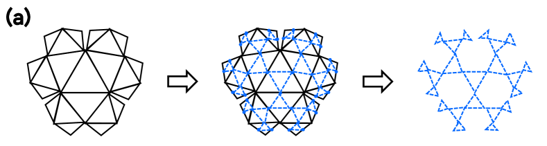
Figure 7: Line graphs obtained by transforming edges to vertices. (a) The line graph of the tree of triangles (solid) is the Husimi tree (dashed). (b) The line graph of the triangular lattice (solid) is the kagome lattice (dashed).

From the lack of directional preference in the transition among balanced configurations, we believe that the system governed by L6 with assessment error would be in a disordered phase until reaching a balanced configuration. One possible mechanism to hinder a balanced configuration could be quenched random removal of edges, which corresponds to the case of $p<1$ in our model (see Sec. II). When $p>O\left(N^{-1/2}\right)$ and $1-p>O\left(N^{-1}\right)$, the time to reach an absorbing state increases exponentially as $N$ grows Oishi et al. (2021), and this may also be a characteristic of a disordered phase. To support this idea, let us consider a sparse structure as depicted on the left in Fig. 7(a). Each edge is shared by two triangles, so we expect that it can be studied by using the Hamiltonian approach as an approximation. Considering that our $\sigma_{ij}$’s are defined on edges, whereas spin variables are usually defined on vertices, we take the line graph of the original structure, which turns out to be the Husimi tree. The three-spin interaction Hamiltonian model on the Husimi tree is exactly solved Monroe (1992); Ananikian and Dallakian (1997), and the solution tells us that it is in a disordered phase. We have summarized the solution in Appendix D for the sake of completeness. Another sparse structure that can be considered is the triangular lattice: In a Monte Carlo study, the Hamiltonian model on the triangular lattice has been reported to be disordered Malarz and Wołoszyn (2020). Its line graph is the kagome lattice [Fig. 7(b)], on which the exact solution of the three-spin Hamiltonian model again confirms that it is disordered Wu and Wu (1989); Barry and Muttalib (2019). All these observations indicate that a sparse structure would result in a disordered phase.

V Summary

In summary, we have analyzed cluster dynamics governed by L6 and L4, which becomes exact in the small-$\epsilon$ limit. We have explained why we focus on L6 and L4 among the leading eight by showing the equivalence between balance and stationarity. The dynamics of L6 has been studied by one of us Oishi et al. (2013, 2021), and the present work concludes that the segregation induced by L6 is a purely entropy-driven phenomenon.

This work has thus demonstrated the possibility of exact knowledge on cluster dynamics in this interdisciplinary field of social psychology, graph theory, and evolutionary game theory. It is worth pointing out that L6 is a remarkably simple and intuitive norm as indicated by its nickname ‘Stern Judging’: It assesses cooperation (defection) toward a good person as good (bad), and cooperation (defection) toward a bad person as bad (good). It thus prescribes cooperation toward a good person and defection toward a bad person. Despite all its good properties, L6 divides a fully connected society into two mutually hostile clusters which are of roughly equal sizes. The segregation might seem to be an ordered configuration compared to a random one, but the dominant factor behind it turns out to be entropy, and who belongs to which side is only a matter of chance. We propose L4 as a remedy for those problems: This norm leads a sufficiently large society of $N\gtrsim O(10)$ to the paradise just by changing the assessment of a good person’s cooperation toward a bad person. The change is so small that L4 still prescribes a good person to defect against the bad just as L6 does, and the defection would also be assessed as good. Furthermore, because of the clear bias toward the paradise, the system would not suffer long from disorder.

From a broader perspective, the precise understanding of segregation on fully connected graphs may give us theoretical insights into the recent trend of increasing political polarization in our hyper-connected society, as well as how to mitigate the trend with a minimal change in our judging behavior. Considering that the basic dynamics of a social norm would be preserved in more realistic acquaintance network structure Kuroda et al. (2023), we expect that our findings should also be relevant to real social phenomena.

Appendix A Balance and stationarity

A.1 L6 and L4

We may rewrite Eq. (2) as

$$\sigma_{od}^{\prime}=\sigma_{or}\sigma_{dr}=\sigma_{od}\sigma_{or}\sigma_{dr}\sigma_{od}=\Phi_{odr}\sigma_{od},$$ (16)

by using $\sigma_{od}^{2}=1$ and defining a local order parameter for triad balance,

$$\Phi_{odr}\equiv\sigma_{od}\sigma_{or}\sigma_{dr}.$$ (17)

The stationarity condition requires $\sigma_{od}^{\prime}=\Phi_{odr}\sigma_{od}=\sigma_{od}$ for an arbitrary triangle of $o$, $d$, and $r$. We thus conclude that stationarity is equivalent to the balance condition that $\Phi_{odr}=1$ Oishi et al. (2021).

The same statement holds true for L4. The assessment rule of L4 can be written as follows Lee et al. (2022):

$$\sigma_{od}^{\prime}=\frac{1}{4}\left(-\sigma_{or}+3\sigma_{dr}\sigma_{or}+\sigma_{dr}+\sigma_{dr}\sigma_{od}-\sigma_{or}\sigma_{od}+1+\sigma_{od}-\sigma_{dr}\sigma_{or}\sigma_{od}\right).$$ (18)

If the balance condition is met, we have $\Phi_{odr}=\sigma_{od}\sigma_{or}\sigma_{dr}=1$. It automatically means that

$$\sigma_{od} =\sigma_{or}\sigma_{dr}$$ (19a)

$$\sigma_{or} =\sigma_{od}\sigma_{dr}$$ (19b)

$$\sigma_{dr} =\sigma_{od}\sigma_{or}$$ (19c)

because $\sigma_{od}^{2}=\sigma_{or}^{2}=\sigma_{dr}^{2}=1$. Plugging these relations into Eq. (18), we obtain $\sigma_{od}^{\prime}=\sigma_{od}$ for an arbitrary $od$-pair, which means stationarity. Now, we have to check if the converse is true. The stationarity condition requires $\sigma_{od}^{\prime}=\sigma_{od}$, which leads to

$$\sigma_{od}=\frac{1}{4}\left(-\sigma_{or}+3\sigma_{dr}\sigma_{or}+\sigma_{dr}+\sigma_{dr}\sigma_{od}-\sigma_{or}\sigma_{od}+1+\sigma_{od}-\sigma_{dr}\sigma_{or}\sigma_{od}\right).$$ (20)

If we enumerate the eight possible cases of $(\sigma_{or},\sigma_{dr},\sigma_{od})=(\pm 1,\pm 1,\pm 1)$, Eq. (20) is satisfied for $(+1,+1,+1)$, $(-1,-1,+1)$, $(-1,+1,-1)$, $(+1,-1,-1)$, and $(-1,+1,+1)$, among which only the last one is unbalanced. To eliminate the last possibility, we note that stationarity is actually a stronger condition than Eq. (20): For a given configuration to be stationary, it must be left invariant even if we sample the three players in different order, so that $(\sigma_{or},\sigma_{dr},\sigma_{od})=(+1,-1,+1)$ and $(+1,+1,-1)$ must also satisfy Eq. (20), while neither of them is in the list. We thus exclude $(-1,+1,+1)$ from consideration and conclude that the balance condition is equivalent to stationarity in L4.

A.2 L3, L5, L7, and L8

By contrast, the balance condition is not equivalent to stationarity in L3 and L5. The assessment rule of L3 can be expressed as follows:

$$\sigma_{od}^{\prime}=\frac{1}{2}\left(1+\sigma_{dr}-\sigma_{or}+\sigma_{or}\sigma_{dr}\right).$$ (21)

Suppose that the balance condition $\Phi_{odr}=\sigma_{od}\sigma_{or}\sigma_{dr}=1$ is met. By using Eq. (19), we may rewrite Eq. (21) as

$$\sigma_{od}^{\prime}=\frac{1}{2}\big{[}1+\sigma_{od}(1+\sigma_{or}-\sigma_{dr})\big{]}.$$ (22)

If $(\sigma_{or},\sigma_{dr},\sigma_{od})=(-1,+1,-1)$, we see that stationarity is violated because $\sigma_{od}^{\prime}\neq\sigma_{od}$.

Likewise, the assessment rule of L5 can be represented as follows:

$$\sigma_{od}^{\prime}=\frac{1}{4}\left(-\sigma_{or}+3\sigma_{dr}\sigma_{or}+\sigma_{od}\sigma_{or}+1-\sigma_{od}+\sigma_{dr}\sigma_{od}\sigma_{or}+\sigma_{dr}-\sigma_{dr}\sigma_{od}\right)$$ (23)

Under the balance condition, together with Eq. (19), we obtain

$$\sigma_{od}^{\prime} = \frac{1}{4}[-\sigma_{or}+3\sigma_{dr}\sigma_{or}+\sigma_{od}\sigma_{or}+1-\sigma_{od}+1+\sigma_{dr}-\sigma_{dr}\sigma_{od}]$$ (24)

$$= \frac{1}{4}[-2\sigma_{or}+2\sigma_{od}+2\sigma_{dr}+2]=\frac{1}{2}[1+\sigma_{od}-\sigma_{or}+\sigma_{dr}]$$ (25)

Again, stationarity is violated if $(\sigma_{or},\sigma_{dr},\sigma_{od})=(-1,+1,-1)$. The balance condition is not equivalent to stationarity.

For L7 and L8, it is straightforward to prove inequivalence between stationarity and the balance condition. The reason is that both assign bad reputation when a bad donor defects against a bad recipient. A triad of $(\sigma_{or},\sigma_{dr},\sigma_{od})=(-1,-1,-1)$ is thus an absorbing configuration, although it is not balanced.

A.3 L1 and L2

For L1 and L2, a donor’s action to a recipient cannot simply be identified with $\sigma_{dr}$ from the beginning because a bad donor should cooperate to a bad recipient, i.e., $\beta_{BB}=C$ according to Table 1. For L1, a donor’s action can be coded as

$$\beta_{d}(\sigma_{dd},\sigma_{dr})=\frac{1}{2}\left[1+\sigma_{dd}(\sigma_{dr}-1)+\sigma_{dr}\right],$$ (26)

and an observer’s assessment rule is given as

$$\sigma_{od}^{\prime}=\frac{1}{4}\left[1+\sigma_{od}+3\beta_{d}-\sigma_{od}\beta_{d}+(1+\sigma_{od})(\beta_{d}-1)\sigma_{or}\right].$$ (27)

When $o=d$, we obtain $\sigma_{dd}^{\prime}=+1$ regardless of $\sigma_{dd}$ and $\sigma_{dr}$, so each donor’s self-evaluation quickly converges to $+1$. If $\sigma_{dd}=+1$ is plugged into Eq. (26), we can identify $\beta_{d}$ with $\sigma_{dr}$ as in the previous cases. Similarly, the assessment rule of L2 is

$$\sigma_{od}^{\prime}=\frac{1}{2}\beta_{d}\left[1+\sigma_{od}(\sigma_{or}-1)+\sigma_{or}\right],$$ (28)

where $\beta_{d}$ is given by Eq. (26). By setting $o=d$, we once again see the convergence toward $\sigma_{dd}^{\prime}=+1$ regardless of $\sigma_{dd}$ and $\sigma_{dr}$, which allows us to identify $\beta_{d}$ with $\sigma_{dr}$.

Therefore, for both L1 and L2, as soon as a donor’s action is fully prescribed from $\sigma_{dr}$, we can apply the same argument as above to prove the inequivalence between stationarity and the balance condition: A bad donor’s defection against a bad recipient is judged as bad by these norms, and this shows why $(\sigma_{or},\sigma_{dr},\sigma_{od})=(-1,-1,-1)$ is an unbalanced absorbing configuration.

Appendix B Number of balanced states

Assume that we have a set of vertices $V=\{v_{1},\ldots,v_{N}\}$. Thanks to the structure theorem, we just have to find the number of ways to divide those $N$ elements into two clusters. If none of the clusters is empty, we can prove that the answer is

$$W_{N}=2^{N-1}-1$$ (29)

by using mathematical induction. First, if $N=1$, we have no way to divide it into two nonempty clusters, which means that $W_{1}=0$. Second, let us assume that

$$W_{k}=2^{k-1}-1$$ (30)

for some positive integer $k$. When a new vertex $v_{k+1}$ has appeared, we have two possibilities to divide the $k+1$ elements into two clusters. One is to add $v_{k+1}$ to one of the existing clusters. The other is to make a single-element cluster of $v_{k+1}$ and merge the existing clusters into one. In other words, we have

$$W_{k+1}=2W_{k}+1.$$ (31)

Plugging Eq. (30) here, we find that

$$W_{k+1}=2\left(2^{k-1}-1\right)+1=2^{k}-1,$$ (32)

which proves Eq. (29) for general $N$. Note that $W_{N}$ does not include the paradise. If we take it into account, the number of balanced states is $B=2^{N-1}$ as mentioned in the main text.

Appendix C Recurrence formulas for L4

The absorption probabilities can be written as follows:

$$q_{j} =P_{j}^{-}q_{j-1}+P_{j}^{+}q_{j+1}+\mu_{j}q_{(j-1)^{\prime}}+\left(1-P_{j}^{-}-P_{j}^{+}-\mu_{j}\right)q_{j}$$ (33a)

$$q_{k^{\prime}} =S_{k}q_{(k-1)^{\prime}}+\nu_{k}q_{k+1}+\left(1-S_{k}-\nu_{k}\right)q_{k^{\prime}},$$ (33b)

where $j=1,\ldots,N-1$ and $k=1,\ldots,N-2$. By definition, we have $q_{0}\equiv 0$ and $q_{N}=1$. It is also convenient to define $q_{0^{\prime}}\equiv 0$ and $\mu_{1}\equiv 0$. We may rewrite the above formulas as

$$0 =P_{j}^{-}\left(q_{j-1}-q_{j}\right)+P_{j}^{+}\left(q_{j+1}-q_{j}\right)+\mu_{j}\left(q_{(j-1)^{\prime}}-q_{j}\right)$$ (34a)

$$q_{k+1} =\Gamma_{k}\left(q_{k^{\prime}}-q_{(k-1)^{\prime}}\right)+q_{k^{\prime}},$$ (34b)

where $\Gamma_{k}\equiv S_{k}/\nu_{k}$. Let us define $R_{k}\equiv q_{k^{\prime}}-q_{(k-1)^{\prime}}$. Plugging Eq. (34b) into Eq. (34a) and rearranging the terms, we obtain

$$P_{j}^{-}\Gamma_{j-2}R_{j-2}-\left[P_{j}^{-}(\Gamma_{j-1}+1)+P_{j}^{+}\Gamma_{j-1}+\mu_{j}\Gamma_{j-1}\right]R_{j-1}\\ +P_{j}^{+}(\Gamma_{j}+1)R_{j}=0.$$ (35)

The transition probabilities between unprimed nodes are given as follows:

$$P_{j}^{+} =\left(\frac{N-j}{N}\right)\left(\frac{1}{N}\right)$$ (36a)

$$P_{j}^{-} =\left\{\begin{array}[]{ll}\left(\frac{N-1}{N}\right)\left(\frac{1}{N}\right)&\text{for~{}}j=1\\ \left(\frac{j-1}{N}\right)\left(\frac{N-j}{N}\right)&\text{for~{}}j>1,\end{array}\right.$$ (36d)

as explained in the main text. Recall that we are denoting by $v$ the individual who has made an error. The transition probability $\mu_{j}$ corresponds to the case of choosing $v$ as the donor ($1$ out of $N$) and someone else who $v$ likes as the recipient ($N-j$ out of $N$). Its counterpart $\nu_{j}$ is the probability of choosing $v$ as the donor ($1$ out of $N$) and someone else who $v$ dislikes as the recipient ($j$ out of $N$). Finally, $S_{j}$ is the probability of choosing someone who $v$ dislikes as the donor ($j$ out of $N$) and someone else who $v$ likes (it can be $v$ itself) as the recipient ($N-j$ out of $N$). Therefore, their general expressions are

$$\mu_{j} =\left(\frac{N-j}{N}\right)\left(\frac{1}{N}\right)$$ (37a)

$$\nu_{j} =\left(\frac{1}{N}\right)\left(\frac{j}{N}\right)$$ (37b)

$$S_{j} =\left(\frac{j}{N}\right)\left(\frac{N-j}{N}\right),$$ (37c)

which results in $\Gamma_{j}=S_{j}/\nu_{j}=N-j$.

At $j=1$, Eq. (35) reduces to

$$P_{1}^{-}\left(-q_{1}\right)+P_{1}^{+}\left(\Gamma_{1}q_{1^{\prime}}+q_{1^{\prime}}-q_{1}\right)=0,$$ (38)

from which we obtain

$$R_{1}=q_{1^{\prime}}=\frac{P_{1}^{+}+P_{1}^{-}}{P_{1}^{+}\left(\Gamma_{1}+1\right)}q_{1}=\frac{2}{N}q_{1}.$$ (39)

At $j=2$, Eq. (35) takes the following form:

$$P_{2}^{-}\left[q_{1}-\left(\Gamma_{1}+1\right)R_{1}\right]+P_{2}^{+}\left[\left(\Gamma_{2}+1\right)R_{2}-\Gamma_{1}R_{1}\right]-\mu_{2}\Gamma_{1}R_{1}=0,$$ (40)

from which we find

$$R_{2}=\frac{5N-4}{N(N-1)}q_{1}.$$ (41)

From $j=3$ to $N-2$, we can find every $R_{j}$ from the following recurrence formula:

$$R_{j}=\frac{j-j^{2}+N+jN}{N-j+1}R_{j-1}-\frac{(j-1)(N-j+2)}{N-j+1}R_{j-2}.$$ (42)

Although we have $R_{k}$’s with $k=1,\ldots,N-2$, the overall factor of $q_{1}$ remains unknown, and it has to be determined from Eq. (35) at $j=N-1$:

$$P_{N-1}^{-}\left[\Gamma_{N-3}R_{N-3}-\left(1+\Gamma_{N-2}\right)R_{N-2}\right]$$ (43)

$$+ P_{N-1}^{+}\left[\left(1-q_{(N-2)^{\prime}}\right)-\Gamma_{N-2}R_{N-2}\right]-\mu_{N-1}\Gamma_{N-2}R_{N-2}=0,$$

where we have used $q_{N}=1$. By using the following identity,

$$q_{(N-2)^{\prime}}=\left(q_{(N-2)^{\prime}}-q_{(N-3)^{\prime}}\right)+\left(q_{(N-3)^{\prime}}-q_{(N-4)^{\prime}}\right)+\ldots+\left(q_{2^{\prime}}-q_{1^{\prime}}\right)+\left(q_{1^{\prime}}-q_{0^{\prime}}\right)=\sum_{k=1}^{N-2}R_{k},$$

we can write Eq. (43) in terms of $R_{j}$ only:

$$-(3N-6)R_{N-3}+(3N-2)R_{N-2}+\sum_{k=1}^{N-2}R_{k}=1,$$ (44)

from which we determine the value of $q_{1}$.

Appendix D Ising model on the Husimi tree

Let us consider a system of Ising spins with the following Hamiltonian, defined on the Husimi tree:

$$H=-J_{3}\sum_{\langle i,j,k\rangle}\sigma_{i}\sigma_{j}\sigma_{k}-J_{2}\sum_{\langle i,j\rangle}\sigma_{i}\sigma_{j}-h\sum_{i}\sigma_{i},$$ (45)

where $\langle i,j,k\rangle$ denotes a triangle of $i$,$j$, and $k$, and $\langle i.j\rangle$ means the nearest neighbors. Let us denote the spin at the center by $\sigma_{0}$, and define the following function:

$$\begin{split}g_{n}(\sigma_{0})&=\sum_{\{\sigma_{1}\}}\exp\Bigg{[}\tilde{\beta}\Bigg{(}J_{3}\sum_{\Delta}\sigma_{0}\sigma_{1}^{(1)}\sigma_{1}^{(2)}+J_{2}\left(\sigma_{0}\sigma_{1}+\sigma_{0}\sigma_{2}+\sigma_{1}\sigma_{2}\right)+h\sum_{j=1,2}\sigma_{1}^{(j)}\Bigg{)}\Bigg{]}\\ &\times[g_{n-1}(\sigma_{1}^{(1)})]^{\gamma-1}[g_{n-1}(\sigma_{1}^{(2)})]^{\gamma-1},\end{split}$$ (46)

where $\tilde{\beta}\equiv 1/(k_{B}T)$, and $\gamma$ is the number of triangles at each vertex, which is two as depicted in Fig. 7(a). By using $g_{n}(\sigma_{0})$, we can write the partition function as follows:

$$Z=\sum_{\sigma_{0}}\exp(\tilde{\beta}h\sigma_{0})[g_{n}(\sigma_{0})]^{\gamma}$$ (47)

Now, by defining $a\equiv e^{2\tilde{\beta}h}$, $b\equiv e^{2\tilde{\beta}J_{2}}$, and $c\equiv e^{2\tilde{\beta}J_{3}}$, we obtain the following map in terms of $z_{n}\equiv g_{n}(1)/g_{n}(-1)$ Monroe (1992):

$$z_{n}=y(z_{n-1}),\ y(z)=\frac{a^{2}b^{2}cz^{2(\gamma-1)}+2az^{\gamma-1}+c}{a^{2}z^{2(\gamma-1)}+2acz^{\gamma-1}+b^{2}}$$ (48)

The pure three-spin interaction Hamiltonian corresponds to $a=b=1$, in which case we have

$$y(z)=\frac{cz^{2}+2z+c}{z^{2}+2cz+1}$$ (49)

by setting $\gamma=2$. By solving $z=y(z)$, we obtain three fixed points, i.e., $z=-1$, $z=1$, and $z=-c$. However, $z=1$ is the only solution because $z$ cannot be negative. In addition, by drawing the map, we can see that $z=1$ is a stable fixed point. The local magnetization is expressed as Monroe (1992)

$$\langle\sigma_{0}\rangle=\frac{az_{n}^{\gamma}-1}{az_{n}^{\gamma}+1},$$ (50)

which is zero at $a=z=1$. However, the zero magnetization does not necessarily mean a disordered phase. To check the possibility of a phase transition, we will calculate the free energy. If it does not have a singularity at any finite temperature $T$, the system will always be in a disordered phase as in the high-temperature region. Let us rewrite the map by including both $a$ and $c$ as free parameters, while fixing $b=1$ and $\gamma=2$:

$$y(z)=\frac{a^{2}cz^{2}+2az+c}{a^{2}z^{2}+2acz+1}$$ (51)

By rearranging the terms of $z=y(z)$, we obtain the following quadratic equation of $a$:

$$(z^{3}-z^{2}c)a^{2}+2(z^{2}c-z)a+z-c=0,$$ (52)

which is solved by

$$a=\frac{1-cz\pm\sqrt{1-c^{2}-z^{2}+c^{2}z^{2}}}{z(z-c)}.$$ (53)

Noting that $a\geq 1$, $c\geq 1$, and $z>0$ by definition, the correct solution is given as follows:

$$a(c,z)=\frac{1-cz-\sqrt{1-c^{2}-z^{2}+c^{2}z^{2}}}{z(z-c)},$$ (54)

where $1\leq z<c$. This is a monotonically increasing function of $z$, and this property will be used later. The free-energy density can be written as follows Baxter (2007):

$$\tilde{\beta}f=-\frac{2}{3}\tilde{J_{3}}-\tilde{h}-\int^{\tilde{h}}_{\infty}[M(\tilde{h}^{\prime})-1]\ d\tilde{h}^{\prime},$$ (55)

where $\tilde{J_{3}}\equiv\tilde{\beta}J_{3}$ and $\tilde{h}\equiv\tilde{\beta}h$. The magnetic order parameter is denoted by $M=-\partial f/\partial h$, which we may identify with $\langle\sigma_{0}\rangle$ because of the translational symmetry of the lattice. The first two terms on the right-hand side is a constant of integration, which corresponds to the value in an ordered phase with $M=1$. We obtain $\tilde{h}$ from Eq. (54) and differentiate it with respect to $z$ for $\partial\tilde{h}/\partial z$. We thus calculate the free-energy density as

$$\tilde{\beta}f=-\frac{2}{3}\tilde{J_{3}}-\tilde{h}-\int^{z}_{c}[M(z^{\prime})-1]\left[\frac{\partial\tilde{h}}{\partial z}\right]_{z=z^{\prime}}\ dz^{\prime},$$ (56)

which indeed has no singularity at finite temperature. The conclusion is that the system will always be in a disordered phase as in the high-temperature region.

References

- Heider (1946) F. Heider, J. Psychol. 21, 107 (1946).
- Harary (1953) F. Harary, Mich. Math. J. 2, 143 (1953).
- Cartwright and Harary (1956) D. Cartwright and F. Harary, Psychol. Rev. 63, 277 (1956).
- Antal et al. (2005) T. Antal, P. L. Krapivsky, and S. Redner, Phys. Rev. E 72, 036121 (2005).
- Malarz and Hołyst (2022) K. Malarz and J. A. Hołyst, Phys. Rev. E 106, 064139 (2022).
- Wołoszyn and Malarz (2022) M. Wołoszyn and K. Malarz, Phys. Rev. E 105, 024301 (2022).
- Malarz and Wołoszyn (2023) K. Malarz and M. Wołoszyn, Chaos 33, 073115 (2023).
- Marvel et al. (2009) S. A. Marvel, S. H. Strogatz, and J. M. Kleinberg, Phys. Rev. Lett. 103, 198701 (2009).
- Kułakowski et al. (2005) K. Kułakowski, P. Gawroński, and P. Gronek, Int. J. Mod. Phys. C 16, 707 (2005).
- Marvel et al. (2011) S. A. Marvel, J. Kleinberg, R. D. Kleinberg, and S. H. Strogatz, Proc. Natl. Acad. Sci. USA 108, 1771 (2011).
- Alexander (1987) R. D. Alexander, The Biology of Moral Systems (Aldine de Gruyter, New York, 1987).
- Nowak and Sigmund (2005) M. A. Nowak and K. Sigmund, Nature 437, 1291 (2005).
- Nowak and Sigmund (1998) M. A. Nowak and K. Sigmund, Nature 393, 573 (1998).
- Leimar and Hammerstein (2001) O. Leimar and P. Hammerstein, Proc. R. Soc. B 268, 745 (2001).
- Sugden (1986) R. Sugden, The Economics of Rights, Cooperation and Welfare (Blackwell, Oxford, 1986).
- Ohtsuki and Iwasa (2004) H. Ohtsuki and Y. Iwasa, J. Theor. Biol. 231, 107 (2004).
- Ohtsuki and Iwasa (2006) H. Ohtsuki and Y. Iwasa, J. Theor. Biol. 239, 435 (2006).
- Kandori (1992) M. Kandori, Rev. Econ. Stud. 59, 63 (1992).
- Pacheco et al. (2006) J. M. Pacheco, F. C. Santos, and F. A. C. Chalub, PLoS Comput. Biol. 2, e178 (2006).
- Santos et al. (2018) F. P. Santos, F. C. Santos, and J. M. Pacheco, Nature 555, 242 (2018).
- Oishi et al. (2021) K. Oishi, S. Miyano, K. Kaski, and T. Shimada, Phys. Rev. E 104, 024310 (2021).
- Hilbe et al. (2018) C. Hilbe, L. Schmid, J. Tkadlec, K. Chatterjee, and M. A. Nowak, Proc. Natl. Acad. Sci. USA 115, 12241 (2018).
- Lee et al. (2021) S. Lee, Y. Murase, and S. K. Baek, Sci. Rep. 11, 14225 (2021).
- Lee et al. (2022) S. Lee, Y. Murase, and S. K. Baek, J. Theor. Biol. 548, 111202 (2022).
- Mun and Baek (2023) Y. Mun and S. K. Baek, Eur. Phys. J. Spec. Top. , 1 (2023).
- Oishi et al. (2013) K. Oishi, T. Shimada, and N. Ito, Phys. Rev. E 87, 030801 (2013).
- Murase and Baek (2020) Y. Murase and S. K. Baek, Sci. Rep. 10, 16904 (2020).
- Nowak (2006) M. A. Nowak, Evolutionary Dynamics: Exploring the Equations of Life (Harvard University Press, Cambridge, MA, 2006).
- Fujimoto and Ohtsuki (2022) Y. Fujimoto and H. Ohtsuki, Sci. Rep. 12, 10500 (2022).
- Dornic et al. (2001) I. Dornic, H. Chaté, J. Chave, and H. Hinrichsen, Phys. Rev. Lett. 87, 045701 (2001).
- Monroe (1992) J. L. Monroe, J. Stat. Phys. 67, 1185 (1992).
- Ananikian and Dallakian (1997) N. Ananikian and S. Dallakian, Phys. D 107, 75 (1997).
- Malarz and Wołoszyn (2020) K. Malarz and M. Wołoszyn, Chaos 30 (2020).
- Wu and Wu (1989) X. Wu and F. Wu, J. Phys. A 22, L1031 (1989).
- Barry and Muttalib (2019) J. Barry and K. Muttalib, Phys. A 527, 121326 (2019).
- Kuroda et al. (2023) D. Kuroda, K. K. Kaski, and T. Shimada, Front. Phys. 11, 366 (2023).
- Baxter (2007) R. J. Baxter, Exactly Solved Models in Statistical Mechanics, 3rd ed. (Dover Publications, Mineola, NY, 2007).