Autoregressive Networks with Dependent Edges

Abstract

We propose an autoregressive framework for modelling dynamic networks with dependent edges. It encompasses the models which accommodate, for example, transitivity, density-dependent and other stylized features often observed in real network data. By assuming the edges of network at each time are independent conditionally on their lagged values, the models, which exhibit a close connection with temporal ERGMs, facilitate both simulation and the maximum likelihood estimation in the straightforward manner. Due to the possible large number of parameters in the models, the initial MLEs may suffer from slow convergence rates. An improved estimator for each component parameter is proposed based on an iteration based on the projection which mitigates the impact of the other parameters (Chang et al., 2021, 2023). Based on a martingale difference structure, the asymptotic distribution of the improved estimator is derived without the stationarity assumption. The limiting distribution is not normal in general, and it reduces to normal when the underlying process satisfies some mixing conditions. Illustration with a transitivity model was carried out in both simulation and a real network data set.

Key words: conditional independence, dynamic networks, maximum likelihood estimation, stylized features of network data, transitivity.

1 Introduction

Dynamic network modelling with dependent edges is practically important and relevant but technicall challenging. Without dependence across different edges, it is impossible to incorporate into the models some stylized features often observed in real network data such as transitivity, density dependence. On the other hand, dependent edges make the dynamic structures of network processes complex and statistical inference challenging. Existing literature on modeling dynamic networks with dependent edges can be divided into two categories: latent process based models (Friel et al., 2016; Durante and Dunson, 2016; Matias and Miele, 2017), and temporal exponential family random-graph models (ERGMs) (Hanneke et al., 2010; Krivitsky and Handcock, 2014; Leifeld et al., 2018). Inference and simulation for the latent process based models rely on compute-intensive methods such as MCMC and EM algorithms, as their likelihood functions are not explicitly available. Furthermore the dependence depicted by latent process based models are implicit, and it cannot be configured easily to accommodate stylized features of real network data. On the other hand, it is well documented that ERGMs without a proper control on the level of dependence may suffer from lack of computational scalability, instable estimation algorithms, and cancentration on extreme subspaces of graph space. See Schweinberger et al. (2020) and the references within. More recently Süveges and Olhede (2023) proposed a block logistic autoregressive network model with dependent edges, which was fitted using an EM algorithm.

In this paper, we propose a new autoregressive based Markov chain model with dependent edge. Following Jiang et al. (2023a, b), we specify the transition probabilities of forming a new edge or dissolving an existing edge between each pair of nodes explicitly depending on its history. Furthermore we allow those probabilities depending on the histories of other edge processes. This enlarged form of the transition probabilities make the model flexible enough to accommodate the stylized features such as transitivity and density dependence. The resulting network processes have dependent edges, which is radically different from those considered in Jiang et al. (2023a, b). Similar to Hanneke et al. (2010), Leifeld et al. (2018) and Süveges and Olhede (2023), we assume that the edges are conditionally independent given their joint histories. This makes both statistical inference and theoretical analysis more transparent. This conditional independence avoids the difficulties caused by the normalized constants in ERGMs; see Hanneke et al. (2010) and Leifeld et al. (2018). Based on the conditional independence, we can build up a martingale difference structure which facilitates the asymptotic analysis for the maximum likelihood estimation (see Section 4 below). This, to our best knowledge, has never been done before in the context of dynamic networks with dependence edges.

The rest of the paper is organized as follows. Section 2 presents the general AR network framework with dependent edges. We also discuss the relationship between the proposed AR models and temporal ERGMs. Section 3 contains three concrete AR models which are designed to model, respectively, density-dependence, persistence, and transitivity — those are among the stylized features often observed in real network data. The two versions of the maximum likelihood estimation (MLE) for the parameters in the AR models and the associated asymptotic theory are presented in Section 4. We introduce the concepts of local parameters and global parameters, which need to be identified and estimated separatly. They may also entertain different convergence rates. The initial MLE suffers from slower convergence rates due to the diverging number of local parameters. An improved MLE for each component parameter is obtained by projecting the score function onto the corresponding direction, which mitigates the impact of the other parameters (Chang et al., 2021, 2023). Based on a martingale difference structure, the asymptotic distribution of the improved estimator is derived without the stationarity assumption. The limiting distribution is not normal in general. But it reduces to normal when the underlying process satisfies some mixing conditions which holds for many stationary processes. Section 5 presents an illustration via simulation for the proposed transitivity model. Further illustration with a real dynamic network data set is reported in Section 6. An online supplementary contains further more numerical results and all the technical proofs.

Notation. For any positive integer $r$, write $[r]=\{1,\dots,r\}$ and $\mathbb{R}_{+}^{r}=\{(x_{1},\ldots,x_{r})^{{\scriptscriptstyle\top}}:x_{i}>0~{}\textrm{for any}~{}i\in[r]\}$. For any $x,y\in\mathbb{R},$ we write $x\vee y=\max(x,y).$ For two positive sequences $\{a_{n}\}$ and $\{b_{n}\}$, we write $a_{n}\ll b_{n}$ if $\lim\sup_{n\to\infty}a_{n}/b_{n}=0$, and $a_{n}\lesssim b_{n}$ if $\lim\sup_{n\to\infty}a_{n}/b_{n}<\infty$. For any vector ${\mathbf{b}}=(b_{1},\dots,b_{r})^{{\scriptscriptstyle\top}}\in\mathbb{R}^{r},$ we let ${\mathbf{b}}_{-l}$ denote the sub-vector of ${\mathbf{b}}$ by removing the $l$-th component $b_{l}$. Given an index set $\mathcal{M}\subset[r]$, we let ${\mathbf{b}}_{\mathcal{M}}$ denote the sub-vector of ${\mathbf{b}}$ that consists of the components of ${\mathbf{b}}$ indexed by $\mathcal{M}$. For any $r_{1}\times r_{2}$ real matrix ${\bf B}$, denote by ${\bf B}^{{\scriptscriptstyle\top}}$ its transpose. When $r_{1}=r_{2}$, we use $\lambda_{\min}({\bf B})$ to denote the smallest eigenvalue of the square matrix ${\bf B}$. For any set $\mathcal{U}$, $|\mathcal{U}|$ denotes its cardinality.

2 AR($m$) network framework

2.1 Model

Consider a dynamic network process defined on $p$ nodes denoted by $1,\ldots,p$. Let ${\bf X}_{t}\equiv(X_{i,j}^{t})_{p\times p}$ be the adjacency matrix at time $t$, where $X_{i,j}^{t}=1$ denotes the existence of an edge between nodes $i$ and $j$ at time $t$, and 0 otherwise. For simplicity, we only consider undirected networks without self-loops, i.e. $X_{i,i}^{t}\equiv 0$ and $X_{i,j}^{t}=X_{j,i}^{t}$. The main idea can be applied to directed networks.

Definition 1 (AR($m$) networks)

Conditionally on $\{{\bf X}_{s}\}_{s\leq t-1}$, the edges $\{X_{i,j}^{t}\}_{1\leq i<j\leq p}$ are mutually independent with

$$\alpha_{i,j}^{t-1} \equiv\mathbb{P}(X_{i,j}^{t}=1\,|\,X_{i,j}^{t-1}=0,{\bf X}_{t-1}\setminus X_{i,j}^{t-1},{\bf X}_{t-k}~{}{\rm for}~{}k\geq 2)$$

$$=\mathbb{P}(X_{i,j}^{t}=1\,|\,X_{i,j}^{t-1}=0,{\bf X}_{t-1}\setminus X_{i,j}^{t-1},{\bf X}_{t-2},\ldots,{\bf X}_{t-m})\,,$$ (2.1)

$$\beta_{i,j}^{t-1} \equiv\mathbb{P}(X_{i,j}^{t}=0\,|\,X_{i,j}^{t-1}=1,{\bf X}_{t-1}\setminus X_{i,j}^{t-1},{\bf X}_{t-k}~{}{\rm for}~{}k\geq 2)$$

$$=\mathbb{P}(X_{i,j}^{t}=0\,|\,X_{i,j}^{t-1}=1,{\bf X}_{t-1}\setminus X_{i,j}^{t-1},{\bf X}_{t-2},\ldots,{\bf X}_{t-m})\,,$$ (2.2)

where $m\geq 1$ is an integer.

An AR($m$) network process defined above is a Markov chain with order $m$. Based on (1) and (1), we have

$$\mathbb{P}(X_{i,j}^{t}=1\,|\,{\bf X}_{t-1},\ldots,{\bf X}_{t-m})=\alpha_{i,j}^{t-1}+X_{i,j}^{t-1}(1-\alpha_{i,j}^{t-1}-\beta_{i,j}^{t-1})\equiv\gamma_{i,j}^{t-1}\,,$$ (2.3)

which implies that

$$X_{i,j}^{t}\,|\,{\bf X}_{t-1},\ldots,{\bf X}_{t-m}\sim{\rm Bernoulli}(\gamma_{i,j}^{t-1})\,,~{}~{}~{}~{}1\leq i<j\leq p\,.$$

Clearly edges $X_{i,j}^{t}$, for different $(i,j)$, are not independent with each other. We may impose various forms for the conditional probabilities $\alpha_{i,j}^{t-1}$ and $\beta_{i,j}^{t-1}$ to reflect different stylized features of network data. Put

$$\begin{split}\alpha_{i,j}^{t-1}=f_{i,j}({\bf X}_{t-1}\setminus X_{i,j}^{t-1},{\bf X}_{t-2},\ldots,{\bf X}_{t-m};\boldsymbol{\theta}_{0})\,,\\ \beta_{i,j}^{t-1}=g_{i,j}({\bf X}_{t-1}\setminus X_{i,j}^{t-1},{\bf X}_{t-2},\ldots,{\bf X}_{t-m};\boldsymbol{\theta}_{0})\,,\end{split}$$ (2.4)

where $f_{i,j}$’s and $g_{i,j}$’s are known functions, and $\boldsymbol{\theta}_{0}\in\boldsymbol{\Theta}\subset\mathbb{R}^{q}$ is a $q$-dimensional unknown true parameter vector. For any $\boldsymbol{\theta}\in\boldsymbol{\Theta}$, write

$$\alpha_{i,j}^{t-1}(\boldsymbol{\theta})=f_{i,j}({\bf X}_{t-1}\setminus X_{i,j}^{t-1},{\bf X}_{t-2},\ldots,{\bf X}_{t-m};\boldsymbol{\theta})\,,$$

$$\beta_{i,j}^{t-1}(\boldsymbol{\theta})=g_{i,j}({\bf X}_{t-1}\setminus X_{i,j}^{t-1},{\bf X}_{t-2},\ldots,{\bf X}_{t-m};\boldsymbol{\theta})\,.$$

Then $\alpha_{i,j}^{t-1}=\alpha_{i,j}^{t-1}(\boldsymbol{\theta}_{0})$ and $\beta_{i,j}^{t-1}=\beta_{i,j}^{t-1}(\boldsymbol{\theta}_{0})$.

Modelling dynamic networks by Markov or/and AR models is not new. See, for example, Snijders (2005), Ludkin et al. (2018), Yang et al. (2011), Yudovina et al. (2015), and Jiang et al. (2023b). However, most available Markov models are designed for Erdös-Renyi networks with independent edges. Our setting provides a general framework to accommodate various dependence structures across different edges. Some practical network models satisfy this general framework are introduced in Section 3.

For the special AR(1) processes (i.e. $m=1$), if both $f_{i,j}$ and $g_{i,j}$ in (2.4) are always positive and smaller than 1 for all $1\leq i<j\leq p$, $\{{\bf X}_{t}\}_{t\geq 1}$ is an irreducible homogeneous Markov chain with $2^{p(p-1)/2}$ states. Therefore when $p$ is fixed, (i) there exists a unique stationary distribution, and (ii) if ${\bf X}_{0}$ is activated according to this stationary distribution, the process $\{{\bf X}_{t}\}_{t\geq 1}$ is strictly stationary and ergodic. See Theorems 3.1, 3.3 and 4.1 in Chapter 3 of Brémaud (1998). Hence the density-dependent model introduced in Section 3.1 and the transitivity model introduced in Section 3.3 are strictly stationary for any fixed constant $p$ if all the transition probability functions $\alpha_{i,j}^{t-1}$ and $\beta_{i,j}^{t-1}$ are strictly between 0 and 1. It is worth pointing out that the ergodicity only holds for any fixed constant $p$. Hence we cannot take for granted that the sample means of ${\bf X}_{t}$ and/or its summary statistics converge when $p$ diverges together with the sample size, even when ${\bf X}_{t}$ is stationary. Note that stationarity is not an asymptotic property while ergodicity is.

2.2 Relationship to temporal ERGMs

Similar to temporal ERGMs explored in Hanneke et al. (2010) and Leifeld et al. (2018), we assume that the edges are conditionally independent given their lagged values. But instead of specifying some exponential family distributions as the transition probabilities, we define, separately, the probability for forming a new edge in (1), and that for dissolving an existing edge in (1). Those two probability functions can be in any desirable forms as presented in (2.4). This allows us to impose some closed-forms of parametric functions for $\alpha_{i,j}^{t-1}$ and $\beta_{i,j}^{t-1}$, and those functions need only to be between 0 and 1. Hence, the likelihood functions are explicitly available, which allows us to depict more explicitly in our models some stylized features often observed in real network data. See Section 3 for details. The numerical analysis with both simulated and real data in Sections 5 and 6 indicates that the proposed AR models are capable to simulate and to reflect some observed interesting dynamic network phenomena.

The temporal ERGMs with conditional independent edges (Hanneke et al., 2010; Leifeld et al., 2018) can be expressed in our AR($m$) framework as

$$\alpha_{i,j}^{t-1}(\boldsymbol{\theta})= ~{}\frac{\exp\{\boldsymbol{\phi}(\boldsymbol{\theta})^{{\scriptscriptstyle\top}}{\mathbf{u}}_{i,j}({\bf X}_{t-1}\setminus X_{i,j}^{t-1},{\bf X}_{t-2},\ldots,{\bf X}_{t-m})\}}{1+\exp\{\boldsymbol{\phi}(\boldsymbol{\theta})^{{\scriptscriptstyle\top}}{\mathbf{u}}_{i,j}({\bf X}_{t-1}\setminus X_{i,j}^{t-1},{\bf X}_{t-2},\ldots,{\bf X}_{t-m})\}}\,,$$

$$\beta_{i,j}^{t-1}(\boldsymbol{\theta})= ~{}\frac{\exp\{\boldsymbol{\psi}(\boldsymbol{\theta})^{{\scriptscriptstyle\top}}{\mathbf{v}}_{i,j}({\bf X}_{t-1}\setminus X_{i,j}^{t-1},{\bf X}_{t-2},\ldots,{\bf X}_{t-m})\}}{1+\exp\{\boldsymbol{\psi}(\boldsymbol{\theta})^{{\scriptscriptstyle\top}}{\mathbf{v}}_{i,j}({\bf X}_{t-1}\setminus X_{i,j}^{t-1},{\bf X}_{t-2},\ldots,{\bf X}_{t-m})\}}\,,$$

where ${\mathbf{u}}_{i,j}(\cdot)$ and ${\mathbf{v}}_{i,j}(\cdot)$ have closed-form expressions based on the sufficient statistics of the original temporal ERGM. Furthermore, if $\boldsymbol{\phi}(\boldsymbol{\theta})$ and $\boldsymbol{\psi}(\boldsymbol{\theta})$ in the above expressions are replaced by, respectively, $\boldsymbol{\phi}(\boldsymbol{\theta}_{\alpha})$ and $\boldsymbol{\psi}(\boldsymbol{\theta}_{\beta})$, where $\boldsymbol{\theta}_{\alpha}$ and $\boldsymbol{\theta}_{\beta}$ are two sets of different parameters, ${\bf X}_{t}$ follows the separable temporal ERGM with conditional independent edges given the past networks (Krivitsky and Handcock, 2014). See Section A of the supplementary material for the detailed discussion on the relationship of the proposed AR models and temporal ERGMs.

3 Some interesting AR network models

To illustrate the usefulness of the AR($m$) framework proposed above, we state three AR($m$) network models which reflect various stylized features in real network data. In all three models, the parameters $\{\xi_{i}\}_{i=1}^{p}$ and $\{\eta_{i}\}_{i=1}^{p}$ reflect node heterogeneity in, respectively, forming a new edge and dissolving an existing edge. Specifically, the larger $\xi_{i}$ is, the more likely node $i$ will form new edges with other nodes, and the larger $\eta_{i}$ is, the more likely the existing edges between node $i$ and the others will be dissolved. Instances of these three models can be simulated using our development R package arnetworks, available at https://github.com/peterwmacd/arnetworks.

3.1 Density-dependent model

Let $\vartheta_{i,j}^{t-1}=\exp\{a_{0}D_{-i,-j}^{t-1}+a_{1}(D_{i}^{t-1}+D_{j}^{t-1})\}$ and $\varpi_{i,j}^{t-1}=\exp\{b_{0}(1-D_{-i,-j}^{t-1})+b_{1}(2-D_{i}^{t-1}-D_{j}^{t-1})\}$ with

$$D_{-i,-j}^{t-1}=\frac{1}{(p-2)(p-3)}\sum_{k,\ell:\,k,\ell\neq i,j,\,k\neq\ell}X_{k,\ell}^{t-1}~{}~{}\textrm{and}~{}~{}D_{i}^{t-1}=\frac{1}{p-1}\sum_{\ell:\,\ell\neq i}X_{i,\ell}^{t-1}\,,$$

where $D_{i}^{t-1}$ and $D_{j}^{t-1}$ are, respectively, the densities of node $i$ and node $j$ at time $t-1$, and $D_{-i,-j}^{t-1}$ is the network density excluding nodes $i$ and $j$ at time $t-1$. We specify the transition probabilities as follows:

$$\alpha_{i,j}^{t-1}(\boldsymbol{\theta})=~{}{\xi_{i}\xi_{j}\vartheta_{i,j}^{t-1}\over 1+\vartheta_{i,j}^{t-1}+\varpi_{i,j}^{t-1}}\,,\qquad\beta_{i,j}^{t-1}(\boldsymbol{\theta})=~{}{\eta_{i}\eta_{j}\varpi_{i,j}^{t-1}\over 1+\vartheta_{i,j}^{t-1}+\varpi_{i,j}^{t-1}}\,.$$ (3.1)

This is an AR(1) model with parameter vector $\boldsymbol{\theta}=(a_{0},a_{1},b_{0},b_{1},\xi_{1},\ldots,\xi_{p},\eta_{1},\ldots,\eta_{p})^{{\scriptscriptstyle\top}}\in\boldsymbol{\Theta}\subset\mathbb{R}_{+}^{2p+4}$. Then the propensity to form a new edge between nodes $i$ and $j$ at time $t$ is positively impacted by $D_{-i,-j}^{t-1}$, $D_{i}^{t-1}$ and $D_{j}^{t-1}$, and the propensity to dissolve an existing edge between nodes $i$ and $j$ at time $t$ is negatively impacted by these three densities.

Hanneke et al. (2010) proposed an ERGM with network density in its index function. In (3.1) we explicitly specify the impact from the density functions on forming a new edge and dissolving an existing edge, while the model in Section 2.1 of Hanneke et al. (2010) does not differentiate the representations for these two types of impact. Within a separable ERGM framework, the edge counts model of Krivitsky and Handcock (2014) assumes that the collection of all newly formed edges is conditionally independent of the collection of all newly dissolved edges given their history, and the two conditional distributions are controlled by different parameters.

3.2 Persistence model

We define the transition probabilities

$$\begin{split}\alpha_{i,j}^{t-1}(\boldsymbol{\theta})=&~{}\xi_{i}\xi_{j}\exp[-1-a\{(1-X_{i,j}^{t-2})+(1-X_{i,j}^{t-2})(1-X_{i,j}^{t-3})\}]\,,\\ \beta_{i,j}^{t-1}(\boldsymbol{\theta})=&~{}\eta_{i}\eta_{j}\exp\{-1-b(X_{i,j}^{t-2}+X_{i,j}^{t-2}X_{i,j}^{t-3})\}\,.\end{split}$$ (3.2)

This is an AR(3) model with parameter vector $\boldsymbol{\theta}=(a,b,\xi_{1},\ldots,\xi_{p},\eta_{1},\ldots,\eta_{p})^{{\scriptscriptstyle\top}}\in\boldsymbol{\Theta}\subset\mathbb{R}_{+}^{2p+2}$. The probability to form a new edge between nodes $i$ and $j$ at time $t$ is reduced if $X_{i,j}^{t-2}=0$, and it is reduced further if, in addition, $X_{i,j}^{t-3}=0$. The probability to dissolve an existing edge is reduced if $X_{i,j}^{t-2}=1$, and it is reduced further if, in addition, $X_{i,j}^{t-3}=1$. Hence if the edge status between two nodes is unchanged for 2 or 3 time periods, the probability for it remaining unchanged next time is larger than that otherwise.

Model (3.2) defines an AR(3) network process ${\bf X}_{t}=(X_{i,j}^{t})_{p\times p}$ with $p(p-1)/2$ independent edge processes. Although the conclusion on the AR(1) stationarity in the last paragraph of Section 2.1 does not apply directly, this AR(3) network process is also strictly stationary, which is implied by the fact that $\{X_{i,j}^{t}\}_{t\geq 1}$ is strictly stationary for each $1\leq i<j\leq p$. Formally, for given $(i,j)$ such that $1\leq i<j\leq p$, let ${\bf Y}_{t}=(X_{i,j}^{t},X_{i,j}^{t-1},X_{i,j}^{t-2})^{\scriptscriptstyle\top}$. Then $\{{\bf Y}_{t}\}_{t\geq 1}$ is a homogeneous Markov chain with $2^{3}=8$ states. Let ${\bf P}$ denote the transition probability matrix of $\{{\bf Y}_{t}\}_{t\geq 1}$. Then ${\bf P}$ is a $8\times 8$ matrix with only 2 positive elements in each row and each column, provided that $\xi_{i}\xi_{j},\,\eta_{i}\eta_{j}\in(0,e)$. It is straightforward to check that each row or column of ${\bf P}^{2}$ has only 4 positive elements, and, more importantly, all the elements of ${\bf P}^{3}$ is positive. Hence, the Markov chain $\{{\bf Y}_{t}\}_{t\geq 1}$ is irreducible. By Theorems 3.1 and 3.3 in Chapter 3 of Brémaud (1998), the process $\{{\bf Y}_{t}\}_{t\geq 1}$ is strictly stationary, and so is $\{X_{i,j}^{t}\}_{t\geq 1}$.

The persistent connectivity or non-connectivity is widely observed in, for example, brain networks, gene connections and social networks. The stability ERGM of Hanneke et al. (2010) does not differentiate between the propensity for retaining an existing edge and that for retaining a no-edge status.

3.3 Transitivity model

We propose an AR(1) model to reflect the feature of transitivity which refers to the phenomenon that nodes are more likely to link if they share links in common (i.e. ‘the friend of my friend is also my friend’). To this end, we specify the transition probabilities as follows:

$$\begin{split}\alpha_{i,j}^{t-1}(\boldsymbol{\theta})&=\frac{\xi_{i}\xi_{j}\exp(aU_{i,j}^{t-1})}{1+\exp(aU_{i,j}^{t-1})+\exp(bV_{i,j}^{t-1})}\,,\\ \beta_{i,j}^{t-1}(\boldsymbol{\theta})&=\frac{\eta_{i}\eta_{j}\exp(bV_{i,j}^{t-1})}{1+\exp(aU_{i,j}^{t-1})+\exp(bV_{i,j}^{t-1})}\,,\end{split}$$ (3.3)

where $\boldsymbol{\theta}=(a,b,\xi_{1},\ldots,\xi_{p},\eta_{1},\ldots,\eta_{p})^{\top}\in\mathbb{R}_{+}^{2p+2}$, and

$$\begin{split}U_{i,j}^{t-1}=&~{}{1\over p-2}\sum_{k:\,k\neq i,j}X_{i,k}^{t-1}X_{j,k}^{t-1}\,,\\ V_{i,j}^{t-1}=&~{}{1\over p-2}\sum_{k:\,k\neq i,j}\{X_{i,k}^{t-1}(1-X_{j,k}^{t-1})+(1-X_{i,k}^{t-1})X_{j,k}^{t-1}\}\,.\end{split}$$ (3.4)

The pair $(U_{i,j}^{t-1},V_{i,j}^{t-1})$ characterizes the number of nodes with which both nodes $i$ and $j$ are connected, and the number of nodes with which only one of $i$ and $j$ is connected at time $t-1$. The larger $U_{i,j}^{t-1}$ is (i.e. the more common friends $i$ and $j$ share at time $t-1$), the more likely $X_{i,j}^{t}=1$. The larger $V_{i,j}^{t-1}$ is, the more likely $X_{i,j}^{t}=0$. This reflects the transitivity of the networks. High levels of transitivity are found in various networks including friendship networks, industrial supply-chains, international trade flows, and alliances across firms and nations. Note that the quantity $U_{i,j}^{t-1}$, used in Graham (2016) to define the edge status of $X_{i,j}^{t}$, reflects the information based on which companies such as Facebook and LinkedIn have recommended new links to their customers. See also the transitivity ERGM of Hanneke et al. (2010).

We may use different parameters $a$ and $b$ in defining $\alpha_{i,j}^{t-1}(\boldsymbol{\theta})$ and $\beta_{i,j}^{t-1}(\boldsymbol{\theta})$ in (3.3). We do not pursue this more general form as (i) using different $\xi_{i}$ and $\eta_{i}$ reflects already the differences in the propensity between forming a new edge and dissolving an existing edge, and, perhaps more importantly, (ii) since most practical networks are sparse, the effective sample size for estimating the transition probability from the state of an existing edge is small. Therefore estimating the parameters only occurring in $\beta_{i,j}^{t-1}(\boldsymbol{\theta})$ will be harder than those in $\alpha_{i,j}^{t-1}(\boldsymbol{\theta})$. Using the same $a$ and $b$ in both $\alpha_{i,j}^{t-1}(\boldsymbol{\theta})$ and $\beta_{i,j}^{t-1}(\boldsymbol{\theta})$ improves the estimation by pulling the information together. See also the relevant simulation results in Section C.2 in the online supplementary.

4 Estimation

4.1 General approach

The natural units of observation in our model are the $X^{t}_{i,j}$, indicating presence or absence of an edge between nodes $i$ and $j$ at time $t$. Intuitively, the extent to which these observations can contribute useful information to the estimation of a given element $\theta_{l}$ of $\boldsymbol{\theta}\in\Theta$ depends in turn on the extent to which that element plays a consistent role over time $t$ in the corresponding probabilities

$$\gamma_{i,j}^{t-1}(\boldsymbol{\theta})=\alpha_{i,j}^{t-1}(\boldsymbol{\theta})+X_{i,j}^{t-1}\{1-\alpha_{i,j}^{t-1}(\boldsymbol{\theta})-\beta_{i,j}^{t-1}(\boldsymbol{\theta})\}\,.$$

By (2.3), we have $\gamma_{i,j}^{t-1}=\gamma_{i,j}^{t-1}(\boldsymbol{\theta}_{0})$.

We formalize the above intuition as follows.

Definition 2 (Global/local parameters)

Write $\boldsymbol{\theta}=(\theta_{1},\ldots,\theta_{q})^{{\scriptscriptstyle\top}}$, where $q\geq 1$ is the total number of parameters. Let

$$\mathcal{G}=\big{\{}l\in[q]:\gamma_{i,j}^{t-1}(\boldsymbol{\theta})~{}{\rm involves}~{}\theta_{l}~{}{\rm for~{}all}~{}1\leq i<j\leq p~{}{\rm and}~{}t\in[n]\setminus[m]\big{\}}\,.$$

We call $\boldsymbol{\theta}_{\mathcal{G}}$ and $\boldsymbol{\theta}_{\mathcal{G}^{{\rm c}}}$, respectively, the global parameter vector and the local parameter vector.

In all three models presented in Section 3, $\{\xi_{i}\}_{i=1}^{p}$ and $\{\eta_{i}\}_{i=1}^{p}$ are local parameters, while all the other parameters in the models are global parameters. As we discuss below in Section 4.2, the global parameter vector $\boldsymbol{\theta}_{0,\mathcal{G}}$ and the local parameter vector $\boldsymbol{\theta}_{0,\mathcal{G}^{{\rm c}}}$ need to be treated differently, which we accomplish via partial likelihoods. The resulting estimators may also entertain different convergence rates.

The asymptotic theory on the convergence rates and the limiting distributions of the proposed estimators will be developed here under the scenario where the sample size $n\to\infty$ while the number of nodes $p$ can be either fixed or diverge together with $n$. When $p$ diverges with $n$, both the ergodicity and the central limit theorem for stationary Markov chains no longer apply even when ${\bf X}_{t}$ is stationary (see the last paragraph in Section 2.1). Based on the conditional independence in our models, regardless of whether $p$ is fixed or diverges with $n$, we can construct some martingale difference sequences, appropriate partial sums of which are amendable to the required asymptotic analysis without the stationarity assumption.

We develop the estimation theory for our models in three stages below. Sufficient conditions for identification of $\boldsymbol{\theta}_{0}$ are established with respect to an expected partial log-likelihood $\ell^{(l)}_{n,p}(\boldsymbol{\theta})$, defined in (4.2). An initial estimator $\widetilde{\boldsymbol{\theta}}$ results from maximizing the corresponding partial log-likelihoods $\hat{\ell}^{(l)}_{n,p}(\boldsymbol{\theta})$ defined in (4.6), for each $l\in[q]$. Finally, because of the potential high-dimensionality of our models (number of local parameters increasing with number of nodes), these estimators can suffer from slow rates of convergence. We offer estimators with improved rate of convergence, derived as a refinement of the initial estimator via the notion of projected score functions.

4.2 Identification of $\boldsymbol{\theta}_{0}$

Let $\mathcal{F}_{t}$ be the $\sigma$-field generated by $\{{\bf X}_{1},\ldots,{\bf X}_{t}\}$. For any $l\in[q]$, define

$$\mathcal{S}_{l}=\big{\{}(i,j):1\leq i<j\leq p~{}\textrm{and}~{}\gamma_{i,j}^{t-1}(\boldsymbol{\theta})~{}\textrm{involves}~{}\theta_{l}~{}\textrm{for any}~{}t\in[n]\setminus[m]\big{\}}\,.$$ (4.1)

If $\theta_{l}$ is a global parameter, $\mathcal{S}_{l}=\{(i,j):1\leq i<j\leq p\}$. For estimating $\theta_{l}$ for $l\in[q],$ put

$$\ell_{n,p}^{(l)}(\boldsymbol{\theta})=\frac{1}{(n-m)|\mathcal{S}_{l}|}\sum_{t=m+1}^{n}\sum_{(i,j)\in\mathcal{S}_{l}}\mathbb{E}_{\mathcal{F}_{t-1}}\big{\{}\log\big{[}\{\gamma_{i,j}^{t-1}(\boldsymbol{\theta})\}^{X_{i,j}^{t}}\{1-\gamma_{i,j}^{t-1}(\boldsymbol{\theta})\}^{1-X_{i,j}^{t}}\big{]}\big{\}}\,,$$ (4.2)

where $\mathbb{E}_{\mathcal{F}_{t-1}}(\cdot)$ denotes the conditional expectation given $\mathcal{F}_{t-1}$ with the unknown true parameter vector $\boldsymbol{\theta}_{0}$. For any $t\in[n]\setminus[m]$ and $1\leq i<j\leq p$, due to $\log x\leq x-1$ for any $x>0$, we have

$$\mathbb{E}_{\mathcal{F}_{t-1}}\big{\{}\log\big{[}\{\gamma_{i,j}^{t-1}(\boldsymbol{\theta})\}^{X_{i,j}^{t}}\{1-\gamma_{i,j}^{t-1}(\boldsymbol{\theta})\}^{1-X_{i,j}^{t}}\big{]}\big{\}}$$

$$~{}~{}~{}~{}~{}~{}~{}~{}~{}~{}~{}~{}-\mathbb{E}_{\mathcal{F}_{t-1}}\big{\{}\log\big{[}\{\gamma_{i,j}^{t-1}(\boldsymbol{\theta}_{0})\}^{X_{i,j}^{t}}\{1-\gamma_{i,j}^{t-1}(\boldsymbol{\theta}_{0})\}^{1-X_{i,j}^{t}}\big{]}\big{\}}$$

$$~{}~{}~{}~{}~{}\leq\mathbb{E}_{\mathcal{F}_{t-1}}\Bigg{[}\frac{\{\gamma_{i,j}^{t-1}(\boldsymbol{\theta})\}^{X_{i,j}^{t}}\{1-\gamma_{i,j}^{t-1}(\boldsymbol{\theta})\}^{1-X_{i,j}^{t}}}{\{\gamma_{i,j}^{t-1}(\boldsymbol{\theta}_{0})\}^{X_{i,j}^{t}}\{1-\gamma_{i,j}^{t-1}(\boldsymbol{\theta}_{0})\}^{1-X_{i,j}^{t}}}\Bigg{]}-1$$

$$~{}~{}~{}~{}~{}=\frac{\gamma_{i,j}^{t-1}(\boldsymbol{\theta})}{\gamma_{i,j}^{t-1}(\boldsymbol{\theta}_{0})}\cdot\gamma_{i,j}^{t-1}(\boldsymbol{\theta}_{0})+\frac{1-\gamma_{i,j}^{t-1}(\boldsymbol{\theta})}{1-\gamma_{i,j}^{t-1}(\boldsymbol{\theta}_{0})}\cdot\{1-\gamma_{i,j}^{t-1}(\boldsymbol{\theta}_{0})\}-1=0\,,$$

which implies $\ell_{n,p}^{(l)}(\boldsymbol{\theta})\leq\ell_{n,p}^{(l)}(\boldsymbol{\theta}_{0})$ for any $\boldsymbol{\theta}\in\boldsymbol{\Theta}$. Notice that

$$\mathbb{E}_{\mathcal{F}_{t-1}}\big{\{}\log\big{[}\{\gamma_{i,j}^{t-1}(\boldsymbol{\theta})\}^{X_{i,j}^{t}}\{1-\gamma_{i,j}^{t-1}(\boldsymbol{\theta})\}^{1-X_{i,j}^{t}}\big{]}\big{\}}$$

$$~{}~{}~{}~{}~{}~{}~{}~{}~{}~{}~{}~{}-\mathbb{E}_{\mathcal{F}_{t-1}}\big{\{}\log\big{[}\{\gamma_{i,j}^{t-1}(\boldsymbol{\theta}_{0})\}^{X_{i,j}^{t}}\{1-\gamma_{i,j}^{t-1}(\boldsymbol{\theta}_{0})\}^{1-X_{i,j}^{t}}\big{]}\big{\}}=0$$

if and only if

$$\frac{\{\gamma_{i,j}^{t-1}(\boldsymbol{\theta})\}^{X_{i,j}^{t}}\{1-\gamma_{i,j}^{t-1}(\boldsymbol{\theta})\}^{1-X_{i,j}^{t}}}{\{\gamma_{i,j}^{t-1}(\boldsymbol{\theta}_{0})\}^{X_{i,j}^{t}}\{1-\gamma_{i,j}^{t-1}(\boldsymbol{\theta}_{0})\}^{1-X_{i,j}^{t}}}\equiv 1\,,$$ (4.3)

where (4.3) is equivalent to $\gamma_{i,j}^{t-1}(\boldsymbol{\theta})=\gamma_{i,j}^{t-1}(\boldsymbol{\theta}_{0})$. Hence, for any $\boldsymbol{\theta}\in\boldsymbol{\Theta}\setminus\{\boldsymbol{\theta}_{0}\}$, $\ell_{n,p}^{(l)}(\boldsymbol{\theta})=\ell_{n,p}^{(l)}(\boldsymbol{\theta}_{0})$ if and only if $\gamma_{i,j}^{t-1}(\boldsymbol{\theta})=\gamma_{i,j}^{t-1}(\boldsymbol{\theta}_{0})$ for any $t\in[n]\setminus[m]$ and $(i,j)\in\mathcal{S}_{l}$. To guarantee the identification of $\boldsymbol{\theta}_{0}$, we impose the following regularity conditions.

Condition 1

(i) There exists some universal constant $C_{1}>0$ such that

$$\min_{t\in[n]\setminus[m]}\min_{i,j:\,1\leq i<j\leq p}\inf_{\boldsymbol{\theta}\in\boldsymbol{\Theta}}\gamma_{i,j}^{t-1}(\boldsymbol{\theta})\{1-\gamma_{i,j}^{t-1}(\boldsymbol{\theta})\}\geq C_{1}\,.$$

(ii) For any $1\leq i<j\leq p$ and $t\in[n]\setminus[m]$, $\gamma_{i,j}^{t-1}(\boldsymbol{\theta})$ is thrice continuously differentiable with respect to $\boldsymbol{\theta}\in\boldsymbol{\Theta}$. Furthermore, there exists some universal constant $C_{2}>0$ such that

$$\max_{t\in[n]\setminus[m]}\max_{i,j:\,1\leq i<j\leq p}\sup_{\boldsymbol{\theta}\in\boldsymbol{\Theta}}\bigg{|}\frac{\partial^{k}\gamma_{i,j}^{t-1}(\boldsymbol{\theta})}{\partial\boldsymbol{\theta}^{k}}\bigg{|}_{\infty}\leq C_{2}$$

for any $k\in[3]$.

Condition 1 specifies conditions for the parameter space $\boldsymbol{\Theta}$. Recall that $\gamma_{i,j}^{t-1}(\boldsymbol{\theta})=\alpha_{i,j}^{t-1}(\boldsymbol{\theta})+X_{i,j}^{t-1}\{1-\alpha_{i,j}^{t-1}(\boldsymbol{\theta})-\beta_{i,j}^{t-1}(\boldsymbol{\theta})\}$. Due to $X_{i,j}^{t-1}\in\{0,1\}$, Condition 1(i) holds if there exist two universal constants $c_{1},c_{2}\in(0,1)$ with $c_{1}<c_{2}$ such that

$$c_{1}\leq\alpha_{i,j}^{t-1}(\boldsymbol{\theta})\leq c_{2}~{}~{}~{}\textrm{and}~{}~{}~{}1-c_{2}\leq\beta_{i,j}^{t-1}(\boldsymbol{\theta})\leq 1-c_{1}$$

for any $\boldsymbol{\theta}\in\boldsymbol{\Theta}$, $t\in[n]\setminus[m]$ and $1\leq i<j\leq p$. Also, Condition 1(ii) holds provided that

$$\bigg{|}\frac{\partial^{k}\alpha_{i,j}^{t-1}(\boldsymbol{\theta})}{\partial\boldsymbol{\theta}^{k}}\bigg{|}_{\infty}\leq C_{2}~{}~{}~{}\textrm{and}~{}~{}~{}\bigg{|}\frac{\partial^{k}\beta_{i,j}^{t-1}(\boldsymbol{\theta})}{\partial\boldsymbol{\theta}^{k}}\bigg{|}_{\infty}\leq C_{2}$$

for any $\boldsymbol{\theta}\in\boldsymbol{\Theta}$, $t\in[n]\setminus[m]$ and $1\leq i<j\leq p$. Based on the explicit forms of $\alpha_{i,j}^{t-1}(\boldsymbol{\theta})$ and $\beta_{i,j}^{t-1}(\boldsymbol{\theta})$ in the specific models, we can identify the associated restrictions for the parameter space $\boldsymbol{\Theta}$.

For any $1\leq i<j\leq p$, we define

$$\mathcal{I}_{i,j}=\big{\{}l\in[q]:\gamma_{i,j}^{t-1}(\boldsymbol{\theta})~{}\textrm{involves}~{}\theta_{l}~{}\textrm{for any}~{}t\in[n]\setminus[m]\big{\}}\,.$$

Condition 2

There exists a universal constant $s\geq 1$ such that $\max_{1\leq i<j\leq p}|\mathcal{I}_{i,j}|\leq s\,.$

Condition 2 requires that the dynamics of each edge process $\{X_{i,j}^{t}\}_{t\geq 1}$ be driven by a finite number of parameters. Hence the number of global parameters is finite while the total number of local parameters may diverge together with $p$. For the density-dependent model introduced in Section 3.1, we have $\boldsymbol{\theta}_{\mathcal{I}_{i,j}}=(a_{0},a_{1},b_{0},b_{1},\xi_{i},\xi_{j},\eta_{i},\eta_{j})^{{\scriptscriptstyle\top}}$ with $s=8$. For both the persistence model and transitivity model introduced in Sections 3.2 and 3.3, we have $\boldsymbol{\theta}_{\mathcal{I}_{i,j}}=(a,b,\xi_{i},\xi_{j},\eta_{i},\eta_{j})^{{\scriptscriptstyle\top}}$ with $s=6$.

Condition 3

There exists a universal constant $C_{3}>0$ such that

$$\min_{i,j:\,1\leq i<j\leq p}\lambda_{\min}\bigg{\{}\frac{1}{n-m}\sum_{t=m+1}^{n}\frac{\partial\gamma_{i,j}^{t-1}(\boldsymbol{\theta}_{0})}{\partial\boldsymbol{\theta}_{\mathcal{I}_{i,j}}}\frac{\partial\gamma_{i,j}^{t-1}(\boldsymbol{\theta}_{0})}{\partial\boldsymbol{\theta}_{\mathcal{I}_{i,j}}^{{\scriptscriptstyle\top}}}\bigg{\}}\geq C_{3}$$

with probability approaching one when $n\to\infty$.

Proposition 1

Let Conditions 1–3 hold, and $C_{*}=2(2C_{1}^{-2}+C_{1}^{-3})C_{2}^{3}+3(C_{1}^{-1}+C_{1}^{-2})C_{2}^{2}+C_{1}^{-1}C_{2}$ with $(C_{1},C_{2})$ specified in Condition 1. Assume $\sup_{\boldsymbol{\theta}\in\boldsymbol{\Theta}}|\boldsymbol{\theta}-\boldsymbol{\theta}_{0}|_{\infty}<2C_{3}/(C_{*}s^{3})$. As $n\rightarrow\infty$, it holds with probability approaching one that

$$\ell_{n,p}^{(l)}(\boldsymbol{\theta}_{0})-\ell_{n,p}^{(l)}(\boldsymbol{\theta})\geq\frac{\bar{C}}{|\mathcal{S}_{l}|}\sum_{(i,j)\in\mathcal{S}_{l}}|\boldsymbol{\theta}_{\mathcal{I}_{i,j}}-\boldsymbol{\theta}_{0,\mathcal{I}_{i,j}}|_{2}^{2}$$

for any $\boldsymbol{\theta}\in\boldsymbol{\Theta}$ and $l\in[q]$, where $\bar{C}>0$ is a universal constant.

The proof of Proposition 1 is given in Section B.1 of the supplementary material. Notice that $|\mathcal{S}_{l}\cap\mathcal{S}_{l^{\prime}}|=|\mathcal{S}_{l}|$ for any $l^{\prime}\in\mathcal{G}\cup\{l\}$. By Proposition 1, it holds with probability approaching one that for any $\boldsymbol{\theta}\in\boldsymbol{\Theta}$ and $l\in[q]$,

$$\begin{split}\ell_{n,p}^{(l)}(\boldsymbol{\theta}_{0})-\ell_{n,p}^{(l)}(\boldsymbol{\theta})\geq&~{}\frac{\bar{C}}{|\mathcal{S}_{l}|}\sum_{(i,j)\in\mathcal{S}_{l}}\sum_{l^{\prime}\in\mathcal{I}_{i,j}}|\theta_{l^{\prime}}-\theta_{0,l^{\prime}}|_{2}^{2}=~{}\frac{{\bar{C}}}{|\mathcal{S}_{l}|}\sum_{l^{\prime}=1}^{q}\sum_{(i,j)\in\mathcal{S}_{l}\cap\mathcal{S}_{l^{\prime}}}|\theta_{l^{\prime}}-\theta_{0,l^{\prime}}|^{2}\\ =&~{}{\bar{C}}\sum_{l^{\prime}\in\mathcal{G}\cup\{l\}}|\theta_{l^{\prime}}-\theta_{0,l^{\prime}}|^{2}+{\bar{C}}\sum_{l^{\prime}\in\mathcal{G}^{{\rm c}}\setminus\{l\}}\frac{|\mathcal{S}_{l}\cap\mathcal{S}_{l^{\prime}}||\theta_{l^{\prime}}-\theta_{0,l^{\prime}}|^{2}}{|\mathcal{S}_{l}|}\,.\end{split}$$ (4.4)

Hence, for any $l\in[q]$, the function $\ell_{n,p}^{(l)}(\cdot)$ defined as (4.2) is a good candidate for identifying $\theta_{0,l}$ and the global parameter vector $\boldsymbol{\theta}_{0,\mathcal{G}}$ but is powerless in identifying $\theta_{0,l^{\prime}}$ with $l^{\prime}\in\mathcal{G}^{{\rm c}}\setminus\{l\}$ if $|\mathcal{S}_{l}\cap\mathcal{S}_{l^{\prime}}|\ll|\mathcal{S}_{l}|$.

4.3 Initial estimation for $\boldsymbol{\theta}_{0}$

With available observations ${\bf X}_{1},\ldots,{\bf X}_{n}$, since $\{{\bf X}_{t}\}_{t\geq 1}$ is a Markov chain with order $m$, the likelihood function for $\boldsymbol{\theta}$, conditionally on ${\bf X}_{1},\ldots,{\bf X}_{m}$, admits the form

$$\mathcal{L}_{n,p}({\bf X}_{n},\ldots,{\bf X}_{m+1}\,|\,{\bf X}_{m},\ldots,{\bf X}_{1};\boldsymbol{\theta})=\prod_{t=m+1}^{n}L_{t,p}({\bf X}_{t}\,|\,{\bf X}_{t-1},\ldots,{\bf X}_{t-m};\boldsymbol{\theta})\,,$$

where $L_{t,p}({\bf X}_{t}\,|\,{\bf X}_{t-1},\ldots,{\bf X}_{t-m};\boldsymbol{\theta})$ is the transition probability of ${\bf X}_{t}$ given ${\bf X}_{t-1},\ldots,{\bf X}_{t-m}$. By (2.3), the (normalized) log-likelihood admits the form

$$\frac{2}{(n-m)p(p-1)}\log\mathcal{L}_{n,p}({\bf X}_{n},\ldots,{\bf X}_{m+1}\,|\,{\bf X}_{m},\ldots,{\bf X}_{1};\boldsymbol{\theta})$$ (4.5)

$$~{}~{}~{}~{}~{}~{}~{}~{}~{}=\frac{2}{(n-m)p(p-1)}\sum_{t=m+1}^{n}\sum_{i,j:\,1\leq i<j\leq p}\log\big{[}\{\gamma_{i,j}^{t-1}(\boldsymbol{\theta})\}^{X_{i,j}^{t}}\{1-\gamma_{i,j}^{t-1}(\boldsymbol{\theta})\}^{1-X_{i,j}^{t}}\big{]}\,,$$

which is the sample version of $\ell_{n,p}^{(l)}(\boldsymbol{\theta})$ defined as (4.2) with $l\in\mathcal{G}$. As pointed out below (4.4), we should not estimate the local parameters based on this full log-likelihood. Therefore, for each $l\in[q]$, we define

$$\hat{\ell}_{n,p}^{(l)}(\boldsymbol{\theta})=\frac{1}{(n-m)|\mathcal{S}_{l}|}\sum_{t=m+1}^{n}\sum_{(i,j)\in\mathcal{S}_{l}}\log\big{[}\{\gamma_{i,j}^{t-1}(\boldsymbol{\theta})\}^{X_{i,j}^{t}}\{1-\gamma_{i,j}^{t-1}(\boldsymbol{\theta})\}^{1-X_{i,j}^{t}}\big{]}\,,$$ (4.6)

which contains only the terms depending on $\theta_{l}$ on the right-hand side of (4.5) (with a rescaled normalized constant).

For any $l\in[q]$, Lemma 1 in the supplementary material shows that $\hat{\ell}_{n,p}^{(l)}(\boldsymbol{\theta})$ converges in probability to $\ell_{n,p}^{(l)}(\boldsymbol{\theta})$ defined as (4.2) uniformly over $\boldsymbol{\theta}\in\boldsymbol{\Theta}$. Together with Proposition 1, we can estimate the global parameter vector $\boldsymbol{\theta}_{0,\mathcal{G}}$ by maximizing the full log-likelihood $\hat{\ell}_{n,p}^{(l^{\prime})}(\boldsymbol{\theta})$ with some $l^{\prime}\in\mathcal{G}$, and estimate the local parameter $\theta_{0,l}$ with $l\in\mathcal{G}^{{\rm c}}$ by maximizing the corresponding (partial) log-likelihood $\hat{\ell}_{n,p}^{(l)}(\boldsymbol{\theta})$. More specifically, letting $(\hat{\theta}_{*,1}^{(l)},\dots,\hat{\theta}_{*,q}^{(l)})^{{\scriptscriptstyle\top}}=\arg\max_{\boldsymbol{\theta}\in\boldsymbol{\Theta}}\hat{\ell}_{n,p}^{(l)}(\boldsymbol{\theta})$ for each $l\in[q]$, we define the initial estimator $\widetilde{\boldsymbol{\theta}}=(\widetilde{\boldsymbol{\theta}}_{\mathcal{G}}^{{\scriptscriptstyle\top}},\widetilde{\boldsymbol{\theta}}_{\mathcal{G}^{{\rm c}}}^{{\scriptscriptstyle\top}})^{{\scriptscriptstyle\top}}$ for $\boldsymbol{\theta}_{0}$ as

$$\widetilde{\boldsymbol{\theta}}_{\mathcal{G}}=(\hat{\theta}_{*,l}^{(l^{\prime})})_{l\in\mathcal{G}}~{}~{}~{}\textrm{and}~{}~{}~{}\widetilde{\boldsymbol{\theta}}_{\mathcal{G}^{{\rm c}}}=(\hat{\theta}_{*,l}^{(l)})_{l\in\mathcal{G}^{{\rm c}}}$$ (4.7)

for some $l^{\prime}\in\mathcal{G}$. Due to $\mathcal{S}_{l}=\{(i,j):1\leq i<j\leq p\}$ for any $\ell\in\mathcal{G}$, we know $\hat{\ell}_{n,p}^{(l_{1})}(\boldsymbol{\theta})=\hat{\ell}_{n,p}^{(l_{2})}(\boldsymbol{\theta})$ for any $l_{1},l_{2}\in\mathcal{G}$, which implies that the estimator $\widetilde{\boldsymbol{\theta}}_{\mathcal{G}}$ given in (4.7) does not depend on the selection of $l^{\prime}\in\mathcal{G}$.

To investigate the theoretical properties of the estimator $\widetilde{\boldsymbol{\theta}}=(\widetilde{\boldsymbol{\theta}}_{\mathcal{G}}^{{\scriptscriptstyle\top}},\widetilde{\boldsymbol{\theta}}_{\mathcal{G}^{{\rm c}}}^{{\scriptscriptstyle\top}})^{{\scriptscriptstyle\top}}$, we define

$$\left\{\begin{aligned} c_{n,\mathcal{G}}^{2}=&~{}\frac{q\log(np)}{\sqrt{n}p}+\frac{q^{3/2}\log^{3/2}(np)}{\sqrt{n}p^{2}}\,,\\ c_{n,\mathcal{G}^{{\rm c}}}^{2}=&~{}\frac{q\log(nS_{\mathcal{G}^{{\rm c}},\min})}{\sqrt{nS_{\mathcal{G}^{{\rm c}},\min}}}+\frac{q^{3/2}\log^{3/2}(nS_{\mathcal{G}^{{\rm c}},\min})}{\sqrt{n}S_{\mathcal{G}^{{\rm c}},\min}}\,,\end{aligned}\right.$$ (4.8)

where $S_{\mathcal{G}^{{\rm c}},\min}=\min_{l\in\mathcal{G}^{{\rm c}}}|\mathcal{S}_{l}|$. Theorem 1 shows that the convergence rate of the initial estimator for the local parameters is slower than that of the global parameters if $S_{\mathcal{G}^{{\rm c}},\min}\ll p^{2}$. The proof of Theorem 1 is given in Section B.2 of the supplementary material.

Theorem 1

Let the conditions of Proposition 1 hold. Then $|\widetilde{\boldsymbol{\theta}}_{\mathcal{G}}-\boldsymbol{\theta}_{0,\mathcal{G}}|_{2}=O_{\rm p}(c_{n,\mathcal{G}})$ and $|\widetilde{\boldsymbol{\theta}}_{\mathcal{G}^{{\rm c}}}-\boldsymbol{\theta}_{0,\mathcal{G}^{{\rm c}}}|_{\infty}=O_{\rm p}(c_{n,\mathcal{G}^{{\rm c}}})$.

Remark 1

By Theorem 1, the initial estimator $\widetilde{\boldsymbol{\theta}}_{\mathcal{G}}$ for the global parameters is consistent provided that

$$q\ll\min\bigg{\{}\frac{\sqrt{n}p}{\log(np)},\,\frac{n^{1/3}p^{4/3}}{\log(np)}\bigg{\}}\,,$$

and the initial estimator $\widetilde{\boldsymbol{\theta}}_{\mathcal{G}^{{\rm c}}}$ for the local parameters is consistent provided that

$$q\ll\min\bigg{\{}\frac{\sqrt{nS_{\mathcal{G}^{{\rm c}},\min}}}{\log(nS_{\mathcal{G}^{{\rm c}},\min})},\,\frac{n^{1/3}S_{\mathcal{G}^{{\rm c}},\min}^{2/3}}{\log(nS_{\mathcal{G}^{{\rm c}},\min})}\bigg{\}}\,.$$

For the density-dependent model introduced in Section 3.1, we have $q=2p+4$ and $S_{\mathcal{G}^{{\rm c}},\min}=p-1$. For both the persistence model and transitivity model introduced in Sections 3.2 and 3.3, we have $q=2p+2$ and $S_{\mathcal{G}^{{\rm c}},\min}=p-1$. Hence, for these three models, Theorem 1 gives the convergence rates of $\widetilde{\boldsymbol{\theta}}_{\mathcal{G}}$ and $\widetilde{\boldsymbol{\theta}}_{\mathcal{G}^{{\rm c}}}$ as follows:

$$|\widetilde{\boldsymbol{\theta}}_{\mathcal{G}}-\boldsymbol{\theta}_{0,\mathcal{G}}|_{2}= ~{}O_{\rm p}\bigg{\{}\frac{\log^{1/2}(np)}{n^{1/4}}\vee\frac{\log^{3/4}(np)}{(np)^{1/4}}\bigg{\}}\,,$$

$$|\widetilde{\boldsymbol{\theta}}_{\mathcal{G}^{{\rm c}}}-\boldsymbol{\theta}_{0,\mathcal{G}^{{\rm c}}}|_{\infty}= ~{}O_{\rm p}\bigg{\{}\frac{p^{1/4}\log^{1/2}(np)}{n^{1/4}}\vee\frac{p^{1/4}\log^{3/4}(np)}{n^{1/4}}\bigg{\}}\,,$$

which implies the consistency of $\widetilde{\boldsymbol{\theta}}_{\mathcal{G}}$ provided that $\log p\ll n^{1/2}$, and the consistency of $\widetilde{\boldsymbol{\theta}}_{\mathcal{G}^{{\rm c}}}$ provided that $p\ll n(\log n)^{-3}$.

4.4 Improved estimation for $\boldsymbol{\theta}_{0}$

Recall $\boldsymbol{\theta}=(\theta_{1},\ldots,\theta_{q})^{{\scriptscriptstyle\top}}$. The initial estimator $\widetilde{\boldsymbol{\theta}}$ specified in (4.7) suffers from slow convergence rates due to the high dimensionality of $\boldsymbol{\theta}$. In this section, we improve the estimation for each component $\theta_{0,l}$ by projecting the score function onto certain direction. See (4.10) below for details. An improved estimator for $\theta_{0,l}$ is then obtained by solving the projected score function while letting $\boldsymbol{\theta}_{-l}=\widetilde{\boldsymbol{\theta}}_{-l}$. The projection mitigates the impact of $\widetilde{\boldsymbol{\theta}}_{-l}$ in the improved estimation for $\theta_{0,l}$. This strategy was initially proposed by Chang et al. (2021) and Chang et al. (2023) for constructing the valid confidence regions of some low-dimensional subvector of the whole parameters in high-dimensional models with removing the impact of the high-dimensional nuisance parameter.

For $(c_{n,\mathcal{G}},c_{n,\mathcal{G}^{{\rm c}}})$ defined as (4.8), put

$$\Delta_{n}=\max\big{\{}|\mathcal{G}|c_{n,\mathcal{G}}^{2},|\mathcal{G}^{{\rm c}}|^{2}c_{n,\mathcal{G}^{{\rm c}}}^{2}\big{\}}\,.$$ (4.9)

For any $t\in[n]\setminus[m]$, $l\in[q]$ and $\boldsymbol{\theta}\in\boldsymbol{\Theta}$, we define

$${\mathbf{g}}_{t}^{(l)}(\boldsymbol{\theta})=\frac{1}{|\mathcal{S}_{l}|}\sum_{(i,j)\in\mathcal{S}_{l}}\frac{X_{i,j}^{t}-\gamma_{i,j}^{t-1}(\boldsymbol{\theta})}{\gamma_{i,j}^{t-1}(\boldsymbol{\theta})\{1-\gamma_{i,j}^{t-1}(\boldsymbol{\theta})\}}\frac{\partial\gamma_{i,j}^{t-1}(\boldsymbol{\theta})}{\partial\boldsymbol{\theta}}\,.$$

Then the score function can be written as

$$\frac{\partial\hat{\ell}_{n,p}^{(l)}(\boldsymbol{\theta})}{\partial\boldsymbol{\theta}}=\frac{1}{n-m}\sum_{t=m+1}^{n}{\mathbf{g}}^{(l)}_{t}(\boldsymbol{\theta})\,.$$

To estimate $\theta_{0,l}$, $\boldsymbol{\theta}_{-l}$ can be treated as a nuisance parameter vector. Following Chang et al. (2021) and Chang et al. (2023), we project ${\mathbf{g}}_{t}^{(l)}(\boldsymbol{\theta})$ to form a new estimating function:

$$\hat{f}_{t}^{(l)}(\boldsymbol{\theta})=\hat{\boldsymbol{\varphi}}_{l}^{{\scriptscriptstyle\top}}{\mathbf{g}}_{t}^{(l)}(\boldsymbol{\theta}),$$

where $\hat{\boldsymbol{\varphi}}_{l}$ is defined as

$$\hat{\boldsymbol{\varphi}}_{l}=\arg\min_{{\mathbf{u}}\in\mathbb{R}^{q}}|{\mathbf{u}}|_{1}~{}~{}~{}~{}\textrm{s.t.}~{}~{}\bigg{|}\bigg{\{}\frac{1}{n-m}\sum_{t=m+1}^{n}\frac{\partial{\mathbf{g}}_{t}^{(l)}(\widetilde{\boldsymbol{\theta}})}{\partial\boldsymbol{\theta}}\bigg{\}}^{{\scriptscriptstyle\top}}{\mathbf{u}}-{\mathbf{e}}_{l}\bigg{|}_{\infty}\leq\tau\,.$$ (4.10)

In the above expression, $\tau>0$ is a tuning parameter satisfying $\tau\lesssim\Delta_{n}^{1/2}$ with $\Delta_{n}$ defined as (4.9), $\widetilde{\boldsymbol{\theta}}=(\tilde{\theta}_{1},\ldots,\tilde{\theta}_{q})^{{\scriptscriptstyle\top}}$ is the initial estimator defined as (4.7), and ${\mathbf{e}}_{l}$ is a $q$-dimensional vector with the $l$-th component being $1$ and other components being $0$. Then we can re-estimate $\boldsymbol{\theta}_{0}$ by ${\mathchoice{{\ooalign{\hbox{\raise 6.66667pt\hbox{\scalebox{1.0}[-1.0]{\lower 6.66667pt\hbox{$\displaystyle\widehat{\vrule width=0.0pt,height=5.55556pt\vrule height=0.0pt,width=3.75555pt}$}}}}\cr\hbox{$\displaystyle\boldsymbol{\theta}$}}}}{{\ooalign{\hbox{\raise 6.66667pt\hbox{\scalebox{1.0}[-1.0]{\lower 6.66667pt\hbox{$\textstyle\widehat{\vrule width=0.0pt,height=5.55556pt\vrule height=0.0pt,width=3.75555pt}$}}}}\cr\hbox{$\textstyle\boldsymbol{\theta}$}}}}{{\ooalign{\hbox{\raise 6.11111pt\hbox{\scalebox{1.0}[-1.0]{\lower 6.11111pt\hbox{$\scriptstyle\widehat{\vrule width=0.0pt,height=3.88889pt\vrule height=0.0pt,width=2.62888pt}$}}}}\cr\hbox{$\scriptstyle\boldsymbol{\theta}$}}}}{{\ooalign{\hbox{\raise 5.74074pt\hbox{\scalebox{1.0}[-1.0]{\lower 5.74074pt\hbox{$\scriptscriptstyle\widehat{\vrule width=0.0pt,height=2.77777pt\vrule height=0.0pt,width=1.87778pt}$}}}}\cr\hbox{$\scriptscriptstyle\boldsymbol{\theta}$}}}}}=(\check{\theta}_{1},\ldots,\check{\theta}_{q})^{{\scriptscriptstyle\top}}$, where

$$\check{\theta}_{l}=\arg\min_{\theta_{l}\in B(\tilde{\theta}_{l},\tilde{r})}\bigg{|}\frac{1}{n-m}\sum_{t=m+1}^{n}\hat{f}_{t}^{(l)}(\theta_{l},\widetilde{\boldsymbol{\theta}}_{-l})\bigg{|}^{2}$$

for some $\tilde{r}>0$ satisfying $\max\{c_{n,\mathcal{G}},c_{n,\mathcal{G}^{{\rm c}}}\}\ll\tilde{r}\ll 1$.

To construct the convergence rate of $|{\mathchoice{{\ooalign{\hbox{\raise 6.66667pt\hbox{\scalebox{1.0}[-1.0]{\lower 6.66667pt\hbox{$\displaystyle\widehat{\vrule width=0.0pt,height=5.55556pt\vrule height=0.0pt,width=3.75555pt}$}}}}\cr\hbox{$\displaystyle\boldsymbol{\theta}$}}}}{{\ooalign{\hbox{\raise 6.66667pt\hbox{\scalebox{1.0}[-1.0]{\lower 6.66667pt\hbox{$\textstyle\widehat{\vrule width=0.0pt,height=5.55556pt\vrule height=0.0pt,width=3.75555pt}$}}}}\cr\hbox{$\textstyle\boldsymbol{\theta}$}}}}{{\ooalign{\hbox{\raise 6.11111pt\hbox{\scalebox{1.0}[-1.0]{\lower 6.11111pt\hbox{$\scriptstyle\widehat{\vrule width=0.0pt,height=3.88889pt\vrule height=0.0pt,width=2.62888pt}$}}}}\cr\hbox{$\scriptstyle\boldsymbol{\theta}$}}}}{{\ooalign{\hbox{\raise 5.74074pt\hbox{\scalebox{1.0}[-1.0]{\lower 5.74074pt\hbox{$\scriptscriptstyle\widehat{\vrule width=0.0pt,height=2.77777pt\vrule height=0.0pt,width=1.87778pt}$}}}}\cr\hbox{$\scriptscriptstyle\boldsymbol{\theta}$}}}}}-\boldsymbol{\theta}_{0}|_{\infty}$, we need the following regularity condition, which is analogous to Condition 1 of Chang et al. (2021) and Condition 7 of Chang et al. (2023). See the discussion there for the validity of such condition.

Condition 4

For each $l\in[q]$, there is a nonrandom vector $\boldsymbol{\varphi}_{l}\in\mathbb{R}^{q}$ such that $|\boldsymbol{\varphi}_{l}|_{1}\leq C_{4}$ for some universal constant $C_{4}>0$, and $\max_{l\in[q]}|\hat{\boldsymbol{\varphi}}_{l}-\boldsymbol{\varphi}_{l}|_{1}=O_{\rm p}(\omega_{n})$ for some $\omega_{n}\rightarrow 0$ satisfying $\omega_{n}(\log q)^{1/2}\log(qn)=o(1)$.

Proposition 2 shows that $\textstyle\widehat{\vrule width=0.0pt,height=5.55556pt\vrule height=0.0pt,width=3.75555pt}$ $\textstyle\boldsymbol{\theta}$ has faster convergence rate than the initial estimator $\widetilde{\boldsymbol{\theta}}$ given in (4.7). The proof of Proposition 2 is given in Section B.3 of the supplementary material.

Proposition 2

Let the conditions of Proposition 1 and Condition 4 holds. Then $|{\mathchoice{{\ooalign{\hbox{\raise 6.66667pt\hbox{\scalebox{1.0}[-1.0]{\lower 6.66667pt\hbox{$\displaystyle\widehat{\vrule width=0.0pt,height=5.55556pt\vrule height=0.0pt,width=3.75555pt}$}}}}\cr\hbox{$\displaystyle\boldsymbol{\theta}$}}}}{{\ooalign{\hbox{\raise 6.66667pt\hbox{\scalebox{1.0}[-1.0]{\lower 6.66667pt\hbox{$\textstyle\widehat{\vrule width=0.0pt,height=5.55556pt\vrule height=0.0pt,width=3.75555pt}$}}}}\cr\hbox{$\textstyle\boldsymbol{\theta}$}}}}{{\ooalign{\hbox{\raise 6.11111pt\hbox{\scalebox{1.0}[-1.0]{\lower 6.11111pt\hbox{$\scriptstyle\widehat{\vrule width=0.0pt,height=3.88889pt\vrule height=0.0pt,width=2.62888pt}$}}}}\cr\hbox{$\scriptstyle\boldsymbol{\theta}$}}}}{{\ooalign{\hbox{\raise 5.74074pt\hbox{\scalebox{1.0}[-1.0]{\lower 5.74074pt\hbox{$\scriptscriptstyle\widehat{\vrule width=0.0pt,height=2.77777pt\vrule height=0.0pt,width=1.87778pt}$}}}}\cr\hbox{$\scriptscriptstyle\boldsymbol{\theta}$}}}}}-\boldsymbol{\theta}_{0}|_{\infty}=O_{\rm p}(\Delta_{n})$, where $\Delta_{n}$ is defined as (4.9).

Based on the obtained $\textstyle\widehat{\vrule width=0.0pt,height=5.55556pt\vrule height=0.0pt,width=3.75555pt}$ $\textstyle\boldsymbol{\theta}$ , we consider the final estimate $\widehat{\boldsymbol{\theta}}=(\hat{\theta}_{1},\ldots,\hat{\theta}_{q})^{{\scriptscriptstyle\top}}$ for $\boldsymbol{\theta}_{0}$ defined as follows:

$$\hat{\theta}_{l}=\arg\min_{\theta_{l}\in B(\check{\theta}_{l},\check{r})}\bigg{|}\frac{1}{n-m}\sum_{t=m+1}^{n}\hat{f}_{t}^{(l)}(\theta_{l},{\mathchoice{{\ooalign{\hbox{\raise 6.66667pt\hbox{\scalebox{1.0}[-1.0]{\lower 6.66667pt\hbox{$\displaystyle\widehat{\vrule width=0.0pt,height=5.55556pt\vrule height=0.0pt,width=3.75555pt}$}}}}\cr\hbox{$\displaystyle\boldsymbol{\theta}$}}}}{{\ooalign{\hbox{\raise 6.66667pt\hbox{\scalebox{1.0}[-1.0]{\lower 6.66667pt\hbox{$\textstyle\widehat{\vrule width=0.0pt,height=5.55556pt\vrule height=0.0pt,width=3.75555pt}$}}}}\cr\hbox{$\textstyle\boldsymbol{\theta}$}}}}{{\ooalign{\hbox{\raise 6.11111pt\hbox{\scalebox{1.0}[-1.0]{\lower 6.11111pt\hbox{$\scriptstyle\widehat{\vrule width=0.0pt,height=3.88889pt\vrule height=0.0pt,width=2.62888pt}$}}}}\cr\hbox{$\scriptstyle\boldsymbol{\theta}$}}}}{{\ooalign{\hbox{\raise 5.74074pt\hbox{\scalebox{1.0}[-1.0]{\lower 5.74074pt\hbox{$\scriptscriptstyle\widehat{\vrule width=0.0pt,height=2.77777pt\vrule height=0.0pt,width=1.87778pt}$}}}}\cr\hbox{$\scriptscriptstyle\boldsymbol{\theta}$}}}}}_{-l})\bigg{|}^{2}$$ (4.19)

for some $\check{r}>0$ satisfying $q\Delta_{n}\ll\check{r}\ll 1$ with $\Delta_{n}$ defined as (4.9).

Remark 2

Given the initial estimate $\widetilde{\boldsymbol{\theta}}$, there are three tuning parameters $(\tau,\tilde{r},\check{r})$ for deriving our final estimate $\widehat{\boldsymbol{\theta}}$. For the density-dependent model introduced in Section 3.1, we have $|\mathcal{G}|=4$ and $|\mathcal{G}^{\rm c}|=2p$. For both the persistence model and transitivity model introduced in Sections 3.2 and 3.3, we have $|\mathcal{G}|=2$ and $|\mathcal{G}^{\rm c}|=2p$. Together with Remark 1, we have $\Delta_{n}=n^{-1/2}p^{5/2}\log^{3/2}(np)$ for these three models. The improved estimation procedure thus requires $\tau\lesssim n^{-1/4}p^{5/4}\log^{3/4}(np)$, $n^{-1/4}p^{1/4}\log^{3/4}(np)\ll\tilde{r}\ll 1$ and $n^{-1/2}p^{7/2}\log^{3/2}(np)\ll\check{r}\ll 1$, which suggests $p\ll n^{1/7}(\log n)^{-3/7}$. In practice, for the three models introduced in Section 3, we compute the final estimate $\widehat{\boldsymbol{\theta}}$ with $\tau$ proportional to $n^{-1/4}p^{5/4}\log^{3/4}(np)$ and adopting reasonably large $\tilde{r}$ and $\check{r}$. Numerical experiments in Sections 5 and 6 validate the robustness of our proposed estimation procedure regarding the selections of $\tilde{r}$ and $\check{r}$ as long as $\boldsymbol{\theta}_{0}$ falls within the defined search range.

For any $\boldsymbol{\theta}\in\boldsymbol{\Theta}$ and $l\in[q]$, define

$$\zeta_{n,l}(\boldsymbol{\theta})=\frac{1}{(n-m)|\mathcal{S}_{l}|}\sum_{t=m+1}^{n}\sum_{(i,j)\in\mathcal{S}_{l}}\frac{1}{\gamma_{i,j}^{t-1}(\boldsymbol{\theta})\{1-\gamma_{i,j}^{t-1}(\boldsymbol{\theta})\}}\bigg{\{}\boldsymbol{\varphi}_{l}^{{\scriptscriptstyle\top}}\frac{\partial\gamma_{i,j}^{t-1}(\boldsymbol{\theta})}{\partial\boldsymbol{\theta}}\bigg{\}}^{2}\,,$$ (4.20)

where $\boldsymbol{\varphi}_{l}$ is given in Condition 4. Under Conditions 1 and 4, we have $|\zeta_{n,l}(\boldsymbol{\theta})|\leq C_{1}^{-1}C_{2}^{2}C_{4}^{2}$, which implies that, for any $\boldsymbol{\theta}\in\boldsymbol{\Theta}$, $\zeta_{n,l}(\boldsymbol{\theta})$ is a bounded random variable. To construct the asymptotic distribution of each $\hat{\theta}_{l}$, we require the following condition.

Condition 5

For each $l\in[q]$, there exists some random variable $\kappa_{l}\geq 0$ such that $\zeta_{n,l}(\boldsymbol{\theta}_{0})\rightarrow\kappa_{l}$ in probability as $n\rightarrow\infty$.

Remark 3

For each $l\in[q]$ and $t\geq m+1$, let

$$v_{l}^{t-1}=\frac{1}{|\mathcal{S}_{l}|}\sum_{(i,j)\in\mathcal{S}_{l}}\frac{1}{\gamma_{i,j}^{t-1}(\boldsymbol{\theta}_{0})\{1-\gamma_{i,j}^{t-1}(\boldsymbol{\theta}_{0})\}}\bigg{\{}\boldsymbol{\varphi}_{l}^{{\scriptscriptstyle\top}}\frac{\partial\gamma_{i,j}^{t-1}(\boldsymbol{\theta}_{0})}{\partial\boldsymbol{\theta}}\bigg{\}}^{2}\,.$$

As $\{\zeta_{n,l}(\boldsymbol{\theta}_{0})\}_{n\geq m+1}$ is a bounded sequence of random variables for each $l\in[q]$, Condition 5 is mild and $\kappa_{l}$ is a random variable in general. Generally speaking, the asymptotic distribution of $\hat{\theta}_{l}$ is a mixture of normal distributions. See Theorem 2 below for details. However, if the long-run variance of $\{v_{l}^{t-1}\}_{l=m+1}^{n}$ satisfies the condition

$${\rm Var}\bigg{(}\frac{1}{\sqrt{n-m}}\sum_{t=m+1}^{n}v_{l}^{t-1}\bigg{)}=o(\sqrt{n})\,,$$ (4.21)

$\kappa_{l}$ is reduced to a constant

$$\kappa_{l}=\lim_{n\rightarrow\infty}\mathbb{E}\bigg{(}\frac{1}{n-m}\sum_{t=m+1}^{n}v_{l}^{t-1}\bigg{)}\,.$$

Then Theorem 2 implies that $\hat{\theta}_{l}$ is asymptotically normal distributed. When the sequence $\{v_{l}^{t}\}_{t\geq m}$ is $\alpha$-mixing with the mixing coefficients attaining certain convergence rates, (4.21) holds automatically.

Theorem 2

Let the conditions of Proposition 1 and Conditions 4 and 5 hold. For each $l\in[q]$, if $\sqrt{n|\mathcal{S}_{l}|}\max\{q\Delta_{n}^{3/2},q^{2}\Delta_{n}^{2}\}=o(1)$ with $\Delta_{n}$ defined as (4.9), it then holds that

$$\sqrt{n|\mathcal{S}_{l}|}(\hat{\theta}_{l}-\theta_{0,l})\rightarrow\sqrt{\kappa_{l}}\cdot Z$$

in distribution as $n\rightarrow\infty$, where $Z$ is a standard normally distributed random variable independent of $\kappa_{l}$ specified in Condition 5.

The proof of Theorem 2 is given in Section B.4 of the supplementary material.

Remark 4

(i) Theorem 2 shows that, for the global parameter $\theta_{l}$ with $l\in\mathcal{G}$,

$$|\hat{\theta}_{l}-\theta_{0,l}|=O_{\rm p}\bigg{(}\frac{1}{\sqrt{n}p}\bigg{)}\,,$$

provided that

$$q\ll \min\bigg{\{}\frac{n^{1/10}p^{1/5}}{|\mathcal{G}|^{3/5}\log^{3/5}(np)},\,\frac{n^{1/13}p^{8/13}}{|\mathcal{G}|^{6/13}\log^{9/13}(np)},$$

$$~{}~{}~{}~{}~{}~{}~{}~{}~{}\frac{n^{1/10}S_{\mathcal{G}^{{\rm c}},\min}^{3/10}}{|\mathcal{G}^{{\rm c}}|^{6/5}p^{2/5}\log^{3/5}(nS_{\mathcal{G}^{{\rm c}},\min})},\,\frac{n^{1/13}S_{\mathcal{G}^{{\rm c}},\min}^{6/13}}{|\mathcal{G}^{{\rm c}}|^{12/13}p^{4/13}\log^{9/13}(nS_{\mathcal{G}^{{\rm c}},\min})}\bigg{\}}\,,$$

and for the local parameter $\theta_{l}$ with $l\in\mathcal{G}^{{\rm c}},$

$$|\hat{\theta}_{l}-\theta_{0,l}|=O_{\rm p}\bigg{(}\frac{1}{\sqrt{n|\mathcal{S}_{l}|}}\bigg{)}\,,$$

provided that

$$q\ll \min\bigg{\{}\frac{n^{1/10}p^{3/5}}{|\mathcal{G}|^{3/5}|\mathcal{S}_{l}|^{1/5}\log^{3/5}(np)},\,\frac{n^{1/13}p^{12/13}}{|\mathcal{G}|^{6/13}|\mathcal{S}_{l}|^{2/13}\log^{9/13}(np)},\,\frac{n^{1/8}p^{1/2}}{|\mathcal{G}|^{1/2}|\mathcal{S}_{l}|^{1/8}\log^{1/2}(np)},$$

$$~{}~{}~{}~{}~{}~{}~{}~{}~{}\frac{n^{1/10}S_{\mathcal{G}^{{\rm c}},\min}^{3/10}}{|\mathcal{G}^{{\rm c}}|^{6/5}|\mathcal{S}_{l}|^{1/5}\log^{3/5}(nS_{\mathcal{G}^{{\rm c}},\min})},\,\frac{n^{1/13}S_{\mathcal{G}^{{\rm c}},\min}^{6/13}}{|\mathcal{G}^{{\rm c}}|^{12/13}|\mathcal{S}_{l}|^{2/13}\log^{9/13}(nS_{\mathcal{G}^{{\rm c}},\min})}\bigg{\}}\,.$$

In particular, for the three models introduced in Section 3, the estimators satisfy $|\hat{\theta}_{l}-\theta_{0,l}|=O_{\rm p}(n^{-1/2}p^{-1})$ for $l\in\mathcal{G}$ if $p\ll n^{1/23}(\log n)^{-9/23}$, and $|\hat{\theta}_{l}-\theta_{0,l}|=O_{\rm p}\{(np)^{-1/2}\}$ for $l\in\mathcal{G}^{{\rm c}}$ if $p\ll n^{1/21}(\log n)^{-3/7}$. Compared with the results in Theorem 1, the improved estimator $\widehat{\boldsymbol{\theta}}$ achieves a faster convergence rate than the initial estimator $\widetilde{\boldsymbol{\theta}}$.

(ii) For each $l\in[q]$, write

$$\hat{\zeta}_{n,l}(\widehat{\boldsymbol{\theta}})=\frac{1}{(n-m)|\mathcal{S}_{l}|}\sum_{t=m+1}^{n}\sum_{(i,j)\in\mathcal{S}_{l}}\frac{1}{\gamma_{i,j}^{t-1}(\widehat{\boldsymbol{\theta}})\{1-\gamma_{i,j}^{t-1}(\widehat{\boldsymbol{\theta}})\}}\bigg{\{}\hat{\boldsymbol{\varphi}}_{l}^{{\scriptscriptstyle\top}}\frac{\partial\gamma_{i,j}^{t-1}(\widehat{\boldsymbol{\theta}})}{\partial\boldsymbol{\theta}}\bigg{\}}^{2}$$

with $\hat{\boldsymbol{\varphi}}_{l}$ defined as (4.10). Since $\hat{\zeta}_{n,l}(\widehat{\boldsymbol{\theta}})-\zeta_{n,l}(\boldsymbol{\theta}_{0})\rightarrow 0$ in probability as $n\rightarrow\infty$, by Corollary 3.2 of Hall and Heyde (1980), it holds that

$$\sqrt{\frac{n|\mathcal{S}_{l}|}{\hat{\zeta}_{n,l}(\widehat{\boldsymbol{\theta}})}}(\hat{\theta}_{l}-\theta_{0,l})\rightarrow\mathcal{N}(0,1)$$ (4.22)

in distribution as $n\rightarrow\infty$, provided that $\mathbb{P}(\kappa_{l}>0)=1$. We can use (4.22) to construct the confidence interval for each $\theta_{l}$.

5 Simulation with transitivity models

In this section, we use the transitivity model introduced in Section 3.3 as an example to illustrate numerical behaviour of both the initial estimation proposed in Section 4.3 and the improved estimation suggested in Section 4.4.

5.1 Implementation details

Network data $\{{\bf X}_{1},\ldots,{\bf X}_{n}\}$ used in the experiments described below are generated according to (1), (1) and (3.3). For each sample, we generate a sequence of length $n+200$, and discard the first 200 observations.

Regarding implementation of our estimation procedures, recall that $\mathcal{G}$ and $\mathcal{G}^{{\rm c}}$ are, respectively, the index sets of the global parameters and the local parameters. For the transitivity model (3.3), we have $\boldsymbol{\theta}=(a,b,\xi_{1},\ldots,\xi_{p},\eta_{1},\ldots,\eta_{p})^{{\scriptscriptstyle\top}}$, where $a$ and $b$ are the global parameters and $\{\xi_{i}\}_{i=1}^{p}$ and $\{\eta_{i}\}_{i=1}^{p}$ are the local parameters. Hence, for this model we have $|\mathcal{S}_{l}|=p(p-1)/2$ and $|\mathcal{S}_{l}\cap\mathcal{S}_{l^{\prime}}|=p-1$ when $l\in\mathcal{G}$ and $l^{\prime}\in\mathcal{G}^{{\rm c}}$. By (4.4), for each given $l\in\mathcal{G}$ and $\boldsymbol{\theta}\in\boldsymbol{\Theta}$, it holds with probability approaching one that $\ell_{n,p}^{(l)}(\boldsymbol{\theta}_{0})-\ell_{n,p}^{(l)}(\boldsymbol{\theta})\geq\bar{C}|\boldsymbol{\theta}_{\mathcal{G}}-\boldsymbol{\theta}_{0,\mathcal{G}}|_{2}^{2}+2\bar{C}p^{-1}|\boldsymbol{\theta}_{\mathcal{G}^{{\rm c}}}-\boldsymbol{\theta}_{0,\mathcal{G}^{{\rm c}}}|_{2}^{2}$ for some universal constant $\bar{C}>0$ independent of $\boldsymbol{\theta}$, which means that the function $\ell_{n,p}^{(l)}(\cdot)$ defined as (4.2) exhibits robustness against fluctuations in the values of local parameters when $l\in\mathcal{G}$ and $p$ is large.

Motivated by this fact, when we compute the initial estimator $\widetilde{\boldsymbol{\theta}}_{\mathcal{G}}$ for the global parameter vector $\boldsymbol{\theta}_{0,\mathcal{G}}$, we can just approximate $\widetilde{\boldsymbol{\theta}}_{\mathcal{G}}$ by $\widetilde{\boldsymbol{\theta}}_{\mathcal{G}}^{({\rm app})}=\arg\max_{\boldsymbol{\theta}_{\mathcal{G}}}\hat{\ell}_{n,p}^{(l)}(\boldsymbol{\theta}_{\mathcal{G}},\bar{\boldsymbol{\theta}}_{\mathcal{G}^{{\rm c}}})$, for some given $\bar{\boldsymbol{\theta}}_{\mathcal{G}^{{\rm c}}}$ and $\hat{\ell}_{n,p}^{(l)}(\boldsymbol{\theta})$ defined as (4.6) for some $l\in\mathcal{G}$. This simple idea can significantly improve the computational efficiency. Specifically, note that computing the original $\widetilde{\boldsymbol{\theta}}_{\mathcal{G}}$ requires solving an optimization problem with $2p+2$ variables while this alternative approach only requires solving an optimization problem with two variables. Our above discussion guarantees $\widetilde{\boldsymbol{\theta}}_{\mathcal{G}}^{({\rm app})}$ can approximate $\widetilde{\boldsymbol{\theta}}_{\mathcal{G}}$ well. Similarly, when we compute the initial estimator $\tilde{\theta}_{l}$ for the local parameter $\theta_{0,l}$ with $l\in\mathcal{G}^{{\rm c}}$, we can approximate it by $\tilde{\theta}_{l}^{({\rm app})}=\arg\max_{\theta_{l}}\hat{\ell}_{n,p}^{(l)}(\widetilde{\boldsymbol{\theta}}_{\mathcal{G}}^{({\rm app})},\theta_{l},\bar{\boldsymbol{\theta}}_{\mathcal{G}^{{\rm c}}\setminus\{l\}})$ with some given $\bar{\boldsymbol{\theta}}_{\mathcal{G}^{{\rm c}}\setminus\{l\}}$.

In practice, we first estimate the global parameters $a$ and $b$ via the Quasi-Newton method, given certain initial values for the local parameters $\{\xi_{i}\}_{i=1}^{p}$ and $\{\eta_{i}\}_{i=1}^{p}$. To be specific, we consider 9 different sets of the initial values between 0.5 and 0.9 for $\{\xi_{i}\}_{i=1}^{p}$ and $\{\eta_{i}\}_{i=1}^{p}$, and compute $\tilde{a}^{(\nu)}$ and $\tilde{b}^{(\nu)}$ for the $\nu$-th initial setting. With $a=\tilde{a}^{(\nu)}$ and $b=\tilde{b}^{(\nu)}$, we then compute $\tilde{\xi}_{1}^{(\nu)},\dots,\tilde{\xi}_{p}^{(\nu)},$ $\tilde{\eta}_{1}^{(\nu)},\dots,\tilde{\eta}_{p}^{(\nu)}$ through maximizing each of the associated $\hat{\ell}_{n,p}^{(l)}(\boldsymbol{\theta})$ with $l\in\mathcal{G}^{{\rm c}}$. Subsequently, the improved estimates $\hat{a}^{(\nu)},\hat{b}^{(\nu)},$ $\hat{\xi}_{1}^{(\nu)},\dots,\hat{\xi}_{p}^{(\nu)},$ $\hat{\eta}_{1}^{(\nu)},\dots,\hat{\eta}_{p}^{(\nu)}$ are obtained according to (4.19) with $(\tau,\tilde{r},\check{r})=(0.5\Delta_{n}^{1/2},0.5,0.1)$ for the local parameters and $(\tau,\tilde{r},\check{r})=(0.01\Delta_{n}^{1/2},10,2)$ for the global parameters. The simulations in this section utilise our development R package arnetworks, which provides a user-friendly implementation of the practical estimation algorithm described above.

5.2 Estimation errors

Here we report results on experiments exploring the behavior of the initial estimator $\widetilde{\boldsymbol{\theta}}$ given in (4.7) and the improved estimator $\widehat{\boldsymbol{\theta}}$ given in (4.19). For simplicity, we again set all the true values for $\{\xi_{i}\}_{i=1}^{p}$ to be the same, and those for $\{\eta_{i}\}_{i=1}^{p}$ also to be the same. The same four sets of parameter values were used as in Section C.1. We set $n\in\{100,200\}$ and $p\in\{50,100,150\}$. For each setting, we replicate the estimation 400 times.

Table 1 presents the means and the standard errors, over the 400 replications, of the relative mean absolute errors (rMAE):

$$\text{rMAE}(\hat{\xi}_{i})=\frac{1}{9}\sum_{\nu=1}^{9}\frac{1}{p}\sum_{i=1}^{p}\bigg{|}\frac{\hat{\xi}_{i}^{(\nu)}-\xi_{i}}{\xi_{i}}\bigg{|}~{}~{}\text{and}~{}~{}\text{rMAE}(\hat{a})=\frac{1}{9}\sum_{\nu=1}^{9}\bigg{|}\frac{\hat{a}^{(\nu)}-a}{a}\bigg{|},$$

where the sum over $\nu$ corresponds to taking the average over the 9 initial values discussed in Section 5.1. As indicated in the table, the improved estimator (4.19) is significantly more accurate than the initial estimator (4.7). For example, for setting $(0.6,0.7,15,10)$, we observe an approximate $70\%$ improvement in the estimation accuracy of $a$ when $p=150$. Furthermore, the setting $(0.7,0.8,30,15)$ attains the lowest overall estimation errors. This is well-expected, as this is the most dynamic setting among the four settings considered.

Table 1: The means and STDs (in parenthesis) of rMAEs for estimating parameters in transitivity model (3.3) with 400 replications.

$(\xi_{i},\eta_{i},a,b)$		$p$		Estimation		$n=100$					$n=200$
						$\xi_{i}$	$\eta_{i}$	$a$	$b$		$\xi_{i}$	$\eta_{i}$	$a$	$b$
(0.7, 0.8, 30, 15)		50		Initial		0.161 (0.023)	0.070 (0.028)	0.207 (0.008)	0.166 (0.003)		0.157 (0.020)	0.066 (0.026)	0.206 (0.006)	0.167 (0.002)
				Improved		0.093 (0.026)	0.051 (0.029)	0.062 (0.012)	0.060 (0.013)		0.085 (0.022)	0.044 (0.026)	0.058 (0.009)	0.056 (0.006)
		100		Initial		0.172 (0.001)	0.062 (0.002)	0.293 (0.004)	0.172 (0.001)		0.171 (0.001)	0.060 (0.001)	0.293 (0.003)	0.172 (0.001)
				Improved		0.126 (0.006)	0.057 (0.003)	0.196 (0.022)	0.134 (0.011)		0.123 (0.004)	0.054 (0.003)	0.194 (0.016)	0.132 (0.006)
		150		Initial		0.177 (0.001)	0.060 (0.002)	0.371 (0.003)	0.173 (0.001)		0.177 (0.001)	0.058 (0.001)	0.371 (0.002)	0.173 (0.001)
				Improved		0.141 (0.015)	0.050 (0.004)	0.166 (0.024)	0.161 (0.017)		0.135 (0.008)	0.046 (0.003)	0.159 (0.015)	0.158 (0.015)
(0.6, 0.7, 20, 20)		50		Initial		0.211 (0.004)	0.093 (0.003)	0.389 (0.033)	0.207 (0.003)		0.205 (0.002)	0.085 (0.002)	0.389 (0.023)	0.207 (0.002)
				Improved		0.131 (0.006)	0.063 (0.005)	0.157 (0.026)	0.089 (0.004)		0.118 (0.003)	0.051 (0.003)	0.150 (0.014)	0.087 (0.003)
		100		Initial		0.230 (0.001)	0.084 (0.002)	0.530 (0.029)	0.210 (0.001)		0.228 (0.001)	0.080 (0.001)	0.531 (0.021)	0.210 (0.001)
				Improved		0.152 (0.004)	0.057 (0.002)	0.301 (0.028)	0.114 (0.004)		0.144 (0.003)	0.051 (0.001)	0.293 (0.020)	0.113 (0.003)
		150		Initial		0.238 (0.001)	0.081 (0.001)	0.614 (0.016)	0.212 (0.001)		0.236 (0.001)	0.078 (0.001)	0.614 (0.012)	0.212 (0.001)
				Improved		0.150 (0.002)	0.055 (0.002)	0.282 (0.018)	0.137 (0.006)		0.144 (0.001)	0.052 (0.002)	0.276 (0.015)	0.135 (0.006)
(0.6, 0.7, 15, 10)		50		Initial		0.217 (0.003)	0.097 (0.002)	0.444 (0.029)	0.247 (0.003)		0.213 (0.001)	0.092 (0.001)	0.446 (0.022)	0.248 (0.002)
				Improved		0.147 (0.004)	0.068 (0.005)	0.243 (0.027)	0.136 (0.017)		0.138 (0.004)	0.061 (0.004)	0.232 (0.024)	0.134 (0.017)
		100		Initial		0.226 (0.001)	0.093 (0.001)	0.582 (0.009)	0.258 (0.003)		0.224 (0.001)	0.091 (0.001)	0.581 (0.006)	0.258 (0.002)
				Improved		0.142 (0.007)	0.059 (0.003)	0.177 (0.018)	0.195 (0.012)		0.137 (0.008)	0.055 (0.003)	0.169 (0.013)	0.190 (0.014)
		150		Initial		0.230 (0.001)	0.093 (0.001)	0.687 (0.002)	0.267 (0.002)		0.229 (0.001)	0.092 (0.001)	0.687 (0.002)	0.267 (0.001)
				Improved		0.169 (0.001)	0.057 (0.001)	0.234 (0.008)	0.236 (0.007)		0.166 (0.001)	0.054 (0.001)	0.229 (0.005)	0.233 (0.004)
(0.6, 0.7, 10, 10)		50		Initial		0.217 (0.003)	0.098 (0.002)	0.608 (0.031)	0.261 (0.003)		0.212 (0.002)	0.092 (0.002)	0.610 (0.022)	0.261 (0.002)
				Improved		0.147 (0.004)	0.068 (0.005)	0.316 (0.049)	0.137 (0.019)		0.139 (0.004)	0.059 (0.004)	0.293 (0.039)	0.133 (0.017)
		100		Initial		0.226 (0.001)	0.094 (0.001)	0.769 (0.006)	0.266 (0.002)		0.225 (0.001)	0.092 (0.001)	0.770 (0.004)	0.266 (0.002)
				Improved		0.143 (0.007)	0.060 (0.002)	0.249 (0.032)	0.201 (0.012)		0.138 (0.006)	0.057 (0.003)	0.239 (0.028)	0.193 (0.011)
		150		Initial		0.231 (0.001)	0.093 (0.001)	0.868 (0.005)	0.271 (0.002)		0.230 (0.001)	0.091 (0.001)	0.868 (0.003)	0.271 (0.001)
				Improved		0.170 (0.003)	0.058 (0.001)	0.325 (0.015)	0.238 (0.009)		0.168 (0.002)	0.055 (0.001)	0.318 (0.004)	0.235 (0.005)

6 Real data analysis: Email interactions

In this section, we apply the transitivity model (3.3) to a dynamic network dataset of email interactions in a medium-sized Polish manufacturing company, from January to September 2010 (Michalski et al., 2014). We analyze a subset of the data among $p=106$ of the most active participants out of an original 167 employees. The organizational tree of direct reports in the company is also available for these employees. Each of the $n=39$ network snapshots corresponds to a non-overlapping time window, with $X_{i,j}^{t}=1$ if participants $i$ and $j$ exchanged at least one email in the previous seven days. This accounts for periodic weekly effects.

We first present some preliminary summaries of the data to inspect the stationarity of the network and the effective sample size. The behavior shown in Figure 1 suggests a change point in the network behavior, in terms of both edge density $D_{t}$ and two dynamics density measures $D_{1,t}$ and $D_{0,t}$ (see (C.1)). Hence in the following analysis, we fit the model separately to the first 13 and last 26 snapshots, referred to as “period 1” and “period 2”. In the right panel, about 4% of node pairs see a grown edge or a dissolved edge between consecutive snapshots. After accounting for the low edge density, the relative frequency of growing a new edge is about 5%, while relative frequency of an existing edge to dissolve is only about 45%, clear evidence of temporal edge dependence.

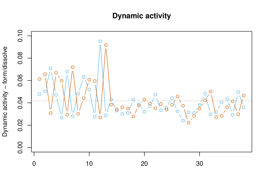
Figure 1: Evolution of edge density $D_{t}$ (left panel), percentage of grown $D_{1,t}$ (blue) and dissolved $D_{0,t}$ (orange) edges (right panel), manufacturing email networks.

We also identify empirical evidence in the data for transitivity effects. This is demonstrated in Figure 2. To construct these plots, we partition the edge variables as follows: for each integer $\ell\geq 0$, define

$$\mathcal{U}_{\ell}=\big{\{}(i,j,t):1\leq i<j\leq p\,,~{}t\in[n]\setminus\{1\}\,,~{}X_{i,j}^{t-1}=0\,,~{}U_{i,j}^{t-1}=\ell/(p-2)\big{\}}\,,$$

$$\mathcal{V}_{\ell}=\big{\{}(i,j,t):1\leq i<j\leq p\,,~{}t\in[n]\setminus\{1\}\,,~{}X_{i,j}^{t-1}=1\,,~{}V_{i,j}^{t-1}=\ell/(p-2)\big{\}}\,,$$

$$\mathcal{U}_{\ell}^{1}=\big{\{}(i,j,t)\in\mathcal{U}_{\ell},\;X_{i,j}^{t}=1\big{\}},\quad\mathcal{V}_{\ell}^{0}=\big{\{}(i,j,t)\in\mathcal{V}_{\ell},\;X_{i,j}^{t}=0\big{\}}\,,$$

where $U_{i,j}^{t-1}$ and $V_{i,j}^{t-1}$ are given in (3.4).

The left panel plots the relative frequency $|\mathcal{U}_{\ell}^{1}|\big{/}|\mathcal{U}_{\ell}|$ against $\ell$ for $\ell=0,1,\cdots$, showing that this frequency of grown edges tends to be higher for node pairs with more common neighbours in the previous snapshot. The right panel analogously plots the relative frequency $|\mathcal{V}_{\ell}^{0}|/\big{/}|\mathcal{V}_{\ell}|$ against $\ell$, and shows a similar increasing relationship between disjoint neighbours and frequency of dissolved edges.

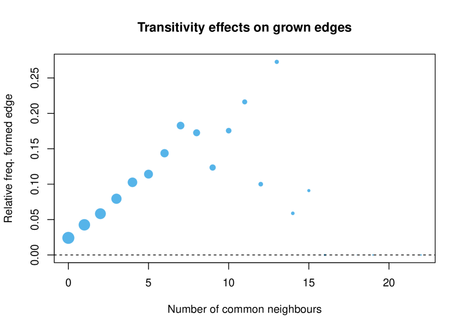
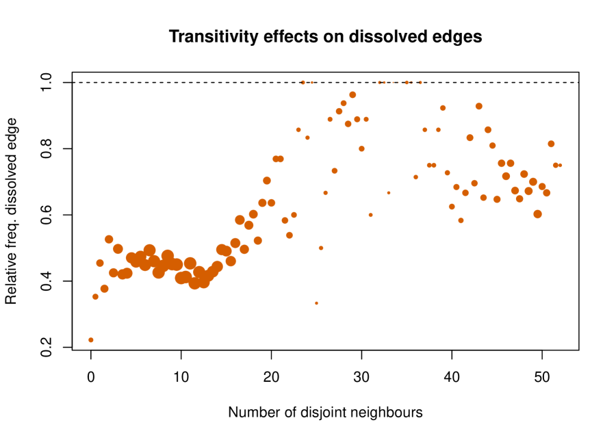
Figure 2: Left panel: the plot of relative edge frequency $|\mathcal{U}_{\ell}^{1}|\big{/}|\mathcal{U}_{\ell}|$ against $\ell$. Right panel: the plot of relative non-edge frequency $|\mathcal{V}_{\ell}^{0}|\big{/}|\mathcal{V}_{\ell}|$ against $\ell$. In both panels, point size is proportional to log$|\mathcal{U}_{\ell}|$ and log$|\mathcal{V}_{\ell}|$ respectively.

This is confirmed by the fit of our model parameters, using the estimation algorithm described in Section 4, and implemented in our development R package arnetworks. For period 1, we estimate the global parameters $\hat{a}=13.12$ and $\hat{b}=9.34$, suggesting a tendency towards edge growth given more common neighbours, and edge dissolution given more distinct neighbours, which agrees with the empirical evidence in Figure 2. We interpret the estimates of the local parameters $\{\xi_{i}\}_{i=1}^{106}$ and $\{\eta_{i}\}_{i=1}^{106}$ in the left panel of Figure 3. The estimates $\{\hat{\xi}_{i}\}_{i=1}^{106}$ have mean $0.61$ and skew towards the right, implying degree heterogeneity in the edge growth. Conversely, the estimates $\{\hat{\eta}_{i}\}_{i=1}^{106}$ have mean $0.89$ and skew towards the left. There is a decreasing relationship between the paired parameters: employees who tend to grow new edges also tend to maintain existing edges. Finally, there is an observed relationship between email behavior and company hierarchy: managers (non-leaf nodes in the organizational tree) tend to have larger estimates $\{\hat{\xi}_{i}\}_{i=1}^{106}$ compared to non-managers (means $0.74$ and $0.57$ respectively), implying that managers are more likely to grow edges. However, this increasing pattern does not continue at higher levels of the organizational tree.

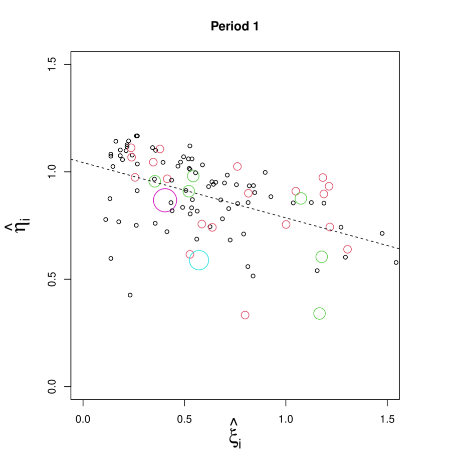
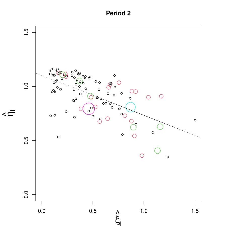
Figure 3: Scatter plots of estimates $\{\hat{\xi}_{i}\}_{i=1}^{106}$ and $\{\hat{\eta}_{i}\}_{i=1}^{106}$ for periods 1 and 2. Circles are sized and coloured according to their level in the company organizational tree. The smallest black circles have no direct reports, while the largest purple circle is the CEO.

The model fit to period 2 shows many of the same patterns. We estimate $\hat{a}=21.69$ and $\hat{b}=9.84$ and summarize the estimates $\{\hat{\xi}_{i}\}_{i=1}^{106}$ and $\{\hat{\eta}_{i}\}_{i=1}^{106}$ in the right panel of Figure 3. Relative to period 1, the larger estimate of $a$ implies a stronger transitivity effect in this time period. The estimates $\{\hat{\xi}_{i}\}_{i=1}^{106}$ now have mean $0.49$ and the estimates $\{\hat{\eta}_{i}\}_{i=1}^{106}$ have mean $0.92$, to model overall lower edge density. The decreasing relationship between the paired parameters is stronger, and the means of ${\hat{\xi}_{i}}$ for managers and non-managers are, respectively, $0.68$ and $0.43$. Along with the stronger transitivity effect, we interpret that the decreased network density in period 2 has led to a concentration of email activity among a smaller group of employees, many of them managers.

We compare our model to some competing models from the literature in terms of Akaike and Bayesian information criteria (AIC, BIC). To briefly describe these competitors: the “global AR model” and “edgewise AR model” fit the model of Jiang et al. (2023b), with either two global switching parameters or two parameters for each edge. The “edgewise mean model” assumes

$$X_{i,j}^{t}\overset{\mathrm{iid}}{\sim}\operatorname{Bernoulli}(P_{i,j})$$

with no temporal dependence, and estimates the edge probability $\{P_{i,j}\}_{i,j:\,i<j}$ for each node pair by its relative frequency in the training set; and the “degree parameter mean model” assumes

$$X_{i,j}^{t}\overset{\mathrm{iid}}{\sim}\operatorname{Bernoulli}(\nu_{i}\nu_{j})$$

and estimates the degree parameters $\{\nu_{i}\}_{i=1}^{106}$ by fitting 1-dimensional adjacency spectral embedding (Athreya et al., 2017) to the mean adjacency matrix over the training set. Note that the edgewise mean model has $O(p^{2})$ parameters, while the degree parameter model has $O(p)$ parameters like our AR network model with transitivity. All of these models can be directly compared using the AR network model likelihood, although only our AR network model with transitivity incorporates edge dependence, and the final two models do not incorporate any temporal dependence. Results for both regimes are reported in Table 2.

	Period 1		Period 2
Model	AIC	BIC	AIC	BIC
Transitivity AR model	33226	35175	52547	54654
Global AR model	36309	36327	58267	58287
Edgewise AR model	42717	144102	55840	165394
Edgewise mean model	33248	83941	47133	101910
Degree parameter mean model	41730	42695	68969	70013

Table 2: AIC and BIC performance for email interaction data, periods 1 and 2.

In period 1, our AR network model with transitivity achieves the lowest AIC and BIC, while in period 2 it is outperformed slightly by the edgewise mean model in terms of AIC, but achieves a lower BIC as it uses fewer parameters. This reduction of the parameter space is important for modeling sparse dynamic network data: although there is clear temporal edge dependence in this data, the edgewise mean model outperforms the edgewise AR model, as there is low effective sample size to estimate the edge dissolution parameters.

Finally, we compare the performances of those models in an edge forecasting task on the final 26 network snapshots (period 2). For $n_{\mathrm{train}}=10,\ldots,23$, we train these models on the first $n_{\mathrm{train}}$ snapshots of period 2, then forecast the state of each edge $n_{\mathrm{step}}$ steps forward, for $n_{\mathrm{step}}=1,2,3$. The combined results are presented in Figure 4 as receiver operating characteristic (ROC) curves. We also include a single point summarizing the naive forecasting performance using the most recent observation of that edge in the training set.

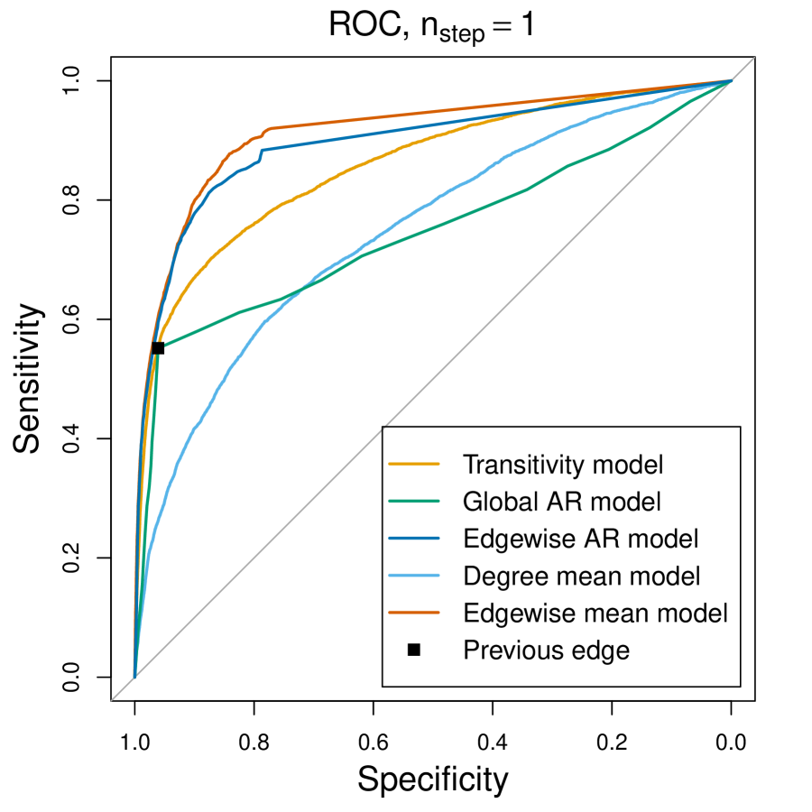
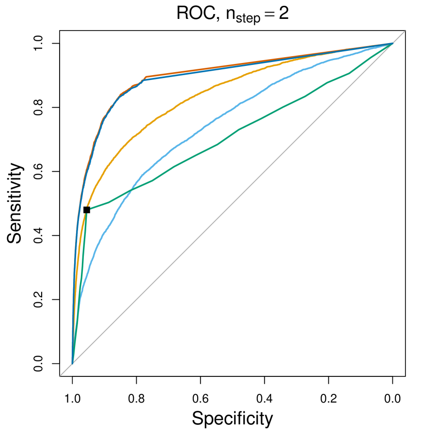
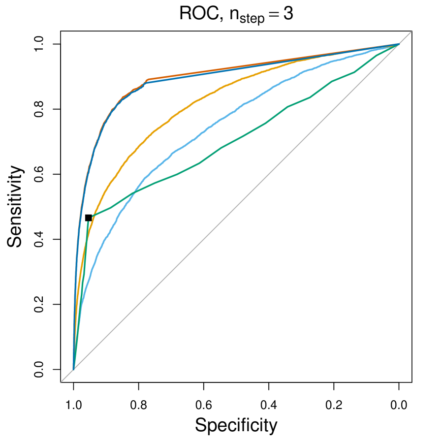
Figure 4: ROC curves for link prediction performance, email interaction data.

Our AR network model with transitivity dominates or is competitive with all the models besides these highly parameterized edgewise models for all choices of $n_{\mathrm{step}}$. The good performance of the edgewise models suggests the presence of higher order structure in this network that cannot be modeled with only two parameters per node. Note that the edgewise mean and edgewise AR models give very similar, but not identical edge predictions; as mentioned above, due to network sparsity the edgewise AR model has a low effective sample size to estimate the dissolution parameters, leading to slightly worse link prediction performance.

Supplementary material to “Autoregressive Networks with Dependent Edges”

Jinyuan Chang, Qin Fang, Eric D. Kolaczyk, Peter W. MacDonald, and Qiwei Yao

This supplementary material contains a detailed analysis on the relationship between the proposed AR models and temporal ERGMs (Section A), all the technical proofs (Section B), additional numerical simulation results (Section C), and the analysis of an additional dynamic network dataset (Section D).

Appendix A Relationship to temporal ERGMs

A dynamic network sequence follows a temporal ERGM of order $m$ if it satisfies

$$\mathbb{P}({\bf X}_{t}\,|\,{\bf X}_{t-1},\ldots,{\bf X}_{t-m};\boldsymbol{\theta})\propto\exp\{\boldsymbol{\varsigma}(\boldsymbol{\theta})^{{\scriptscriptstyle\top}}\boldsymbol{\varrho}({\bf X}_{t},{\bf X}_{t-1},\ldots,{\bf X}_{t-m})\}\,,$$ (A.1)

where $\boldsymbol{\varsigma}:\mathbb{R}^{q}\rightarrow\mathbb{R}^{p}$ maps the parameter vector $\boldsymbol{\theta}$ to the vector of natural parameters, and $\boldsymbol{\varrho}$ maps the data, including the past network snapshots, to the corresponding sufficient statistics.

As in Equation (2) of Hanneke et al. (2010), suppose $\boldsymbol{\varrho}$ factors over the edges of the present snapshot,

$$\boldsymbol{\varrho}({\bf X}_{t},{\bf X}_{t-1},\ldots,{\bf X}_{t-m})=\sum_{i,j:\,i<j}\boldsymbol{\varrho}_{i,j}(X^{t}_{i,j};{\bf X}_{t-1},\ldots,{\bf X}_{t-m})\,.$$

Then

$$\mathbb{P}({\bf X}_{t}\,|\,{\bf X}_{t-1},\ldots,{\bf X}_{t-m};\boldsymbol{\theta})$$

$$~{}~{}~{}~{}~{}~{}~{}~{}~{}~{}~{}~{}~{}~{}~{}~{}\propto\prod_{i,j:\,i<j}\exp\big{\{}\boldsymbol{\varsigma}(\boldsymbol{\theta})^{{\scriptscriptstyle\top}}\boldsymbol{\varrho}_{i,j}(X^{t}_{i,j};X_{i,j}^{t-1},{\bf X}_{t-1}\setminus X_{i,j}^{t-1},{\bf X}_{t-2},\ldots,{\bf X}_{t-m})\big{\}}\,,$$ (A.2)

which implies ${\bf X}_{t}$ will have mutually independent edges conditional on the past snapshots. We refer to this as the edge conditional independence assumption, which is a property of AR network models defined in Definition 1 of the main document. We will show that any edge conditionally independent temporal ERGM can be rewritten as an AR network model.

Denote the logit function by $\sigma(x)=\log\{x/(1-x)\}$, and specify an AR network model defined in Definition 1 by setting

$$\alpha_{i,j}^{t-1}= ~{}\sigma^{-1}\big{[}\boldsymbol{\varsigma}(\boldsymbol{\theta})^{{\scriptscriptstyle\top}}\big{\{}\boldsymbol{\varrho}_{i,j}(1;0,{\bf X}_{t-1}\setminus X_{i,j}^{t-1},{\bf X}_{t-2},\ldots,{\bf X}_{t-m})$$

$$~{}~{}~{}~{}~{}~{}~{}~{}~{}~{}~{}~{}~{}~{}~{}~{}~{}~{}~{}~{}~{}~{}~{}~{}~{}-\boldsymbol{\varrho}_{i,j}(0;0,{\bf X}_{t-1}\setminus X_{i,j}^{t-1},{\bf X}_{t-2},\ldots,{\bf X}_{t-m})\big{\}}\big{]}$$

$$:= ~{}\sigma^{-1}[\boldsymbol{\varsigma}(\boldsymbol{\theta})^{{\scriptscriptstyle\top}}(\boldsymbol{\varrho}_{i,j,10}^{t-1}-\boldsymbol{\varrho}_{i,j,00}^{t-1})]\,,$$ (A.3)

$$\beta_{i,j}^{t-1}= ~{}\sigma^{-1}\big{[}\boldsymbol{\varsigma}(\boldsymbol{\theta})^{{\scriptscriptstyle\top}}\big{\{}\boldsymbol{\varrho}_{i,j}(0;1,{\bf X}_{t-1}\setminus X_{i,j}^{t-1},{\bf X}_{t-2},\ldots,{\bf X}_{t-m})$$

$$~{}~{}~{}~{}~{}~{}~{}~{}~{}~{}~{}~{}~{}~{}~{}~{}~{}~{}~{}~{}~{}~{}~{}~{}~{}-\boldsymbol{\varrho}_{i,j}(1;1,{\bf X}_{t-1}\setminus X_{i,j}^{t-1},{\bf X}_{t-2},\ldots,{\bf X}_{t-m})\big{\}}\big{]}$$

$$:= ~{}\sigma^{-1}[\boldsymbol{\varsigma}(\boldsymbol{\theta})^{{\scriptscriptstyle\top}}(\boldsymbol{\varrho}_{i,j,01}^{t-1}-\boldsymbol{\varrho}_{i,j,11}^{t-1})]\,.$$ (A.4)

With renormalizing, we have

$$\alpha_{i,j}^{t-1} =\frac{\exp\{\boldsymbol{\varsigma}(\boldsymbol{\theta})^{{\scriptscriptstyle\top}}\boldsymbol{\varrho}_{i,j,10}^{t-1}\}}{\exp\{\boldsymbol{\varsigma}(\boldsymbol{\theta})^{{\scriptscriptstyle\top}}\boldsymbol{\varrho}_{i,j,10}^{t-1}\}+\exp\{\boldsymbol{\varsigma}(\boldsymbol{\theta})^{{\scriptscriptstyle\top}}\boldsymbol{\varrho}_{i,j,00}^{t-1}\}}\,,$$

$$1-\alpha_{i,j}^{t-1} =\frac{\exp\{\boldsymbol{\varsigma}(\boldsymbol{\theta})^{{\scriptscriptstyle\top}}\boldsymbol{\varrho}_{i,j,00}^{t-1}\}}{\exp\{\boldsymbol{\varsigma}(\boldsymbol{\theta})^{{\scriptscriptstyle\top}}\boldsymbol{\varrho}_{i,j,10}^{t-1}\}+\exp\{\boldsymbol{\varsigma}(\boldsymbol{\theta})^{{\scriptscriptstyle\top}}\boldsymbol{\varrho}_{i,j,00}^{t-1}\}}\,,$$

$$\beta_{i,j}^{t-1} =\frac{\exp\{\boldsymbol{\varsigma}(\boldsymbol{\theta})^{{\scriptscriptstyle\top}}\boldsymbol{\varrho}_{i,j,01}^{t-1}\}}{\exp\{\boldsymbol{\varsigma}(\boldsymbol{\theta})^{{\scriptscriptstyle\top}}\boldsymbol{\varrho}_{i,j,01}^{t-1}\}+\exp\{\boldsymbol{\varsigma}(\boldsymbol{\theta})^{{\scriptscriptstyle\top}}\boldsymbol{\varrho}_{i,j,11}^{t-1}\}}\,,$$

$$1-\beta_{i,j}^{t-1} =\frac{\exp\{\boldsymbol{\varsigma}(\boldsymbol{\theta})^{{\scriptscriptstyle\top}}\boldsymbol{\varrho}_{i,j,11}^{t-1}\}}{\exp\{\boldsymbol{\varsigma}(\boldsymbol{\theta})^{{\scriptscriptstyle\top}}\boldsymbol{\varrho}_{i,j,01}^{t-1}\}+\exp\{\boldsymbol{\varsigma}(\boldsymbol{\theta})^{{\scriptscriptstyle\top}}\boldsymbol{\varrho}_{i,j,11}^{t-1}\}}\,.$$

For the AR network model with $(\alpha_{i,j}^{t-1},\beta_{i,j}^{t-1})$ specified in (A.3) and (A.4), it holds that

$$\mathbb{P}({\bf X}_{t}\,|\,{\bf X}_{t-1},\ldots,{\bf X}_{t-m};\boldsymbol{\theta})=\prod_{i,j:\,i<j}\mathbb{P}(X_{i,j}^{t}\,|\,{\bf X}_{t-1},\ldots,{\bf X}_{t-m};\boldsymbol{\theta})$$

$$~{}~{}~{}~{}~{}=\prod_{i,j:\,i<j,\,X_{i,j}^{t}=0,\,X_{i,j}^{t-1}=0}(1-\alpha_{i,j}^{t-1})\cdot\prod_{i,j:\,i<j,\,X_{i,j}^{t}=1,\,X_{i,j}^{t-1}=0}\alpha_{i,j}^{t-1}$$

$$~{}~{}~{}~{}~{}~{}~{}~{}~{}~{}~{}~{}~{}~{}~{}\cdot\prod_{i,j:\,i<j,\,X_{i,j}^{t}=0,\,X_{i,j}^{t-1}=1}\beta_{i,j}^{t-1}\cdot\prod_{i,j:\,i<j,\,X_{i,j}^{t}=1,\,X_{i,j}^{t-1}=1}(1-\beta_{i,j}^{t-1})$$

$$~{}~{}~{}~{}~{}~{}\propto\prod_{i,j:\,i<j,\,X_{i,j}^{t}=0,\,X_{i,j}^{t-1}=0}\exp\{\boldsymbol{\varsigma}(\boldsymbol{\theta})^{{\scriptscriptstyle\top}}\boldsymbol{\varrho}_{i,j,00}^{t-1}\}\cdot\prod_{i,j:\,i<j,\,X_{i,j}^{t}=1,\,X_{i,j}^{t-1}=0}\exp\{\boldsymbol{\varsigma}(\boldsymbol{\theta})^{{\scriptscriptstyle\top}}\boldsymbol{\varrho}_{i,j,10}^{t-1}\}$$

$$~{}~{}~{}~{}~{}~{}~{}~{}~{}~{}~{}~{}~{}~{}~{}\cdot\prod_{i,j:\,i<j,\,X_{i,j}^{t}=0,\,X_{i,j}^{t-1}=1}\exp\{\boldsymbol{\varsigma}(\boldsymbol{\theta})^{{\scriptscriptstyle\top}}\boldsymbol{\varrho}_{i,j,01}^{t-1}\}\cdot\prod_{i,j:\,i<j,\,X_{i,j}^{t}=1,\,X_{i,j}^{t-1}=1}\exp\{\boldsymbol{\varsigma}(\boldsymbol{\theta})^{{\scriptscriptstyle\top}}\boldsymbol{\varrho}_{i,j,11}^{t-1}\}$$

$$~{}~{}~{}~{}~{}=\prod_{i,j:\,i<j}\exp\big{\{}\boldsymbol{\varsigma}(\boldsymbol{\theta})^{{\scriptscriptstyle\top}}\boldsymbol{\varrho}_{i,j}(X^{t}_{i,j};X_{i,j}^{t-1},{\bf X}_{t-1}\setminus X_{i,j}^{t-1},{\bf X}_{t-2},\ldots,{\bf X}_{t-m})\big{\}}\,,$$

which shares the same form as (A.2). Thus for any edge conditionally independent temporal ERGM, we can specify an AR network model with the same distribution.

Conversely, suppose we have specified an AR network model such that

$$\sigma(\alpha_{i,j}^{t-1}) =\boldsymbol{\phi}(\boldsymbol{\theta})^{{\scriptscriptstyle\top}}{\mathbf{u}}_{i,j}({\bf X}_{t-1}\setminus X_{i,j}^{t-1},{\bf X}_{t-2},\ldots,{\bf X}_{t-m})\,,$$

$$\sigma(\beta_{i,j}^{t-1}) =\boldsymbol{\psi}(\boldsymbol{\theta})^{{\scriptscriptstyle\top}}{\mathbf{v}}_{i,j}({\bf X}_{t-1}\setminus X_{i,j}^{t-1},{\bf X}_{t-2},\ldots,{\bf X}_{t-m})\,,$$

for some functions of the parameter vector $\boldsymbol{\theta}$, and the past network behavior. We claim that this AR network model can be written as an edge conditionally independent temporal ERGM (A.1) with $\boldsymbol{\varsigma}(\boldsymbol{\theta})=(\boldsymbol{\phi}(\boldsymbol{\theta})^{{\scriptscriptstyle\top}},\boldsymbol{\psi}(\boldsymbol{\theta})^{{\scriptscriptstyle\top}})^{{\scriptscriptstyle\top}}$ and $\boldsymbol{\varrho}({\bf X}_{t},{\bf X}_{t-1},\ldots,{\bf X}_{t-m})=(\boldsymbol{\varrho}_{\alpha}^{{\scriptscriptstyle\top}},\boldsymbol{\varrho}_{\beta}^{{\scriptscriptstyle\top}})^{{\scriptscriptstyle\top}}$, where $\boldsymbol{\varrho}_{\alpha}=\sum_{i,j:\,i<j}\boldsymbol{\varrho}_{\alpha,i,j}$ and $\boldsymbol{\varrho}_{\beta}=\sum_{i,j:\,i<j}\boldsymbol{\varrho}_{\beta,i,j}$ with

$$\boldsymbol{\varrho}_{\alpha,i,j}(X_{i,j}^{t};X_{i,j}^{t-1},{\bf X}_{t-1}\setminus X_{i,j}^{t-1},{\bf X}_{t-2},\ldots,{\bf X}_{t-m})$$

$$~{}~{}~{}~{}~{}~{}~{}~{}~{}={\mathbf{u}}_{i,j}({\bf X}_{t-1}\setminus X_{i,j}^{t-1},{\bf X}_{t-2},\ldots,{\bf X}_{t-m})I(X_{i,j}^{t}=1,X_{i,j}^{t-1}=0)\,,$$

$$\boldsymbol{\varrho}_{\beta,i,j}(X_{i,j}^{t};X_{i,j}^{t-1},{\bf X}_{t-1}\setminus X_{i,j}^{t-1},{\bf X}_{t-2},\ldots,{\bf X}_{t-m})$$

$$~{}~{}~{}~{}~{}~{}~{}~{}~{}={\mathbf{v}}_{i,j}({\bf X}_{t-1}\setminus X_{i,j}^{t-1},{\bf X}_{t-2},\ldots,{\bf X}_{t-m})I(X_{i,j}^{t}=0,X_{i,j}^{t-1}=1)\,.$$

Krivitsky and Handcock (2014) define the concept of separability of a dynamic model for binary networks. Define two subnetworks ${\bf X}^{+}_{t}$ and ${\bf X}^{-}_{t}$, where

$$X_{i,j}^{t,+} =1-I(X_{i,j}^{t}=0,X_{i,j}^{t-1}=0),$$

$$X_{i,j}^{t,-} =I(X_{i,j}^{t}=1,X_{i,j}^{t-1}=1),$$

for all $i,j$. A dynamic network model is said to be separable if ${\bf X}^{+}_{t}$ and ${\bf X}^{-}_{t}$ are independent conditional on the past, and do not share any parameters. In particular, a separable temporal ERGM (STERGM) can be specified by a product of a formation model and a dissolution model:

$$\mathbb{P}({\bf X}_{t}\,|\,{\bf X}_{t-1},\ldots,{\bf X}_{t-m};\boldsymbol{\theta})$$

$$~{}~{}~{}~{}~{}~{}\propto\exp\big{\{}\boldsymbol{\varsigma}^{+}(\boldsymbol{\theta}^{+})^{{\scriptscriptstyle\top}}\boldsymbol{\varrho}^{+}({\bf X}^{+}_{t},{\bf X}_{t-1},\ldots,{\bf X}_{t-m})+\boldsymbol{\varsigma}^{-}(\boldsymbol{\theta}^{-})^{{\scriptscriptstyle\top}}\boldsymbol{\varrho}^{-}({\bf X}_{t}^{-},{\bf X}_{t-1},\ldots,{\bf X}_{t-m})\big{\}}\,,$$ (A.5)

where $\boldsymbol{\varsigma}^{+}$ and $\boldsymbol{\varsigma}^{-}$ map parameter vectors $\boldsymbol{\theta}^{+}$ and $\boldsymbol{\theta}^{-}$ to the vectors of natural parameters, and $\boldsymbol{\varrho}^{+}$ and $\boldsymbol{\varrho}^{-}$ map the data, including the past network snapshots, to the corresponding sufficient statistics.

Under the edge conditional independence assumption, we can write

$$\boldsymbol{\varrho}^{+}({\bf X}^{+}_{t},{\bf X}_{t-1},\ldots,{\bf X}_{t-m})=\sum_{i<j}\boldsymbol{\varrho}_{i,j}^{+}(X_{i,j}^{t,+};X_{i,j}^{t-1},{\bf X}_{t-1}\setminus X_{i,j}^{t-1},\ldots,{\bf X}_{t-m}),$$

or equivalently

$$\boldsymbol{\varrho}^{+}({\bf X}^{+}_{t},{\bf X}_{t-1},\ldots,{\bf X}_{t-m})=\sum_{i<j}\tilde{\boldsymbol{\varrho}}_{i,j}^{+}(X_{i,j}^{t};X_{i,j}^{t-1},{\bf X}_{t-1}\setminus X_{i,j}^{t-1},\ldots,{\bf X}_{t-m}),$$

since for all $i<j$, $X_{i,j}^{t,+}$ can be recovered from $X_{i,j}^{t}$ and $X_{i,j}^{t-1}$. Define $\tilde{\boldsymbol{\varrho}}^{-}_{i,j}$ analogously for the dissolution model.

In this way $X_{t}$ is an edge conditionally independent TERGM with parameter vector $(\boldsymbol{\theta}^{+},\boldsymbol{\theta}^{-})$, natural parameter

$$(\varsigma^{+}(\boldsymbol{\theta}^{+}),\varsigma^{-}(\boldsymbol{\theta}^{-})),$$

and sufficient statistic

$$\left(\sum_{i<j}\tilde{\boldsymbol{\varrho}}^{+}_{i,j},\sum_{i<j}\tilde{\boldsymbol{\varrho}}^{-}_{i,j}\right).$$

Following the above construction to rewrite this as an AR network model, we can write

$$\alpha_{i,j}^{t-1}= ~{}\sigma^{-1}\big{[}\boldsymbol{\varsigma}^{+}(\boldsymbol{\theta}^{+})^{{\scriptscriptstyle\top}}\big{\{}\tilde{\boldsymbol{\varrho}}^{+}_{i,j}(1;0,{\bf X}_{t-1}\setminus X_{i,j}^{t-1},{\bf X}_{t-2},\ldots,{\bf X}_{t-m})$$

$$~{}~{}~{}~{}~{}~{}~{}~{}~{}~{}~{}~{}~{}~{}~{}~{}-\tilde{\boldsymbol{\varrho}}^{+}_{i,j}(0;0,{\bf X}_{t-1}\setminus X_{i,j}^{t-1},{\bf X}_{t-2},\ldots,{\bf X}_{t-m})\big{\}}$$

$$~{}~{}~{}+\boldsymbol{\varsigma}^{-}(\boldsymbol{\theta}^{-})^{{\scriptscriptstyle\top}}\big{\{}\tilde{\boldsymbol{\varrho}}^{-}_{i,j}(1;0,{\bf X}_{t-1}\setminus X_{i,j}^{t-1},{\bf X}_{t-2},\ldots,{\bf X}_{t-m})$$

$$~{}~{}~{}~{}~{}~{}~{}~{}~{}~{}~{}~{}~{}~{}~{}~{}-\tilde{\boldsymbol{\varrho}}^{-}_{i,j}(0;0,{\bf X}_{t-1}\setminus X_{i,j}^{t-1},{\bf X}_{t-2},\ldots,{\bf X}_{t-m})\big{\}}\big{]},$$

and note that

$$\tilde{\boldsymbol{\varrho}}^{-}_{i,j}(1;0,{\bf X}_{t-1}\setminus X_{i,j}^{t-1},{\bf X}_{t-2},\ldots,{\bf X}_{t-m}) =\tilde{\boldsymbol{\varrho}}^{-}_{i,j}(0;0,{\bf X}_{t-1}\setminus X_{i,j}^{t-1},{\bf X}_{t-2},\ldots,{\bf X}_{t-m})$$

$$=\boldsymbol{\varrho}^{-}_{i,j}(0;0,{\bf X}_{t-1}\setminus X_{i,j}^{t-1},{\bf X}_{t-2},\ldots,{\bf X}_{t-m})$$

for all $i<j$ and $t$, since $X_{i,j}^{t,-}=0$ whenever $X_{i,j}^{t-1}=0$. Thus $\alpha_{i,j}^{t-1}$ is free of $\boldsymbol{\theta}^{-}$. Similarly, we can write

$$\beta_{i,j}^{t-1}= ~{}\sigma^{-1}\big{[}\boldsymbol{\varsigma}^{+}(\boldsymbol{\theta}^{+})^{{\scriptscriptstyle\top}}\big{\{}\tilde{\boldsymbol{\varrho}}^{+}_{i,j}(0;1,{\bf X}_{t-1}\setminus X_{i,j}^{t-1},{\bf X}_{t-2},\ldots,{\bf X}_{t-m})$$

$$~{}~{}~{}~{}~{}~{}~{}~{}~{}~{}~{}~{}~{}~{}~{}~{}-\tilde{\boldsymbol{\varrho}}^{+}_{i,j}(1;1,{\bf X}_{t-1}\setminus X_{i,j}^{t-1},{\bf X}_{t-2},\ldots,{\bf X}_{t-m})\big{\}}$$

$$~{}~{}~{}+\boldsymbol{\varsigma}^{-}(\boldsymbol{\theta}^{-})^{{\scriptscriptstyle\top}}\big{\{}\tilde{\boldsymbol{\varrho}}^{-}_{i,j}(0;1,{\bf X}_{t-1}\setminus X_{i,j}^{t-1},{\bf X}_{t-2},\ldots,{\bf X}_{t-m})$$

$$~{}~{}~{}~{}~{}~{}~{}~{}~{}~{}~{}~{}~{}~{}~{}~{}-\tilde{\boldsymbol{\varrho}}^{-}_{i,j}(1;1,{\bf X}_{t-1}\setminus X_{i,j}^{t-1},{\bf X}_{t-2},\ldots,{\bf X}_{t-m})\big{\}}\big{]},$$

and

$$\tilde{\boldsymbol{\varrho}}^{+}_{i,j}(0;1,{\bf X}_{t-1}\setminus X_{i,j}^{t-1},{\bf X}_{t-2},\ldots,{\bf X}_{t-m}) =\tilde{\boldsymbol{\varrho}}^{+}_{i,j}(1;1,{\bf X}_{t-1}\setminus X_{i,j}^{t-1},{\bf X}_{t-2},\ldots,{\bf X}_{t-m})$$

$$=\boldsymbol{\varrho}^{+}_{i,j}(1;1,{\bf X}_{t-1}\setminus X_{i,j}^{t-1},{\bf X}_{t-2},\ldots,{\bf X}_{t-m})$$

for all $i<j$ and $t$, since $X_{i,j}^{t,+}=1$ whenever $X_{i,j}^{t-1}=1$. Then $\beta_{i,j}^{t-1}$ is free of $\boldsymbol{\theta}^{+}$. Hence any edge conditionally independent STERGM can be written as an AR network model with separable parameters.

Conversely, suppose we have specified an AR network model such that

$$\sigma(\alpha_{i,j}^{t-1}) =\boldsymbol{\phi}(\boldsymbol{\theta}_{\alpha})^{{\scriptscriptstyle\top}}{\mathbf{u}}_{i,j}({\bf X}_{t-1}\setminus X_{i,j}^{t-1},{\bf X}_{t-2},\ldots,{\bf X}_{t-m})$$

$$\sigma(\beta_{i,j}^{t-1}) =\boldsymbol{\psi}(\boldsymbol{\theta}_{\beta})^{{\scriptscriptstyle\top}}{\mathbf{v}}_{i,j}({\bf X}_{t-1}\setminus X_{i,j}^{t-1},{\bf X}_{t-2},\ldots,{\bf X}_{t-m})$$

with separable parameters $\boldsymbol{\theta}_{\alpha}$ and $\boldsymbol{\theta}_{\beta}$.

We follow the same construction as above to rewrite this model as an edge conditionally independent TERGM, with parameter vector $\boldsymbol{\varsigma}(\boldsymbol{\theta})=(\boldsymbol{\phi}(\boldsymbol{\theta}_{\alpha})^{{\scriptscriptstyle\top}},\boldsymbol{\psi}(\boldsymbol{\theta}_{\beta})^{{\scriptscriptstyle\top}})^{{\scriptscriptstyle\top}}$ and sufficient statistics $\boldsymbol{\varrho}({\bf X}_{t},{\bf X}_{t-1},\ldots,{\bf X}_{t-m})=(\boldsymbol{\varrho}_{\alpha}^{{\scriptscriptstyle\top}},\boldsymbol{\varrho}_{\beta}^{{\scriptscriptstyle\top}})^{{\scriptscriptstyle\top}}$, where $\boldsymbol{\varrho}_{\alpha}=\sum_{i,j:\,i<j}\boldsymbol{\varrho}_{\alpha,i,j}$ and $\boldsymbol{\varrho}_{\beta}=\sum_{i,j:\,i<j}\boldsymbol{\varrho}_{\beta,i,j}$ with

$$\boldsymbol{\varrho}_{\alpha,i,j}(X_{i,j}^{t};X_{i,j}^{t-1},{\bf X}_{t-1}\setminus X_{i,j}^{t-1},{\bf X}_{t-2},\ldots,{\bf X}_{t-m})$$

$$~{}~{}~{}~{}~{}~{}~{}~{}~{}={\mathbf{u}}_{i,j}({\bf X}_{t-1}\setminus X_{i,j}^{t-1},{\bf X}_{t-2},\ldots,{\bf X}_{t-m})I(X_{i,j}^{t}=1,X_{i,j}^{t-1}=0)\,,$$

$$~{}~{}~{}~{}~{}~{}~{}~{}~{}={\mathbf{u}}_{i,j}({\bf X}_{t-1}\setminus X_{i,j}^{t-1},{\bf X}_{t-2},\ldots,{\bf X}_{t-m})I(X_{i,j}^{t,+}=1,X_{i,j}^{t-1}=0)\,,$$ (A.6)

$$\boldsymbol{\varrho}_{\beta,i,j}(X_{i,j}^{t};X_{i,j}^{t-1},{\bf X}_{t-1}\setminus X_{i,j}^{t-1},{\bf X}_{t-2},\ldots,{\bf X}_{t-m})$$

$$~{}~{}~{}~{}~{}~{}~{}~{}~{}={\mathbf{v}}_{i,j}({\bf X}_{t-1}\setminus X_{i,j}^{t-1},{\bf X}_{t-2},\ldots,{\bf X}_{t-m})I(X_{i,j}^{t}=0,X_{i,j}^{t-1}=1)\,.$$

$$~{}~{}~{}~{}~{}~{}~{}~{}~{}={\mathbf{v}}_{i,j}({\bf X}_{t-1}\setminus X_{i,j}^{t-1},{\bf X}_{t-2},\ldots,{\bf X}_{t-m})I(X_{i,j}^{t,-}=0,X_{i,j}^{t-1}=1)\,.$$ (A.7)

Note that in (A.6) and (A.7), the sufficient statistics depend on $X_{i,j}^{t}$ only through $X_{i,j}^{t,+}$ and $X_{i,j}^{t,-}$ respectively. It follows that when written as a conditionally independent TERGM, the distribution factors into a product of a formation model and dissolution model, as in (A.5). Thus this AR network model is an edge conditionally independent STERGM.

Appendix B Technical proofs

B.1 Proof of Proposition 1

Recall

$$\ell_{n,p}^{(l)}(\boldsymbol{\theta})=\frac{1}{(n-m)|\mathcal{S}_{l}|}\sum_{t=m+1}^{n}\sum_{(i,j)\in\mathcal{S}_{l}}h_{i,j}^{t-1}(\boldsymbol{\theta})$$

with

$$h_{i,j}^{t-1}(\boldsymbol{\theta})=\log\{1-\gamma_{i,j}^{t-1}(\boldsymbol{\theta})\}+\gamma_{i,j}^{t-1}(\boldsymbol{\theta}_{0})\log\bigg{\{}\frac{\gamma_{i,j}^{t-1}(\boldsymbol{\theta})}{1-\gamma_{i,j}^{t-1}(\boldsymbol{\theta})}\bigg{\}}\,.$$

Then

$$\frac{\partial h_{i,j}^{t-1}(\boldsymbol{\theta})}{\partial\theta_{l_{1}}}= ~{}\frac{\gamma_{i,j}^{t-1}(\boldsymbol{\theta}_{0})-\gamma_{i,j}^{t-1}(\boldsymbol{\theta})}{\gamma_{i,j}^{t-1}(\boldsymbol{\theta})\{1-\gamma_{i,j}^{t-1}(\boldsymbol{\theta})\}}\frac{\partial\gamma_{i,j}^{t-1}(\boldsymbol{\theta})}{\partial\theta_{l_{1}}}\,,$$ (B.1)

$$\frac{\partial^{2}h_{i,j}^{t-1}(\boldsymbol{\theta})}{\partial\theta_{l_{1}}\partial\theta_{l_{2}}}= -\bigg{[}\frac{1}{\gamma_{i,j}^{t-1}(\boldsymbol{\theta})\{1-\gamma_{i,j}^{t-1}(\boldsymbol{\theta})\}}+\frac{\{\gamma_{i,j}^{t-1}(\boldsymbol{\theta}_{0})-\gamma_{i,j}^{t-1}(\boldsymbol{\theta})\}\{1-2\gamma_{i,j}^{t-1}(\boldsymbol{\theta})\}}{\{\gamma_{i,j}^{t-1}(\boldsymbol{\theta})\}^{2}\{1-\gamma_{i,j}^{t-1}(\boldsymbol{\theta})\}^{2}}\bigg{]}$$

$$~{}~{}~{}~{}~{}\times\frac{\partial\gamma_{i,j}^{t-1}(\boldsymbol{\theta})}{\partial\theta_{l_{1}}}\frac{\partial\gamma_{i,j}^{t-1}(\boldsymbol{\theta})}{\partial\theta_{l_{2}}}$$ (B.2)

$$+\frac{\gamma_{i,j}^{t-1}(\boldsymbol{\theta}_{0})-\gamma_{i,j}^{t-1}(\boldsymbol{\theta})}{\gamma_{i,j}^{t-1}(\boldsymbol{\theta})\{1-\gamma_{i,j}^{t-1}(\boldsymbol{\theta})\}}\frac{\partial^{2}\gamma_{i,j}^{t-1}(\boldsymbol{\theta})}{\partial\theta_{l_{1}}\partial\theta_{l_{2}}}\,,$$

$$\frac{\partial^{3}h_{i,j}^{t-1}(\boldsymbol{\theta})}{\partial\theta_{l_{1}}\partial\theta_{l_{2}}\partial\theta_{l_{3}}}= ~{}2\bigg{[}\frac{1-2\gamma_{i,j}^{t-1}(\boldsymbol{\theta})}{\{\gamma_{i,j}^{t-1}(\boldsymbol{\theta})\}^{2}\{1-\gamma_{i,j}^{t-1}(\boldsymbol{\theta})\}^{2}}+\frac{\gamma_{i,j}^{t-1}(\boldsymbol{\theta}_{0})-\gamma_{i,j}^{t-1}(\boldsymbol{\theta})}{\{\gamma_{i,j}^{t-1}(\boldsymbol{\theta})\}^{2}\{1-\gamma_{i,j}^{t-1}(\boldsymbol{\theta})\}^{2}}$$

$$~{}~{}~{}~{}~{}+\frac{\{\gamma_{i,j}^{t-1}(\boldsymbol{\theta}_{0})-\gamma_{i,j}^{t-1}(\boldsymbol{\theta})\}\{1-2\gamma_{i,j}^{t-1}(\boldsymbol{\theta})\}^{2}}{\{\gamma_{i,j}^{t-1}(\boldsymbol{\theta})\}^{3}\{1-\gamma_{i,j}^{t-1}(\boldsymbol{\theta})\}^{3}}\bigg{]}\frac{\partial\gamma_{i,j}^{t-1}(\boldsymbol{\theta})}{\partial\theta_{l_{1}}}\frac{\partial\gamma_{i,j}^{t-1}(\boldsymbol{\theta})}{\partial\theta_{l_{2}}}\frac{\partial\gamma_{i,j}^{t-1}(\boldsymbol{\theta})}{\partial\theta_{l_{3}}}$$

$$-\bigg{[}\frac{1}{\gamma_{i,j}^{t-1}(\boldsymbol{\theta})\{1-\gamma_{i,j}^{t-1}(\boldsymbol{\theta})\}}+\frac{\{\gamma_{i,j}^{t-1}(\boldsymbol{\theta}_{0})-\gamma_{i,j}^{t-1}(\boldsymbol{\theta})\}\{1-2\gamma_{i,j}^{t-1}(\boldsymbol{\theta})\}}{\{\gamma_{i,j}^{t-1}(\boldsymbol{\theta})\}^{2}\{1-\gamma_{i,j}^{t-1}(\boldsymbol{\theta})\}^{2}}\bigg{]}$$ (B.3)

$$~{}~{}~{}~{}~{}\times\bigg{\{}\frac{\partial^{2}\gamma_{i,j}^{t-1}(\boldsymbol{\theta})}{\partial\theta_{l_{1}}\partial\theta_{l_{2}}}\frac{\partial\gamma_{i,j}^{t-1}(\boldsymbol{\theta})}{\partial\theta_{l_{3}}}+\frac{\partial^{2}\gamma_{i,j}^{t-1}(\boldsymbol{\theta})}{\partial\theta_{l_{2}}\partial\theta_{l_{3}}}\frac{\partial\gamma_{i,j}^{t-1}(\boldsymbol{\theta})}{\partial\theta_{l_{1}}}+\frac{\partial^{2}\gamma_{i,j}^{t-1}(\boldsymbol{\theta})}{\partial\theta_{l_{3}}\partial\theta_{l_{1}}}\frac{\partial\gamma_{i,j}^{t-1}(\boldsymbol{\theta})}{\partial\theta_{l_{2}}}\bigg{\}}$$

$$+\frac{\gamma_{i,j}^{t-1}(\boldsymbol{\theta}_{0})-\gamma_{i,j}^{t-1}(\boldsymbol{\theta})}{\gamma_{i,j}^{t-1}(\boldsymbol{\theta})\{1-\gamma_{i,j}^{t-1}(\boldsymbol{\theta})\}}\frac{\partial^{3}\gamma_{i,j}^{t-1}(\boldsymbol{\theta})}{\partial\theta_{l_{1}}\partial\theta_{l_{2}}\partial\theta_{l_{3}}}\,.$$

By the triangle inequality and Condition 1,

$$\bigg{|}\frac{\partial^{3}h_{i,j}^{t-1}(\boldsymbol{\theta})}{\partial\theta_{l_{1}}\partial\theta_{l_{2}}\partial\theta_{l_{3}}}\bigg{|}\leq ~{}2(2C_{1}^{-2}+C_{1}^{-3})\bigg{|}\frac{\partial\gamma_{i,j}^{t-1}(\boldsymbol{\theta})}{\partial\boldsymbol{\theta}}\bigg{|}_{\infty}^{3}+C_{1}^{-1}\bigg{|}\frac{\partial^{3}\gamma_{i,j}^{t-1}(\boldsymbol{\theta})}{\partial\boldsymbol{\theta}^{3}}\bigg{|}_{\infty}$$

$$+3(C_{1}^{-1}+C_{1}^{-2})\bigg{|}\frac{\partial^{2}\gamma_{i,j}^{t-1}(\boldsymbol{\theta})}{\partial\boldsymbol{\theta}^{2}}\bigg{|}_{\infty}\bigg{|}\frac{\partial\gamma_{i,j}^{t-1}(\boldsymbol{\theta})}{\partial\boldsymbol{\theta}}\bigg{|}_{\infty}$$ (B.4)

$$\leq ~{}2(2C_{1}^{-2}+C_{1}^{-3})C_{2}^{3}+3(C_{1}^{-1}+C_{1}^{-2})C_{2}^{2}+C_{1}^{-1}C_{2}=:C_{*}\,.$$

Write $\boldsymbol{\theta}=(\theta_{1},\ldots,\theta_{q})^{{\scriptscriptstyle\top}}$ and $\boldsymbol{\theta}_{0}=(\theta_{0,1},\ldots,\theta_{0,q})^{{\scriptscriptstyle\top}}$. By Taylor’s theorem, (B.1) and (B.2),

$$h_{i,j}^{t-1}(\boldsymbol{\theta})-h_{i,j}^{t-1}(\boldsymbol{\theta}_{0})= ~{}\frac{\partial h_{i,j}^{t-1}(\boldsymbol{\theta}_{0})}{\partial\boldsymbol{\theta}^{{\scriptscriptstyle\top}}}(\boldsymbol{\theta}-\boldsymbol{\theta}_{0})+\frac{1}{2}(\boldsymbol{\theta}-\boldsymbol{\theta}_{0})^{{\scriptscriptstyle\top}}\frac{\partial^{2}h_{i,j}^{t-1}(\boldsymbol{\theta}_{0})}{\partial\boldsymbol{\theta}\partial\boldsymbol{\theta}^{{\scriptscriptstyle\top}}}(\boldsymbol{\theta}-\boldsymbol{\theta}_{0})+R_{i,j}^{t-1}(\boldsymbol{\theta})$$

$$= -\frac{1}{2\gamma_{i,j}^{t-1}(\boldsymbol{\theta}_{0})\{1-\gamma_{i,j}^{t-1}(\boldsymbol{\theta}_{0})\}}\bigg{|}\frac{\partial\gamma_{i,j}^{t-1}(\boldsymbol{\theta}_{0})}{\partial\boldsymbol{\theta}^{{\scriptscriptstyle\top}}}(\boldsymbol{\theta}_{0}-\boldsymbol{\theta})\bigg{|}^{2}+R_{i,j}^{t-1}(\boldsymbol{\theta})\,,$$

where

$$R_{i,j}^{t-1}(\boldsymbol{\theta})= ~{}\frac{1}{2}\sum_{l_{1}=1}^{q}(\theta_{l_{1}}-\theta_{0,l_{1}})^{3}\int_{0}^{1}(1-v)^{2}\frac{\partial^{3}h_{i,j}^{t-1}(\boldsymbol{\theta}_{v})}{\partial\theta_{l_{1}}^{3}}\,{\rm d}v$$

$$+\frac{3}{2}\sum_{l_{1}\neq l_{2}}(\theta_{l_{1}}-\theta_{0,l_{1}})^{2}(\theta_{l_{2}}-\theta_{0,l_{2}})\int_{0}^{1}(1-v)^{2}\frac{\partial^{3}h_{i,j}^{t-1}(\boldsymbol{\theta}_{v})}{\partial\theta_{l_{1}}^{2}\partial\theta_{l_{2}}}\,{\rm d}v$$

$$+3\sum_{l_{1}\neq l_{2}\neq l_{3}}(\theta_{l_{1}}-\theta_{0,l_{1}})(\theta_{l_{2}}-\theta_{0,l_{2}})(\theta_{l_{3}}-\theta_{0,l_{3}})\int_{0}^{1}(1-v)^{2}\frac{\partial^{3}h_{i,j}^{t-1}(\boldsymbol{\theta}_{v})}{\partial\theta_{l_{1}}\partial\theta_{l_{2}}\partial\theta_{l_{3}}}\,{\rm d}v$$

with $\boldsymbol{\theta}_{v}=\boldsymbol{\theta}_{0}+v(\boldsymbol{\theta}-\boldsymbol{\theta}_{0})$. Recall $\mathcal{I}_{i,j}=\{l\subset[q]:\gamma_{i,j}^{t-1}(\boldsymbol{\theta})~{}\textrm{involves}~{}\theta_{l}~{}\textrm{for any}~{}t\in[n]\setminus[m]\}$. We have $\partial\gamma_{i,j}^{t-1}(\boldsymbol{\theta})/\partial\theta_{l_{1}}\equiv 0$ if $l_{1}\notin\mathcal{I}_{i,j}$, $\partial^{2}\gamma_{i,j}^{t-1}(\boldsymbol{\theta})/\partial\theta_{l_{1}}\partial\theta_{l_{2}}\equiv 0$ if $l_{1}\notin\mathcal{I}_{i,j}$ or $l_{2}\notin\mathcal{I}_{i,j}$, and $\partial^{3}\gamma_{i,j}^{t-1}(\boldsymbol{\theta})/\partial\theta_{l_{1}}\partial\theta_{l_{2}}\partial\theta_{l_{3}}\equiv 0$ if $l_{1}\notin\mathcal{I}_{i,j}$ or $l_{2}\notin\mathcal{I}_{i,j}$ or $l_{3}\notin\mathcal{I}_{i,j}$. By (B.3), it holds that

$$\frac{\partial^{3}h_{i,j}^{t-1}(\boldsymbol{\theta})}{\partial\theta_{l_{1}}\partial\theta_{l_{2}}\partial\theta_{l_{3}}}\equiv 0~{}\textrm{if}~{}l_{1}\notin\mathcal{I}_{i,j}~{}\textrm{or}~{}l_{2}\notin\mathcal{I}_{i,j}~{}\textrm{or}~{}l_{3}\notin\mathcal{I}_{i,j}\,.$$

By Condition 2, it holds that $|R_{i,j}^{t-1}(\boldsymbol{\theta})|\leq C_{*}s^{3}|\boldsymbol{\theta}_{\mathcal{I}_{i,j}}-\boldsymbol{\theta}_{0,\mathcal{I}_{i,j}}|_{\infty}^{3}$, which implies

$$\ell_{n,p}^{(l)}(\boldsymbol{\theta}_{0})-\ell_{n,p}^{(l)}(\boldsymbol{\theta})=\frac{1}{(n-m)|\mathcal{S}_{l}|}\sum_{t=m+1}^{n}\sum_{(i,j)\in\mathcal{S}_{l}}\big{\{}h_{i,j}^{t-1}(\boldsymbol{\theta}_{0})-h_{i,j}^{t-1}(\boldsymbol{\theta})\big{\}}$$

$$~{}~{}~{}~{}~{}\geq\frac{1}{(n-m)|\mathcal{S}_{l}|}\sum_{t=m+1}^{n}\sum_{(i,j)\in\mathcal{S}_{l}}\frac{1}{2\gamma_{i,j}^{t-1}(\boldsymbol{\theta}_{0})\{1-\gamma_{i,j}^{t-1}(\boldsymbol{\theta}_{0})\}}\bigg{|}\frac{\partial\gamma_{i,j}^{t-1}(\boldsymbol{\theta}_{0})}{\partial\boldsymbol{\theta}^{{\scriptscriptstyle\top}}}(\boldsymbol{\theta}_{0}-\boldsymbol{\theta})\bigg{|}^{2}$$ (B.5)

$$~{}~{}~{}~{}~{}~{}~{}~{}~{}-\frac{C_{*}s^{3}}{|\mathcal{S}_{l}|}\sum_{(i,j)\in\mathcal{S}_{l}}|\boldsymbol{\theta}_{\mathcal{I}_{i,j}}-\boldsymbol{\theta}_{0,\mathcal{I}_{i,j}}|_{\infty}^{3}$$

$$~{}~{}~{}~{}~{}\geq\frac{2}{(n-m)|\mathcal{S}_{l}|}\sum_{t=m+1}^{n}\sum_{(i,j)\in\mathcal{S}_{l}}\bigg{|}\frac{\partial\gamma_{i,j}^{t-1}(\boldsymbol{\theta}_{0})}{\partial\boldsymbol{\theta}^{{\scriptscriptstyle\top}}_{\mathcal{I}_{i,j}}}(\boldsymbol{\theta}_{0,\mathcal{I}_{i,j}}-\boldsymbol{\theta}_{\mathcal{I}_{i,j}})\bigg{|}^{2}-\frac{C_{*}s^{3}}{|\mathcal{S}_{l}|}\sum_{(i,j)\in\mathcal{S}_{l}}|\boldsymbol{\theta}_{\mathcal{I}_{i,j}}-\boldsymbol{\theta}_{0,\mathcal{I}_{i,j}}|_{\infty}^{3}$$

for any $\boldsymbol{\theta}\in\boldsymbol{\Theta}$. By Condition 3, it holds with probability approaching one that

$$\frac{1}{n-m}\sum_{t=m+1}^{n}\sum_{(i,j)\in\mathcal{S}_{l}}\bigg{|}\frac{\partial\gamma_{i,j}^{t-1}(\boldsymbol{\theta}_{0})}{\partial\boldsymbol{\theta}^{{\scriptscriptstyle\top}}_{\mathcal{I}_{i,j}}}(\boldsymbol{\theta}_{0,\mathcal{I}_{i,j}}-\boldsymbol{\theta}_{\mathcal{I}_{i,j}})\bigg{|}^{2}\geq C_{3}\sum_{(i,j)\in\mathcal{S}_{l}}|\boldsymbol{\theta}_{0,\mathcal{I}_{i,j}}-\boldsymbol{\theta}_{\mathcal{I}_{i,j}}|_{2}^{2}$$

for any $l\in[q]$, which implies

$$\ell_{n,p}^{(l)}(\boldsymbol{\theta}_{0})-\ell_{n,p}^{(l)}(\boldsymbol{\theta})\geq ~{}\frac{2C_{3}}{|\mathcal{S}_{l}|}\sum_{(i,j)\in\mathcal{S}_{l}}|\boldsymbol{\theta}_{0,\mathcal{I}_{i,j}}-\boldsymbol{\theta}_{\mathcal{I}_{i,j}}|_{2}^{2}-\frac{C_{*}s^{3}}{|\mathcal{S}_{l}|}\sum_{(i,j)\in\mathcal{S}_{l}}|\boldsymbol{\theta}_{\mathcal{I}_{i,j}}-\boldsymbol{\theta}_{0,\mathcal{I}_{i,j}}|_{\infty}^{3}$$

for any $\boldsymbol{\theta}\in\boldsymbol{\Theta}$ and $l\in[q]$ with probability approaching one. Since $d:=\sup_{\boldsymbol{\theta}\in\boldsymbol{\Theta}}|\boldsymbol{\theta}-\boldsymbol{\theta}_{0}|_{\infty}<2C_{3}/(C_{*}s^{3})$, there exists a universal constant $\tilde{C}>0$ such that $d<\tilde{C}<2C_{3}/(C_{*}s^{3})$. Hence, it holds with probability approaching one that

$$\ell_{n,p}^{(l)}(\boldsymbol{\theta}_{0})-\ell_{n,p}^{(l)}(\boldsymbol{\theta})\geq ~{}\frac{2C_{3}-\tilde{C}C_{*}s^{3}}{|\mathcal{S}_{l}|}\sum_{(i,j)\in\mathcal{S}_{l}}|\boldsymbol{\theta}_{0,\mathcal{I}_{i,j}}-\boldsymbol{\theta}_{\mathcal{I}_{i,j}}|_{2}^{2}$$

$$+\frac{\tilde{C}C_{*}s^{3}}{|\mathcal{S}_{l}|}\sum_{(i,j)\in\mathcal{S}_{l}}|\boldsymbol{\theta}_{0,\mathcal{I}_{i,j}}-\boldsymbol{\theta}_{\mathcal{I}_{i,j}}|_{2}^{2}-\frac{C_{*}s^{3}}{|\mathcal{S}_{l}|}\sum_{(i,j)\in\mathcal{S}_{l}}|\boldsymbol{\theta}_{\mathcal{I}_{i,j}}-\boldsymbol{\theta}_{0,\mathcal{I}_{i,j}}|_{\infty}^{3}$$

$$\geq ~{}\frac{2C_{3}-\tilde{C}C_{*}s^{3}}{|\mathcal{S}_{l}|}\sum_{(i,j)\in\mathcal{S}_{l}}|\boldsymbol{\theta}_{0,\mathcal{I}_{i,j}}-\boldsymbol{\theta}_{\mathcal{I}_{i,j}}|_{2}^{2}$$

$$+\frac{\tilde{C}C_{*}s^{3}}{|\mathcal{S}_{l}|}\sum_{(i,j)\in\mathcal{S}_{l}}|\boldsymbol{\theta}_{0,\mathcal{I}_{i,j}}-\boldsymbol{\theta}_{\mathcal{I}_{i,j}}|_{2}^{2}-\frac{C_{*}s^{3}d}{|\mathcal{S}_{l}|}\sum_{(i,j)\in\mathcal{S}_{l}}|\boldsymbol{\theta}_{\mathcal{I}_{i,j}}-\boldsymbol{\theta}_{0,\mathcal{I}_{i,j}}|_{\infty}^{2}$$

$$\geq ~{}\frac{2C_{3}-\tilde{C}C_{*}s^{3}}{|\mathcal{S}_{l}|}\sum_{(i,j)\in\mathcal{S}_{l}}|\boldsymbol{\theta}_{0,\mathcal{I}_{i,j}}-\boldsymbol{\theta}_{\mathcal{I}_{i,j}}|_{2}^{2}$$

for any $\boldsymbol{\theta}\in\boldsymbol{\Theta}$ and $l\in[q]$. We then have Proposition 1 by selecting $\bar{C}=2C_{3}-\tilde{C}C_{*}s^{3}$. $\hfill\Box$

B.2 Proof of Theorem 1

Recall $S_{\mathcal{H},\min}=\min_{l\in\mathcal{H}}|\mathcal{S}_{l}|$ for any $\mathcal{H}\subset[q]$, and

$$\left\{\begin{aligned} c_{n,\mathcal{G}}^{2}=&~{}\frac{q\log(n|\mathcal{S}_{l^{\prime}}|)}{\sqrt{n|\mathcal{S}_{l^{\prime}}|}}+\frac{q^{3/2}\log^{3/2}(n|\mathcal{S}_{l^{\prime}}|)}{\sqrt{n}|\mathcal{S}_{l^{\prime}}|}\,,\\ c_{n,\mathcal{G}^{{\rm c}}}^{2}=&~{}\frac{q\log(nS_{\mathcal{G}^{{\rm c}},\min})}{\sqrt{nS_{\mathcal{G}^{{\rm c}},\min}}}+\frac{q^{3/2}\log^{3/2}(nS_{\mathcal{G}^{{\rm c}},\min})}{\sqrt{n}S_{\mathcal{G}^{{\rm c}},\min}}\,,\end{aligned}\right.$$

where $l^{\prime}\in\mathcal{G}$. To show Theorem 1, we first present the following lemma whose proof is given in Section B.5.1.

Lemma 1

Assume Conditions 1 and 2 hold. Then

$$\max_{l\in\mathcal{H}}\sup_{\boldsymbol{\theta}\in\boldsymbol{\Theta}}|\hat{\ell}_{n,p}^{(l)}(\boldsymbol{\theta})-\ell_{n,p}^{(l)}(\boldsymbol{\theta})|=O_{\rm p}\bigg{\{}\frac{q\log(nS_{\mathcal{H},\min})}{\sqrt{nS_{\mathcal{H},\min}}}\bigg{\}}+O_{\rm p}\bigg{\{}\frac{q^{3/2}\log^{3/2}(nS_{\mathcal{H},\min})}{\sqrt{n}S_{\mathcal{H},\min}}\bigg{\}}$$

for any $\mathcal{H}\subset[q]$.

Notice that $\widehat{\boldsymbol{\theta}}_{*}^{(l)}=(\hat{\theta}_{*,1}^{(l)},\dots,\hat{\theta}_{*,q}^{(l)})^{{\scriptscriptstyle\top}}=\arg\max_{\boldsymbol{\theta}\in\boldsymbol{\Theta}}\hat{\ell}_{n,p}^{(l)}(\boldsymbol{\theta})$ for any $l\in[q]$. Then

$${\ell}_{n,p}^{(l^{\prime})}(\boldsymbol{\theta}_{0})-\sup_{\boldsymbol{\theta}\in\boldsymbol{\Theta}}|\hat{\ell}_{n,p}^{(l^{\prime})}(\boldsymbol{\theta})-{\ell}_{n,p}^{(l^{\prime})}(\boldsymbol{\theta})|\leq ~{}\hat{\ell}_{n,p}^{(l^{\prime})}(\boldsymbol{\theta}_{0})$$

$$\leq ~{}\hat{\ell}_{n,p}^{(l^{\prime})}(\widehat{\boldsymbol{\theta}}_{*}^{(l^{\prime})})\leq{\ell}_{n,p}^{(l^{\prime})}(\widehat{\boldsymbol{\theta}}_{*}^{(l^{\prime})})+\sup_{\boldsymbol{\theta}\in\boldsymbol{\Theta}}|\hat{\ell}_{n,p}^{(l^{\prime})}(\boldsymbol{\theta})-{\ell}_{n,p}^{(l^{\prime})}(\boldsymbol{\theta})|\,,$$

which implies

$$0\leq{\ell}_{n,p}^{(l^{\prime})}(\boldsymbol{\theta}_{0})-{\ell}_{n,p}^{(l^{\prime})}(\widehat{\boldsymbol{\theta}}_{*}^{(l^{\prime})})\leq 2\sup_{\boldsymbol{\theta}\in\boldsymbol{\Theta}}|\hat{\ell}_{n,p}^{(l^{\prime})}(\boldsymbol{\theta})-{\ell}_{n,p}^{(l^{\prime})}(\boldsymbol{\theta})|\,.$$

Recall $\widetilde{\boldsymbol{\theta}}_{\mathcal{G}}=\widehat{\boldsymbol{\theta}}_{*,\mathcal{G}}^{(l^{\prime})}$. Selecting $\mathcal{H}=\{l^{\prime}\}$ in Lemma 1, we have $\sup_{\boldsymbol{\theta}\in\boldsymbol{\Theta}}|\hat{\ell}_{n,p}^{(l^{\prime})}(\boldsymbol{\theta})-{\ell}_{n,p}^{(l^{\prime})}(\boldsymbol{\theta})|=O_{\rm p}(c_{n,\mathcal{G}}^{2})$, which implies

$${\ell}_{n,p}^{(l^{\prime})}(\boldsymbol{\theta}_{0})-{\ell}_{n,p}^{(l^{\prime})}(\widehat{\boldsymbol{\theta}}_{*}^{(l^{\prime})})=O_{\rm p}(c_{n,\mathcal{G}}^{2})\,.$$ (B.6)

For any diverging $\epsilon_{n,p}>0$, if $|\widetilde{\boldsymbol{\theta}}_{\mathcal{G}}-\boldsymbol{\theta}_{0,\mathcal{G}}|_{2}\geq\epsilon_{n,p}c_{n,\mathcal{G}}$, Proposition 1 yields that

$${\ell}_{n,p}^{(l^{\prime})}(\boldsymbol{\theta}_{0})-{\ell}_{n,p}^{(l^{\prime})}(\widehat{\boldsymbol{\theta}}_{*}^{(l)})\geq\bar{C}\epsilon_{n,p}^{2}c_{n,\mathcal{G}}^{2}$$

with probability approaching one, which contradicts with (B.6) and then implies $|\widetilde{\boldsymbol{\theta}}_{\mathcal{G}}-\boldsymbol{\theta}_{0,\mathcal{G}}|_{2}=O_{\rm p}(\epsilon_{n,p}c_{n,\mathcal{G}})$. Notice that we can select arbitrary slowly diverging $\epsilon_{n,p}$. Following a standard result from probability theory, we have $|\widetilde{\boldsymbol{\theta}}_{\mathcal{G}}-\boldsymbol{\theta}_{0,\mathcal{G}}|_{2}=O_{\rm p}(c_{n,\mathcal{G}})$.

For any $l\in\mathcal{G}^{{\rm c}}$, we also have

$$0\leq{\ell}_{n,p}^{(l)}(\boldsymbol{\theta}_{0})-{\ell}_{n,p}^{(l)}(\widehat{\boldsymbol{\theta}}_{*}^{(l)})\leq 2\sup_{\boldsymbol{\theta}\in\boldsymbol{\Theta}}|\hat{\ell}_{n,p}^{(l)}(\boldsymbol{\theta})-{\ell}_{n,p}^{(l)}(\boldsymbol{\theta})|\,.$$

Recall $\widetilde{\boldsymbol{\theta}}_{\mathcal{G}^{{\rm c}}}=(\hat{\theta}_{*,l}^{(l)})_{l\in\mathcal{G}^{{\rm c}}}$. Selecting $\mathcal{H}=\mathcal{G}^{{\rm c}}$ in Lemma 1, we have $\max_{l\in\mathcal{G}^{{\rm c}}}\sup_{\boldsymbol{\theta}\in\boldsymbol{\Theta}}|\hat{\ell}_{n,p}^{(l)}(\boldsymbol{\theta})-{\ell}_{n,p}^{(l)}(\boldsymbol{\theta})|=O_{\rm p}(c_{n,\mathcal{G}^{{\rm c}}}^{2})$, which implies

$$\max_{l\in\mathcal{G}^{{\rm c}}}\big{\{}{\ell}_{n,p}^{(l)}(\boldsymbol{\theta}_{0})-{\ell}_{n,p}^{(l)}(\widehat{\boldsymbol{\theta}}_{*}^{(l)})\big{\}}=O_{\rm p}(c_{n,\mathcal{G}^{{\rm c}}}^{2})\,.$$ (B.7)

For any diverging $\epsilon_{n,p}>0$, if $|\widetilde{\boldsymbol{\theta}}_{\mathcal{G}^{{\rm c}}}-\boldsymbol{\theta}_{0,\mathcal{G}^{{\rm c}}}|_{\infty}\geq\epsilon_{n,p}c_{n,\mathcal{G}^{{\rm c}}}$, Proposition 1 yields that

$$\max_{l\in\mathcal{G}^{{\rm c}}}\big{\{}{\ell}_{n,p}^{(l)}(\boldsymbol{\theta}_{0})-{\ell}_{n,p}^{(l)}(\widehat{\boldsymbol{\theta}}_{*}^{(l)})\big{\}}\geq\bar{C}\epsilon_{n,p}^{2}c_{n,\mathcal{G}^{{\rm c}}}^{2}$$

with probability approaching one, which contradicts with (B.7) and then implies $|\widetilde{\boldsymbol{\theta}}_{\mathcal{G}^{{\rm c}}}-\boldsymbol{\theta}_{0,\mathcal{G}^{{\rm c}}}|_{\infty}=O_{\rm p}(\epsilon_{n,p}c_{n,\mathcal{G}^{{\rm c}}})$. Notice that we can select arbitrary slowly diverging $\epsilon_{n,p}$. Following a standard result from probability theory, we have $|\widetilde{\boldsymbol{\theta}}_{\mathcal{G}^{{\rm c}}}-\boldsymbol{\theta}_{0,\mathcal{G}^{{\rm c}}}|_{\infty}=O_{\rm p}(c_{n,\mathcal{G}^{{\rm c}}})$. We complete the proof of Theorem 1. $\hfill\Box$

B.3 Proof of Proposition 2

Given $\boldsymbol{\varphi}_{l}$ specified in Condition 4, define

$$f_{t}^{(l)}(\boldsymbol{\theta})=\boldsymbol{\varphi}_{l}^{{\scriptscriptstyle\top}}{\mathbf{g}}_{t}^{(l)}(\boldsymbol{\theta})$$

for any $t\in[n]\setminus[m]$ and $\boldsymbol{\theta}\in\boldsymbol{\Theta}$. To show Proposition 2, we need the following lemmas whose proofs are given in Sections B.5.2–B.5.4.

Lemma 2

Assume Condition 1 holds. Then

$$\bigg{|}\frac{1}{n-m}\sum_{t=m+1}^{n}\big{\{}\hat{f}_{t}^{(l)}(\theta_{0,l},\widetilde{\boldsymbol{\theta}}_{-l})-\hat{f}_{t}^{(l)}(\boldsymbol{\theta}_{0})\big{\}}\bigg{|}\leq\tau|\widetilde{\boldsymbol{\theta}}-\boldsymbol{\theta}_{0}|_{1}+C_{*}|\hat{\boldsymbol{\varphi}}_{l}|_{1}|\widetilde{\boldsymbol{\theta}}-\boldsymbol{\theta}_{0}|_{1}^{2}$$

for any $l\in[q]$, where $C_{*}$ is a universal constant specified in (B.1).

Lemma 3

Assume Conditions 1 and 4 hold. Then

$$\max_{l\in\mathcal{H}}\bigg{|}\frac{1}{n-m}\sum_{t=m+1}^{n}\hat{f}_{t}^{(l)}(\boldsymbol{\theta}_{0})\bigg{|}$$

$$~{}~{}~{}~{}~{}~{}~{}=O_{\rm p}\bigg{\{}\frac{\sqrt{\log(1+|\mathcal{H}|)\log(n|\mathcal{H}|)}}{\sqrt{nS_{\mathcal{H},\min}}}\bigg{\}}+O_{\rm p}\bigg{\{}\frac{\sqrt{\log(1+|\mathcal{H}|)}\log(n|\mathcal{H}|)}{\sqrt{n}S_{\mathcal{H},\min}}\bigg{\}}$$

for any $\mathcal{H}\subset[q]$.

Lemma 4

Assume Condition 1 holds. Then

$$\sup_{\theta_{l}\in B(\tilde{\theta}_{l},\tilde{r})}\bigg{|}\frac{1}{n-m}\sum_{t=m+1}^{n}\frac{\hat{f}_{t}^{(l)}(\theta_{l},\widetilde{\boldsymbol{\theta}}_{-l})}{\partial\theta_{l}}-1\bigg{|}\leq\tau+C_{*}\tilde{r}|\hat{\boldsymbol{\varphi}}_{l}|_{1}$$

for any $l\in[q]$, where $C_{*}$ is a universal constant specified in (B.1).

Recall $|\widetilde{\boldsymbol{\theta}}_{\mathcal{G}}-\boldsymbol{\theta}_{0,\mathcal{G}}|_{2}=O_{\rm p}(c_{n,\mathcal{G}})$ and $|\widetilde{\boldsymbol{\theta}}_{\mathcal{G}^{{\rm c}}}-\boldsymbol{\theta}_{0,\mathcal{G}^{{\rm c}}}|_{\infty}=O_{\rm p}(c_{n,\mathcal{G}^{{\rm c}}})$ with

$$\left\{\begin{aligned} c_{n,\mathcal{G}}^{2}=&~{}\frac{q\log(n|\mathcal{S}_{l^{\prime}}|)}{\sqrt{n|\mathcal{S}_{l^{\prime}}|}}+\frac{q^{3/2}\log^{3/2}(n|\mathcal{S}_{l^{\prime}}|)}{\sqrt{n}|\mathcal{S}_{l^{\prime}}|}\,,\\ c_{n,\mathcal{G}^{{\rm c}}}^{2}=&~{}\frac{q\log(nS_{\mathcal{G}^{{\rm c}},\min})}{\sqrt{nS_{\mathcal{G}^{{\rm c}},\min}}}+\frac{q^{3/2}\log^{3/2}(nS_{\mathcal{G}^{{\rm c}},\min})}{\sqrt{n}S_{\mathcal{G}^{{\rm c}},\min}}\,,\end{aligned}\right.$$

where $l^{\prime}\in\mathcal{G}$. Then $|\widetilde{\boldsymbol{\theta}}-\boldsymbol{\theta}_{0}|_{1}=|\widetilde{\boldsymbol{\theta}}_{\mathcal{G}}-\boldsymbol{\theta}_{0,\mathcal{G}}|_{1}+|\widetilde{\boldsymbol{\theta}}_{\mathcal{G}^{{\rm c}}}-\boldsymbol{\theta}_{0,\mathcal{G}^{{\rm c}}}|_{1}=O_{\rm p}(|\mathcal{G}|^{1/2}c_{n,\mathcal{G}})+O_{\rm p}(|\mathcal{G}^{{\rm c}}|c_{n,\mathcal{G}^{{\rm c}}})=O_{\rm p}(\Delta_{n}^{1/2})$. Based on Lemmas 2 and 3, due to $\tau\lesssim\Delta_{n}^{1/2}$ and $|\mathcal{G}|+|\mathcal{G}^{{\rm c}}|=q$, we have

$$\max_{l\in\mathcal{G}}\bigg{|}\frac{1}{n-m}\sum_{t=m+1}^{n}\hat{f}_{t}^{(l)}(\theta_{0,l},\widetilde{\boldsymbol{\theta}}_{-l})\bigg{|}$$

$$~{}~{}~{}~{}~{}~{}~{}~{}~{}=O_{\rm p}(\Delta_{n})+O_{\rm p}\bigg{\{}\frac{\sqrt{\log(1+|\mathcal{G}|)\log(n|\mathcal{G}|)}}{\sqrt{n|\mathcal{S}_{l^{\prime}}|}}\bigg{\}}+O_{\rm p}\bigg{\{}\frac{\sqrt{\log(1+|\mathcal{G}|)}\log(n|\mathcal{G}|)}{\sqrt{n}|\mathcal{S}_{l^{\prime}}|}\bigg{\}}$$

$$~{}~{}~{}~{}~{}~{}~{}~{}~{}=O_{\rm p}(\Delta_{n})$$

for some $l^{\prime}\in\mathcal{G}$, and

$$\max_{l\in\mathcal{G}^{{\rm c}}}\bigg{|}\frac{1}{n-m}\sum_{t=m+1}^{n}\hat{f}_{t}^{(l)}(\theta_{0,l},\widetilde{\boldsymbol{\theta}}_{-l})\bigg{|}$$

$$~{}~{}~{}~{}~{}~{}~{}~{}~{}=O_{\rm p}(\Delta_{n})+O_{\rm p}\bigg{\{}\frac{\sqrt{\log(1+|\mathcal{G}^{{\rm c}}|)\log(n|\mathcal{G}^{{\rm c}}|)}}{\sqrt{nS_{\mathcal{G}^{{\rm c}},\min}}}\bigg{\}}+O_{\rm p}\bigg{\{}\frac{\sqrt{\log(1+|\mathcal{G}^{{\rm c}}|)}\log(n|\mathcal{G}^{{\rm c}}|)}{\sqrt{n}S_{\mathcal{G}^{{\rm c}},\min}}\bigg{\}}$$

$$~{}~{}~{}~{}~{}~{}~{}~{}~{}=O_{\rm p}(\Delta_{n})\,.$$

Due to $\check{\theta}_{l}=\arg\min_{\theta_{l}\in B(\tilde{\theta}_{l},\tilde{r})}|(n-m)^{-1}\sum_{t=m+1}^{n}\hat{f}_{t}^{(l)}(\theta_{l},\widetilde{\boldsymbol{\theta}}_{-l})|^{2}$ and $\theta_{0,l}\in B(\tilde{\theta}_{l},\tilde{r})$ with probability approaching one, then

$$\bigg{|}\frac{1}{n-m}\sum_{t=m+1}^{n}\hat{f}_{t}^{(l)}(\check{\theta}_{l},\widetilde{\boldsymbol{\theta}}_{-l})\bigg{|}\leq\bigg{|}\frac{1}{n-m}\sum_{t=m+1}^{n}\hat{f}_{t}^{(l)}(\theta_{0,l},\widetilde{\boldsymbol{\theta}}_{-l})\bigg{|}$$

with probability approaching one, which implies

$$\max_{l\in[q]}\bigg{|}\frac{1}{n-m}\sum_{t=m+1}^{n}\big{\{}\hat{f}_{t}^{(l)}(\check{\theta}_{l},\widetilde{\boldsymbol{\theta}}_{-l})-\hat{f}_{t}^{(l)}(\theta_{0,l},\widetilde{\boldsymbol{\theta}}_{-l})\big{\}}\bigg{|}=O_{\rm p}(\Delta_{n})\,.$$ (B.8)

Notice that

$$\frac{1}{n-m}\sum_{t=m+1}^{n}\big{\{}\hat{f}_{t}^{(l)}(\check{\theta}_{l},\widetilde{\boldsymbol{\theta}}_{-l})-\hat{f}_{t}^{(l)}(\theta_{0,l},\widetilde{\boldsymbol{\theta}}_{-l})\big{\}}=\bigg{\{}\frac{1}{n-m}\sum_{t=m+1}^{n}\frac{\partial\hat{f}_{t}^{(l)}(\bar{\theta}_{l},\widetilde{\boldsymbol{\theta}}_{-l})}{\partial\theta_{l}}\bigg{\}}(\check{\theta}_{l}-\theta_{0,l})$$

for some $\bar{\theta}_{l}$ on the joint line between $\check{\theta}_{l}$ and $\theta_{0,l}$. By Lemma 4 and Condition 4, due to $\tau=o(1)$ and $\tilde{r}=o(1)$, we know

$$\min_{l\in[q]}\bigg{\{}\frac{1}{n-m}\sum_{t=m+1}^{n}\frac{\partial\hat{f}_{t}^{(l)}(\bar{\theta}_{l},\widetilde{\boldsymbol{\theta}}_{-l})}{\partial\theta_{l}}\bigg{\}}>\frac{1}{2}$$

with probability approaching one. Hence, by (B.8), we have $|{\mathchoice{{\ooalign{\hbox{\raise 6.66667pt\hbox{\scalebox{1.0}[-1.0]{\lower 6.66667pt\hbox{$\displaystyle\widehat{\vrule width=0.0pt,height=5.55556pt\vrule height=0.0pt,width=3.75555pt}$}}}}\cr\hbox{$\displaystyle\boldsymbol{\theta}$}}}}{{\ooalign{\hbox{\raise 6.66667pt\hbox{\scalebox{1.0}[-1.0]{\lower 6.66667pt\hbox{$\textstyle\widehat{\vrule width=0.0pt,height=5.55556pt\vrule height=0.0pt,width=3.75555pt}$}}}}\cr\hbox{$\textstyle\boldsymbol{\theta}$}}}}{{\ooalign{\hbox{\raise 6.11111pt\hbox{\scalebox{1.0}[-1.0]{\lower 6.11111pt\hbox{$\scriptstyle\widehat{\vrule width=0.0pt,height=3.88889pt\vrule height=0.0pt,width=2.62888pt}$}}}}\cr\hbox{$\scriptstyle\boldsymbol{\theta}$}}}}{{\ooalign{\hbox{\raise 5.74074pt\hbox{\scalebox{1.0}[-1.0]{\lower 5.74074pt\hbox{$\scriptscriptstyle\widehat{\vrule width=0.0pt,height=2.77777pt\vrule height=0.0pt,width=1.87778pt}$}}}}\cr\hbox{$\scriptscriptstyle\boldsymbol{\theta}$}}}}}-\boldsymbol{\theta}_{0}|_{\infty}=O_{\rm p}(\Delta_{n})$. We complete the proof of Proposition 2. $\hfill\Box$

B.4 Proof of Theorem 2

Recall $\hat{f}_{t}^{(l)}(\boldsymbol{\theta})=\hat{\boldsymbol{\varphi}}_{l}^{{\scriptscriptstyle\top}}{\mathbf{g}}_{t}^{(l)}(\boldsymbol{\theta})$. By the definition of $\hat{\boldsymbol{\varphi}}_{l}$ given in (4.10), we have

$$\max_{l\in[q]}\bigg{|}\frac{1}{n-m}\sum_{t=m+1}^{n}\frac{\partial\hat{f}_{t}^{(l)}(\widetilde{\boldsymbol{\theta}})}{\partial\boldsymbol{\theta}_{-l}}\bigg{|}_{\infty}\leq\tau\,.$$

It follows from the Taylor expansion that

$$\bigg{|}\frac{1}{n-m}\sum_{t=m+1}^{n}\bigg{\{}\frac{\partial\hat{f}_{t}^{(l)}({\mathchoice{{\ooalign{\hbox{\raise 6.66667pt\hbox{\scalebox{1.0}[-1.0]{\lower 6.66667pt\hbox{$\displaystyle\widehat{\vrule width=0.0pt,height=5.55556pt\vrule height=0.0pt,width=3.75555pt}$}}}}\cr\hbox{$\displaystyle\boldsymbol{\theta}$}}}}{{\ooalign{\hbox{\raise 6.66667pt\hbox{\scalebox{1.0}[-1.0]{\lower 6.66667pt\hbox{$\textstyle\widehat{\vrule width=0.0pt,height=5.55556pt\vrule height=0.0pt,width=3.75555pt}$}}}}\cr\hbox{$\textstyle\boldsymbol{\theta}$}}}}{{\ooalign{\hbox{\raise 6.11111pt\hbox{\scalebox{1.0}[-1.0]{\lower 6.11111pt\hbox{$\scriptstyle\widehat{\vrule width=0.0pt,height=3.88889pt\vrule height=0.0pt,width=2.62888pt}$}}}}\cr\hbox{$\scriptstyle\boldsymbol{\theta}$}}}}{{\ooalign{\hbox{\raise 5.74074pt\hbox{\scalebox{1.0}[-1.0]{\lower 5.74074pt\hbox{$\scriptscriptstyle\widehat{\vrule width=0.0pt,height=2.77777pt\vrule height=0.0pt,width=1.87778pt}$}}}}\cr\hbox{$\scriptscriptstyle\boldsymbol{\theta}$}}}}})}{\partial\boldsymbol{\theta}_{-l}}-\frac{\partial\hat{f}_{t}^{(l)}(\widetilde{\boldsymbol{\theta}})}{\partial\boldsymbol{\theta}_{-l}}\bigg{\}}\bigg{|}_{\infty}\leq\bigg{|}\frac{1}{n-m}\sum_{t=m+1}^{n}\frac{\partial^{2}\hat{f}_{t}^{(l)}(\dot{\boldsymbol{\theta}})}{\partial\boldsymbol{\theta}_{-l}\partial\boldsymbol{\theta}^{{\scriptscriptstyle\top}}}\bigg{|}_{\infty}|{\mathchoice{{\ooalign{\hbox{\raise 6.66667pt\hbox{\scalebox{1.0}[-1.0]{\lower 6.66667pt\hbox{$\displaystyle\widehat{\vrule width=0.0pt,height=5.55556pt\vrule height=0.0pt,width=3.75555pt}$}}}}\cr\hbox{$\displaystyle\boldsymbol{\theta}$}}}}{{\ooalign{\hbox{\raise 6.66667pt\hbox{\scalebox{1.0}[-1.0]{\lower 6.66667pt\hbox{$\textstyle\widehat{\vrule width=0.0pt,height=5.55556pt\vrule height=0.0pt,width=3.75555pt}$}}}}\cr\hbox{$\textstyle\boldsymbol{\theta}$}}}}{{\ooalign{\hbox{\raise 6.11111pt\hbox{\scalebox{1.0}[-1.0]{\lower 6.11111pt\hbox{$\scriptstyle\widehat{\vrule width=0.0pt,height=3.88889pt\vrule height=0.0pt,width=2.62888pt}$}}}}\cr\hbox{$\scriptstyle\boldsymbol{\theta}$}}}}{{\ooalign{\hbox{\raise 5.74074pt\hbox{\scalebox{1.0}[-1.0]{\lower 5.74074pt\hbox{$\scriptscriptstyle\widehat{\vrule width=0.0pt,height=2.77777pt\vrule height=0.0pt,width=1.87778pt}$}}}}\cr\hbox{$\scriptscriptstyle\boldsymbol{\theta}$}}}}}-\widetilde{\boldsymbol{\theta}}|_{1}\,,$$

where $\dot{\boldsymbol{\theta}}$ is on the joint line between $\textstyle\widehat{\vrule width=0.0pt,height=5.55556pt\vrule height=0.0pt,width=3.75555pt}$ $\textstyle\boldsymbol{\theta}$ and $\widetilde{\boldsymbol{\theta}}$. Notice that $\dot{\boldsymbol{\theta}}\in B(\tilde{\theta}_{1},\tilde{r})\times\cdots\times B(\tilde{\theta}_{q},\tilde{r})$. Following the same arguments for deriving (B.159) in Section B.5.2 for the proof of Lemma 2, we know

$$\sup_{\boldsymbol{\theta}\in B(\tilde{\theta}_{1},\tilde{r})\times\cdots\times B(\tilde{\theta}_{q},\tilde{r})}\max_{l\in[q]}\bigg{|}\frac{1}{n-m}\sum_{t=m+1}^{n}\frac{\partial^{2}\hat{f}_{t}^{(l)}({\boldsymbol{\theta}})}{\partial\boldsymbol{\theta}_{-l}\partial\boldsymbol{\theta}^{{\scriptscriptstyle\top}}}\bigg{|}_{\infty}\leq C_{*}\max_{l\in[q]}|\hat{\boldsymbol{\varphi}}_{l}|_{1}$$

for some universal constant $C_{*}$ specified in (B.1), which implies

$$\max_{l\in[q]}\bigg{|}\frac{1}{n-m}\sum_{t=m+1}^{n}\bigg{\{}\frac{\partial\hat{f}_{t}^{(l)}({\mathchoice{{\ooalign{\hbox{\raise 6.66667pt\hbox{\scalebox{1.0}[-1.0]{\lower 6.66667pt\hbox{$\displaystyle\widehat{\vrule width=0.0pt,height=5.55556pt\vrule height=0.0pt,width=3.75555pt}$}}}}\cr\hbox{$\displaystyle\boldsymbol{\theta}$}}}}{{\ooalign{\hbox{\raise 6.66667pt\hbox{\scalebox{1.0}[-1.0]{\lower 6.66667pt\hbox{$\textstyle\widehat{\vrule width=0.0pt,height=5.55556pt\vrule height=0.0pt,width=3.75555pt}$}}}}\cr\hbox{$\textstyle\boldsymbol{\theta}$}}}}{{\ooalign{\hbox{\raise 6.11111pt\hbox{\scalebox{1.0}[-1.0]{\lower 6.11111pt\hbox{$\scriptstyle\widehat{\vrule width=0.0pt,height=3.88889pt\vrule height=0.0pt,width=2.62888pt}$}}}}\cr\hbox{$\scriptstyle\boldsymbol{\theta}$}}}}{{\ooalign{\hbox{\raise 5.74074pt\hbox{\scalebox{1.0}[-1.0]{\lower 5.74074pt\hbox{$\scriptscriptstyle\widehat{\vrule width=0.0pt,height=2.77777pt\vrule height=0.0pt,width=1.87778pt}$}}}}\cr\hbox{$\scriptscriptstyle\boldsymbol{\theta}$}}}}})}{\partial\boldsymbol{\theta}_{-l}}-\frac{\partial\hat{f}_{t}^{(l)}(\widetilde{\boldsymbol{\theta}})}{\partial\boldsymbol{\theta}_{-l}}\bigg{\}}\bigg{|}_{\infty}\leq C_{*}|{\mathchoice{{\ooalign{\hbox{\raise 6.66667pt\hbox{\scalebox{1.0}[-1.0]{\lower 6.66667pt\hbox{$\displaystyle\widehat{\vrule width=0.0pt,height=5.55556pt\vrule height=0.0pt,width=3.75555pt}$}}}}\cr\hbox{$\displaystyle\boldsymbol{\theta}$}}}}{{\ooalign{\hbox{\raise 6.66667pt\hbox{\scalebox{1.0}[-1.0]{\lower 6.66667pt\hbox{$\textstyle\widehat{\vrule width=0.0pt,height=5.55556pt\vrule height=0.0pt,width=3.75555pt}$}}}}\cr\hbox{$\textstyle\boldsymbol{\theta}$}}}}{{\ooalign{\hbox{\raise 6.11111pt\hbox{\scalebox{1.0}[-1.0]{\lower 6.11111pt\hbox{$\scriptstyle\widehat{\vrule width=0.0pt,height=3.88889pt\vrule height=0.0pt,width=2.62888pt}$}}}}\cr\hbox{$\scriptstyle\boldsymbol{\theta}$}}}}{{\ooalign{\hbox{\raise 5.74074pt\hbox{\scalebox{1.0}[-1.0]{\lower 5.74074pt\hbox{$\scriptscriptstyle\widehat{\vrule width=0.0pt,height=2.77777pt\vrule height=0.0pt,width=1.87778pt}$}}}}\cr\hbox{$\scriptscriptstyle\boldsymbol{\theta}$}}}}}-\widetilde{\boldsymbol{\theta}}|_{1}\max_{l\in[q]}|\hat{\boldsymbol{\varphi}}_{l}|_{1}\,.$$

By Condition 4, we have $\max_{l\in[q]}|\hat{\boldsymbol{\varphi}}_{l}|_{1}=O_{\rm p}(1)$, which implies

$$\max_{l\in[q]}\bigg{|}\frac{1}{n-m}\sum_{t=m+1}^{n}\bigg{\{}\frac{\partial\hat{f}_{t}^{(l)}({\mathchoice{{\ooalign{\hbox{\raise 6.66667pt\hbox{\scalebox{1.0}[-1.0]{\lower 6.66667pt\hbox{$\displaystyle\widehat{\vrule width=0.0pt,height=5.55556pt\vrule height=0.0pt,width=3.75555pt}$}}}}\cr\hbox{$\displaystyle\boldsymbol{\theta}$}}}}{{\ooalign{\hbox{\raise 6.66667pt\hbox{\scalebox{1.0}[-1.0]{\lower 6.66667pt\hbox{$\textstyle\widehat{\vrule width=0.0pt,height=5.55556pt\vrule height=0.0pt,width=3.75555pt}$}}}}\cr\hbox{$\textstyle\boldsymbol{\theta}$}}}}{{\ooalign{\hbox{\raise 6.11111pt\hbox{\scalebox{1.0}[-1.0]{\lower 6.11111pt\hbox{$\scriptstyle\widehat{\vrule width=0.0pt,height=3.88889pt\vrule height=0.0pt,width=2.62888pt}$}}}}\cr\hbox{$\scriptstyle\boldsymbol{\theta}$}}}}{{\ooalign{\hbox{\raise 5.74074pt\hbox{\scalebox{1.0}[-1.0]{\lower 5.74074pt\hbox{$\scriptscriptstyle\widehat{\vrule width=0.0pt,height=2.77777pt\vrule height=0.0pt,width=1.87778pt}$}}}}\cr\hbox{$\scriptscriptstyle\boldsymbol{\theta}$}}}}})}{\partial\boldsymbol{\theta}_{-l}}-\frac{\partial\hat{f}_{t}^{(l)}(\widetilde{\boldsymbol{\theta}})}{\partial\boldsymbol{\theta}_{-l}}\bigg{\}}\bigg{|}_{\infty}\leq|{\mathchoice{{\ooalign{\hbox{\raise 6.66667pt\hbox{\scalebox{1.0}[-1.0]{\lower 6.66667pt\hbox{$\displaystyle\widehat{\vrule width=0.0pt,height=5.55556pt\vrule height=0.0pt,width=3.75555pt}$}}}}\cr\hbox{$\displaystyle\boldsymbol{\theta}$}}}}{{\ooalign{\hbox{\raise 6.66667pt\hbox{\scalebox{1.0}[-1.0]{\lower 6.66667pt\hbox{$\textstyle\widehat{\vrule width=0.0pt,height=5.55556pt\vrule height=0.0pt,width=3.75555pt}$}}}}\cr\hbox{$\textstyle\boldsymbol{\theta}$}}}}{{\ooalign{\hbox{\raise 6.11111pt\hbox{\scalebox{1.0}[-1.0]{\lower 6.11111pt\hbox{$\scriptstyle\widehat{\vrule width=0.0pt,height=3.88889pt\vrule height=0.0pt,width=2.62888pt}$}}}}\cr\hbox{$\scriptstyle\boldsymbol{\theta}$}}}}{{\ooalign{\hbox{\raise 5.74074pt\hbox{\scalebox{1.0}[-1.0]{\lower 5.74074pt\hbox{$\scriptscriptstyle\widehat{\vrule width=0.0pt,height=2.77777pt\vrule height=0.0pt,width=1.87778pt}$}}}}\cr\hbox{$\scriptscriptstyle\boldsymbol{\theta}$}}}}}-\widetilde{\boldsymbol{\theta}}|_{1}\cdot O_{\rm p}(1)\,.$$

Hence, it holds that

$$\max_{l\in[q]}\bigg{|}\frac{1}{n-m}\sum_{t=m+1}^{n}\frac{\partial\hat{f}_{t}^{(l)}({\mathchoice{{\ooalign{\hbox{\raise 6.66667pt\hbox{\scalebox{1.0}[-1.0]{\lower 6.66667pt\hbox{$\displaystyle\widehat{\vrule width=0.0pt,height=5.55556pt\vrule height=0.0pt,width=3.75555pt}$}}}}\cr\hbox{$\displaystyle\boldsymbol{\theta}$}}}}{{\ooalign{\hbox{\raise 6.66667pt\hbox{\scalebox{1.0}[-1.0]{\lower 6.66667pt\hbox{$\textstyle\widehat{\vrule width=0.0pt,height=5.55556pt\vrule height=0.0pt,width=3.75555pt}$}}}}\cr\hbox{$\textstyle\boldsymbol{\theta}$}}}}{{\ooalign{\hbox{\raise 6.11111pt\hbox{\scalebox{1.0}[-1.0]{\lower 6.11111pt\hbox{$\scriptstyle\widehat{\vrule width=0.0pt,height=3.88889pt\vrule height=0.0pt,width=2.62888pt}$}}}}\cr\hbox{$\scriptstyle\boldsymbol{\theta}$}}}}{{\ooalign{\hbox{\raise 5.74074pt\hbox{\scalebox{1.0}[-1.0]{\lower 5.74074pt\hbox{$\scriptscriptstyle\widehat{\vrule width=0.0pt,height=2.77777pt\vrule height=0.0pt,width=1.87778pt}$}}}}\cr\hbox{$\scriptscriptstyle\boldsymbol{\theta}$}}}}})}{\partial\boldsymbol{\theta}_{-l}}\bigg{|}_{\infty}\leq\tau+|{\mathchoice{{\ooalign{\hbox{\raise 6.66667pt\hbox{\scalebox{1.0}[-1.0]{\lower 6.66667pt\hbox{$\displaystyle\widehat{\vrule width=0.0pt,height=5.55556pt\vrule height=0.0pt,width=3.75555pt}$}}}}\cr\hbox{$\displaystyle\boldsymbol{\theta}$}}}}{{\ooalign{\hbox{\raise 6.66667pt\hbox{\scalebox{1.0}[-1.0]{\lower 6.66667pt\hbox{$\textstyle\widehat{\vrule width=0.0pt,height=5.55556pt\vrule height=0.0pt,width=3.75555pt}$}}}}\cr\hbox{$\textstyle\boldsymbol{\theta}$}}}}{{\ooalign{\hbox{\raise 6.11111pt\hbox{\scalebox{1.0}[-1.0]{\lower 6.11111pt\hbox{$\scriptstyle\widehat{\vrule width=0.0pt,height=3.88889pt\vrule height=0.0pt,width=2.62888pt}$}}}}\cr\hbox{$\scriptstyle\boldsymbol{\theta}$}}}}{{\ooalign{\hbox{\raise 5.74074pt\hbox{\scalebox{1.0}[-1.0]{\lower 5.74074pt\hbox{$\scriptscriptstyle\widehat{\vrule width=0.0pt,height=2.77777pt\vrule height=0.0pt,width=1.87778pt}$}}}}\cr\hbox{$\scriptscriptstyle\boldsymbol{\theta}$}}}}}-\widetilde{\boldsymbol{\theta}}|_{1}\cdot O_{\rm p}(1)\,.$$ (B.25)

Repeating the arguments for deriving Lemma 2 in Section B.5.2, we can also show

$$\max_{l\in[q]}\bigg{|}\frac{1}{n-m}\sum_{t=m+1}^{n}\big{\{}\hat{f}_{t}^{(l)}(\theta_{0,l},{\mathchoice{{\ooalign{\hbox{\raise 6.66667pt\hbox{\scalebox{1.0}[-1.0]{\lower 6.66667pt\hbox{$\displaystyle\widehat{\vrule width=0.0pt,height=5.55556pt\vrule height=0.0pt,width=3.75555pt}$}}}}\cr\hbox{$\displaystyle\boldsymbol{\theta}$}}}}{{\ooalign{\hbox{\raise 6.66667pt\hbox{\scalebox{1.0}[-1.0]{\lower 6.66667pt\hbox{$\textstyle\widehat{\vrule width=0.0pt,height=5.55556pt\vrule height=0.0pt,width=3.75555pt}$}}}}\cr\hbox{$\textstyle\boldsymbol{\theta}$}}}}{{\ooalign{\hbox{\raise 6.11111pt\hbox{\scalebox{1.0}[-1.0]{\lower 6.11111pt\hbox{$\scriptstyle\widehat{\vrule width=0.0pt,height=3.88889pt\vrule height=0.0pt,width=2.62888pt}$}}}}\cr\hbox{$\scriptstyle\boldsymbol{\theta}$}}}}{{\ooalign{\hbox{\raise 5.74074pt\hbox{\scalebox{1.0}[-1.0]{\lower 5.74074pt\hbox{$\scriptscriptstyle\widehat{\vrule width=0.0pt,height=2.77777pt\vrule height=0.0pt,width=1.87778pt}$}}}}\cr\hbox{$\scriptscriptstyle\boldsymbol{\theta}$}}}}}_{-l})-\hat{f}_{t}^{(l)}(\boldsymbol{\theta}_{0})\big{\}}\bigg{|}$$ (B.34)

$$~{}~{}~{}~{}~{}~{}~{}~{}~{}~{}~{}~{}~{}~{}~{}~{}~{}\leq\big{\{}\tau+|{\mathchoice{{\ooalign{\hbox{\raise 6.66667pt\hbox{\scalebox{1.0}[-1.0]{\lower 6.66667pt\hbox{$\displaystyle\widehat{\vrule width=0.0pt,height=5.55556pt\vrule height=0.0pt,width=3.75555pt}$}}}}\cr\hbox{$\displaystyle\boldsymbol{\theta}$}}}}{{\ooalign{\hbox{\raise 6.66667pt\hbox{\scalebox{1.0}[-1.0]{\lower 6.66667pt\hbox{$\textstyle\widehat{\vrule width=0.0pt,height=5.55556pt\vrule height=0.0pt,width=3.75555pt}$}}}}\cr\hbox{$\textstyle\boldsymbol{\theta}$}}}}{{\ooalign{\hbox{\raise 6.11111pt\hbox{\scalebox{1.0}[-1.0]{\lower 6.11111pt\hbox{$\scriptstyle\widehat{\vrule width=0.0pt,height=3.88889pt\vrule height=0.0pt,width=2.62888pt}$}}}}\cr\hbox{$\scriptstyle\boldsymbol{\theta}$}}}}{{\ooalign{\hbox{\raise 5.74074pt\hbox{\scalebox{1.0}[-1.0]{\lower 5.74074pt\hbox{$\scriptscriptstyle\widehat{\vrule width=0.0pt,height=2.77777pt\vrule height=0.0pt,width=1.87778pt}$}}}}\cr\hbox{$\scriptscriptstyle\boldsymbol{\theta}$}}}}}-\widetilde{\boldsymbol{\theta}}|_{1}\cdot O_{\rm p}(1)\big{\}}|{\mathchoice{{\ooalign{\hbox{\raise 6.66667pt\hbox{\scalebox{1.0}[-1.0]{\lower 6.66667pt\hbox{$\displaystyle\widehat{\vrule width=0.0pt,height=5.55556pt\vrule height=0.0pt,width=3.75555pt}$}}}}\cr\hbox{$\displaystyle\boldsymbol{\theta}$}}}}{{\ooalign{\hbox{\raise 6.66667pt\hbox{\scalebox{1.0}[-1.0]{\lower 6.66667pt\hbox{$\textstyle\widehat{\vrule width=0.0pt,height=5.55556pt\vrule height=0.0pt,width=3.75555pt}$}}}}\cr\hbox{$\textstyle\boldsymbol{\theta}$}}}}{{\ooalign{\hbox{\raise 6.11111pt\hbox{\scalebox{1.0}[-1.0]{\lower 6.11111pt\hbox{$\scriptstyle\widehat{\vrule width=0.0pt,height=3.88889pt\vrule height=0.0pt,width=2.62888pt}$}}}}\cr\hbox{$\scriptstyle\boldsymbol{\theta}$}}}}{{\ooalign{\hbox{\raise 5.74074pt\hbox{\scalebox{1.0}[-1.0]{\lower 5.74074pt\hbox{$\scriptscriptstyle\widehat{\vrule width=0.0pt,height=2.77777pt\vrule height=0.0pt,width=1.87778pt}$}}}}\cr\hbox{$\scriptscriptstyle\boldsymbol{\theta}$}}}}}-\boldsymbol{\theta}_{0}|_{1}+|{\mathchoice{{\ooalign{\hbox{\raise 6.66667pt\hbox{\scalebox{1.0}[-1.0]{\lower 6.66667pt\hbox{$\displaystyle\widehat{\vrule width=0.0pt,height=5.55556pt\vrule height=0.0pt,width=3.75555pt}$}}}}\cr\hbox{$\displaystyle\boldsymbol{\theta}$}}}}{{\ooalign{\hbox{\raise 6.66667pt\hbox{\scalebox{1.0}[-1.0]{\lower 6.66667pt\hbox{$\textstyle\widehat{\vrule width=0.0pt,height=5.55556pt\vrule height=0.0pt,width=3.75555pt}$}}}}\cr\hbox{$\textstyle\boldsymbol{\theta}$}}}}{{\ooalign{\hbox{\raise 6.11111pt\hbox{\scalebox{1.0}[-1.0]{\lower 6.11111pt\hbox{$\scriptstyle\widehat{\vrule width=0.0pt,height=3.88889pt\vrule height=0.0pt,width=2.62888pt}$}}}}\cr\hbox{$\scriptstyle\boldsymbol{\theta}$}}}}{{\ooalign{\hbox{\raise 5.74074pt\hbox{\scalebox{1.0}[-1.0]{\lower 5.74074pt\hbox{$\scriptscriptstyle\widehat{\vrule width=0.0pt,height=2.77777pt\vrule height=0.0pt,width=1.87778pt}$}}}}\cr\hbox{$\scriptscriptstyle\boldsymbol{\theta}$}}}}}-\boldsymbol{\theta}_{0}|_{1}^{2}\cdot O_{\rm p}(1)$$ (B.59)

$$~{}~{}~{}~{}~{}~{}~{}~{}~{}~{}~{}~{}~{}~{}~{}~{}~{}\leq\big{\{}\tau+|\widetilde{\boldsymbol{\theta}}-\boldsymbol{\theta}_{0}|_{1}\cdot O_{\rm p}(1)\big{\}}|{\mathchoice{{\ooalign{\hbox{\raise 6.66667pt\hbox{\scalebox{1.0}[-1.0]{\lower 6.66667pt\hbox{$\displaystyle\widehat{\vrule width=0.0pt,height=5.55556pt\vrule height=0.0pt,width=3.75555pt}$}}}}\cr\hbox{$\displaystyle\boldsymbol{\theta}$}}}}{{\ooalign{\hbox{\raise 6.66667pt\hbox{\scalebox{1.0}[-1.0]{\lower 6.66667pt\hbox{$\textstyle\widehat{\vrule width=0.0pt,height=5.55556pt\vrule height=0.0pt,width=3.75555pt}$}}}}\cr\hbox{$\textstyle\boldsymbol{\theta}$}}}}{{\ooalign{\hbox{\raise 6.11111pt\hbox{\scalebox{1.0}[-1.0]{\lower 6.11111pt\hbox{$\scriptstyle\widehat{\vrule width=0.0pt,height=3.88889pt\vrule height=0.0pt,width=2.62888pt}$}}}}\cr\hbox{$\scriptstyle\boldsymbol{\theta}$}}}}{{\ooalign{\hbox{\raise 5.74074pt\hbox{\scalebox{1.0}[-1.0]{\lower 5.74074pt\hbox{$\scriptscriptstyle\widehat{\vrule width=0.0pt,height=2.77777pt\vrule height=0.0pt,width=1.87778pt}$}}}}\cr\hbox{$\scriptscriptstyle\boldsymbol{\theta}$}}}}}-\boldsymbol{\theta}_{0}|_{1}+|{\mathchoice{{\ooalign{\hbox{\raise 6.66667pt\hbox{\scalebox{1.0}[-1.0]{\lower 6.66667pt\hbox{$\displaystyle\widehat{\vrule width=0.0pt,height=5.55556pt\vrule height=0.0pt,width=3.75555pt}$}}}}\cr\hbox{$\displaystyle\boldsymbol{\theta}$}}}}{{\ooalign{\hbox{\raise 6.66667pt\hbox{\scalebox{1.0}[-1.0]{\lower 6.66667pt\hbox{$\textstyle\widehat{\vrule width=0.0pt,height=5.55556pt\vrule height=0.0pt,width=3.75555pt}$}}}}\cr\hbox{$\textstyle\boldsymbol{\theta}$}}}}{{\ooalign{\hbox{\raise 6.11111pt\hbox{\scalebox{1.0}[-1.0]{\lower 6.11111pt\hbox{$\scriptstyle\widehat{\vrule width=0.0pt,height=3.88889pt\vrule height=0.0pt,width=2.62888pt}$}}}}\cr\hbox{$\scriptstyle\boldsymbol{\theta}$}}}}{{\ooalign{\hbox{\raise 5.74074pt\hbox{\scalebox{1.0}[-1.0]{\lower 5.74074pt\hbox{$\scriptscriptstyle\widehat{\vrule width=0.0pt,height=2.77777pt\vrule height=0.0pt,width=1.87778pt}$}}}}\cr\hbox{$\scriptscriptstyle\boldsymbol{\theta}$}}}}}-\boldsymbol{\theta}_{0}|_{1}^{2}\cdot O_{\rm p}(1)\,.$$ (B.76)

Together with Lemma 3, it holds that

$$\max_{l\in[q]}\bigg{|}\frac{1}{n-m}\sum_{t=m+1}^{n}\hat{f}_{t}^{(l)}(\theta_{0,l},{\mathchoice{{\ooalign{\hbox{\raise 6.66667pt\hbox{\scalebox{1.0}[-1.0]{\lower 6.66667pt\hbox{$\displaystyle\widehat{\vrule width=0.0pt,height=5.55556pt\vrule height=0.0pt,width=3.75555pt}$}}}}\cr\hbox{$\displaystyle\boldsymbol{\theta}$}}}}{{\ooalign{\hbox{\raise 6.66667pt\hbox{\scalebox{1.0}[-1.0]{\lower 6.66667pt\hbox{$\textstyle\widehat{\vrule width=0.0pt,height=5.55556pt\vrule height=0.0pt,width=3.75555pt}$}}}}\cr\hbox{$\textstyle\boldsymbol{\theta}$}}}}{{\ooalign{\hbox{\raise 6.11111pt\hbox{\scalebox{1.0}[-1.0]{\lower 6.11111pt\hbox{$\scriptstyle\widehat{\vrule width=0.0pt,height=3.88889pt\vrule height=0.0pt,width=2.62888pt}$}}}}\cr\hbox{$\scriptstyle\boldsymbol{\theta}$}}}}{{\ooalign{\hbox{\raise 5.74074pt\hbox{\scalebox{1.0}[-1.0]{\lower 5.74074pt\hbox{$\scriptscriptstyle\widehat{\vrule width=0.0pt,height=2.77777pt\vrule height=0.0pt,width=1.87778pt}$}}}}\cr\hbox{$\scriptscriptstyle\boldsymbol{\theta}$}}}}}_{-l})\bigg{|}\leq O_{\rm p}(q\Delta_{n})\,.$$

Since $\hat{\theta}_{l}=\arg\min_{\theta_{l}\in B(\check{\theta}_{l},\check{r})}|(n-m)^{-1}\sum_{t=m+1}^{n}\hat{f}_{t}^{(l)}(\theta_{l},{\mathchoice{{\ooalign{\hbox{\raise 6.66667pt\hbox{\scalebox{1.0}[-1.0]{\lower 6.66667pt\hbox{$\displaystyle\widehat{\vrule width=0.0pt,height=5.55556pt\vrule height=0.0pt,width=3.75555pt}$}}}}\cr\hbox{$\displaystyle\boldsymbol{\theta}$}}}}{{\ooalign{\hbox{\raise 6.66667pt\hbox{\scalebox{1.0}[-1.0]{\lower 6.66667pt\hbox{$\textstyle\widehat{\vrule width=0.0pt,height=5.55556pt\vrule height=0.0pt,width=3.75555pt}$}}}}\cr\hbox{$\textstyle\boldsymbol{\theta}$}}}}{{\ooalign{\hbox{\raise 6.11111pt\hbox{\scalebox{1.0}[-1.0]{\lower 6.11111pt\hbox{$\scriptstyle\widehat{\vrule width=0.0pt,height=3.88889pt\vrule height=0.0pt,width=2.62888pt}$}}}}\cr\hbox{$\scriptstyle\boldsymbol{\theta}$}}}}{{\ooalign{\hbox{\raise 5.74074pt\hbox{\scalebox{1.0}[-1.0]{\lower 5.74074pt\hbox{$\scriptscriptstyle\widehat{\vrule width=0.0pt,height=2.77777pt\vrule height=0.0pt,width=1.87778pt}$}}}}\cr\hbox{$\scriptscriptstyle\boldsymbol{\theta}$}}}}}_{-l})|^{2}$ and $\theta_{0,l}\in B(\check{\theta}_{l},\check{r})$ with probability approaching one, then

$$\bigg{|}\frac{1}{n-m}\sum_{t=m+1}^{n}\hat{f}_{t}^{(l)}(\hat{\theta}_{l},{\mathchoice{{\ooalign{\hbox{\raise 6.66667pt\hbox{\scalebox{1.0}[-1.0]{\lower 6.66667pt\hbox{$\displaystyle\widehat{\vrule width=0.0pt,height=5.55556pt\vrule height=0.0pt,width=3.75555pt}$}}}}\cr\hbox{$\displaystyle\boldsymbol{\theta}$}}}}{{\ooalign{\hbox{\raise 6.66667pt\hbox{\scalebox{1.0}[-1.0]{\lower 6.66667pt\hbox{$\textstyle\widehat{\vrule width=0.0pt,height=5.55556pt\vrule height=0.0pt,width=3.75555pt}$}}}}\cr\hbox{$\textstyle\boldsymbol{\theta}$}}}}{{\ooalign{\hbox{\raise 6.11111pt\hbox{\scalebox{1.0}[-1.0]{\lower 6.11111pt\hbox{$\scriptstyle\widehat{\vrule width=0.0pt,height=3.88889pt\vrule height=0.0pt,width=2.62888pt}$}}}}\cr\hbox{$\scriptstyle\boldsymbol{\theta}$}}}}{{\ooalign{\hbox{\raise 5.74074pt\hbox{\scalebox{1.0}[-1.0]{\lower 5.74074pt\hbox{$\scriptscriptstyle\widehat{\vrule width=0.0pt,height=2.77777pt\vrule height=0.0pt,width=1.87778pt}$}}}}\cr\hbox{$\scriptscriptstyle\boldsymbol{\theta}$}}}}}_{-l})\bigg{|}\leq\bigg{|}\frac{1}{n-m}\sum_{t=m+1}^{n}\hat{f}_{t}^{(l)}(\theta_{0,l},{\mathchoice{{\ooalign{\hbox{\raise 6.66667pt\hbox{\scalebox{1.0}[-1.0]{\lower 6.66667pt\hbox{$\displaystyle\widehat{\vrule width=0.0pt,height=5.55556pt\vrule height=0.0pt,width=3.75555pt}$}}}}\cr\hbox{$\displaystyle\boldsymbol{\theta}$}}}}{{\ooalign{\hbox{\raise 6.66667pt\hbox{\scalebox{1.0}[-1.0]{\lower 6.66667pt\hbox{$\textstyle\widehat{\vrule width=0.0pt,height=5.55556pt\vrule height=0.0pt,width=3.75555pt}$}}}}\cr\hbox{$\textstyle\boldsymbol{\theta}$}}}}{{\ooalign{\hbox{\raise 6.11111pt\hbox{\scalebox{1.0}[-1.0]{\lower 6.11111pt\hbox{$\scriptstyle\widehat{\vrule width=0.0pt,height=3.88889pt\vrule height=0.0pt,width=2.62888pt}$}}}}\cr\hbox{$\scriptstyle\boldsymbol{\theta}$}}}}{{\ooalign{\hbox{\raise 5.74074pt\hbox{\scalebox{1.0}[-1.0]{\lower 5.74074pt\hbox{$\scriptscriptstyle\widehat{\vrule width=0.0pt,height=2.77777pt\vrule height=0.0pt,width=1.87778pt}$}}}}\cr\hbox{$\scriptscriptstyle\boldsymbol{\theta}$}}}}}_{-l})\bigg{|}$$

with probability approaching one, which implies

$$\max_{l\in[q]}\bigg{|}\frac{1}{n-m}\sum_{t=m+1}^{n}\big{\{}\hat{f}_{t}^{(l)}(\hat{\theta}_{l},{\mathchoice{{\ooalign{\hbox{\raise 6.66667pt\hbox{\scalebox{1.0}[-1.0]{\lower 6.66667pt\hbox{$\displaystyle\widehat{\vrule width=0.0pt,height=5.55556pt\vrule height=0.0pt,width=3.75555pt}$}}}}\cr\hbox{$\displaystyle\boldsymbol{\theta}$}}}}{{\ooalign{\hbox{\raise 6.66667pt\hbox{\scalebox{1.0}[-1.0]{\lower 6.66667pt\hbox{$\textstyle\widehat{\vrule width=0.0pt,height=5.55556pt\vrule height=0.0pt,width=3.75555pt}$}}}}\cr\hbox{$\textstyle\boldsymbol{\theta}$}}}}{{\ooalign{\hbox{\raise 6.11111pt\hbox{\scalebox{1.0}[-1.0]{\lower 6.11111pt\hbox{$\scriptstyle\widehat{\vrule width=0.0pt,height=3.88889pt\vrule height=0.0pt,width=2.62888pt}$}}}}\cr\hbox{$\scriptstyle\boldsymbol{\theta}$}}}}{{\ooalign{\hbox{\raise 5.74074pt\hbox{\scalebox{1.0}[-1.0]{\lower 5.74074pt\hbox{$\scriptscriptstyle\widehat{\vrule width=0.0pt,height=2.77777pt\vrule height=0.0pt,width=1.87778pt}$}}}}\cr\hbox{$\scriptscriptstyle\boldsymbol{\theta}$}}}}}_{-l})-\hat{f}_{t}^{(l)}(\theta_{0,l},{\mathchoice{{\ooalign{\hbox{\raise 6.66667pt\hbox{\scalebox{1.0}[-1.0]{\lower 6.66667pt\hbox{$\displaystyle\widehat{\vrule width=0.0pt,height=5.55556pt\vrule height=0.0pt,width=3.75555pt}$}}}}\cr\hbox{$\displaystyle\boldsymbol{\theta}$}}}}{{\ooalign{\hbox{\raise 6.66667pt\hbox{\scalebox{1.0}[-1.0]{\lower 6.66667pt\hbox{$\textstyle\widehat{\vrule width=0.0pt,height=5.55556pt\vrule height=0.0pt,width=3.75555pt}$}}}}\cr\hbox{$\textstyle\boldsymbol{\theta}$}}}}{{\ooalign{\hbox{\raise 6.11111pt\hbox{\scalebox{1.0}[-1.0]{\lower 6.11111pt\hbox{$\scriptstyle\widehat{\vrule width=0.0pt,height=3.88889pt\vrule height=0.0pt,width=2.62888pt}$}}}}\cr\hbox{$\scriptstyle\boldsymbol{\theta}$}}}}{{\ooalign{\hbox{\raise 5.74074pt\hbox{\scalebox{1.0}[-1.0]{\lower 5.74074pt\hbox{$\scriptscriptstyle\widehat{\vrule width=0.0pt,height=2.77777pt\vrule height=0.0pt,width=1.87778pt}$}}}}\cr\hbox{$\scriptscriptstyle\boldsymbol{\theta}$}}}}}_{-l})\big{\}}\bigg{|}=O_{\rm p}(q\Delta_{n})\,.$$ (B.93)

Following the same arguments for deriving Lemma 4 in Section B.5.4 and noting (B.25), we can also have

$$\sup_{\theta_{l}\in B(\check{\theta}_{l},\check{r})}\bigg{|}\frac{1}{n-m}\sum_{t=m+1}^{n}\frac{\hat{f}_{t}^{(l)}(\theta_{l},{\mathchoice{{\ooalign{\hbox{\raise 6.66667pt\hbox{\scalebox{1.0}[-1.0]{\lower 6.66667pt\hbox{$\displaystyle\widehat{\vrule width=0.0pt,height=5.55556pt\vrule height=0.0pt,width=3.75555pt}$}}}}\cr\hbox{$\displaystyle\boldsymbol{\theta}$}}}}{{\ooalign{\hbox{\raise 6.66667pt\hbox{\scalebox{1.0}[-1.0]{\lower 6.66667pt\hbox{$\textstyle\widehat{\vrule width=0.0pt,height=5.55556pt\vrule height=0.0pt,width=3.75555pt}$}}}}\cr\hbox{$\textstyle\boldsymbol{\theta}$}}}}{{\ooalign{\hbox{\raise 6.11111pt\hbox{\scalebox{1.0}[-1.0]{\lower 6.11111pt\hbox{$\scriptstyle\widehat{\vrule width=0.0pt,height=3.88889pt\vrule height=0.0pt,width=2.62888pt}$}}}}\cr\hbox{$\scriptstyle\boldsymbol{\theta}$}}}}{{\ooalign{\hbox{\raise 5.74074pt\hbox{\scalebox{1.0}[-1.0]{\lower 5.74074pt\hbox{$\scriptscriptstyle\widehat{\vrule width=0.0pt,height=2.77777pt\vrule height=0.0pt,width=1.87778pt}$}}}}\cr\hbox{$\scriptscriptstyle\boldsymbol{\theta}$}}}}}_{-l})}{\partial\theta_{l}}-1\bigg{|}\leq\tau+o_{\rm p}(1)+C_{*}\check{r}|\hat{\boldsymbol{\varphi}}_{l}|_{1}$$ (B.102)

for any $l\in[q]$. Due to $\tau=o(1)$, $\check{r}=o(1)$ and $\max_{l\in[q]}|\hat{\boldsymbol{\varphi}}_{l}|_{1}=O_{\rm p}(1)$, we have

$$\max_{l\in[q]}\sup_{\theta_{l}\in B(\check{\theta}_{l},\check{r})}\bigg{|}\frac{1}{n-m}\sum_{t=m+1}^{n}\frac{\hat{f}_{t}^{(l)}(\theta_{l},{\mathchoice{{\ooalign{\hbox{\raise 6.66667pt\hbox{\scalebox{1.0}[-1.0]{\lower 6.66667pt\hbox{$\displaystyle\widehat{\vrule width=0.0pt,height=5.55556pt\vrule height=0.0pt,width=3.75555pt}$}}}}\cr\hbox{$\displaystyle\boldsymbol{\theta}$}}}}{{\ooalign{\hbox{\raise 6.66667pt\hbox{\scalebox{1.0}[-1.0]{\lower 6.66667pt\hbox{$\textstyle\widehat{\vrule width=0.0pt,height=5.55556pt\vrule height=0.0pt,width=3.75555pt}$}}}}\cr\hbox{$\textstyle\boldsymbol{\theta}$}}}}{{\ooalign{\hbox{\raise 6.11111pt\hbox{\scalebox{1.0}[-1.0]{\lower 6.11111pt\hbox{$\scriptstyle\widehat{\vrule width=0.0pt,height=3.88889pt\vrule height=0.0pt,width=2.62888pt}$}}}}\cr\hbox{$\scriptstyle\boldsymbol{\theta}$}}}}{{\ooalign{\hbox{\raise 5.74074pt\hbox{\scalebox{1.0}[-1.0]{\lower 5.74074pt\hbox{$\scriptscriptstyle\widehat{\vrule width=0.0pt,height=2.77777pt\vrule height=0.0pt,width=1.87778pt}$}}}}\cr\hbox{$\scriptscriptstyle\boldsymbol{\theta}$}}}}}_{-l})}{\partial\theta_{l}}-1\bigg{|}=o_{\rm p}(1)\,.$$ (B.111)

Due to

$$\frac{1}{n-m}\sum_{t=m+1}^{n}\big{\{}\hat{f}_{t}^{(l)}(\hat{\theta}_{l},{\mathchoice{{\ooalign{\hbox{\raise 6.66667pt\hbox{\scalebox{1.0}[-1.0]{\lower 6.66667pt\hbox{$\displaystyle\widehat{\vrule width=0.0pt,height=5.55556pt\vrule height=0.0pt,width=3.75555pt}$}}}}\cr\hbox{$\displaystyle\boldsymbol{\theta}$}}}}{{\ooalign{\hbox{\raise 6.66667pt\hbox{\scalebox{1.0}[-1.0]{\lower 6.66667pt\hbox{$\textstyle\widehat{\vrule width=0.0pt,height=5.55556pt\vrule height=0.0pt,width=3.75555pt}$}}}}\cr\hbox{$\textstyle\boldsymbol{\theta}$}}}}{{\ooalign{\hbox{\raise 6.11111pt\hbox{\scalebox{1.0}[-1.0]{\lower 6.11111pt\hbox{$\scriptstyle\widehat{\vrule width=0.0pt,height=3.88889pt\vrule height=0.0pt,width=2.62888pt}$}}}}\cr\hbox{$\scriptstyle\boldsymbol{\theta}$}}}}{{\ooalign{\hbox{\raise 5.74074pt\hbox{\scalebox{1.0}[-1.0]{\lower 5.74074pt\hbox{$\scriptscriptstyle\widehat{\vrule width=0.0pt,height=2.77777pt\vrule height=0.0pt,width=1.87778pt}$}}}}\cr\hbox{$\scriptscriptstyle\boldsymbol{\theta}$}}}}}_{-l})-\hat{f}_{t}^{(l)}(\theta_{0,l},{\mathchoice{{\ooalign{\hbox{\raise 6.66667pt\hbox{\scalebox{1.0}[-1.0]{\lower 6.66667pt\hbox{$\displaystyle\widehat{\vrule width=0.0pt,height=5.55556pt\vrule height=0.0pt,width=3.75555pt}$}}}}\cr\hbox{$\displaystyle\boldsymbol{\theta}$}}}}{{\ooalign{\hbox{\raise 6.66667pt\hbox{\scalebox{1.0}[-1.0]{\lower 6.66667pt\hbox{$\textstyle\widehat{\vrule width=0.0pt,height=5.55556pt\vrule height=0.0pt,width=3.75555pt}$}}}}\cr\hbox{$\textstyle\boldsymbol{\theta}$}}}}{{\ooalign{\hbox{\raise 6.11111pt\hbox{\scalebox{1.0}[-1.0]{\lower 6.11111pt\hbox{$\scriptstyle\widehat{\vrule width=0.0pt,height=3.88889pt\vrule height=0.0pt,width=2.62888pt}$}}}}\cr\hbox{$\scriptstyle\boldsymbol{\theta}$}}}}{{\ooalign{\hbox{\raise 5.74074pt\hbox{\scalebox{1.0}[-1.0]{\lower 5.74074pt\hbox{$\scriptscriptstyle\widehat{\vrule width=0.0pt,height=2.77777pt\vrule height=0.0pt,width=1.87778pt}$}}}}\cr\hbox{$\scriptscriptstyle\boldsymbol{\theta}$}}}}}_{-l})\big{\}}=\bigg{\{}\frac{1}{n-m}\sum_{t=m+1}^{n}\frac{\partial\hat{f}_{t}^{(l)}(\bar{\theta}_{l},{\mathchoice{{\ooalign{\hbox{\raise 6.66667pt\hbox{\scalebox{1.0}[-1.0]{\lower 6.66667pt\hbox{$\displaystyle\widehat{\vrule width=0.0pt,height=5.55556pt\vrule height=0.0pt,width=3.75555pt}$}}}}\cr\hbox{$\displaystyle\boldsymbol{\theta}$}}}}{{\ooalign{\hbox{\raise 6.66667pt\hbox{\scalebox{1.0}[-1.0]{\lower 6.66667pt\hbox{$\textstyle\widehat{\vrule width=0.0pt,height=5.55556pt\vrule height=0.0pt,width=3.75555pt}$}}}}\cr\hbox{$\textstyle\boldsymbol{\theta}$}}}}{{\ooalign{\hbox{\raise 6.11111pt\hbox{\scalebox{1.0}[-1.0]{\lower 6.11111pt\hbox{$\scriptstyle\widehat{\vrule width=0.0pt,height=3.88889pt\vrule height=0.0pt,width=2.62888pt}$}}}}\cr\hbox{$\scriptstyle\boldsymbol{\theta}$}}}}{{\ooalign{\hbox{\raise 5.74074pt\hbox{\scalebox{1.0}[-1.0]{\lower 5.74074pt\hbox{$\scriptscriptstyle\widehat{\vrule width=0.0pt,height=2.77777pt\vrule height=0.0pt,width=1.87778pt}$}}}}\cr\hbox{$\scriptscriptstyle\boldsymbol{\theta}$}}}}}_{-l})}{\partial\theta_{l}}\bigg{\}}(\hat{\theta}_{l}-\theta_{0,l})$$ (B.136)

for some $\bar{\theta}_{l}$ on the joint line between $\hat{\theta}_{l}$ and $\theta_{0,l}$, by (B.93) and (B.102), we have $|\widehat{\boldsymbol{\theta}}-\boldsymbol{\theta}_{0}|_{\infty}=O_{\rm p}(q\Delta_{n})$, which implies $|\widehat{\boldsymbol{\theta}}-{\mathchoice{{\ooalign{\hbox{\raise 6.66667pt\hbox{\scalebox{1.0}[-1.0]{\lower 6.66667pt\hbox{$\displaystyle\widehat{\vrule width=0.0pt,height=5.55556pt\vrule height=0.0pt,width=3.75555pt}$}}}}\cr\hbox{$\displaystyle\boldsymbol{\theta}$}}}}{{\ooalign{\hbox{\raise 6.66667pt\hbox{\scalebox{1.0}[-1.0]{\lower 6.66667pt\hbox{$\textstyle\widehat{\vrule width=0.0pt,height=5.55556pt\vrule height=0.0pt,width=3.75555pt}$}}}}\cr\hbox{$\textstyle\boldsymbol{\theta}$}}}}{{\ooalign{\hbox{\raise 6.11111pt\hbox{\scalebox{1.0}[-1.0]{\lower 6.11111pt\hbox{$\scriptstyle\widehat{\vrule width=0.0pt,height=3.88889pt\vrule height=0.0pt,width=2.62888pt}$}}}}\cr\hbox{$\scriptstyle\boldsymbol{\theta}$}}}}{{\ooalign{\hbox{\raise 5.74074pt\hbox{\scalebox{1.0}[-1.0]{\lower 5.74074pt\hbox{$\scriptscriptstyle\widehat{\vrule width=0.0pt,height=2.77777pt\vrule height=0.0pt,width=1.87778pt}$}}}}\cr\hbox{$\scriptscriptstyle\boldsymbol{\theta}$}}}}}|_{\infty}\leq|\widehat{\boldsymbol{\theta}}-\boldsymbol{\theta}_{0}|_{\infty}+|{\mathchoice{{\ooalign{\hbox{\raise 6.66667pt\hbox{\scalebox{1.0}[-1.0]{\lower 6.66667pt\hbox{$\displaystyle\widehat{\vrule width=0.0pt,height=5.55556pt\vrule height=0.0pt,width=3.75555pt}$}}}}\cr\hbox{$\displaystyle\boldsymbol{\theta}$}}}}{{\ooalign{\hbox{\raise 6.66667pt\hbox{\scalebox{1.0}[-1.0]{\lower 6.66667pt\hbox{$\textstyle\widehat{\vrule width=0.0pt,height=5.55556pt\vrule height=0.0pt,width=3.75555pt}$}}}}\cr\hbox{$\textstyle\boldsymbol{\theta}$}}}}{{\ooalign{\hbox{\raise 6.11111pt\hbox{\scalebox{1.0}[-1.0]{\lower 6.11111pt\hbox{$\scriptstyle\widehat{\vrule width=0.0pt,height=3.88889pt\vrule height=0.0pt,width=2.62888pt}$}}}}\cr\hbox{$\scriptstyle\boldsymbol{\theta}$}}}}{{\ooalign{\hbox{\raise 5.74074pt\hbox{\scalebox{1.0}[-1.0]{\lower 5.74074pt\hbox{$\scriptscriptstyle\widehat{\vrule width=0.0pt,height=2.77777pt\vrule height=0.0pt,width=1.87778pt}$}}}}\cr\hbox{$\scriptscriptstyle\boldsymbol{\theta}$}}}}}-\boldsymbol{\theta}_{0}|_{\infty}=O_{\rm p}(q\Delta_{n})$. Hence, $|\widehat{\boldsymbol{\theta}}-{\mathchoice{{\ooalign{\hbox{\raise 6.66667pt\hbox{\scalebox{1.0}[-1.0]{\lower 6.66667pt\hbox{$\displaystyle\widehat{\vrule width=0.0pt,height=5.55556pt\vrule height=0.0pt,width=3.75555pt}$}}}}\cr\hbox{$\displaystyle\boldsymbol{\theta}$}}}}{{\ooalign{\hbox{\raise 6.66667pt\hbox{\scalebox{1.0}[-1.0]{\lower 6.66667pt\hbox{$\textstyle\widehat{\vrule width=0.0pt,height=5.55556pt\vrule height=0.0pt,width=3.75555pt}$}}}}\cr\hbox{$\textstyle\boldsymbol{\theta}$}}}}{{\ooalign{\hbox{\raise 6.11111pt\hbox{\scalebox{1.0}[-1.0]{\lower 6.11111pt\hbox{$\scriptstyle\widehat{\vrule width=0.0pt,height=3.88889pt\vrule height=0.0pt,width=2.62888pt}$}}}}\cr\hbox{$\scriptstyle\boldsymbol{\theta}$}}}}{{\ooalign{\hbox{\raise 5.74074pt\hbox{\scalebox{1.0}[-1.0]{\lower 5.74074pt\hbox{$\scriptscriptstyle\widehat{\vrule width=0.0pt,height=2.77777pt\vrule height=0.0pt,width=1.87778pt}$}}}}\cr\hbox{$\scriptscriptstyle\boldsymbol{\theta}$}}}}}|_{\infty}\ll\check{r}$ with probability approaching one. Therefore,

$$0=\bigg{\{}\frac{1}{n-m}\sum_{t=m+1}^{n}\hat{f}_{t}^{(l)}(\hat{\theta}_{l},{\mathchoice{{\ooalign{\hbox{\raise 6.66667pt\hbox{\scalebox{1.0}[-1.0]{\lower 6.66667pt\hbox{$\displaystyle\widehat{\vrule width=0.0pt,height=5.55556pt\vrule height=0.0pt,width=3.75555pt}$}}}}\cr\hbox{$\displaystyle\boldsymbol{\theta}$}}}}{{\ooalign{\hbox{\raise 6.66667pt\hbox{\scalebox{1.0}[-1.0]{\lower 6.66667pt\hbox{$\textstyle\widehat{\vrule width=0.0pt,height=5.55556pt\vrule height=0.0pt,width=3.75555pt}$}}}}\cr\hbox{$\textstyle\boldsymbol{\theta}$}}}}{{\ooalign{\hbox{\raise 6.11111pt\hbox{\scalebox{1.0}[-1.0]{\lower 6.11111pt\hbox{$\scriptstyle\widehat{\vrule width=0.0pt,height=3.88889pt\vrule height=0.0pt,width=2.62888pt}$}}}}\cr\hbox{$\scriptstyle\boldsymbol{\theta}$}}}}{{\ooalign{\hbox{\raise 5.74074pt\hbox{\scalebox{1.0}[-1.0]{\lower 5.74074pt\hbox{$\scriptscriptstyle\widehat{\vrule width=0.0pt,height=2.77777pt\vrule height=0.0pt,width=1.87778pt}$}}}}\cr\hbox{$\scriptscriptstyle\boldsymbol{\theta}$}}}}}_{-l})\bigg{\}}\bigg{\{}\frac{1}{n-m}\sum_{t=m+1}^{n}\frac{\partial\hat{f}_{t}^{(l)}(\hat{\theta}_{l},{\mathchoice{{\ooalign{\hbox{\raise 6.66667pt\hbox{\scalebox{1.0}[-1.0]{\lower 6.66667pt\hbox{$\displaystyle\widehat{\vrule width=0.0pt,height=5.55556pt\vrule height=0.0pt,width=3.75555pt}$}}}}\cr\hbox{$\displaystyle\boldsymbol{\theta}$}}}}{{\ooalign{\hbox{\raise 6.66667pt\hbox{\scalebox{1.0}[-1.0]{\lower 6.66667pt\hbox{$\textstyle\widehat{\vrule width=0.0pt,height=5.55556pt\vrule height=0.0pt,width=3.75555pt}$}}}}\cr\hbox{$\textstyle\boldsymbol{\theta}$}}}}{{\ooalign{\hbox{\raise 6.11111pt\hbox{\scalebox{1.0}[-1.0]{\lower 6.11111pt\hbox{$\scriptstyle\widehat{\vrule width=0.0pt,height=3.88889pt\vrule height=0.0pt,width=2.62888pt}$}}}}\cr\hbox{$\scriptstyle\boldsymbol{\theta}$}}}}{{\ooalign{\hbox{\raise 5.74074pt\hbox{\scalebox{1.0}[-1.0]{\lower 5.74074pt\hbox{$\scriptscriptstyle\widehat{\vrule width=0.0pt,height=2.77777pt\vrule height=0.0pt,width=1.87778pt}$}}}}\cr\hbox{$\scriptscriptstyle\boldsymbol{\theta}$}}}}}_{-l})}{\partial\theta_{l}}\bigg{\}}$$

with probability approaching one. Together with (B.111), we have

$$\frac{1}{n-m}\sum_{t=m+1}^{n}\hat{f}_{t}^{(l)}(\hat{\theta}_{l},{\mathchoice{{\ooalign{\hbox{\raise 6.66667pt\hbox{\scalebox{1.0}[-1.0]{\lower 6.66667pt\hbox{$\displaystyle\widehat{\vrule width=0.0pt,height=5.55556pt\vrule height=0.0pt,width=3.75555pt}$}}}}\cr\hbox{$\displaystyle\boldsymbol{\theta}$}}}}{{\ooalign{\hbox{\raise 6.66667pt\hbox{\scalebox{1.0}[-1.0]{\lower 6.66667pt\hbox{$\textstyle\widehat{\vrule width=0.0pt,height=5.55556pt\vrule height=0.0pt,width=3.75555pt}$}}}}\cr\hbox{$\textstyle\boldsymbol{\theta}$}}}}{{\ooalign{\hbox{\raise 6.11111pt\hbox{\scalebox{1.0}[-1.0]{\lower 6.11111pt\hbox{$\scriptstyle\widehat{\vrule width=0.0pt,height=3.88889pt\vrule height=0.0pt,width=2.62888pt}$}}}}\cr\hbox{$\scriptstyle\boldsymbol{\theta}$}}}}{{\ooalign{\hbox{\raise 5.74074pt\hbox{\scalebox{1.0}[-1.0]{\lower 5.74074pt\hbox{$\scriptscriptstyle\widehat{\vrule width=0.0pt,height=2.77777pt\vrule height=0.0pt,width=1.87778pt}$}}}}\cr\hbox{$\scriptscriptstyle\boldsymbol{\theta}$}}}}}_{-l})=0$$

with probability approaching one.

By (B.136) and (B.59), due to $|{\mathchoice{{\ooalign{\hbox{\raise 6.66667pt\hbox{\scalebox{1.0}[-1.0]{\lower 6.66667pt\hbox{$\displaystyle\widehat{\vrule width=0.0pt,height=5.55556pt\vrule height=0.0pt,width=3.75555pt}$}}}}\cr\hbox{$\displaystyle\boldsymbol{\theta}$}}}}{{\ooalign{\hbox{\raise 6.66667pt\hbox{\scalebox{1.0}[-1.0]{\lower 6.66667pt\hbox{$\textstyle\widehat{\vrule width=0.0pt,height=5.55556pt\vrule height=0.0pt,width=3.75555pt}$}}}}\cr\hbox{$\textstyle\boldsymbol{\theta}$}}}}{{\ooalign{\hbox{\raise 6.11111pt\hbox{\scalebox{1.0}[-1.0]{\lower 6.11111pt\hbox{$\scriptstyle\widehat{\vrule width=0.0pt,height=3.88889pt\vrule height=0.0pt,width=2.62888pt}$}}}}\cr\hbox{$\scriptstyle\boldsymbol{\theta}$}}}}{{\ooalign{\hbox{\raise 5.74074pt\hbox{\scalebox{1.0}[-1.0]{\lower 5.74074pt\hbox{$\scriptscriptstyle\widehat{\vrule width=0.0pt,height=2.77777pt\vrule height=0.0pt,width=1.87778pt}$}}}}\cr\hbox{$\scriptscriptstyle\boldsymbol{\theta}$}}}}}-\boldsymbol{\theta}_{0}|_{1}=O_{\rm p}(q\Delta_{n})$, $|\widetilde{\boldsymbol{\theta}}-\boldsymbol{\theta}_{0}|_{1}=O_{\rm p}(\Delta_{n}^{1/2})$ and $\tau\lesssim\Delta_{n}^{1/2}$, then

$$\hat{\theta}_{l}-\theta_{0,l}= -\bigg{\{}\frac{1}{n-m}\sum_{t=m+1}^{n}\frac{\partial\hat{f}_{t}^{(l)}(\bar{\theta}_{l},{\mathchoice{{\ooalign{\hbox{\raise 6.66667pt\hbox{\scalebox{1.0}[-1.0]{\lower 6.66667pt\hbox{$\displaystyle\widehat{\vrule width=0.0pt,height=5.55556pt\vrule height=0.0pt,width=3.75555pt}$}}}}\cr\hbox{$\displaystyle\boldsymbol{\theta}$}}}}{{\ooalign{\hbox{\raise 6.66667pt\hbox{\scalebox{1.0}[-1.0]{\lower 6.66667pt\hbox{$\textstyle\widehat{\vrule width=0.0pt,height=5.55556pt\vrule height=0.0pt,width=3.75555pt}$}}}}\cr\hbox{$\textstyle\boldsymbol{\theta}$}}}}{{\ooalign{\hbox{\raise 6.11111pt\hbox{\scalebox{1.0}[-1.0]{\lower 6.11111pt\hbox{$\scriptstyle\widehat{\vrule width=0.0pt,height=3.88889pt\vrule height=0.0pt,width=2.62888pt}$}}}}\cr\hbox{$\scriptstyle\boldsymbol{\theta}$}}}}{{\ooalign{\hbox{\raise 5.74074pt\hbox{\scalebox{1.0}[-1.0]{\lower 5.74074pt\hbox{$\scriptscriptstyle\widehat{\vrule width=0.0pt,height=2.77777pt\vrule height=0.0pt,width=1.87778pt}$}}}}\cr\hbox{$\scriptscriptstyle\boldsymbol{\theta}$}}}}}_{-l})}{\partial\theta_{l}}\bigg{\}}^{-1}\bigg{\{}\frac{1}{n-m}\sum_{t=m+1}^{n}\hat{f}_{t}^{(l)}(\theta_{0,l},{\mathchoice{{\ooalign{\hbox{\raise 6.66667pt\hbox{\scalebox{1.0}[-1.0]{\lower 6.66667pt\hbox{$\displaystyle\widehat{\vrule width=0.0pt,height=5.55556pt\vrule height=0.0pt,width=3.75555pt}$}}}}\cr\hbox{$\displaystyle\boldsymbol{\theta}$}}}}{{\ooalign{\hbox{\raise 6.66667pt\hbox{\scalebox{1.0}[-1.0]{\lower 6.66667pt\hbox{$\textstyle\widehat{\vrule width=0.0pt,height=5.55556pt\vrule height=0.0pt,width=3.75555pt}$}}}}\cr\hbox{$\textstyle\boldsymbol{\theta}$}}}}{{\ooalign{\hbox{\raise 6.11111pt\hbox{\scalebox{1.0}[-1.0]{\lower 6.11111pt\hbox{$\scriptstyle\widehat{\vrule width=0.0pt,height=3.88889pt\vrule height=0.0pt,width=2.62888pt}$}}}}\cr\hbox{$\scriptstyle\boldsymbol{\theta}$}}}}{{\ooalign{\hbox{\raise 5.74074pt\hbox{\scalebox{1.0}[-1.0]{\lower 5.74074pt\hbox{$\scriptscriptstyle\widehat{\vrule width=0.0pt,height=2.77777pt\vrule height=0.0pt,width=1.87778pt}$}}}}\cr\hbox{$\scriptscriptstyle\boldsymbol{\theta}$}}}}}_{-l})\bigg{\}}$$

$$= -\bigg{\{}\frac{1}{n-m}\sum_{t=m+1}^{n}\frac{\partial\hat{f}_{t}^{(l)}(\bar{\theta}_{l},{\mathchoice{{\ooalign{\hbox{\raise 6.66667pt\hbox{\scalebox{1.0}[-1.0]{\lower 6.66667pt\hbox{$\displaystyle\widehat{\vrule width=0.0pt,height=5.55556pt\vrule height=0.0pt,width=3.75555pt}$}}}}\cr\hbox{$\displaystyle\boldsymbol{\theta}$}}}}{{\ooalign{\hbox{\raise 6.66667pt\hbox{\scalebox{1.0}[-1.0]{\lower 6.66667pt\hbox{$\textstyle\widehat{\vrule width=0.0pt,height=5.55556pt\vrule height=0.0pt,width=3.75555pt}$}}}}\cr\hbox{$\textstyle\boldsymbol{\theta}$}}}}{{\ooalign{\hbox{\raise 6.11111pt\hbox{\scalebox{1.0}[-1.0]{\lower 6.11111pt\hbox{$\scriptstyle\widehat{\vrule width=0.0pt,height=3.88889pt\vrule height=0.0pt,width=2.62888pt}$}}}}\cr\hbox{$\scriptstyle\boldsymbol{\theta}$}}}}{{\ooalign{\hbox{\raise 5.74074pt\hbox{\scalebox{1.0}[-1.0]{\lower 5.74074pt\hbox{$\scriptscriptstyle\widehat{\vrule width=0.0pt,height=2.77777pt\vrule height=0.0pt,width=1.87778pt}$}}}}\cr\hbox{$\scriptscriptstyle\boldsymbol{\theta}$}}}}}_{-l})}{\partial\theta_{l}}\bigg{\}}^{-1}\bigg{\{}\frac{1}{n-m}\sum_{t=m+1}^{n}\hat{f}_{t}^{(l)}(\boldsymbol{\theta}_{0})\bigg{\}}$$

$$+O_{\rm p}(q\Delta_{n}^{3/2})+O_{\rm p}(q^{2}\Delta_{n}^{2})$$

with probability approaching one. As shown in (B.161) in Section B.5.3 for the proof of Lemma 3,

$$\bigg{|}\frac{1}{n-m}\sum_{t=m+1}^{n}\big{\{}\hat{f}_{t}^{(l)}(\boldsymbol{\theta}_{0})-f_{t}^{(l)}(\boldsymbol{\theta}_{0})\big{\}}\bigg{|}$$

$$~{}~{}~{}~{}~{}~{}~{}~{}~{}=O_{\rm p}\bigg{\{}\frac{\omega_{n}\sqrt{(\log q)\log(qn)}}{\sqrt{n|\mathcal{S}_{l}|}}\bigg{\}}+O_{\rm p}\bigg{\{}\frac{\omega_{n}(\log q)^{1/2}\log(qn)}{\sqrt{n}|\mathcal{S}_{l}|}\bigg{\}}=o_{\rm p}\bigg{(}\frac{1}{\sqrt{n|\mathcal{S}_{l}|}}\bigg{)}\,,$$

where the last step is based on Condition 4. Hence,

$$\hat{\theta}_{l}-\theta_{0,l}= -\bigg{\{}\frac{1}{n-m}\sum_{t=m+1}^{n}\frac{\partial\hat{f}_{t}^{(l)}(\bar{\theta}_{l},{\mathchoice{{\ooalign{\hbox{\raise 6.66667pt\hbox{\scalebox{1.0}[-1.0]{\lower 6.66667pt\hbox{$\displaystyle\widehat{\vrule width=0.0pt,height=5.55556pt\vrule height=0.0pt,width=3.75555pt}$}}}}\cr\hbox{$\displaystyle\boldsymbol{\theta}$}}}}{{\ooalign{\hbox{\raise 6.66667pt\hbox{\scalebox{1.0}[-1.0]{\lower 6.66667pt\hbox{$\textstyle\widehat{\vrule width=0.0pt,height=5.55556pt\vrule height=0.0pt,width=3.75555pt}$}}}}\cr\hbox{$\textstyle\boldsymbol{\theta}$}}}}{{\ooalign{\hbox{\raise 6.11111pt\hbox{\scalebox{1.0}[-1.0]{\lower 6.11111pt\hbox{$\scriptstyle\widehat{\vrule width=0.0pt,height=3.88889pt\vrule height=0.0pt,width=2.62888pt}$}}}}\cr\hbox{$\scriptstyle\boldsymbol{\theta}$}}}}{{\ooalign{\hbox{\raise 5.74074pt\hbox{\scalebox{1.0}[-1.0]{\lower 5.74074pt\hbox{$\scriptscriptstyle\widehat{\vrule width=0.0pt,height=2.77777pt\vrule height=0.0pt,width=1.87778pt}$}}}}\cr\hbox{$\scriptscriptstyle\boldsymbol{\theta}$}}}}}_{-l})}{\partial\theta_{l}}\bigg{\}}^{-1}\bigg{\{}\frac{1}{n-m}\sum_{t=m+1}^{n}f_{t}^{(l)}(\boldsymbol{\theta}_{0})\bigg{\}}$$ (B.145)

$$+O_{\rm p}(q\Delta_{n}^{3/2})+O_{\rm p}(q^{2}\Delta_{n}^{2})+o_{\rm p}\bigg{(}\frac{1}{\sqrt{n|\mathcal{S}_{l}|}}\bigg{)}$$ (B.146)

with probability approaching one.

Write

$$\mathring{Q}_{l,t}=\frac{1}{|\mathcal{S}_{l}|^{1/2}}\sum_{(i,j)\in\mathcal{S}_{l}}\frac{X_{i,j}^{t}-\gamma_{i,j}^{t-1}(\boldsymbol{\theta}_{0})}{\gamma_{i,j}^{t-1}(\boldsymbol{\theta}_{0})\{1-\gamma_{i,j}^{t-1}(\boldsymbol{\theta}_{0})\}}\bigg{\{}\boldsymbol{\varphi}_{l}^{{\scriptscriptstyle\top}}\frac{\partial\gamma_{i,j}^{t-1}(\boldsymbol{\theta}_{0})}{\partial\boldsymbol{\theta}}\bigg{\}}\,.$$

Then

$$\frac{1}{n-m}\sum_{t=m+1}^{n}f_{t}^{(l)}(\boldsymbol{\theta}_{0})=\frac{1}{(n-m)|\mathcal{S}_{l}|^{1/2}}\sum_{t=m+1}^{n}\mathring{Q}_{l,t}\,.$$ (B.147)

In the sequel, we will use the martingale central limit theorem to establish the asymptotic distribution of $(n-m)^{-1/2}\sum_{t=m+1}^{n}\mathring{Q}_{l,t}$. Denote by $\mathbb{P}_{\mathcal{F}_{t-1}}(\cdot)$ and $\mathbb{E}_{\mathcal{F}_{t-1}}(\cdot)$, respectively, the conditional probability measure and the conditional expectation given $\mathcal{F}_{t-1}$ with the unknown true parameter vector $\boldsymbol{\theta}_{0}$. By Conditions 1 and 4, it holds that

$$\max_{(i,j)\in\mathcal{S}_{l}}\bigg{|}\frac{X_{i,j}^{t}-\gamma_{i,j}^{t-1}(\boldsymbol{\theta}_{0})}{\gamma_{i,j}^{t-1}(\boldsymbol{\theta}_{0})\{1-\gamma_{i,j}^{t-1}(\boldsymbol{\theta}_{0})\}}\bigg{\{}\boldsymbol{\varphi}_{l}^{{\scriptscriptstyle\top}}\frac{\partial\gamma_{i,j}^{t-1}(\boldsymbol{\theta}_{0})}{\partial\boldsymbol{\theta}}\bigg{\}}\bigg{|}\leq C_{1}^{-1}C_{2}C_{4}=:C_{**}\,.$$

It follows from the Bernstein inequality that

$$\mathbb{P}_{\mathcal{F}_{t-1}}\big{(}|\mathring{Q}_{l,t}|\geq x\big{)}\leq 2\exp\bigg{(}-\frac{3|\mathcal{S}_{l}|^{1/2}x^{2}}{6|\mathcal{S}_{l}|^{1/2}C_{**}^{2}+2xC_{**}}\bigg{)}$$

for any $x>0$, which implies, for any $\delta>0$,

$$\sum_{t=m+1}^{n}\mathbb{E}_{\mathcal{F}_{t-1}}\bigg{\{}\bigg{(}\frac{\mathring{Q}_{l,t}}{\sqrt{n-m}}\bigg{)}^{2}I\bigg{(}\frac{|\mathring{Q}_{l,t}|}{\sqrt{n-m}}\geq\delta\bigg{)}\bigg{\}}$$

$$~{}~{}~{}~{}~{}~{}~{}=\frac{1}{n-m}\sum_{t=m+1}^{n}\mathbb{E}_{\mathcal{F}_{t-1}}\big{\{}\mathring{Q}_{l,t}^{2}I(|\mathring{Q}_{l,t}|\geq\delta\sqrt{n-m})\big{\}}\rightarrow 0$$

in probability as $n\rightarrow\infty$. Meanwhile, by Condition 5, we also have

$$\frac{1}{n-m}\sum_{t=m+1}^{n}\mathbb{E}_{\mathcal{F}_{t-1}}(\mathring{Q}_{l,t}^{2})$$

$$~{}~{}~{}~{}~{}~{}~{}~{}~{}~{}~{}=\frac{1}{(n-m)|\mathcal{S}_{l}|}\sum_{t=m+1}^{n}\sum_{(i,j)\in\mathcal{S}_{l}}\frac{1}{\gamma_{i,j}^{t-1}(\boldsymbol{\theta}_{0})\{1-\gamma_{i,j}^{t-1}(\boldsymbol{\theta}_{0})\}}\bigg{\{}\boldsymbol{\varphi}_{l}^{{\scriptscriptstyle\top}}\frac{\partial\gamma_{i,j}^{t-1}(\boldsymbol{\theta}_{0})}{\partial\boldsymbol{\theta}}\bigg{\}}^{2}\rightarrow\kappa_{l}$$

in probability as $n\rightarrow\infty$. By Conditions 1 and 4, we know $\kappa_{l}$ is a almost surely bounded random variable. Corollary 3.1 of Hall and Heyde (1980) implies

$$\frac{1}{\sqrt{n-m}}\sum_{t=m+1}^{n}\mathring{Q}_{l,t}\rightarrow\sqrt{\kappa_{l}}\cdot Z$$

in distribution as $n\rightarrow\infty$, where $Z$ is a standard normally distributed random variable independent of $\kappa_{l}$. By (B.146) and (B.147), due to

$$\frac{1}{n-m}\sum_{t=m+1}^{n}\frac{\partial\hat{f}_{t}^{(l)}(\bar{\theta}_{l},{\mathchoice{{\ooalign{\hbox{\raise 6.66667pt\hbox{\scalebox{1.0}[-1.0]{\lower 6.66667pt\hbox{$\displaystyle\widehat{\vrule width=0.0pt,height=5.55556pt\vrule height=0.0pt,width=3.75555pt}$}}}}\cr\hbox{$\displaystyle\boldsymbol{\theta}$}}}}{{\ooalign{\hbox{\raise 6.66667pt\hbox{\scalebox{1.0}[-1.0]{\lower 6.66667pt\hbox{$\textstyle\widehat{\vrule width=0.0pt,height=5.55556pt\vrule height=0.0pt,width=3.75555pt}$}}}}\cr\hbox{$\textstyle\boldsymbol{\theta}$}}}}{{\ooalign{\hbox{\raise 6.11111pt\hbox{\scalebox{1.0}[-1.0]{\lower 6.11111pt\hbox{$\scriptstyle\widehat{\vrule width=0.0pt,height=3.88889pt\vrule height=0.0pt,width=2.62888pt}$}}}}\cr\hbox{$\scriptstyle\boldsymbol{\theta}$}}}}{{\ooalign{\hbox{\raise 5.74074pt\hbox{\scalebox{1.0}[-1.0]{\lower 5.74074pt\hbox{$\scriptscriptstyle\widehat{\vrule width=0.0pt,height=2.77777pt\vrule height=0.0pt,width=1.87778pt}$}}}}\cr\hbox{$\scriptscriptstyle\boldsymbol{\theta}$}}}}}_{-l})}{\partial\theta_{l}}\rightarrow 1$$

in probability which is obtained in (B.111), it holds that

$$\sqrt{n|\mathcal{S}_{l}|}(\hat{\theta}_{l}-\theta_{0,l})\rightarrow\sqrt{\kappa_{l}}\cdot Z$$

in distribution as $n\rightarrow\infty$, provided that $\sqrt{n|\mathcal{S}_{l}|}\max\{q\Delta_{n}^{3/2},q^{2}\Delta_{n}^{2}\}=o(1)$. We complete the proof of Theorem 2. $\hfill\Box$

B.5 Proofs of auxiliary lemmas

B.5.1 Proof of Lemma 1

Without loss of generality, we assume $\boldsymbol{\Theta}=[-C,C]^{q}$ for some constant $C>0$. For given $\epsilon>0$ which will be specified later, we partition $[-C,C]$ into $K=\lceil 2C/\epsilon\rceil$ sub-intervals $B_{1},\ldots,B_{K}$ with equal length, where the length of each $B_{k}$ does not exceed $\epsilon$. Based on such defined $B_{1},\ldots,B_{K}$, we can partition $\boldsymbol{\Theta}$ as follows:

$$\boldsymbol{\Theta}=\bigcup_{k_{1}=1}^{K}\cdots\bigcup_{k_{q}=1}^{K}B_{k_{1}}\times\cdots\times B_{k_{q}}\,,$$

which includes $K^{q}$ hyper-rectangles $\mathcal{B}_{1},\ldots,\mathcal{B}_{K^{q}}$. For each given $u\in[K^{q}]$, there exists $(k_{1,u},\ldots,k_{q,u})\in[K]^{q}$ such that $\mathcal{B}_{u}=B_{k_{1,u}}\times\cdots\times B_{k_{q,u}}$. Let $\boldsymbol{\theta}_{u}$ be the center of $\mathcal{B}_{u}$.

For each $\boldsymbol{\theta}\in\mathcal{B}_{u}$, since $\gamma_{i,j}^{t-1}(\boldsymbol{\theta})$ only depends on $\theta_{l}$ with $l\in\mathcal{I}_{i,j}$, it follows from the Taylor expansion that

$$\hat{\ell}_{n,p}^{(l)}(\boldsymbol{\theta})-\hat{\ell}_{n,p}^{(l)}(\boldsymbol{\theta}_{u})$$

$$~{}~{}~{}~{}~{}~{}~{}=\bigg{[}\frac{1}{(n-m)|\mathcal{S}_{l}|}\sum_{t=m+1}^{n}\sum_{(i,j)\in\mathcal{S}_{l}}\frac{X_{i,j}^{t}-\gamma_{i,j}^{t-1}(\tilde{\boldsymbol{\theta}}_{u})}{\gamma_{i,j}^{t-1}(\tilde{\boldsymbol{\theta}}_{u})\{1-\gamma_{i,j}^{t-1}(\tilde{\boldsymbol{\theta}}_{u})\}}\frac{\partial\gamma_{i,j}^{t-1}(\tilde{\boldsymbol{\theta}}_{u})}{\partial\boldsymbol{\theta}^{{\scriptscriptstyle\top}}}\bigg{]}(\boldsymbol{\theta}-\boldsymbol{\theta}_{u})$$

$$~{}~{}~{}~{}~{}~{}~{}=\frac{1}{(n-m)|\mathcal{S}_{l}|}\sum_{t=m+1}^{n}\sum_{(i,j)\in\mathcal{S}_{l}}\frac{X_{i,j}^{t}-\gamma_{i,j}^{t-1}(\tilde{\boldsymbol{\theta}}_{u})}{\gamma_{i,j}^{t-1}(\tilde{\boldsymbol{\theta}}_{u})\{1-\gamma_{i,j}^{t-1}(\tilde{\boldsymbol{\theta}}_{u})\}}\frac{\partial\gamma_{i,j}^{t-1}(\tilde{\boldsymbol{\theta}}_{u})}{\partial\boldsymbol{\theta}_{\mathcal{I}_{i,j}}^{{\scriptscriptstyle\top}}}(\boldsymbol{\theta}_{\mathcal{I}_{i,j}}-\boldsymbol{\theta}_{u,\mathcal{I}_{i,j}})\,,$$

where $\tilde{\boldsymbol{\theta}}_{u}\in\mathcal{B}_{u}$ is on the joint line between $\boldsymbol{\theta}$ and $\boldsymbol{\theta}_{u}$. Write $\boldsymbol{\theta}=(\theta_{1},\ldots,\theta_{q})^{{\scriptscriptstyle\top}}$ and $\boldsymbol{\theta}_{u}=(\theta_{u,1},\ldots,\theta_{u,q})^{{\scriptscriptstyle\top}}$. By Conditions 1 and 2, it holds that

$$|\hat{\ell}_{n,p}^{(l)}(\boldsymbol{\theta})-\hat{\ell}_{n,p}^{(l)}(\boldsymbol{\theta}_{u})|$$

$$~{}~{}~{}~{}~{}~{}\leq\frac{1}{(n-m)|\mathcal{S}_{l}|}\sum_{t=m+1}^{n}\sum_{(i,j)\in\mathcal{S}_{l}}\sum_{l\in\mathcal{I}_{i,j}}\bigg{|}\frac{X_{i,j}^{t}-\gamma_{i,j}^{t-1}(\tilde{\boldsymbol{\theta}}_{u})}{\gamma_{i,j}^{t-1}(\tilde{\boldsymbol{\theta}}_{u})\{1-\gamma_{i,j}^{t-1}(\tilde{\boldsymbol{\theta}}_{u})\}}\bigg{|}\bigg{|}\frac{\partial\gamma_{i,j}^{t-1}(\tilde{\boldsymbol{\theta}}_{u})}{\partial\theta_{l}}\bigg{|}|\theta_{l}-\theta_{u,l}|$$

$$~{}~{}~{}~{}~{}~{}\leq\frac{C_{1}^{-1}C_{2}\epsilon}{(n-m)|\mathcal{S}_{l}|}\sum_{t=m+1}^{n}\sum_{(i,j)\in\mathcal{S}_{l}}\sum_{l\in\mathcal{I}_{i,j}}|X_{i,j}^{t}-\gamma_{i,j}^{t-1}(\tilde{\boldsymbol{\theta}}_{u})|\leq sC_{1}^{-1}C_{2}\epsilon$$

for any $\boldsymbol{\theta}\in\mathcal{B}_{u}$ and $l\in[q]$. Analogously, we also have

$$\sup_{\boldsymbol{\theta}\in\mathcal{B}_{u}}|\ell_{n,p}^{(l)}(\boldsymbol{\theta})-\ell_{n,p}^{(l)}(\boldsymbol{\theta}_{u})|\leq sC_{1}^{-1}C_{2}\epsilon\,.$$

Therefore, by the triangle inequality, it holds that

$$\max_{l\in\mathcal{H}}\sup_{\boldsymbol{\theta}\in\boldsymbol{\Theta}}|\hat{\ell}_{n,p}^{(l)}(\boldsymbol{\theta})-\ell_{n,p}^{(l)}(\boldsymbol{\theta})|=\max_{l\in\mathcal{H}}\max_{u\in[K^{q}]}\sup_{\boldsymbol{\theta}\in\mathcal{B}_{u}}|\hat{\ell}_{n,p}^{(l)}(\boldsymbol{\theta})-\ell_{n,p}^{(l)}(\boldsymbol{\theta})|$$

$$~{}~{}~{}~{}~{}~{}\leq\max_{l\in\mathcal{H}}\max_{u\in[K^{q}]}|\hat{\ell}_{n,p}^{(l)}(\boldsymbol{\theta}_{u})-\ell_{n,p}^{(l)}(\boldsymbol{\theta}_{u})|+\max_{l\in\mathcal{H}}\max_{u\in[K^{q}]}\sup_{\boldsymbol{\theta}\in\mathcal{B}_{u}}|\hat{\ell}_{n,p}^{(l)}(\boldsymbol{\theta})-\hat{\ell}_{n,p}^{(l)}(\boldsymbol{\theta}_{u})|$$

$$~{}~{}~{}~{}~{}~{}~{}~{}~{}~{}+\max_{l\in\mathcal{H}}\max_{u\in[K^{q}]}\sup_{\boldsymbol{\theta}\in\mathcal{B}_{u}}|{\ell}_{n,p}^{(l)}(\boldsymbol{\theta})-{\ell}_{n,p}^{(l)}(\boldsymbol{\theta}_{u})|$$ (B.148)

$$~{}~{}~{}~{}~{}~{}\leq\max_{l\in\mathcal{H}}\max_{u\in[K^{q}]}|\hat{\ell}_{n,p}^{(l)}(\boldsymbol{\theta}_{u})-\ell_{n,p}^{(l)}(\boldsymbol{\theta}_{u})|+2sC_{1}^{-1}C_{2}\epsilon\,.$$

For each $l\in[q]$, $u\in[K^{q}]$ and $t\in[n]\setminus[m]$, define

$$Q_{u,t}^{(l)}= ~{}\frac{1}{|\mathcal{S}_{l}|^{1/2}}\sum_{(i,j)\in\mathcal{S}_{l}}\bigg{[}\{X_{i,j}^{t}-\gamma_{i,j}^{t-1}(\boldsymbol{\theta}_{0})\}\log\bigg{\{}\frac{\gamma_{i,j}^{t-1}(\boldsymbol{\theta}_{u})}{1-\gamma_{i,j}^{t-1}(\boldsymbol{\theta}_{u})}\bigg{\}}\bigg{]}\,.$$

Then

$$\hat{\ell}_{n,p}^{(l)}(\boldsymbol{\theta}_{u})-\ell_{n,p}^{(l)}(\boldsymbol{\theta}_{u})=\frac{1}{(n-m)|\mathcal{S}_{l}|^{1/2}}\sum_{t=m+1}^{n}Q_{u,t}^{(l)}\,.$$ (B.149)

Notice that

$$|X_{i,j}^{t}-\gamma_{i,j}^{t-1}(\boldsymbol{\theta}_{0})|\bigg{|}\log\bigg{\{}\frac{\gamma_{i,j}^{t-1}(\boldsymbol{\theta}_{u})}{1-\gamma_{i,j}^{t-1}(\boldsymbol{\theta}_{u})}\bigg{\}}\bigg{|}\leq\max_{i\neq j}\bigg{|}\log\bigg{\{}\frac{\gamma_{i,j}^{t-1}(\boldsymbol{\theta}_{u})}{1-\gamma_{i,j}^{t-1}(\boldsymbol{\theta}_{u})}\bigg{\}}\bigg{|}\,.$$

Due to

$$\log\big{[}\gamma_{i,j}^{t-1}(\boldsymbol{\theta}_{u})\{1-\gamma_{i,j}^{t-1}(\boldsymbol{\theta}_{u})\}\big{]}<\log\bigg{\{}\frac{\gamma_{i,j}^{t-1}(\boldsymbol{\theta}_{u})}{1-\gamma_{i,j}^{t-1}(\boldsymbol{\theta}_{u})}\bigg{\}}<-\log\big{[}\gamma_{i,j}^{t-1}(\boldsymbol{\theta}_{u})\{1-\gamma_{i,j}^{t-1}(\boldsymbol{\theta}_{u})\}\big{]}\,,$$

by Condition 1, we have

$$\max_{u\in[K^{q}]}\max_{t\in[n]\setminus[m]}|X_{i,j}^{t}-\gamma_{i,j}^{t-1}(\boldsymbol{\theta}_{0})|\bigg{|}\log\bigg{\{}\frac{\gamma_{i,j}^{t-1}(\boldsymbol{\theta}_{u})}{1-\gamma_{i,j}^{t-1}(\boldsymbol{\theta}_{u})}\bigg{\}}\bigg{|}$$

$$~{}~{}~{}~{}~{}~{}~{}~{}~{}~{}~{}~{}~{}~{}~{}\leq\max_{u\in[K^{q}]}\max_{t\in[n]\setminus[m]}\max_{i\neq j}\big{|}\log\big{[}\gamma_{i,j}^{t-1}(\boldsymbol{\theta}_{u})\{1-\gamma_{i,j}^{t-1}(\boldsymbol{\theta}_{u})\}\big{]}\big{|}\leq\log C_{1}^{-1}\,.$$ (B.150)

Denote by $\mathbb{P}_{\mathcal{F}_{t-1}}(\cdot)$ the conditional probability measure given $\mathcal{F}_{t-1}$ with the unknown true parameter vector $\boldsymbol{\theta}_{0}$. It follows from the Bernstein inequality that

$$\max_{u\in[K^{q}]}\max_{t\in[n]\setminus[m]}\mathbb{P}_{\mathcal{F}_{t-1}}\big{\{}|Q_{u,t}^{(l)}|\geq x\big{\}}$$

$$~{}~{}~{}~{}~{}~{}~{}~{}~{}~{}~{}~{}~{}~{}\leq 2\exp\bigg{\{}-\frac{3|\mathcal{S}_{l}|^{1/2}x^{2}}{6|\mathcal{S}_{l}|^{1/2}(\log C_{1}^{-1})^{2}+2x\log C_{1}^{-1}}\bigg{\}}$$ (B.151)

for any $x>0$. Furthermore, due to $\mathbb{P}\{|Q_{u,t}^{(l)}|\geq x\}=\mathbb{E}[\mathbb{P}_{\mathcal{F}_{t-1}}\{|Q_{u,t}^{(l)}|\geq x\}]$, we also have

$$\max_{u\in[K^{q}]}\max_{t\in[n]\setminus[m]}\mathbb{P}\big{\{}|Q_{u,t}^{(l)}|\geq x\big{\}}\leq 2\exp\bigg{\{}-\frac{3|\mathcal{S}_{l}|^{1/2}x^{2}}{6|\mathcal{S}_{l}|^{1/2}(\log C_{1}^{-1})^{2}+2x\log C_{1}^{-1}}\bigg{\}}$$ (B.152)

for any $x>0$. Let

$$\tilde{Q}_{u,t}^{(l)}= ~{}Q_{u,t}^{(l)}I\big{\{}|Q_{u,t}^{(l)}|\leq M\big{\}}-\mathbb{E}_{\mathcal{F}_{t-1}}\big{[}Q_{u,t}^{(l)}I\big{\{}|Q_{u,t}^{(l)}|\leq M\big{\}}\big{]}$$

for some diverging $M>0$ specified later. Notice that $\{\tilde{Q}_{u,t}^{(l)}\}_{t\in[n]\setminus[m]}$ is a martingale difference sequence with $\max_{t\in[n]\setminus[m]}|\tilde{Q}_{u,t}^{(l)}|\leq 2M$. By the Azuma’s inequality (Azuma, 1967; see also Theorem 3.1 of Lesigne and Volný (2001)), we have

$$\max_{l\in[q]}\max_{u\in[K^{q}]}\mathbb{P}\bigg{\{}\bigg{|}\frac{1}{n-m}\sum_{t=m+1}^{n}\tilde{Q}_{u,t}^{(l)}\bigg{|}\geq x\bigg{\}}\leq 2\exp\bigg{\{}-\frac{(n-m)x^{2}}{8M^{2}}\bigg{\}}$$ (B.153)

for any $x>0$. By (B.152),

$$\max_{u\in[K^{q}]}\mathbb{P}\bigg{[}\bigg{|}\frac{1}{n-m}\sum_{t=m+1}^{n}Q_{u,t}^{(l)}I\big{\{}|Q_{u,t}^{(l)}|>M\big{\}}\bigg{|}>0\bigg{]}\leq\max_{u\in[K^{q}]}\mathbb{P}\bigg{\{}\max_{t\in[n]\setminus[m]}|Q_{u,t}^{(l)}|>M\bigg{\}}$$

$$~{}~{}~{}~{}~{}~{}~{}~{}~{}\leq 2n\exp\bigg{\{}-\frac{3|\mathcal{S}_{l}|^{1/2}M^{2}}{6|\mathcal{S}_{l}|^{1/2}(\log C_{1}^{-1})^{2}+2M\log C_{1}^{-1}}\bigg{\}}\,.$$

Together with (B.153), by the Bonferroni inequality, we have

$$\mathbb{P}\bigg{(}\max_{l\in\mathcal{H}}\max_{u\in[K^{q}]}\bigg{|}\frac{1}{n-m}\sum_{t=m+1}^{n}\big{[}\tilde{Q}_{u,t}^{(l)}+Q_{u,t}^{(l)}I\big{\{}|Q_{u,t}^{(l)}|>M\big{\}}\big{]}\bigg{|}>x\bigg{)}$$

$$~{}~{}~{}~{}~{}~{}~{}~{}~{}~{}~{}\leq 2|\mathcal{H}|K^{q}\exp\bigg{\{}-\frac{(n-m)x^{2}}{8M^{2}}\bigg{\}}$$

$$~{}~{}~{}~{}~{}~{}~{}~{}~{}~{}~{}~{}~{}~{}+2|\mathcal{H}|K^{q}n\max_{l\in\mathcal{H}}\exp\bigg{\{}-\frac{3|\mathcal{S}_{l}|^{1/2}M^{2}}{6|\mathcal{S}_{l}|^{1/2}(\log C_{1}^{-1})^{2}+2M\log C_{1}^{-1}}\bigg{\}}$$

for any $x>0$. Recall $S_{\mathcal{H},\min}=\min_{l\in\mathcal{H}}|\mathcal{S}_{l}|$ and $|\mathcal{H}|\leq q$. Selecting

$$M=C\max\bigg{(}\sqrt{q\log K},\,\frac{q\log K}{\sqrt{S_{\mathcal{H},\min}}},\,\sqrt{\log n},\,\frac{\log n}{\sqrt{S_{\mathcal{H},\min}}}\bigg{)}$$ (B.154)

for some sufficiently large constant $C>0$, it holds that

$$\max_{l\in\mathcal{H}}\max_{u\in[K^{q}]}\bigg{|}\frac{1}{n-m}\sum_{t=m+1}^{n}\big{[}\tilde{Q}_{u,t}^{(l)}+Q_{u,t}^{(l)}I\big{\{}|Q_{u,t}^{(l)}|>M\big{\}}\big{]}\bigg{|}=O_{\rm p}\bigg{(}M\sqrt{\frac{q\log K}{n}}\bigg{)}$$

$$~{}~{}~{}~{}~{}~{}~{}~{}=O_{\rm p}\bigg{(}\frac{q\log K}{\sqrt{n}}\bigg{)}+O_{\rm p}\bigg{\{}\frac{(q\log K)^{3/2}}{\sqrt{nS_{\mathcal{H},\min}}}\bigg{\}}$$ (B.155)

$$~{}~{}~{}~{}~{}~{}~{}~{}~{}~{}~{}+O_{\rm p}\bigg{\{}\frac{\sqrt{q(\log K)(\log n)}}{\sqrt{n}}\bigg{\}}+O_{\rm p}\bigg{\{}\frac{(q\log K)^{1/2}(\log n)}{\sqrt{nS_{\mathcal{H},\min}}}\bigg{\}}\,.$$

On the other hand, by (B.5.1), it holds that

$$\mathbb{E}_{\mathcal{F}_{t-1}}\big{[}|Q_{u,t}^{(l)}|I\big{\{}|Q_{u,t}^{(l)}|>M\big{\}}\big{]}=M\mathbb{P}_{\mathcal{F}_{t-1}}\big{\{}|Q_{u,t}^{(l)}|>M\big{\}}+\int_{M}^{\infty}\mathbb{P}_{\mathcal{F}_{t-1}}(|Q_{u,t}|>x)\,{\rm d}x$$

$$~{}~{}~{}~{}~{}~{}\leq 2M\exp\bigg{\{}-\frac{3|\mathcal{S}_{l}|^{1/2}M^{2}}{6|\mathcal{S}_{l}|^{1/2}(\log C_{1}^{-1})^{2}+2M\log C_{1}^{-1}}\bigg{\}}$$

$$~{}~{}~{}~{}~{}~{}~{}~{}~{}+2\int_{M}^{\infty}\exp\bigg{\{}-\frac{x^{2}}{4(\log C_{1}^{-1})^{2}}\bigg{\}}\,{\rm d}x+2\int_{M}^{\infty}\exp\bigg{(}-\frac{3|\mathcal{S}_{l}|^{1/2}x}{4\log C_{1}^{-1}}\bigg{)}\,{\rm d}x$$

$$~{}~{}~{}~{}~{}~{}\leq 2M\exp\bigg{\{}-\frac{3|\mathcal{S}_{l}|^{1/2}M^{2}}{6|\mathcal{S}_{l}|^{1/2}(\log C_{1}^{-1})^{2}+2M\log C_{1}^{-1}}\bigg{\}}$$

$$~{}~{}~{}~{}~{}~{}~{}~{}~{}+4(\log C_{1}^{-1})^{2}M^{-1}\exp\bigg{\{}-\frac{M^{2}}{4(\log C_{1}^{-1})^{2}}\bigg{\}}+\frac{8\log C_{1}^{-1}}{3|\mathcal{S}_{l}|^{1/2}}\exp\bigg{(}-\frac{3|\mathcal{S}_{l}|^{1/2}M}{4\log C_{1}^{-1}}\bigg{)}\,,$$

which implies

$$\max_{u\in[K^{q}]}\bigg{|}\frac{1}{n-m}\sum_{t=m+1}^{n}\mathbb{E}_{\mathcal{F}_{t-1}}\big{[}Q_{u,t}^{(l)}I\big{\{}|Q_{u,t}^{(l)}|>M\big{\}}\big{]}\bigg{|}$$

$$~{}~{}~{}~{}~{}~{}~{}~{}\leq 2M\exp\bigg{\{}-\frac{3|\mathcal{S}_{l}|^{1/2}M^{2}}{6|\mathcal{S}_{l}|^{1/2}(\log C_{1}^{-1})^{2}+2M\log C_{1}^{-1}}\bigg{\}}$$ (B.156)

$$~{}~{}~{}~{}~{}~{}~{}~{}~{}~{}~{}+4(\log C_{1}^{-1})^{2}\exp\bigg{\{}-\frac{M^{2}}{4(\log C_{1}^{-1})^{2}}\bigg{\}}+\frac{8\log C_{1}^{-1}}{3|\mathcal{S}_{l}|^{1/2}}\exp\bigg{(}-\frac{3|\mathcal{S}_{l}|^{1/2}M}{4\log C_{1}^{-1}}\bigg{)}\,.$$

Due to $S_{\mathcal{H},\min}=\min_{l\in\mathcal{H}}|\mathcal{S}_{l}|\rightarrow\infty$ and $M\rightarrow\infty$ satisfying (B.154), by (B.156), we have

$$\max_{l\in\mathcal{H}}\max_{u\in[K^{q}]}\bigg{|}\frac{1}{n-m}\sum_{t=m+1}^{n}\mathbb{E}_{\mathcal{F}_{t-1}}\big{[}Q_{u,t}^{(l)}I\big{\{}|Q_{u,t}^{(l)}|>M\big{\}}\big{]}\bigg{|}$$

$$~{}~{}~{}~{}~{}~{}~{}~{}~{}~{}~{}\lesssim\exp(-\tilde{C}_{1}M^{2})+\exp(-\tilde{C}_{2}MS_{\mathcal{H},\min}^{1/2})=o(n^{-1/2})\,,$$

where $\tilde{C}_{1}>0$ and $\tilde{C}_{2}>0$ are two universal constants. Due to $Q_{u,t}^{(l)}=\tilde{Q}_{u,t}^{(l)}+Q_{u,t}^{(l)}I\{|Q_{u,t}^{(l)}|>M\}-\mathbb{E}_{\mathcal{F}_{t-1},\boldsymbol{\theta}_{0}}[Q_{u,t}^{(l)}I\{|Q_{u,t}^{(l)}|>M\}]$, together with (B.5.1), it holds that

$$\max_{l\in\mathcal{H}}\max_{u\in[K^{q}]}\bigg{|}\frac{1}{n-m}\sum_{t=m+1}^{n}Q_{u,t}^{(l)}\bigg{|}= ~{}O_{\rm p}\bigg{(}\frac{q\log K}{\sqrt{n}}\bigg{)}+O_{\rm p}\bigg{\{}\frac{(q\log K)^{3/2}}{\sqrt{nS_{\mathcal{H},\min}}}\bigg{\}}$$ (B.157)

$$+O_{\rm p}\bigg{\{}\frac{\sqrt{q(\log K)(\log n)}}{\sqrt{n}}\bigg{\}}+O_{\rm p}\bigg{\{}\frac{(q\log K)^{1/2}(\log n)}{\sqrt{nS_{\mathcal{H},\min}}}\bigg{\}}\,.$$

By (B.149), we have

$$\max_{l\in\mathcal{H}}\max_{u\in[K^{q}]}|\hat{\ell}_{n,p}^{(l)}(\boldsymbol{\theta}_{u})-\ell_{n,p}^{(l)}(\boldsymbol{\theta}_{u})|= ~{}O_{\rm p}\bigg{(}\frac{q\log K}{\sqrt{nS_{\mathcal{H},\min}}}\bigg{)}+O_{\rm p}\bigg{\{}\frac{(q\log K)^{3/2}}{\sqrt{n}S_{\mathcal{H},\min}}\bigg{\}}$$

$$+O_{\rm p}\bigg{\{}\frac{\sqrt{q(\log K)(\log n)}}{\sqrt{nS_{\mathcal{H},\min}}}\bigg{\}}+O_{\rm p}\bigg{\{}\frac{(q\log K)^{1/2}(\log n)}{\sqrt{n}S_{\mathcal{H},\min}}\bigg{\}}\,.$$

Recall $K\asymp\epsilon^{-1}$. Together with (B.5.1), it holds that

$$\max_{l\in\mathcal{H}}\sup_{\boldsymbol{\theta}\in\boldsymbol{\Theta}}|\hat{\ell}_{n,p}^{(l)}(\boldsymbol{\theta})-\ell_{n,p}^{(l)}(\boldsymbol{\theta})|\leq ~{}2sC_{1}^{-1}C_{2}\epsilon+O_{\rm p}\bigg{(}\frac{q\log K}{\sqrt{nS_{\mathcal{H},\min}}}\bigg{)}+O_{\rm p}\bigg{\{}\frac{(q\log K)^{3/2}}{\sqrt{n}S_{\mathcal{H},\min}}\bigg{\}}$$

$$+O_{\rm p}\bigg{\{}\frac{\sqrt{q(\log K)(\log n)}}{\sqrt{nS_{\mathcal{H},\min}}}\bigg{\}}+O_{\rm p}\bigg{\{}\frac{(q\log K)^{1/2}(\log n)}{\sqrt{n}S_{\mathcal{H},\min}}\bigg{\}}\,.$$

Due to $s\leq q$, with selecting $\epsilon\asymp n^{-1/2}S_{\mathcal{H},\min}^{-1/2}$, we have

$$\max_{l\in\mathcal{H}}\sup_{\boldsymbol{\theta}\in\boldsymbol{\Theta}}|\hat{\ell}_{n,p}^{(l)}(\boldsymbol{\theta})-\ell_{n,p}^{(l)}(\boldsymbol{\theta})|=O_{\rm p}\bigg{\{}\frac{q\log(nS_{\mathcal{H},\min})}{\sqrt{nS_{\mathcal{H},\min}}}\bigg{\}}+O_{\rm p}\bigg{\{}\frac{q^{3/2}\log^{3/2}(nS_{\mathcal{H},\min})}{\sqrt{n}S_{\mathcal{H},\min}}\bigg{\}}\,.$$

We complete the proof of Lemma 1. $\hfill\Box$

B.5.2 Proof of Lemma 2

By the Taylor expansion, we have

$$\frac{1}{n-m}\sum_{t=m+1}^{n}\big{\{}\hat{f}_{t}^{(l)}(\theta_{0,l},\widetilde{\boldsymbol{\theta}}_{-l})-\hat{f}_{t}^{(l)}(\boldsymbol{\theta}_{0})\big{\}}$$

$$~{}~{}~{}~{}~{}~{}~{}~{}~{}~{}=\frac{1}{n-m}\sum_{t=m+1}^{n}\frac{\partial\hat{f}_{t}^{(l)}(\theta_{0,l},\bar{\boldsymbol{\theta}}_{-l})}{\partial\boldsymbol{\theta}_{-l}^{{\scriptscriptstyle\top}}}(\widetilde{\boldsymbol{\theta}}_{-l}-\boldsymbol{\theta}_{0,-l})$$

$$~{}~{}~{}~{}~{}~{}~{}~{}~{}~{}=\underbrace{\frac{1}{n-m}\sum_{t=m+1}^{n}\frac{\partial\hat{f}_{t}^{(l)}(\theta_{0,l},\widetilde{\boldsymbol{\theta}}_{-l})}{\partial\boldsymbol{\theta}_{-l}^{{\scriptscriptstyle\top}}}(\widetilde{\boldsymbol{\theta}}_{-l}-\boldsymbol{\theta}_{0,-l})}_{R_{1,l}}$$

$$~{}~{}~{}~{}~{}~{}~{}~{}~{}~{}~{}~{}~{}+\underbrace{\frac{1}{n-m}\sum_{t=m+1}^{n}\bigg{\{}\frac{\partial\hat{f}_{t}^{(l)}(\theta_{0,l},\bar{\boldsymbol{\theta}}_{-l})}{\partial\boldsymbol{\theta}_{-l}^{{\scriptscriptstyle\top}}}-\frac{\partial\hat{f}_{t}^{(l)}(\theta_{0,l},\widetilde{\boldsymbol{\theta}}_{-l})}{\partial\boldsymbol{\theta}_{-l}^{{\scriptscriptstyle\top}}}\bigg{\}}(\widetilde{\boldsymbol{\theta}}_{-l}-\boldsymbol{\theta}_{0,-l})}_{R_{2,l}}\,,$$

where $\bar{\boldsymbol{\theta}}_{-l}$ is on the joint line between $\boldsymbol{\theta}_{0,-l}$ and $\widetilde{\boldsymbol{\theta}}_{-l}$.

For $R_{1,l}$, by the Taylor expansion, it holds that

$$R_{1,l}= ~{}\frac{1}{n-m}\sum_{t=m+1}^{n}\frac{\partial\hat{f}_{t}^{(l)}(\widetilde{\boldsymbol{\theta}})}{\partial\boldsymbol{\theta}_{-l}^{{\scriptscriptstyle\top}}}(\widetilde{\boldsymbol{\theta}}_{-l}-\boldsymbol{\theta}_{0,-l})$$

$$+(\theta_{0,l}-\tilde{\theta}_{l})\bigg{\{}\frac{1}{n-m}\sum_{t=m+1}^{n}\frac{\partial^{2}\hat{f}_{t}^{(l)}(\bar{\theta}_{l},\widetilde{\boldsymbol{\theta}}_{-l})}{\partial\theta_{l}\partial\boldsymbol{\theta}_{-l}^{{\scriptscriptstyle\top}}}\bigg{\}}(\widetilde{\boldsymbol{\theta}}_{-l}-\boldsymbol{\theta}_{0,-l})\,,$$

where $\bar{\theta}_{l}$ is on the joint line between $\theta_{0,l}$ and $\tilde{\theta}_{l}$. Recall $\hat{f}_{t}^{(l)}(\boldsymbol{\theta})=\hat{\boldsymbol{\varphi}}_{l}^{{\scriptscriptstyle\top}}{\mathbf{g}}_{t}^{(l)}(\boldsymbol{\theta})$. By the definition of $\hat{\boldsymbol{\varphi}}_{l}$ given in (4.10), we have

$$\bigg{|}\frac{1}{n-m}\sum_{t=m+1}^{n}\frac{\partial\hat{f}_{t}^{(l)}(\widetilde{\boldsymbol{\theta}})}{\partial\boldsymbol{\theta}_{-l}}\bigg{|}_{\infty}\leq\tau\,,$$

which implies

$$\bigg{|}\frac{1}{n-m}\sum_{t=m+1}^{n}\frac{\partial\hat{f}_{t}^{(l)}(\widetilde{\boldsymbol{\theta}})}{\partial\boldsymbol{\theta}_{-l}^{{\scriptscriptstyle\top}}}(\widetilde{\boldsymbol{\theta}}_{-l}-\boldsymbol{\theta}_{0,-l})\bigg{|}\leq ~{}\bigg{|}\frac{1}{n-m}\sum_{t=m+1}^{n}\frac{\partial\hat{f}_{t}^{(l)}(\widetilde{\boldsymbol{\theta}})}{\partial\boldsymbol{\theta}_{-l}}\bigg{|}_{\infty}|\widetilde{\boldsymbol{\theta}}_{-l}-\boldsymbol{\theta}_{0,-l}|_{1}$$

$$\leq ~{}\tau|\widetilde{\boldsymbol{\theta}}_{-l}-\boldsymbol{\theta}_{0,-l}|_{1}\,.$$ (B.158)

For any $k\in[q]$, due to

$$\frac{\partial^{2}\hat{f}_{t}^{(l)}(\bar{\theta}_{l},\widetilde{\boldsymbol{\theta}}_{-l})}{\partial\theta_{l}\partial\theta_{k}}=\hat{\boldsymbol{\varphi}}_{l}^{{\scriptscriptstyle\top}}\frac{\partial^{2}{\mathbf{g}}_{t}^{(l)}(\bar{\theta}_{l},\widetilde{\boldsymbol{\theta}}_{-l})}{\partial\theta_{l}\partial\theta_{k}}\,,$$

we then have

$$\bigg{|}\frac{\partial^{2}\hat{f}_{t}^{(l)}(\bar{\theta}_{l},\widetilde{\boldsymbol{\theta}}_{-l})}{\partial\theta_{l}\partial\theta_{k}}\bigg{|}\leq ~{}|\hat{\boldsymbol{\varphi}}_{l}|_{1}\bigg{|}\frac{\partial^{2}{\mathbf{g}}_{t}^{(l)}(\bar{\theta}_{l},\widetilde{\boldsymbol{\theta}}_{-l})}{\partial\theta_{l}\partial\theta_{k}}\bigg{|}_{\infty}$$

$$\leq ~{}\frac{|\hat{\boldsymbol{\varphi}}_{l}|_{1}}{|\mathcal{S}_{l}|}\sum_{(i,j)\in\mathcal{S}_{l}}\bigg{|}\frac{\partial^{2}}{\partial\theta_{l}\partial\theta_{k}}\bigg{[}\frac{X_{i,j}^{t}-\gamma_{i,j}^{t-1}(\boldsymbol{\theta})}{\gamma_{i,j}^{t-1}(\boldsymbol{\theta})\{1-\gamma_{i,j}^{t-1}(\boldsymbol{\theta})\}}\frac{\partial\gamma_{i,j}^{t-1}(\boldsymbol{\theta})}{\partial\boldsymbol{\theta}}\bigg{]}\bigg{|}_{\infty}$$

Notice that

$$\frac{\partial^{2}}{\partial\theta_{l_{1}}\partial\theta_{l_{2}}}\bigg{[}\frac{X_{i,j}^{t}-\gamma_{i,j}^{t-1}(\boldsymbol{\theta})}{\gamma_{i,j}^{t-1}(\boldsymbol{\theta})\{1-\gamma_{i,j}^{t-1}(\boldsymbol{\theta})\}}\frac{\partial\gamma_{i,j}^{t-1}(\boldsymbol{\theta})}{\partial\theta_{l_{3}}}\bigg{]}$$

$$~{}~{}~{}~{}~{}~{}=2\bigg{[}\frac{1-2\gamma_{i,j}^{t-1}(\boldsymbol{\theta})}{\{\gamma_{i,j}^{t-1}(\boldsymbol{\theta})\}^{2}\{1-\gamma_{i,j}^{t-1}(\boldsymbol{\theta})\}^{2}}+\frac{X_{i,j}^{t}-\gamma_{i,j}^{t-1}(\boldsymbol{\theta})}{\{\gamma_{i,j}^{t-1}(\boldsymbol{\theta})\}^{2}\{1-\gamma_{i,j}^{t-1}(\boldsymbol{\theta})\}^{2}}$$

$$~{}~{}~{}~{}~{}~{}~{}~{}~{}~{}~{}~{}~{}~{}+\frac{\{X_{i,j}^{t}-\gamma_{i,j}^{t-1}(\boldsymbol{\theta})\}\{1-2\gamma_{i,j}^{t-1}(\boldsymbol{\theta})\}^{2}}{\{\gamma_{i,j}^{t-1}(\boldsymbol{\theta})\}^{3}\{1-\gamma_{i,j}^{t-1}(\boldsymbol{\theta})\}^{3}}\bigg{]}\frac{\partial\gamma_{i,j}^{t-1}(\boldsymbol{\theta})}{\partial\theta_{l_{1}}}\frac{\partial\gamma_{i,j}^{t-1}(\boldsymbol{\theta})}{\partial\theta_{l_{2}}}\frac{\partial\gamma_{i,j}^{t-1}(\boldsymbol{\theta})}{\partial\theta_{l_{3}}}$$

$$~{}~{}~{}~{}~{}~{}~{}~{}~{}-\bigg{[}\frac{1}{\gamma_{i,j}^{t-1}(\boldsymbol{\theta})\{1-\gamma_{i,j}^{t-1}(\boldsymbol{\theta})\}}+\frac{\{X_{i,j}^{t}-\gamma_{i,j}^{t-1}(\boldsymbol{\theta})\}\{1-2\gamma_{i,j}^{t-1}(\boldsymbol{\theta})\}}{\{\gamma_{i,j}^{t-1}(\boldsymbol{\theta})\}^{2}\{1-\gamma_{i,j}^{t-1}(\boldsymbol{\theta})\}^{2}}\bigg{]}$$

$$~{}~{}~{}~{}~{}~{}~{}~{}~{}~{}~{}~{}~{}~{}~{}\times\bigg{\{}\frac{\partial^{2}\gamma_{i,j}^{t-1}(\boldsymbol{\theta})}{\partial\theta_{l_{1}}\partial\theta_{l_{2}}}\frac{\partial\gamma_{i,j}^{t-1}(\boldsymbol{\theta})}{\partial\theta_{l_{3}}}+\frac{\partial^{2}\gamma_{i,j}^{t-1}(\boldsymbol{\theta})}{\partial\theta_{l_{2}}\partial\theta_{l_{3}}}\frac{\partial\gamma_{i,j}^{t-1}(\boldsymbol{\theta})}{\partial\theta_{l_{1}}}+\frac{\partial^{2}\gamma_{i,j}^{t-1}(\boldsymbol{\theta})}{\partial\theta_{l_{3}}\partial\theta_{l_{1}}}\frac{\partial\gamma_{i,j}^{t-1}(\boldsymbol{\theta})}{\partial\theta_{l_{2}}}\bigg{\}}$$

$$~{}~{}~{}~{}~{}~{}~{}~{}~{}+\frac{X_{i,j}^{t}-\gamma_{i,j}^{t-1}(\boldsymbol{\theta})}{\gamma_{i,j}^{t-1}(\boldsymbol{\theta})\{1-\gamma_{i,j}^{t-1}(\boldsymbol{\theta})\}}\frac{\partial^{3}\gamma_{i,j}^{t-1}(\boldsymbol{\theta})}{\partial\theta_{l_{1}}\partial\theta_{l_{2}}\partial\theta_{l_{3}}}\,.$$

By the triangle inequality and Condition 1, we know

$$\max_{k\in[q]}\bigg{|}\frac{\partial^{2}\hat{f}_{t}^{(l)}(\bar{\theta}_{l},\widetilde{\boldsymbol{\theta}}_{-l})}{\partial\theta_{l}\partial\theta_{k}}\bigg{|}\leq C_{*}|\hat{\boldsymbol{\varphi}}_{l}|_{1}$$ (B.159)

for some universal constant $C_{*}$ specified in (B.1), which implies

$$\bigg{|}(\theta_{0,l}-\tilde{\theta}_{l})\bigg{\{}\frac{1}{n-m}\sum_{t=m+1}^{n}\frac{\partial^{2}\hat{f}_{t}^{(l)}(\bar{\theta}_{l},\widetilde{\boldsymbol{\theta}}_{-l})}{\partial\theta_{l}\partial\boldsymbol{\theta}_{-l}^{{\scriptscriptstyle\top}}}\bigg{\}}(\widetilde{\boldsymbol{\theta}}_{-l}-\boldsymbol{\theta}_{0,-l})\bigg{|}$$

$$~{}~{}~{}~{}~{}~{}~{}~{}\leq|\theta_{0,l}-\tilde{\theta}_{l}|\bigg{|}\frac{1}{n-m}\sum_{t=m+1}^{n}\frac{\partial^{2}\hat{f}_{t}^{(l)}(\bar{\theta}_{l},\widetilde{\boldsymbol{\theta}}_{-l})}{\partial\theta_{l}\partial\boldsymbol{\theta}_{-l}^{{\scriptscriptstyle\top}}}\bigg{|}_{\infty}|\widetilde{\boldsymbol{\theta}}_{-l}-\boldsymbol{\theta}_{0,-l}|_{1}$$

$$~{}~{}~{}~{}~{}~{}~{}~{}\leq C_{*}|\hat{\boldsymbol{\varphi}}_{l}|_{1}|\theta_{0,l}-\tilde{\theta}_{l}||\widetilde{\boldsymbol{\theta}}_{-l}-\boldsymbol{\theta}_{0,-l}|_{1}\,.$$

Together with (B.158), it holds that $|R_{1,l}|\leq\tau|\widetilde{\boldsymbol{\theta}}_{-l}-\boldsymbol{\theta}_{0,-l}|_{1}+C_{*}|\hat{\boldsymbol{\varphi}}_{l}|_{1}|\theta_{0,l}-\tilde{\theta}_{l}||\widetilde{\boldsymbol{\theta}}_{-l}-\boldsymbol{\theta}_{0,-l}|_{1}$.

For $R_{2,l}$, by the Taylor expansion, we have

$$R_{2,l}=(\bar{\boldsymbol{\theta}}_{-l}-\widetilde{\boldsymbol{\theta}}_{-l})^{{\scriptscriptstyle\top}}\bigg{\{}\frac{1}{n-m}\sum_{t=m+1}^{n}\frac{\partial^{2}\hat{f}_{t}^{(l)}(\theta_{0,l},\dot{\boldsymbol{\theta}}_{-l})}{\partial\boldsymbol{\theta}_{-l}\partial\boldsymbol{\theta}_{-l}^{{\scriptscriptstyle\top}}}\bigg{\}}(\widetilde{\boldsymbol{\theta}}_{-l}-\boldsymbol{\theta}_{0,-l})$$

for some $\dot{\boldsymbol{\theta}}_{-l}$ on the joint line between $\bar{\boldsymbol{\theta}}_{-l}$ and $\widetilde{\boldsymbol{\theta}}_{-l}$, which implies

$$|R_{2,l}|\leq|\bar{\boldsymbol{\theta}}_{-l}-\widetilde{\boldsymbol{\theta}}_{-l}|_{1}|\widetilde{\boldsymbol{\theta}}_{-l}-\boldsymbol{\theta}_{0,-l}|_{1}\bigg{|}\frac{1}{n-m}\sum_{t=m+1}^{n}\frac{\partial^{2}\hat{f}_{t}^{(l)}(\theta_{0,l},\dot{\boldsymbol{\theta}}_{-l})}{\partial\boldsymbol{\theta}_{-l}\partial\boldsymbol{\theta}_{-l}^{{\scriptscriptstyle\top}}}\bigg{|}_{\infty}\,.$$

Since $\bar{\boldsymbol{\theta}}_{-l}$ is on the joint line between $\boldsymbol{\theta}_{0,-l}$ and $\widetilde{\boldsymbol{\theta}}_{-l}$, then $|\bar{\boldsymbol{\theta}}_{-l}-\widetilde{\boldsymbol{\theta}}_{-l}|_{1}\leq|\widetilde{\boldsymbol{\theta}}_{-l}-\boldsymbol{\theta}_{0,-l}|_{1}$. Parallel to (B.159), we can also show

$$\bigg{|}\frac{1}{n-m}\sum_{t=m+1}^{n}\frac{\partial^{2}\hat{f}_{t}^{(l)}(\theta_{0,l},\dot{\boldsymbol{\theta}}_{-l})}{\partial\boldsymbol{\theta}_{-l}\partial\boldsymbol{\theta}_{-l}^{{\scriptscriptstyle\top}}}\bigg{|}_{\infty}\leq C_{*}|\hat{\boldsymbol{\varphi}}_{l}|_{1}\,.$$

Hence, $|R_{2,l}|\leq C_{*}|\hat{\boldsymbol{\varphi}}_{l}|_{1}|\widetilde{\boldsymbol{\theta}}_{-l}-\boldsymbol{\theta}_{0,-l}|_{1}^{2}$. Then

$$\bigg{|}\frac{1}{n-m}\sum_{t=m+1}^{n}\big{\{}\hat{f}_{t}^{(l)}(\theta_{0,l},\widetilde{\boldsymbol{\theta}}_{-l})-\hat{f}_{t}^{(l)}(\boldsymbol{\theta}_{0})\big{\}}\bigg{|}\leq|R_{1,l}|+|R_{2,l}|$$

$$~{}~{}~{}~{}~{}~{}~{}~{}~{}\leq\tau|\widetilde{\boldsymbol{\theta}}_{-l}-\boldsymbol{\theta}_{0,-l}|_{1}+C_{*}|\hat{\boldsymbol{\varphi}}_{l}|_{1}|\theta_{0,l}-\tilde{\theta}_{l}||\widetilde{\boldsymbol{\theta}}_{-l}-\boldsymbol{\theta}_{0,-l}|_{1}+C_{*}|\hat{\boldsymbol{\varphi}}_{l}|_{1}|\widetilde{\boldsymbol{\theta}}_{-l}-\boldsymbol{\theta}_{0,-l}|_{1}^{2}$$

$$~{}~{}~{}~{}~{}~{}~{}~{}~{}=\tau|\widetilde{\boldsymbol{\theta}}_{-l}-\boldsymbol{\theta}_{0,-l}|_{1}+C_{*}|\hat{\boldsymbol{\varphi}}_{l}|_{1}|\widetilde{\boldsymbol{\theta}}-\boldsymbol{\theta}_{0}|_{1}|\widetilde{\boldsymbol{\theta}}_{-l}-\boldsymbol{\theta}_{0,-l}|_{1}$$

$$~{}~{}~{}~{}~{}~{}~{}~{}~{}\leq\tau|\widetilde{\boldsymbol{\theta}}-\boldsymbol{\theta}_{0}|_{1}+C_{*}|\hat{\boldsymbol{\varphi}}_{l}|_{1}|\widetilde{\boldsymbol{\theta}}-\boldsymbol{\theta}_{0}|_{1}^{2}\,.$$

We complete the proof of Lemma 2. $\hfill\Box$

B.5.3 Proof of Lemma 3

Due to $\hat{f}_{t}^{(l)}(\boldsymbol{\theta})=\hat{\boldsymbol{\varphi}}_{l}^{{\scriptscriptstyle\top}}{\mathbf{g}}_{t}^{(l)}(\boldsymbol{\theta})$ and $f_{t}^{(l)}(\boldsymbol{\theta})=\boldsymbol{\varphi}_{l}^{{\scriptscriptstyle\top}}{\mathbf{g}}_{t}^{(l)}(\boldsymbol{\theta})$, then

$$\bigg{|}\frac{1}{n-m}\sum_{t=m+1}^{n}\big{\{}\hat{f}_{t}^{(l)}(\boldsymbol{\theta}_{0})-f_{t}^{(l)}(\boldsymbol{\theta}_{0})\big{\}}\bigg{|}\leq|\hat{\boldsymbol{\varphi}}_{l}-\boldsymbol{\varphi}_{l}|_{1}\bigg{|}\frac{1}{n-m}\sum_{t=m+1}^{n}{\mathbf{g}}_{t}^{(l)}(\boldsymbol{\theta}_{0})\bigg{|}_{\infty}\,.$$

Write $(G_{1}^{(l)},\ldots,G_{q}^{(l)})^{{\scriptscriptstyle\top}}=(n-m)^{-1}\sum_{t=m+1}^{n}{\mathbf{g}}_{t}^{(l)}(\boldsymbol{\theta}_{0})$. Due to

$${\mathbf{g}}_{t}^{(l)}(\boldsymbol{\theta}_{0})=\frac{1}{|\mathcal{S}_{l}|}\sum_{(i,j)\in\mathcal{S}_{l}}\frac{X_{i,j}^{t}-\gamma_{i,j}^{t-1}(\boldsymbol{\theta}_{0})}{\gamma_{i,j}^{t-1}(\boldsymbol{\theta}_{0})\{1-\gamma_{i,j}^{t-1}(\boldsymbol{\theta}_{0})\}}\frac{\partial\gamma_{i,j}^{t-1}(\boldsymbol{\theta}_{0})}{\partial\boldsymbol{\theta}}\,,$$

we then have

$$G_{k}^{(l)}= ~{}\frac{1}{(n-m)|\mathcal{S}_{l}|}\sum_{t=m+1}^{n}\sum_{(i,j)\in\mathcal{S}_{l}}\frac{X_{i,j}^{t}-\gamma_{i,j}^{t-1}(\boldsymbol{\theta}_{0})}{\gamma_{i,j}^{t-1}(\boldsymbol{\theta}_{0})\{1-\gamma_{i,j}^{t-1}(\boldsymbol{\theta}_{0})\}}\frac{\partial\gamma_{i,j}^{t-1}(\boldsymbol{\theta}_{0})}{\partial\theta_{k}}$$

$$:= ~{}\frac{1}{(n-m)|\mathcal{S}_{l}|^{1/2}}\sum_{t=m+1}^{n}\check{Q}_{k,t}^{(l)}$$

for any $k\in[q]$. Using the same arguments for deriving (B.157), we can also show

$$\max_{l\in\mathcal{H}}\max_{k\in[q]}|G_{k}^{(l)}|=O_{\rm p}\bigg{\{}\frac{\sqrt{(\log q)\log(qn)}}{\sqrt{nS_{\mathcal{H},\min}}}\bigg{\}}+O_{\rm p}\bigg{\{}\frac{(\log q)^{1/2}\log(qn)}{\sqrt{n}S_{\mathcal{H},\min}}\bigg{\}}\,,$$ (B.160)

where $S_{\mathcal{H},\min}=\min_{l\in\mathcal{H}}|\mathcal{S}_{l}|$. Together with Condition 4, it holds that

$$\max_{l\in\mathcal{H}}\bigg{|}\frac{1}{n-m}\sum_{t=m+1}^{n}\big{\{}\hat{f}_{t}^{(l)}(\boldsymbol{\theta}_{0})-f_{t}^{(l)}(\boldsymbol{\theta}_{0})\big{\}}\bigg{|}$$

$$~{}~{}~{}~{}~{}~{}~{}~{}=O_{\rm p}\bigg{\{}\frac{\omega_{n}\sqrt{(\log q)\log(qn)}}{\sqrt{nS_{\mathcal{H},\min}}}\bigg{\}}+O_{\rm p}\bigg{\{}\frac{\omega_{n}(\log q)^{1/2}\log(qn)}{\sqrt{n}S_{\mathcal{H},\min}}\bigg{\}}\,.$$ (B.161)

Notice that

$$\frac{1}{n-m}\sum_{t=m+1}^{n}f_{t}^{(l)}(\boldsymbol{\theta}_{0})=\frac{1}{(n-m)|\mathcal{S}_{l}|}\sum_{t=m+1}^{n}\sum_{(i,j)\in\mathcal{S}_{l}}\frac{X_{i,j}^{t}-\gamma_{i,j}^{t-1}(\boldsymbol{\theta}_{0})}{\gamma_{i,j}^{t-1}(\boldsymbol{\theta}_{0})\{1-\gamma_{i,j}^{t-1}(\boldsymbol{\theta}_{0})\}}\bigg{\{}\boldsymbol{\varphi}_{l}^{{\scriptscriptstyle\top}}\frac{\partial\gamma_{i,j}^{t-1}(\boldsymbol{\theta}_{0})}{\partial\boldsymbol{\theta}}\bigg{\}}\,.$$

By Conditions 1 and 4, we know

$$\max_{l\in[q]}\max_{t\in[n]\setminus[m]}\max_{(i,j)\in\mathcal{S}_{l}}\bigg{|}\boldsymbol{\varphi}_{l}^{{\scriptscriptstyle\top}}\frac{\partial\gamma_{i,j}^{t-1}(\boldsymbol{\theta}_{0})}{\partial\boldsymbol{\theta}}\bigg{|}\leq C_{2}C_{4}\,.$$

Using the same arguments for deriving (B.160), we can also show

$$\max_{l\in\mathcal{H}}\bigg{|}\frac{1}{n-m}\sum_{t=m+1}^{n}f_{t}^{(l)}(\boldsymbol{\theta}_{0})\bigg{|}$$

$$~{}~{}~{}~{}~{}~{}~{}~{}~{}=O_{\rm p}\bigg{\{}\frac{\sqrt{\log(1+|\mathcal{H}|)\log(n|\mathcal{H}|)}}{\sqrt{nS_{\mathcal{H},\min}}}\bigg{\}}+O_{\rm p}\bigg{\{}\frac{\sqrt{\log(1+|\mathcal{H}|)}\log(n|\mathcal{H}|)}{\sqrt{n}S_{\mathcal{H},\min}}\bigg{\}}\,.$$

Together with (B.161), due to $\omega_{n}(\log q)^{1/2}\log(qn)=o(1)$, we have Lemma 3. $\hfill\Box$

B.5.4 Proof of Lemma 4

For any $\theta_{l}\in B(\tilde{\theta}_{l},\tilde{r})$, by the Taylor expansion, we have

$$\frac{1}{n-m}\sum_{t=m+1}^{n}\bigg{\{}\frac{\partial\hat{f}_{t}^{(l)}(\theta_{l},\widetilde{\boldsymbol{\theta}}_{-l})}{\partial\theta_{l}}-\frac{\partial\hat{f}_{t}^{(l)}(\widetilde{\boldsymbol{\theta}})}{\partial\theta_{l}}\bigg{\}}=\bigg{\{}\frac{1}{n-m}\sum_{t=m+1}^{n}\frac{\partial^{2}\hat{f}_{t}^{(l)}(\bar{\theta}_{l},\widetilde{\boldsymbol{\theta}}_{-l})}{\partial\theta_{l}^{2}}\bigg{\}}(\theta_{l}-\tilde{\theta}_{l})$$

for some $\bar{\theta}_{l}$ on the joint line between $\theta_{l}$ and $\tilde{\theta}_{l}$, which implies

$$\bigg{|}\frac{1}{n-m}\sum_{t=m+1}^{n}\bigg{\{}\frac{\partial\hat{f}_{t}^{(l)}(\theta_{l},\widetilde{\boldsymbol{\theta}}_{-l})}{\partial\theta_{l}}-\frac{\partial\hat{f}_{t}^{(l)}(\widetilde{\boldsymbol{\theta}})}{\partial\theta_{l}}\bigg{\}}\bigg{|}=\bigg{|}\frac{1}{n-m}\sum_{t=m+1}^{n}\frac{\partial^{2}\hat{f}_{t}^{(l)}(\bar{\theta}_{l},\widetilde{\boldsymbol{\theta}}_{-l})}{\partial\theta_{l}^{2}}\bigg{|}|\theta_{l}-\tilde{\theta}_{l}|\,.$$

Due to $\theta_{l}\in B(\tilde{\theta}_{l},\tilde{r})$, by (B.159), it holds that

$$\sup_{\theta_{l}\in B(\tilde{\theta}_{l},\tilde{r})}\bigg{|}\frac{1}{n-m}\sum_{t=m+1}^{n}\bigg{\{}\frac{\partial\hat{f}_{t}^{(l)}(\theta_{l},\widetilde{\boldsymbol{\theta}}_{-l})}{\partial\theta_{l}}-\frac{\partial\hat{f}_{t}^{(l)}(\widetilde{\boldsymbol{\theta}})}{\partial\theta_{l}}\bigg{\}}\bigg{|}\leq C_{*}\tilde{r}|\hat{\boldsymbol{\varphi}}_{l}|_{1}\,.$$

Since

$$\frac{1}{n-m}\sum_{t=m+1}^{n}\frac{\partial\hat{f}_{t}^{(l)}(\widetilde{\boldsymbol{\theta}})}{\partial\theta_{l}}=\frac{\hat{\boldsymbol{\varphi}}_{l}^{{\scriptscriptstyle\top}}}{n-m}\sum_{t=m+1}^{n}\frac{\partial{\mathbf{g}}_{t}^{(l)}(\widetilde{\boldsymbol{\theta}})}{\partial\theta_{l}}\,,$$

by (4.10), we know

$$\bigg{|}\frac{1}{n-m}\sum_{t=m+1}^{n}\frac{\partial\hat{f}_{t}^{(l)}(\widetilde{\boldsymbol{\theta}})}{\partial\theta_{l}}-1\bigg{|}\leq\tau\,,$$

which implies

$$\sup_{\theta_{l}\in B(\tilde{\theta}_{l},\tilde{r})}\bigg{|}\frac{1}{n-m}\sum_{t=m+1}^{n}\frac{\partial\hat{f}_{t}^{(l)}(\theta_{l},\widetilde{\boldsymbol{\theta}}_{-l})}{\partial\theta_{l}}-1\bigg{|}\leq\tau+C_{*}\tilde{r}|\hat{\boldsymbol{\varphi}}_{l}|_{1}\,.$$

We complete the proof of Lemma 4. $\hfill\Box$

Appendix C Additional simulation results

Further to Section 5, we report more simulation results on the transitivity model.

C.1 Stationarity and ergodicity

As stated in the last paragraph of Section 2.1, for each fixed constant $p$, $\{{\bf X}_{t}\}_{t\geq 1}$ defined by the transitivity model (3.3) is stationary and ergodic as long as $\alpha_{i,j}^{t-1}$ and $\beta_{i,j}^{t-1}$ are strictly between 0 and 1. Nevertheless it is a Markov chain with $2^{p(p-1)/2}$ states. When $p$ is a fixed constant, the ergodicity of ${\bf X}_{t}$ (i.e. the average in time converges to the average over the state space) may take a long time to be observed; see Theorem 4.1 in Chapter 3 of Brémaud (1998). However the ergodicity of some scalar summary statistics of ${\bf X}_{t}$ can be observed in much short time spans, as indicated in the simulation reported below.

We consider the following three network density measures at each time $t$:

$$D_{t}={\sum_{i,j:\,i<j}X_{i,j}^{t}\over p(p-1)/2}\,,~{}~{}D_{1,t}=\frac{\sum_{i,j:\,i<j}(1-X_{i,j}^{t-1})X_{i,j}^{t}}{p(p-1)/2}\,,~{}~{}D_{0,t}=\frac{\sum_{i,j:\,i<j}X_{i,j}^{t-1}(1-X_{i,j}^{t})}{p(p-1)/2}\,,$$ (C.1)

where $D_{t}$ is the network density at time $t$, and $D_{1,t}$ and $D_{0,t}$ are, respectively, the densities of newly formed edges and newly dissolved edges at time $t$. If $\{{\bf X}_{t}\}_{t\geq 1}$ is stationary, all three density sequences $\{D_{t}\}_{t\geq 1}$, $\{D_{1,t}\}_{t\geq 2}$ and $\{D_{0,t}\}_{t\geq 2}$ are also stationary. We also plot

$$\bar{D}_{t}={1\over t}\sum_{u=1}^{t}D_{u}\,,\qquad\bar{D}_{1,t}={1\over t}\sum_{u=1}^{t}D_{1,u}\,,\qquad\bar{D}_{0,t}={1\over t}\sum_{u=1}^{t}D_{0,u},$$

against $t$ for $t\geq 2$, to see how quickly the ergodicity can be observed. These are sample means of one-dimensional network summaries. We expect that their convergences are much faster than that for the sample mean of $p\times p$ network ${\bf X}_{t}$ itself.

Setting $\xi_{1}=\cdots=\xi_{p}$ and $\eta_{1}=\cdots=\eta_{p}$, we let $(\xi_{i},\eta_{i},a,b)$ take four different sets of values: $(0.7,0.8,30,15),$ $(0.6,0.7,20,20),$ $(0.6,0.7,15,10)$ and $(0.6,0.7,10,10)$. Figure S1 displays the time series plots of simulated $\{D_{t}\}_{t=2}^{200}$, $\{D_{1,t}\}_{t=2}^{200}$, $\{D_{0,t}\}_{t=2}^{200}$, $\{\bar{D}_{t}\}_{t=2}^{200}$, $\{\bar{D}_{1,t}\}_{t=2}^{200}$ and $\{\bar{D}_{0,t}\}_{t=2}^{200}$ when $p=50$. As expected, all simulated series $\{D_{t}\}_{t\geq 2}$, $\{D_{1,t}\}_{t\geq 2}$ and $\{D_{0,t}\}_{t\geq 2}$ exhibit patterns in line with stationarity. The convergence of their sample means is observed with the sample sizes greater than 50. In particular, $(\xi_{i},\eta_{i},a,b)=(0.7,0.8,30,15)$ displays the most dynamic edge changing behaviour, while $(\xi_{i},\eta_{i},a,b)=(0.6,0.7,20,20)$ is the least dynamic among the four settings.

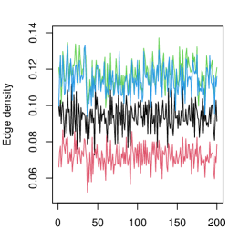
(a) $D_{t}$

(b) $D_{1,t}$

(c) $D_{0,t}$

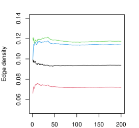
(d) $\bar{D}_{t}$

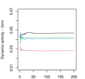
(e) $\bar{D}_{1,t}$

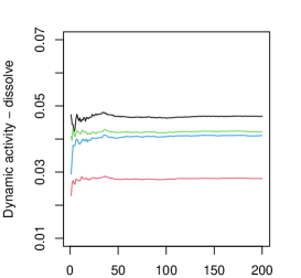
(f) $\bar{D}_{0,t}$

Figure S1: Time series plots of $\{D_{t}\}_{t=2}^{200}$, $\{D_{1,t}\}_{t=2}^{200}$, $\{D_{0,t}\}_{t=2}^{200}$, $\{\bar{D}_{t}\}_{t=2}^{200}$, $\{\bar{D}_{1,t}\}_{t=2}^{200}$ and $\{\bar{D}_{0,t}\}_{t=2}^{200}$ for the four simulated settings with $p=50$. The black, red, green and blue curves correspond to the settings $(\xi_{i},\eta_{i},a,b)=(0.7,0.8,30,15),$ $(0.6,0.7,20,20)$, $(0.6,0.7,15,10)$ and $(0.6,0.7,10,10)$, respectively.

C.2 A more general model

As stated towards the end of Section 3.3, a more general transitivity model admits the form:

$$\alpha_{i,j}^{t-1}(\boldsymbol{\theta})=\frac{\xi_{i}\xi_{j}e^{a_{1}U_{i,j}^{t-1}}}{1+e^{a_{1}U_{i,j}^{t-1}}+e^{b_{1}V_{i,j}^{t-1}}}\,,\qquad\beta_{i,j}^{t-1}(\boldsymbol{\theta})=\frac{\eta_{i}\eta_{j}e^{b_{2}V_{i,j}^{t-1}}}{1+e^{a_{2}U_{i,j}^{t-1}}+e^{b_{2}V_{i,j}^{t-1}}}\,,$$ (C.2)

with $\boldsymbol{\theta}=(a_{1},b_{1},a_{2},b_{2},\xi_{1},\ldots,\xi_{p},\eta_{1},\ldots,\eta_{p})^{{\scriptscriptstyle\top}}\in\mathbb{R}_{+}^{2p+4}>0$. Different from the transitivity model (3.3) introduced in Section 3.3, we allow $a_{1}\neq a_{2}$ and $b_{1}\neq b_{2}$ in (C.2). We adopt the same simulation settings as above, i.e. $(\xi_{i},a_{1},b_{1},\eta_{i},a_{2},b_{2})\in\{(0.7,30,15,0.8,30,15),$ $(0.6,20,20,0.7,20,20),$ $(0.6,15,10,0.7,15,10),$ $(0.6,10,10,0.7,10,10)\}$.

The two estimation methods are implemented in the same manner as in Section 5.2. Table S1 reports the resulting rMAEs over $400$ replications with $p=50$ and $n\in\{100,200,400\}$. The estimation for the parameters in $\alpha_{i,j}^{t-1}(\boldsymbol{\theta})$, namely $\xi_{i},a_{1}$ and $b_{1}$, exhibits the similar patterns as in Table 1, where $(\xi_{i},a_{1},b_{1},\eta_{i},a_{2},b_{2})=(0.7,30,15,0.8,30,15)$ achieves the best estimation accuracy. In contrast, the estimation for parameters in $\beta_{i,j}^{t-1}(\boldsymbol{\theta})$ deteriorates significantly, and especially for $a_{2}$ and $b_{2}$. Note that only some components of ${\bf X}_{t-1}$ with $X_{i,j}^{t-1}=1$, $t\in[n]\setminus[m]$ and $j\neq i$, were used in estimating parameters $a_{2}$ and $b_{2}$. For sparse networks, the total number of those data points is small. This is the intrinsic difficulty in estimating the parameters in $\beta_{i,j}^{t-1}(\boldsymbol{\theta})$. See also the relevant discussion at the end of Section 3.3.

Table S1: The means and STDs (in parenthesis) of rMAEs for estimating parameters in transitivity model (C.2) with 400 replications.

$(\xi_{i},a_{1},b_{1},\eta_{i},a_{2},b_{2})$		$n$		Estimation		$\alpha_{i,j}^{t-1}(\boldsymbol{\theta})$				$\beta_{i,j}^{t-1}(\boldsymbol{\theta})$
						$\xi_{i}$	$a_{1}$	$b_{1}$		$\eta_{i}$	$a_{2}$	$b_{2}$
(0.7, 30, 15, 0.8, 30, 15)		100		Initial		0.178 (0.026)	0.250 (0.023)	0.171 (0.005)		0.121 (0.019)	5.275 (8.602)	24.141 (24.917)
				Improved		0.103 (0.030)	0.117 (0.013)	0.066 (0.004)		0.112 (0.025)	5.687 (8.593)	26.259 (24.462)
		200		Initial		0.172 (0.022)	0.247 (0.021)	0.170 (0.004)		0.119 (0.023)	2.904 (6.050)	19.186 (22.146)
				Improved		0.093 (0.027)	0.113 (0.023)	0.064 (0.007)		0.111 (0.025)	3.356 (6.067)	21.646 (21.935)
		400		Initial		0.168 (0.016)	0.245 (0.019)	0.170 (0.004)		0.117 (0.021)	1.777 (3.273)	15.318 (18.832)
				Improved		0.088 (0.019)	0.109 (0.010)	0.063 (0.003)		0.109 (0.027)	2.180 (3.401)	17.636 (18.904)
(0.6, 20, 20, 0.7, 20, 20)		100		Initial		0.224 (0.004)	0.403 (0.023)	0.218 (0.005)		0.147 (0.007)	3.397 (8.745)	12.343 (19.473)
				Improved		0.138 (0.006)	0.135 (0.034)	0.081 (0.009)		0.130 (0.009)	3.585 (8.585)	13.754 (19.465)
		200		Initial		0.219 (0.002)	0.404 (0.017)	0.219 (0.003)		0.140 (0.008)	1.266 (3.404)	7.684 (11.048)
				Improved		0.123 (0.004)	0.124 (0.021)	0.079 (0.007)		0.122 (0.009)	1.479 (3.488)	9.146 (11.735)
		400		Initial		0.217 (0.002)	0.405 (0.012)	0.219 (0.002)		0.135 (0.008)	0.687 (0.316)	5.567 (8.182)
				Improved		0.114 (0.002)	0.117 (0.015)	0.075 (0.005)		0.117 (0.009)	0.787 (0.606)	6.830 (9.161)
(0.6, 15, 10, 0.7, 15, 10)		100		Initial		0.243 (0.003)	0.378 (0.015)	0.266 (0.005)		0.160 (0.019)	4.163 (10.012)	16.690 (24.226)
				Improved		0.136 (0.004)	0.178 (0.047)	0.098 (0.014)		0.146 (0.023)	4.322 (10.035)	18.638 (24.586)
		200		Initial		0.241 (0.002)	0.378 (0.011)	0.266 (0.004)		0.151 (0.019)	1.708 (4.439)	10.105 (17.250)
				Improved		0.124 (0.003)	0.162 (0.026)	0.090 (0.008)		0.138 (0.022)	1.785 (4.572)	11.984 (18.233)
		400		Initial		0.240 (0.001)	0.379 (0.008)	0.266 (0.003)		0.146 (0.018)	1.312 (3.015)	7.461 (14.351)
				Improved		0.117 (0.002)	0.159 (0.018)	0.088 (0.005)		0.133 (0.022)	1.202 (3.158)	9.039 (15.240)
(0.6, 10, 10, 0.7, 10, 10)		100		Initial		0.242 (0.003)	0.534 (0.026)	0.279 (0.005)		0.165 (0.020)	10.003 (20.550)	25.992 (28.225)
				Improved		0.136 (0.005)	0.254 (0.073)	0.101 (0.013)		0.152 (0.025)	10.210 (20.584)	28.117 (28.413)
		200		Initial		0.240 (0.002)	0.536 (0.019)	0.279 (0.004)		0.162 (0.022)	5.987 (15.780)	21.763 (26.073)
				Improved		0.125 (0.003)	0.238 (0.045)	0.095 (0.007)		0.149 (0.027)	6.113 (15.673)	24.344 (26.729)
		400		Initial		0.239 (0.001)	0.535 (0.013)	0.279 (0.003)		0.157 (0.023)	2.956 (6.909)	16.885 (21.903)
				Improved		0.117 (0.002)	0.231 (0.028)	0.094 (0.005)		0.144 (0.028)	2.817 (7.196)	19.332 (23.305)

Appendix D Conference interactions

We apply our model to an additional dynamic network dataset, in this case of face-to-face interactions among attendees of an academic conference. The conference in question was the 2009 congress of the Société Française d’Hygiène Hospitalière (SFHH) (Cattuto et al., 2010; Génois and Barrat, 2018). The original data was collected automatically by RFID badges worn by the conference participants. We analyze a subset of the data corresponding to an active portion of the first day of the congress (June 4, 2009) from about 11:00AM to 6:00PM among the $p=200$ most active participants out of the total 403. Each of the $n=22$ network snapshots corresponds to a non-overlapping time window, with $X_{i,j}^{t}=1$ if participants were in close proximity at any time during the prior 20 minutes.

Similar to Section 6, we summarize some key features of this dataset. Figure S2 (left panel) shows that while there are some spikes in edge density, there is no clear increasing or decreasing pattern, so we choose to model this dataset with a single AR network model. Figures S2 and S3 show empirical evidence of temporal edge dependence, as well as transitivity effects: after accounting for edge density, edges persist at a higher rate than they grow, they more often grow for node pairs which had more common neighbours, and they more often dissolve for node pairs which had more disjoint neighbours.

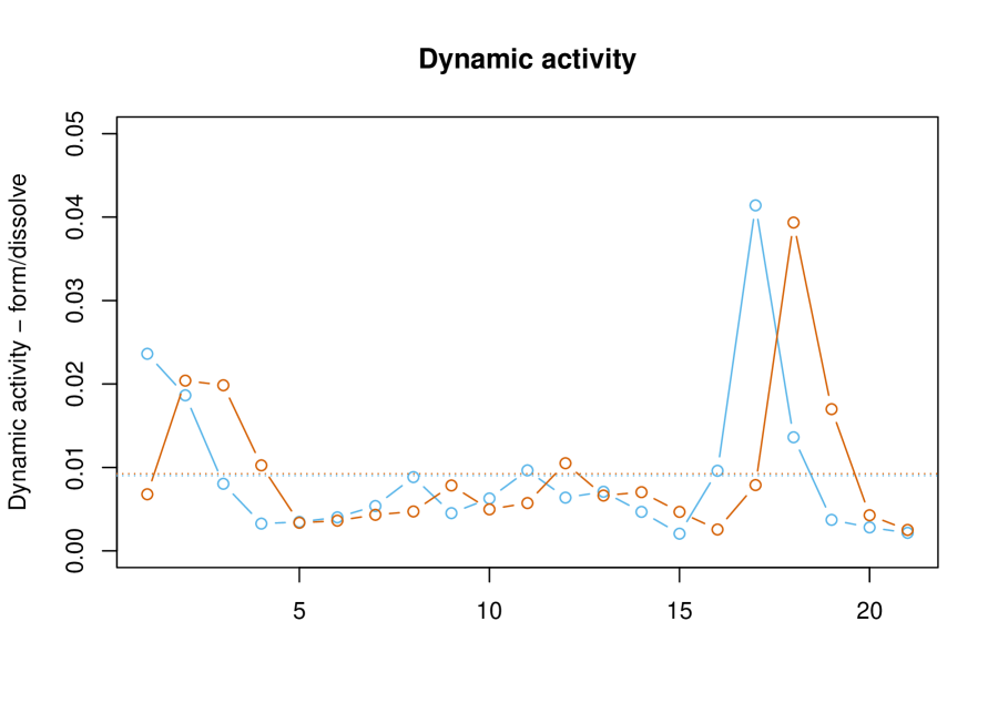
Figure S2: Evolution of edge density (left panel), percentage of grown (blue) and dissolved (orange) edges (right panel), SFHH participant networks.

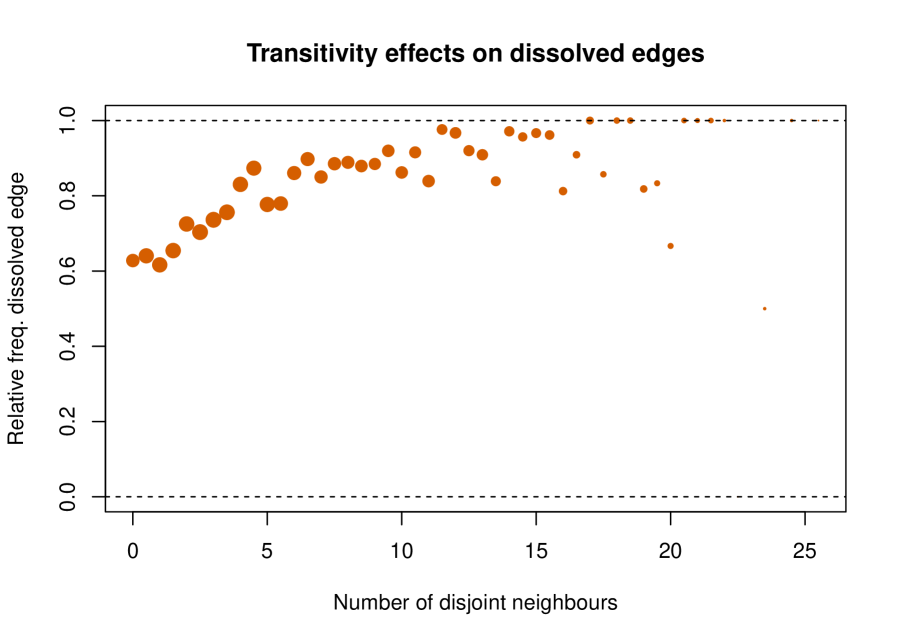
Figure S3: Left panel: relative edge frequencies, $\{\mathcal{U}_{c}\}_{c\geq 0}$. Right panel: relative non-edge frequencies, $\{\mathcal{V}_{c}\}_{c\geq 0}$. In both panels, point size is proportional to log of sample size.

Fitting our AR network model with transitivity, we estimate $\hat{a}=26.75$ and $\hat{b}=15.14$, confirming these empirical dynamic effects of common and disjoint neighbours. We summarize the estimates of the local parameters $\{\xi_{i}\}_{i=1}^{200}$ and $\{\eta_{i}\}_{i=1}^{200}$ in Figure S4.

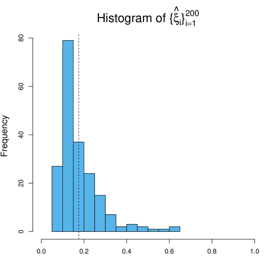
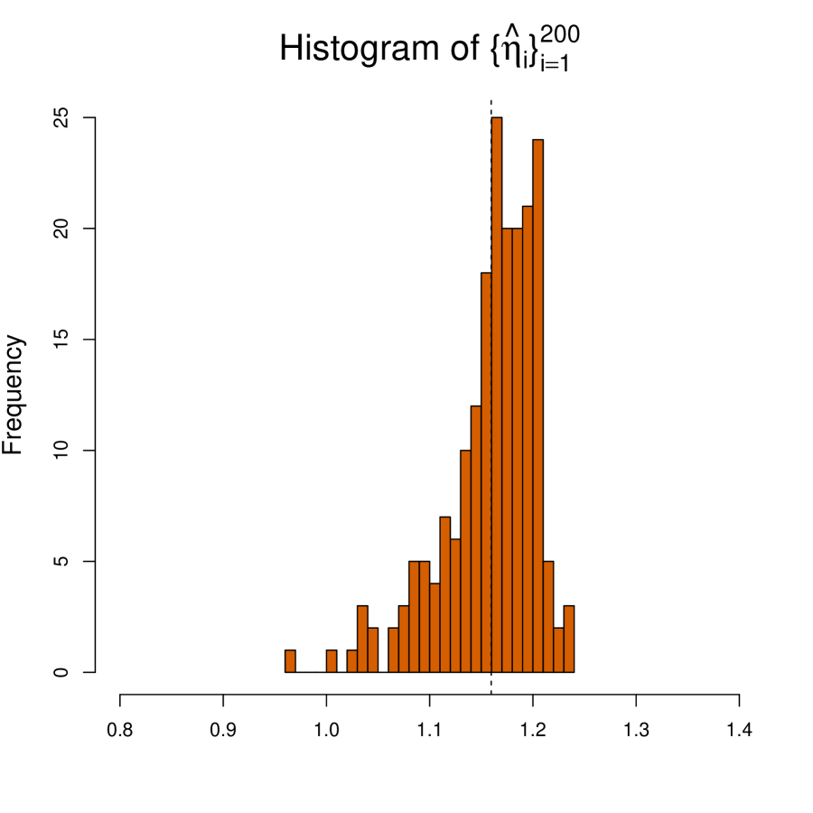
Figure S4: Histograms and scatter plot of estimates $\{\hat{\xi}_{i}\}_{i=1}^{200}$ and $\{\hat{\eta}_{i}\}_{i=1}^{200}$.

The estimates $\{\hat{\xi}_{i}\}_{i=1}^{200}$ have mean 0.18 and a longer right tail, while the estimates $\{\hat{\eta}_{i}\}_{i=1}^{200}$ have mean 1.16 and a longer left tail. Moreover, their scatter plot shows that there is a negative relationship between these estimates for a given node. All of these observations are consistent with overall degree heterogeneity of the network. The estimates $\{\hat{\xi}_{i}\}_{i=1}^{200}$ have a wide range from 0.05 to 0.64, while the estimates $\{\hat{\eta}_{i}\}_{i=1}^{200}$ are all between 0.97 and 1.24. This implies that conference attendees are more heterogeneous in their propensity to form new connections, than in their propensity to extend the length of existing ones.

Model	AIC	BIC
Transitivity AR model	48013	52412
Global AR model	48037	48059
Edgewise AR model	109284	544815
Edgewise mean model	71205	288970
Degree parameter mean model	54061	56250

Table S2: AIC and BIC performance for conference interaction data

Finally, we compare our model to the same competing models described in Section 6 in terms of AIC and BIC. These results are reported in Table S2. Our AR network model with transitivity achieves the smallest AIC, followed closely by the global AR model, which only has 2 parameters. The global AR model achieves the smallest BIC, thus in both cases the best model incorporates temporal edge dependence. Under either criterion, the two edgewise models require $O(p^{2})$ parameters and thus perform poorly, as there are relatively many nodes ($p=200$) compared to network samples ($n=22$). Although the transitivity model has $O(p)$ parameters, it achieves the smallest AIC and the 2nd smallest BIC, suggesting that degree heterogeneity parameters and the imposed transitivity form are an effective parameterization to summarize the structure in this dataset.

References

• (1)
• Athreya et al. (2017) Athreya, A., Fishkind, D. E., Tang, M., Priebe, C. E., Park, Y., Vogelstein, J. T., Levin, K., Lyzinski, V., Qin, Y. and Sussman, D. L. (2017). Statistical inference on random dot product graphs: a survey, Journal of Machine Learning Research (JMLR) 18: Paper No. 226, 92.
• Azuma (1967) Azuma, K. (1967). Weighted sums of certain dependent random variables, The Tohoku Mathematical Journal. Second Series 19: 357–367.
• Brémaud (1998) Brémaud, P. (1998). Markov Chains: Gibbs Fields, Monte Carlo Simulation, and Queues, Springer.
• Cattuto et al. (2010) Cattuto, C., Van den Broeck, W., Barrat, A., Colizza, V., Pinton, J.-F. and Vespignani, A. (2010). Dynamics of person-to-person interactions from distributed RFID sensor networks, PloS one 5(7): e11596.
• Chang et al. (2021) Chang, J., Chen, S. X., Tang, C. Y. and Wu, T. (2021). High-dimensional empirical likelihood inference, Biometrika 108(1): 127–147.
• Chang et al. (2023) Chang, J., Shi, Z. and Zhang, J. (2023). Culling the herd of moments with penalized empirical likelihood, Journal of Business & Economic Statistics 41(3): 791–805.
• Durante and Dunson (2016) Durante, D. and Dunson, D. B. (2016). Locally adaptive dynamic networks, The Annals of Applied Statistics 10(4): 2203–2232.
• Friel et al. (2016) Friel, N., Rastelli, R., Wyse, J. and Raftery, A. (2016). Interlocking directorates in irish companies using a latent space model for bipartite networks, Proceedings of the national academy of sciences 113(24): 6629–6634.
• Génois and Barrat (2018) Génois, M. and Barrat, A. (2018). Can co-location be used as a proxy for face-to-face contacts?, EPJ Data Science 7(1): 1–18.
• Graham (2016) Graham, B. (2016). Homophily and transitivity in dynamic network formation, London: Institute for Fiscal Studies .
• Hall and Heyde (1980) Hall, P. and Heyde, C. C. (1980). Martingale limit theory and its application, Probability and Mathematical Statistics, Academic Press, Inc. [Harcourt Brace Jovanovich, Publishers], New York-London.
• Hanneke et al. (2010) Hanneke, S., Fu, W. and Xing, E. (2010). Discrete temporal models of social networks, Electronic Journal of Statistics 4: 585–605.
• Jiang et al. (2023a) Jiang, B., Leng, C., Yan, T., Yao, Q. and Yu, X. (2023a). A two-way heterogeneity model for dynamic networks, arXiv:2305.12643 .
• Jiang et al. (2023b) Jiang, B., Li, J. and Yao, Q. (2023b). Autoregressive networks, Journal of Machine Learning Research 24(227): 1–69.