Quantum metrology of rotations with mixed spin states
Abstract
The efficiency of a quantum metrology protocol can be considerably reduced by the interaction of a quantum system with its environment, resulting in a loss of purity and, consequently, a mixed state for the probing system. In this paper we examine the potential of mixed spin- states to achieve sensitivity comparable, and even equal, to that of pure states in the measurement of infinitesimal rotations about arbitrary axes. We introduce the concept of mixed optimal quantum rotosensors based on a maximization of the Fisher quantum information and show that it is related to the notion of anticoherence of spin states and its generalization to subspaces. We present several examples of anticoherent subspaces and their associated mixed optimal quantum rotosensors. We also show that the latter maximize negativity for specific bipartitions, reaching the same maximum value as pure states. These results elucidate the interplay between quantum metrology of rotations, anticoherence and entanglement in the framework of mixed spin states.
I Introduction
The development of modern measurement techniques is closely tied to advances in all fields of science. The unprecedented manipulation and control of quantum systems is now opening up opportunities for quantum-enhanced metrology, which has become a major field of study. A fundamental example is the precise detection of rotation, first developed for inertial navigation and now used to detect minute magnetic fields through the spin of particles. The study of the measurement of a rotation using a quantum system as a probe reveals the existence of certain states where the estimate can be improved by quantum effects [1, 2, 3]. The main tool for estimating the sensitivity of the state of a quantum system is the quantum Cramér-Rao bound (QCRB) [4, 5]. If we have no a priori knowledge of the direction of the axis of rotation, we need to find a quantum state that is very sensitive whatever the axis. This corresponds exactly to the notion of an optimal quantum rotosensor (OQR), which has been extensively studied for pure spin- states in recent years [6, 7, 8, 9, 10, 11]. In particular, it was discovered that the OQRs for infinitesimal rotations are anticoherent (AC), a property of quantum states first introduced by Zimba [12] and studied in many works, see e.g. [13, 14, 15, 16, 17, 18, 19, 20]. An anticoherent state is characterised by the expectation values of the first moments of the angular momentum being homogeneous, i.e. with no preferred direction [12, 13]. In this sense, they are the opposite of spin-coherent states [21, 12].
Under real conditions, a quantum system interacts with its environment and its state becomes mixed, i.e. a statistical mixture of pure states. In this scenario, it is not clear that the conditions required for a mixed state to be an OQR are the same as those defining pure OQRs. While the characterization of the most sensitive mixed states with a fixed spectrum for an infinitesimal rotation over a known axis, and in general for an infinitesimal transformation given by any generator of the Lie algebra, has been solved in Ref. [22], it remains open for an unknown axis. Additionally, the authors of Ref. [23] have characterized the mixed states with the best metrological power via the purification of the state. In this work, precisely, we derive conditions for obtaining the ultimate detection sensitivity of an infinitesimal rotation about an unknown axis with mixed states. We show how to write these conditions in terms of anticoherent subspaces, defined as vector spaces of anticoherent states, which were first introduced and studied by Pereira and Paul-Paddock [24]. It turns out that these AC subspaces also have applications in a holonomic quantum computation approach resilient to rotational noise [25].
Multipartite entanglement is a resource to achieve the ultimate sensitivity of measurement with quantum states [26, 3, 27, 28, 29, 30, 31, 32], also known as the Heisenberg limit. For pure states, a faithful measure of bipartite entanglement [33, 34] with respect to a bipartition of the system is given by the entanglement negativity [35, 33]. For mixed states, the negativity is only a witness of entanglement, except for qubit-qubit and qubit-qutrit systems [36, 37]. Negativity is easy to compute and is at the core of the notion of distillable entanglement [38, 39]. Therefore, in this work we have chosen to study the entanglement of mixed OQRs based on this quantity.
For an individual spin--system, the notion of entanglement has no obvious meaning. It is only by interpreting spin- states as symmetric -qubit states that the notion becomes relevant and meaningful. In this correspondence, the quantum property of anticoherence is related to negativity since pure AC states maximise negativity for a certain bipartition of the -qubit Hilbert space [20]. In this paper, we also study the possible connections between negativity and anticoherence for mixed states.
The paper is organized as follows: After reviewing the basic concepts in Sec. II, we derive the conditions for pure and mixed states to be OQR in Sec. III. We study the question of the existence of mixed OQRs for small spin and present illustrative examples in Secs. IV–V, respectively. The discussion concerning the negativity of mixed OQR states is presented in Sec. VI. Finally, we summarize our results in Sec. VII.
II Concepts and mathematical framework
II.1 Fidelity and Quantum Fisher Information for pure and mixed states
Let us consider a general quantum state in a Hilbert space where the elements of the rotation group are represented by , where and are the axis-angle parameters, and is an angular momentum operator. The Hilbert space has a unique decomposition into subspaces that transform independently by a transformation (the double cover of ) through one of its irreducible representations (irreps), labeled by
| (1) |
where the superindex of each subspace indicates the -dimensional irrep (spin ). For simplicity, we restrict our search to states living in a single subspace , later interpreted as the symmetric sector of the Hilbert space of qubits. As we explain in the next subsection, the sensitivity of a state to detect infinitesimal rotations increases with a factor proportional to , suggesting that it is convenient to work with states belonging to the subspace associated with the the highest-dimensional irrep. A similar result has been proved for symmetric multiqudit pure-states [40]. The fidelity between a state and its image under the rotation reads
| (2) |
Our main goal is to find the states that minimize averaged over all possible axes of rotation
| (3) |
for an infinitesimal angle of rotation . For mixed states in the Hilbert-Schmidt space of operators , we use the Uhlmann-Jozsa fidelity [41, 42], which can be related to the Bures distance [4],
| (4) |
Like any well-defined fidelity function for mixed states [43], the Uhlmann-Jozsa fidelity coincides with the fidelity (2) when the states are pure. For infinitesimal angles about an axis of rotation , one must calculate the Quantum Fisher information (QFI) , given by the Bures distance between and the infinitesimally close state , which reads [4]
| (5) |
II.2 Multipole operators
The multipole (or polarization) operators , with and [44, 45, 46], form an orthonormal basis with respect to the Hilbert-Schmidt inner product . Hence, a mixed state expanded in this basis reads
| (6) |
where and is the maximally mixed state in . Since [45], the hermiticity of the density matrix enforces that . Additionally, the ’s are traceless operators except for . The multipole operators can be constructed as products of the angular momentum operators and (see e.g. Eq. (4), p. 44 of Ref. [45]). For example,
| (7) | ||||
More details on multipole operators can be found in Refs. [44, 45, 46].
II.3 Anticoherent states and subspaces
We begin with the definition of anticoherent states as given in Ref. [12], extended here to mixed states.
Definition.
A state , either pure or mixed, is -anticoherent if is independent of for , where . For the sake of brevity in this paper, we will use the abbreviation -AC for -anticoherent.
The condition of -anticoherence is equivalent to a zero expectation value of the multipole operators, i.e. , for and [13]. In particular, the 1-anticoherence condition for pure states reduces to for [16]. The -anticoherence of a state can be quantified with the functions 111The functions (8) define measures of anticoherence for pure states, see Ref. [16] for more details.
| (8) |
for integer , where is the reduced density matrix obtained after tracing out spin-1/2 among the making up the spin. These functions range from for spin-coherent states to for -AC states [16]. In addition, a state is -AC if and only if for [13]. By definition, -anticoherence implies -anticoherence for . While for pure states there are no -AC states for certain values of [16], one can always find, at least sufficiently close to the maximally mixed state, states which are AC to any order . We give a proof of the last statement in Appendix A.
The notion of an anticoherent state was generalized in Ref. [24] to subspaces as follows.
Definition.
A -dimensional subspace of is -AC if any state is -AC. Such a subspace will be referred to as AC subspace.
A necessary, but not sufficient, condition for a basis to span a -AC subspace is that its vectors are -AC states. Orthonormal bases made of -AC states for the whole Hilbert space have been studied in Ref. [17].
There are equivalent characterizations for AC subspaces as specified in the following lemma.
Lemma 1
Let be a subspace of dimension of . The following statements are equivalent:
-
1.
is a AC subspace.
-
2.
A (non-necessarily orthogonal) basis of satisfies the following conditions:
(9) for any , and .
-
3.
Any pair of states satisfies the following conditions:
(10) for any and .
In particular, a AC subspace fulfills
| (11) |
for any pair of states and (note that is not excluded). One method of searching for AC subspaces, which is well suited to numerical approaches, is to define an objective function which takes as arguments vectors and which is zero if and only if these vectors span a AC subspace for certain values of . To this end, we first introduce, for integers , the functions
| (12) |
where is now assumed to be an orthonormal basis of some subspace of dimension . The last equation can be re-written as
| (13) |
with
| (14) |
The positive function is zero if and only if all the terms in the sum (12), which are all positive, vanish simultaneously. Therefore, the objective function
| (15) |
is zero if and only if for any and and any , which corresponds to the second equivalent statement of a subspace being a AC subspace mentioned in Lemma 1. In this work, most of the AC subspaces presented in Sections IV-V were found by searching for zeros of the objective function by numerical optimization.
II.4 Negativity of pure AC states
The negativity of a state of a bipartite system with Hilbert space is defined as [35, 33]
| (16) |
| (17) |
with an orthonormal basis of , and an orthonormal subset of . An immediate consequence of (17) is that of a pure -AC state is maximal and equal to [20]
| (18) |
This result is no longer valid for mixed states, as shown by the example of the maximally mixed state , which is -AC to any order but for which because is fully separable. Consequently, for arbitrary mixed states, there is a priori no relationship between negativity and anticoherence. However, in Sec. VI, we will uncover a connection between -AC subspaces and mixed states with maximal negativity over certain bipartitions.
III Optimal quantum rotosensors for infinitesimal rotations
Now, let us consider the problem of optimal quantum rotosensors (OQR) [6, 7, 9, 10] for infinitesimal rotations, i.e. for rotation angles . The best possible estimate of , i.e., the minimum variance of the estimator of the parameter , is given by the QCRB [4, 48, 22], , which is written here in terms of the QFI (5) and achievable by optimizing over all Positive Operator Valued Measures. Here, is the number of times the measurement is repeated. As the axis of rotation is unknown, we seek to minimize the QCRB averaged over all rotation axes
| (19) |
The r.h.s. of the inequality is lower bounded by Jensen’s inequality [49]
| (20) |
which is tight when the function is independent of the variable of integration . Therefore, our goal is to find a state that minimizes and saturates the QCRB, which is the case when satisfies the following two conditions:
| (21) | |||
| (22) |
As we will show in the following, these two conditions lead naturally to the notion of AC states and subspaces.
III.1 Pure states
For a pure state , the Uhlmann-Jozsa fidelity (4) reduces to (2), and the QFI (5) is just the variance of the angular momentum component along the direction
| (23) |
The averaged QFI in all directions is then equal to
| (24) |
where we used the identity
| (25) |
to evaluate the integral defining the average. The conditions (21)–(22) for a pure state are fulfilled whenever and for any , that is when is a 2-AC state [8]. In this case, the optimal lower bound for the averaged QCRB reads
| (26) |
that is inversely proportional to . This means that the higher the spin quantum number, the better the optimal estimate that can be obtained.
| Pure states | Mixed states | |
|---|---|---|
| Condition (21): | is 1-AC | is a 1-AC subspace |
| Condition (22): | is 2-AC | is 2-AC |
III.2 Mixed states
Now, we consider mixed states of a spin-, . Let denote the eigenvalues and the corresponding eigenvectors of with the dimension of . Without loss of generality, we label by the eigenvectors with the non-zero eigenvalues, which span the image of , with . When the state is not full rank (), the states with span the kernel of , . Both and are complementary subspaces in . We denote by and the projectors onto and , respectively,
| (27) |
The QFI (5), in terms of the Uhlmann-Jozsa fidelity (4), is now given for an infinitesimal rotation about the axis by [4, 48, 22]
| (28) |
with
| (29) |
We now rewrite Eq. (28) as follows
| (30) | ||||
It is easy to observe from the last equation that Eq. (28) reduces to Eq. (23) for the case of pure states. The QFI for mixed state (30) averaged over all directions is then given by
| (31) |
Hence, the first condition (21) defining a mixed OQR reduces to satisfying for and any pair of states in , which is equivalent to being a 1-AC subspace. This condition implies that is a 1-AC state, but it is stronger. Once the first condition (21) is met, the second condition (22) reduces to being independent of , i.e., being a 2-AC state. Remarkably, the mixed states satisfying these two conditions, which we now call mixed OQRs, are as good estimators as the pure OQRs because they give the same lower bound on the averaged QCRB (26). We can therefore conclude that a less pure spin state is not necessarily a worse estimator.
We summarize the conditions we have found for a state to be OQR in Table 1, both for the pure case and for the mixed case. The condition (22) can always be fulfilled for any value of the spin quantum number by sufficiently mixing a state with the maximally mixed state and thus decreasing its purity (see proof in Appendix A). On the other hand, the first condition is all the more difficult to fulfill the higher the rank of the state is. There is therefore a certain tension between the two conditions. Since is of dimension equal to the rank of , condition (21) will be harder to meet for highly mixed states. The rank of a state is in fact directly related to the minimal purity it can reach, since . For a given spin quantum number , the maximum dimension of a 1-AC subspace sets in turn a lower bound on the purity attainable by mixed OQRs. We have determined the value of by numerically searching for zeros of the objective function (15) for (see discussion in Sec. V and Fig. 2, where we show the dependence of on ).
A general approach to identify mixed OQRs, which we will pursue in the next section, is as follows. The first step is to find 1-AC subspaces which can be used to construct mixed states satisfying the condition (21), followed by the search for an appropriate mixture of states within that will satisfy the condition (22). Another, more direct approach is to find 2-AC subspaces from which a mixture of basis states will automatically define a mixed OQR. In both cases, it is essential to search for and identify AC subspaces.
IV Mixed OQRs for small spin
While pure spin states defining OQRs have been extensively studied in the literature [7, 9, 10], we present here several examples of mixed OQRs, first performing a systematic search for small spin quantum numbers.
IV.1 Spin 1
The only 1-AC spin-1 states are given by [14], where is the rotation matrix in the -irrep parametrized with the Euler angles. First, let us search for a AC subspace spanned by an orthonormal basis . The two states must be obtained from the state by rotations, since they must be 1-AC. Moreover, since the order of anticoherence is independent of the orientation of the subspace, we can reorient the basis so that
| (32) | ||||
where the vectors indicate the components of the states in the basis, with . By direct calculation, we obtain and , which cannot be made simultaneously zero. Consequently, there are no AC subspaces with . On the other hand, the only 2-AC state of spin-1 is the maximally mixed state . Therefore, no state, pure or mixed, of a spin can be an OQR.
IV.2 Spin 3/2
As for spin 1, there is only one 1-AC state, up to rotation, given by the GHZ state [14]. We can start searching for a AC subspace spanned by a reoriented orthonormal basis such that
| (33) |
The orthogonality condition has three solutions: 1) and , 2) and , and 3) and for some integer numbers and . The three solutions have the same expression for some complex numbers with . By direct calculation, we get that and we can conclude that there are no AC subspaces, and thus no mixed OQRs.
In order to study the effect on the QCRB of a deviation from the condition (21) while satisfying the condition (22), let us consider a family of 2-AC mixed spin-3/2 states in the purity range , as derived in Appendix B. In particular, we show there that the 2-AC mixed state with the largest purity is the rank-two state with
| (34) |
As we have already shown above, none of these 2-AC states have an image spanning a 1-AC subspace.
Despite the absence of OQRs, we can compare the respective QCRBs (19) reached by mixed and pure states. In particular, we have that
| (35) |
meaning that the pure GHZ state is only slightly better than the 2-AC mixed state with purity .
IV.3 Spin 2
This is the smallest spin quantum number for which there is a two-dimensional 1-AC subspace. Such a subspace is spanned by the orthogonal pure states
| (36) |
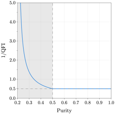
Since both states are 2-AC [15, 16], so is any mixture , which therefore defines a mixed OQR. By varying the eigenvalues of through , we can obtain mixed OQRs with purity . We prove in Appendix C that the AC subspace spanned by the states (36) is unique up to a rotation. As a result, mixed OQRs are all of the above form. For mixed states of higher rank and smaller purity, the QCRB increases as the purity decreases. We can confirm this trend by considering the uniparametric family of mixed states
| (37) |
where the states are given in Eq. (36). For , is an OQR, but not for . The purity of increases monotonically with as
| (38) |
We also find that the QFI for is independent of and its inverse is equal to
| (39) |
In Fig. 1, we plot as a function of . We can see that, for , the inverse of the QFI starts to increase until infinity is reached for the maximally mixed state (). Therefore, the QCRB increases (and thus the metrological power of the state decreases) as the purity decreases and is below , as announced above.
V Illustrative examples of AC subspaces and mixed OQRs
We now present several examples of AC subspaces found numerically by using the objective function (15) and, subsequently, explore the possibility to get a mixed OQR.
V.1 1-AC subspaces
V.1.1 AC subspaces
There are several AC subspaces. A first example is the space spanned by the states
| (40) | ||||
The candidates for mixed OQRs are given by a mixture of a generic basis of , , with
| (41) | ||||
The function for this family reads
| (42) |
with maximum achieved for and any values, or for and any weights and phase . We can see that these mixed states are almost 2-AC, but do not fulfill condition (22). Hence, they are not a mixed OQR.
A second example of a AC subspace is the vector space spanned by the states
| (43) | ||||
with , and . Again, we search for a 2-AC mixed state given by a mixture of a generic basis of the AC subspace . We get that the maximum of is equal to
| (44) |
achieved for the equally weighted mixture for any basis of . Once again, the corresponding mixed state is not 2-AC, so is not a mixed OQR.
V.1.2 AC subspace
The first 3-dimensional 1-AC subspace emerges for , and is spanned by the states
| (45) | ||||
The measure of 2-anticoherence of a general coherent superposition , with and , is given by
| (46) |
The maximum of in Eq. (46) under the normalization constraint is equal to 222The maximum is achieved e.g. for and .. Hence, no pure state is 2-AC. On the other hand, the statistical mixture of the states (45) with weights yields a with . This then shows that for , is 2-AC and therefore a mixed OQR. This OQR, explicitely given by
| (47) |
is the first example of a mixed OQR without any pure OQR in its image .
V.2 2-AC subspaces
The AC subspaces are particularly interesting because any convex combination of any orthonormal basis of yields a mixed OQR. In this subsection, we give some examples of 2-AC subspaces for small values.
V.2.1 AC subspace
The first instance of a 2-AC subspace is found for . An example is the space spanned by the states
| (48) | ||||
V.2.2 AC subspace
For spins larger than , we did not numerically find other AC subspaces up to the value . One example is spanned by the states
| (49) | ||||
V.3 AC subspaces of arbitrary dimension
Previously, we used the 1- and 2-AC subspaces to create families of mixed OQRs. Here, we take a different approach and show that one can find AC subspaces of order and of any dimension with sufficiently large spin using techniques similar to those outlined in Ref. [15]. For a spin- system with a half-integer number, the subspace spanned by the vectors
| (50) |
with is a AC subspace. Here, is a string of zeroes in the vector, with the convention that means we do not add any extra zeroes. In the case where is an integer and , we can add the following extra state to increase the dimension of the 1-AC subspace
| (51) |
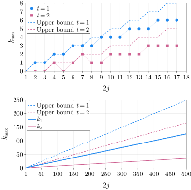
The dimension of these generic 1-AC subspaces, denoted by , is given by
| (52) |
and grows linearly as (see e.g. Fig. 2). As an illustration, we write the vectors spanning the AC subspaces for in Table 2. The zeroes in the states components ensure that for any pair of states, where we used Eq. (7). On the other hand, because with for .
| Spin | Basis of the AC subspace |
|---|---|
| 5 | |
| 11 | |
| 35/2 |
In the same way, it is possible to construct a generic AC subspace for of dimension
| (53) |
with
| (54) |
spanned by the states
| (55) |
with . Again, the zeroes in the states components guarantee that for every , any , and any pair of states . This because the respective with contain one or two ladder operators (7). In addition, the zeroes of the state components guarantee that for different states. On the other hand, , with , is fulfilled by the property that the coefficients and are associated with eigenstates whose magnetic quantum number is opposite. Finally, it is possible to satisfy the equality , where by choosing the parameters and , which we can considered as positive real numbers, such that (normalization of the state) and
| (56) |
Indeed, the above equation always has a solution for the value of defined in Eq. (54). The dimension of the AC subspace (55) grows asymptotically as . Some examples of AC subspaces constructed using this approach are given in Table 3.
In Fig. 2 we show the dimension of the 1- and 2-AC subspaces given by our construction as a function of the spin quantum number . We note that both grow slowly but linearly in the asymptotic limit . We also plot the largest dimension of a AC subspace found numerically for and . The value for 1-AC subspaces puts a lower bound on the purity of optimal OQRs, . Our numerical results show that the Corollary 2 in Ref. [24], stating that the largest 1-AC subspace of spin states has dimension , is not tight.
VI Negativity and anticoherent subspaces
The quantum improvement in metrological power is generally attributed to entanglement. To find out if this is the case for mixed OQRs, we discuss in this section the relationship between the negativity of mixed states constructed from -AC subspaces, particularly when they define mixed OQRs. Despite the classical character of a mixture of states, we will show that a mixed state such that is a AC subspace maximizes all the negativities for . In particular, the negativity of these mixed states with respect to the bipartitions with is equal to that of the most entangled pure states (18). Because of the relevance of this result, we express it as a theorem whose proof is provided in Appendix D:
Theorem 1
Let be a mixed state such that is a AC subspace. Then , seen as a -qubit symmetric state, maximizes the negativity with respect to the bipartition with .
An important consequence of (the proof of) Theorem 1 is an upper bound on the dimension of AC subspaces, given by
| (57) |
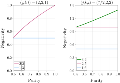
In particular, for 1-AC subspaces, it gives a more strict bound than the one given in Corollary 2 of Ref. [24]. We plot this upper bound in Fig. 2. On the other hand, we plot the negativity for some AC subspaces presented in the previous section in Fig. 3. We can observe the constant value of the negativity for the bipartitions associated to the anticoherence order of the AC subspaces but not for the others which decrease when the purity decreases. In summary, mixed OQRs, which come from 1-AC subspaces, are maximally entangled states with respect to the negativity for the bipartition , despite their variable purity.
VII Conclusions
In this work, we established the necessary conditions, as outlined in Table 1, for a mixed spin- state to achieve optimal sensing capabilities for infinitesimal rotations about arbitrary axes, as dictated by the QCRB averaged over all rotation axes (19). While pure states are OQRs when they are 2-AC, the mixed scenario adds the additional condition that must be a 1-AC subspace (see Eq. (21)), introducing the need for anticoherent subspaces to achieve the optimal sensitivity in the measurement of rotations. As a result, we studied the existence of -AC subspaces and, in particular, the maximum dimension that 1-AC subspaces can have for a given value of (see Fig. 2). This value is important because we have shown that it sets a lower bound on the purity of mixed OQRs. Our detailed study of mixed OQRs for small spin quantum numbers shows that the first mixed OQR is found for spin (see Eq. (36)). Furthermore, we presented various examples of AC subspaces and mixed OQRs, including 2-AC subspaces that generate a continuous family of mixed OQRs, and cases where the mixed OQRs arise from a mixture of non-OQR pure states (see Eq. (47)). We showed how to construct 1- and 2-AC subspaces of any dimension for sufficiently high spin by providing explicit subspaces bases (see Tables 2–3 for selected examples). For these subspaces, we showed that the dimension increases linearly with the spin quantum number , and we have compared it to the maximum dimension obtained numerically for the same spin (see Fig. 2). Additionally, we provided an upper bound on (Eq. (57)) in terms of the spin and the anticoherence order . One of the main conclusions of our work is that mixed states can achieve the same sensitivity as optimal pure states. This property can be related to entanglement by interpreting spin states as symmetric multiqubit states. More precisely, our Theorem 1 establishes that any state obtained by mixing pure states from a -AC subspace, in particular mixed OQRs, maximizes all negativities for the bipartitions with . Therefore, mixed spin- OQRs not only have genuine multipartite entanglement, as was already known to be necessary for pure states to be OQRs [29, 30, 31], but they are also maximally entangled states with respect to the negativity for the bipartition among all symmetric states.
Acknowledgments
ESE acknowledges support from the postdoctoral fellowship of the IPD-STEMA program of the University of Liège (Belgium). JM acknowledges the FWO and the F.R.S.-FNRS for their funding as part of the Excellence of Science programme (EOS project 40007526). CC would like to acknowledge partial financial support from the DGAPA-UNAM project IN112224.
Appendix A Existence of anticoherent mixed states to any order
In this Appendix, we prove the existence of mixed AC states of any order other than the maximally mixed state. More generally, we prove the existence of mixed states with for any subset of indices and . We start with the maximally mixed state and a mixture
| (58) |
with an operator such that
| (59) |
with arbitrary coefficients making Hermitian. The state is Hermitian, with trace , and positive for a sufficiently small . In fact, if we denote the lowest (and therefore potentially negative) eigenvalue of , then is a valid state for . In particular, if we consider , the state defined above is -AC.
Appendix B 2-AC spin-3/2 mixed states
Here, we characterize the set of -AC spin-3/2 mixed states. By definition, they have an expansion in the multipole operator basis of the form
| (60) |
We can reduce the number of variables by a global rotation rendering and . Moreover, by the hermiticity of the state, we also get and . We now perform the change of variables
| (61) | ||||
so that
| (62) | ||||
with and where all the new variables are real. Finally, must be a valid state, i.e., its eigenvalues
| (63) |
must be positive, where
| (64) | ||||
The positivity of is guaranteed if the lowest eigenvalue is positive, which is fulfilled for . In particular, if we are interested in the -AC state with the highest purity , we must maximize the variable for valid states, i.e., for states with . To fulfill this, we minimize the factor of the variable in , , achieved for . The minimum is given by and the corresponding state has doubly-degenerated eigenvalues . Then, we can take , leading to the state
| (65) |
with eigenvectors (34) and purity .
Appendix C Uniqueness of the AC subspace
Here, we prove that, up to a rotation, the AC subspace spanned by the states (36) is unique. We begin by considering a generic AC subspace with basis . By definition, the states are 1-AC. We then rotate the subspace to , now with basis , such that has the form of a generic spin-2 1-AC state (as given in Ref. [15])
| (66) |
where . The unnormalized vectors for read
| (67) | ||||
We can see that for , the set
| (68) |
consists of 4 orthogonal vectors. Its orthogonal complement has dimension 1 and, by direct calculation, consists of the state
| (69) |
The latter state must be equal to because is 1-AC subspace and must obey the condition (11). The explicit expressions of the states show that is the same subspace spanned by the states (36) whatever the value of . In the special case , it is shown in Ref. [15] that these states are, up to a rotation, equal to the state . We can then study this case by starting with . Generating the set in the same way, which now contains 3 vectors, we obtain that must have the form
| (70) |
with . However, since must be 1-AC, we must have that . Consequently, is spanned by the states
| (71) |
which, after a rotation by about the axis, is equivalent to the subspace spanned by the states
| (72) |
Again, this AC subspace is equivalent to the subspace spanned by the states (36).
Appendix D Maximal negativity of mixed states
Before proving Theorem 1, let us examine the properties of an orthonormal basis associated with a AC subspace with . Since each state is -AC, its Schmidt decomposition for the bipartition is given by (see Subsection II.4)
| (73) |
where we are free to choose the common basis of for each state , using the non-uniqueness of the singular value decomposition on the degenerated Schmidt eigenvalues [51]. Here, all the Schmidt numbers are degenerated and, consequently, we can choose the basis of for each state . We now establish a consequence of the anticoherence property of a subspace over the states in the decomposition (73).
Lemma 2
Let be a AC subspace, with an orthonormal basis where each state has a Schmidt decomposition in the bipartition , , given by
| (74) |
Then, the set is orthonormal
| (75) |
Proof. The Schmidt decomposition of each state implies that each subset is orthonormal . Now, due to the fact that is a AC subspace, each state defined by a linear combination of two states of ,
| (76) |
is -AC, and then, it has a fully degenerated Schmidt decomposition. This implies that the states must be orthogonal
| (77) |
for any and values. In particular, we can choose the two cases , and and . After a little algebra, they read as
| (78) |
Consequently, they are orthogonal for any which ends the proof of our Lemma.
As an example, we can take the AC subspace defined by the states
| (79) | ||||
and equivalent to the subspace defined in Eq. (36) up to a global rotation. Without loss of generality, we can take the basis for the Schmidt decomposition in the partition of the subsystem as . The Schmidt decomposition of the states are with
| (80) |
where we observe that the set of four spin-3/2 states are orthonormal.
By Lemma 2, the existence of a AC subspace implies the existence of an orthonormal set of states in . Then, the dimension of implies the inequality . We can use this inequality to obtain the upper bound on the maximal dimension of a AC subspace mentioned in Eq. (57).
Proof of Theorem 1. Let us consider a mixed state where is a AC subspace. seen as a symmetric -qubit state of a bipartite system reads
| (81) |
where is an orthonormal basis of by the definition of the Schmidt decomposition, and is an orthonormal set (Lemma 2) with elements. The partial transpose state reads
| (82) |
where the asterisk means complex conjugation. The eigenvectors of are divided in four types
-
1.
There are eigenvectors for , and eigenvalues .
-
2.
There are two sets of eigenvectors given by
(83) for with and . Each eigenvector has a respective eigenvalue .
-
3.
In the case that is not empty, it has dimension with a basis labeled by with . Then, there are eigenvectors of , with eigenvalues equal to zero.
We can note that the negative eigenvalues come from the eigenvectors . The negativity of is thus equal to
| (84) |
i.e., equal to the negativity (18) of a pure -AC state, which is maximal for symmetric states.
References
- Giovannetti et al. [2004] V. Giovannetti, S. Lloyd, and L. Maccone, Science 306, 1330 (2004).
- Degen et al. [2017] C. L. Degen, F. Reinhard, and P. Cappellaro, Rev. Mod. Phys. 89, 035002 (2017).
- Pezzè et al. [2018] L. Pezzè, A. Smerzi, M. K. Oberthaler, R. Schmied, and P. Treutlein, Rev. Mod. Phys. 90, 035005 (2018).
- Braunstein and Caves [1994] S. L. Braunstein and C. M. Caves, Phys. Rev. Lett. 72, 3439 (1994).
- Helstrom [1969] C. W. Helstrom, J. Stat. Phys. 1, 231 (1969).
- Kolenderski and Demkowicz-Dobrzanski [2008] P. Kolenderski and R. Demkowicz-Dobrzanski, Phys. Rev. A 78, 052333 (2008).
- Chryssomalakos and Hernández-Coronado [2017] C. Chryssomalakos and H. Hernández-Coronado, Phys. Rev. A 95 (2017).
- Goldberg and James [2018] A. Z. Goldberg and D. F. V. James, Phys. Rev. A 98, 032113 (2018).
- Martin et al. [2020] J. Martin, S. Weigert, and O. Giraud, Quantum 4, 285 (2020).
- Goldberg et al. [2021] A. Z. Goldberg, A. B. Klimov, G. Leuchs, and L. L. Sánchez-Soto, J. Phys. Photonics 3, 022008 (2021).
- Bouchard et al [2017] F. Bouchard et al, Optica 4 (2017).
- Zimba [2006] J. Zimba, Electronic Journal of Theoretical Physics 3, 143 (2006).
- Giraud et al. [2015] O. Giraud, D. Braun, D. Baguette, T. Bastin, and J. Martin, Phys. Rev. Lett. 114, 080401 (2015).
- Baguette et al. [2014] D. Baguette, T. Bastin, and J. Martin, Phys. Rev. A 90, 032314 (2014).
- Baguette et al. [2015] D. Baguette, F. Damanet, O. Giraud, and J. Martin, Phys. Rev. A 92, 052333 (2015).
- Baguette and Martin [2017] D. Baguette and J. Martin, Phys. Rev. A 96, 032304 (2017).
- Rudziński et al. [2024] M. Rudziński, A. Burchardt, and K. Życzkowski, Quantum 8, 1234 (2024).
- Crann et al. [2010] J. Crann, R. Pereira, and D. W. Kribs, J. Phys. A: Math. Theor. 43, 255307 (2010).
- Björk et al. [2015] G. Björk, M. Grassl, P. de la Hoz, G. Leuchs, and L. L. Sánchez-Soto, Phys. Scr. 90, 108008 (2015).
- Denis and Martin [2022] J. Denis and J. Martin, Phys. Rev. Res. 4, 013178 (2022).
- Radcliffe [1971] J. M. Radcliffe, J. Phys. A: Gen. Phys. 4, 313 (1971).
- Fiderer et al. [2019] L. J. Fiderer, J. M. E. Fraïsse, and D. Braun, Phys. Rev. Lett. 123, 250502 (2019).
- Haine and Szigeti [2015] S. A. Haine and S. S. Szigeti, Phys. Rev. A 92, 032317 (2015).
- Pereira and Paul-Paddock [2017] R. Pereira and C. Paul-Paddock, J. Math. Phys. 58, 062107 (2017).
- Chryssomalakos et al. [2022] C. Chryssomalakos, L. Hanotel, E. Guzmán-González, and E. Serrano-Ensástiga, Mod. Phys. Lett. A 37, 2250184 (2022).
- Paris [2009] M. G. A. Paris, Int. J. Quantum Infor. 07, 125 (2009).
- Giovannetti et al. [2011] V. Giovannetti, S. Lloyd, and L. Maccone, Nature Photon. 5, 222 (2011).
- Dooley et al. [2023] S. Dooley, S. Pappalardi, and J. Goold, Phys. Rev. B 107, 035123 (2023).
- Pezzé and Smerzi [2009] L. Pezzé and A. Smerzi, Phys. Rev. Lett. 102, 100401 (2009).
- Hyllus et al. [2012] P. Hyllus, W. Laskowski, R. Krischek, C. Schwemmer, W. Wieczorek, H. Weinfurter, L. Pezzé, and A. Smerzi, Phys. Rev. A 85, 022321 (2012).
- Tóth [2012] G. Tóth, Phys. Rev. A 85, 022322 (2012).
- Hyllus et al. [2010] P. Hyllus, O. Gühne, and A. Smerzi, Phys. Rev. A 82, 012337 (2010).
- Vidal and Werner [2002] G. Vidal and R. F. Werner, Phys. Rev. A 65, 032314 (2002).
- Bengtsson and Życzkowski [2017] I. Bengtsson and K. Życzkowski, Geometry of Quantum States (2nd Ed.) (Cambridge University Press, 2017).
- Życzkowski et al. [1998] K. Życzkowski, P. Horodecki, A. Sanpera, and M. Lewenstein, Phys. Rev. A 58, 883 (1998).
- Peres [1996] A. Peres, Phys. Rev. Lett. 77, 1413 (1996).
- Horodecki et al. [1996] M. Horodecki, P. Horodecki, and R. Horodecki, Phys. Lett. A 223, 1 (1996).
- Horodecki et al. [1998] M. Horodecki, P. Horodecki, and R. Horodecki, Phys. Rev. Lett. 80, 5239 (1998).
- Dür and Briegel [2004] W. Dür and H.-J. Briegel, Phys. Rev. Lett. 92, 180403 (2004).
- Chryssomalakos et al. [2021] C. Chryssomalakos, L. Hanotel, E. Guzmán-González, D. Braun, E. Serrano-Ensástiga, and K. Życzkowski, Phys. Rev. A 104, 012407 (2021).
- Uhlmann [1976] A. Uhlmann, Rep. Math. Phys. 9, 273 (1976).
- Jozsa [1994] R. Jozsa, J. Mod. Opt. 41, 2315 (1994).
- Liang et al. [2019] Y.-C. Liang, Y.-H. Yeh, P. E. M. F. Mendonça, R. Y. Teh, M. D. Reid, and P. D. Drummond, Rep. Prog. Phys. 82, 076001 (2019).
- Fano [1953] U. Fano, Phys. Rev. 90, 577 (1953).
- Varshalovich et al. [1988] D. Varshalovich, A. Moskalev, and V. Khersonskii, Quantum Theory of Angular Momentum (World Scientific, 1988).
- Agarwal [2012] G. S. Agarwal, Quantum Optics (Cambridge University Press, 2012).
- Note [1] The functions (8) define measures of anticoherence for pure states, see Ref. [16] for more details.
- Modi et al. [2011] K. Modi, H. Cable, M. Williamson, and V. Vedral, Phys. Rev. X 1, 021022 (2011).
- Durrett [2019] R. Durrett, Probability: theory and examples, Vol. 49 (Cambridge university press, 2019).
- Note [2] The maximum is achieved e.g. for and .
- Horn and Johnson [2012] R. A. Horn and C. R. Johnson, Matrix analysis (Cambridge university press, 2012).
- Johnston and Patterson [2018] N. Johnston and E. Patterson, Linear Algebra Appl. 550, 1 (2018).