Springs and a stopwatch: neural units with time-dependent multifunctionality

Abstract

Several branches of computing use a system’s physical dynamics to do computation. We show that the dynamics of an underdamped harmonic oscillator can perform multifunctional computation, solving distinct problems at distinct times within a single dynamical trajectory. Oscillator computing usually focuses on the oscillator’s phase as the information-carrying component. Here we focus on the time-resolved amplitude of an oscillator whose inputs influence its frequency, which has a natural parallel as the activity of a time-dependent neural unit. Because the activity of the unit at fixed time is a nonmonotonic function of the input, the unit can solve nonlinearly-separable problems such as XOR. Because the activity of the unit at fixed input is a nonmonotonic function of time, the unit is multifunctional in a temporal sense, able to carry out distinct nonlinear computations at distinct times within the same dynamical trajectory. Time-resolved computing of this nature can be done in or out of equilibrium, with the natural time evolution of the system giving us multiple computations for the price of one.

I Introduction

Computing is done by physical processes Bennett (1982); Landauer (1991); Wolpert (2019). Classical computing uses the movement of electrons in silicon chips to perform logical operations Ceruzzi (2003); quantum computing uses superposition and entanglement in qubits to process information Horowitz and Grumbling (2019); neuromorphic computing mimics the neural and synaptic activities of the human brain Schuman et al. (2017); echo-state networks use dynamic reservoirs of neural activity to process sequences Sun et al. (2020); analog computing uses the continuous variation of electrical or mechanical signals to solve problems MacLennan (2007); Ulmann (2013); Csaba and Porod (2020); and thermodynamic computing uses the tendency of physical systems to evolve toward thermal equilibrium to do calculations Conte et al. (2019); Hylton (2020); Aifer et al. (2023).

Here we show that the explicit time dependence of a physical dynamics permits multifunctional computation, with a single device able to perform multiple distinct calculations in the course of a single trajectory. To illustrate this idea we consider the time-dependent dynamics of a continuous-valued underdamped oscillator. Oscillators can be realized experimentally in many ways Von Neumann (1957); Csaba and Porod (2020); Ciliberto (2017), including by mechanical cantilevers Dago et al. (2021, 2022) and electrical circuits Wang and Roychowdhury (2019); Chou et al. (2019); Melanson et al. (2023). Computing with oscillators is a concept that dates back to the 1950s Von Neumann (1957); Goto (1959). Most examples of oscillator-based computing focus on the phase of the oscillator as a means of carrying information, and aim to find oscillatory ground states in networks of interacting oscillators Csaba and Porod (2020); Bonnin et al. (2022).

Here we consider the time-resolved amplitude of an oscillator whose inputs influence its frequency, which has a natural parallel as the activity of a time-dependent neural unit. The motivation for this choice is twofold. First, because the activity of the unit at fixed time is a nonmonotonic function of the input, a single unit can solve nonlinearly-separable problems such as XOR, making it more expressive than standard artificial neurons. Second, because the activity of the unit at fixed input is a nonmonotonic function of time, the unit is multifunctional in a temporal sense, able to carry out different nonlinear computations at different times within the same dynamical trajectory.

Units that are a nonmonotonic function of their input are more expressive than standard artificial neurons. For example, logic operations such as XOR cannot rendered linearly separable by a standard perceptron unit Rumelhart et al. (1986), but can be solved by oscillator units Gidon et al. (2020); Noel et al. (2021). Consider two binary variables, $I_{1,2}=0,1$: the oscillatory function $f(I_{1},I_{2})=\sin(\pi(I_{1}+I_{2})/2)$ makes the XOR problem linearly separable, because $f(0,0)=f(1,1)=0$ and $f(0,1)=f(1,0)=1$. Some neurons in the brain operate in an oscillatory way Gidon et al. (2020), an observation that has motivated other authors to show that neural networks built from oscillator units are highly expressive Effenberger et al. (2022).

Moreover, temporal oscillations permit a single dynamical neural unit to be multifunctional, performing multiple computations in the course of a single dynamical trajectory. We show that a single oscillator neuron can act as all of the elementary logic gates, depending on the time at which we measure its output, and can be trained by gradient descent to do distinct classification tasks at distinct times. A device built from such units could perform multiple computations in a single dynamical trajectory, requiring only a single set of parameters to do multiple tasks.

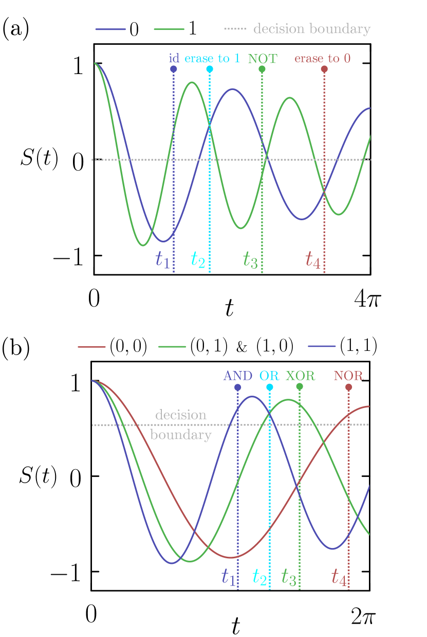
Figure 1: (a) The time-resolved dynamics (2) of the oscillatory neural unit (1), evaluated for the two distinct values of a binary input $I=0,1$. Depending on the observation time $t$, the unit can perform any of the elementary one-bit operations. (b) The time-resolved dynamics of the same neuron, now evaluated for the three distinct values $I=I_{1}+I_{2}=0,1,2$ of the binary inputs $(I_{1},I_{2})$. Depending on the observation time $t$, the unit can function as any of the elementary logic gates. Neuron parameters: $\omega_{0}=1,\gamma=1/10$.

II Time-resolved computation is multifunctional

In more detail, consider a continuous degree of freedom $S(t)$ of unit mass that evolves according to the underdamped Langevin dynamics $\ddot{S}=-\gamma\dot{S}-\partial_{S}U+\eta(t)$. Here $\gamma$ is a friction coefficient, $U$ is a potential, and $\eta$ is a noise term. We will consider the harmonic potential $U=\frac{1}{2}(\omega_{0}^{2}+I)S^{2}$, where $\omega_{0}^{2}$ is the fundamental frequency of the oscillator and $I$ is the input signal (the input signal could in general be time-dependent, but here we consider a constant input). The input therefore influences the spring constant of the harmonic potential. In general, thermal noise provides an important mechanism for driving dynamical evolution and allowing probabilistic computation Aifer et al. (2023). Here, for simplicity, we assume the low-noise limit, and so the oscillator evolves according to the equation

$$\ddot{S}+\gamma\dot{S}+(\omega_{0}^{2}+I)S=0.$$ (1)

We assume that the oscillator is prepared with initial conditions $S(0)=1$ and $\dot{S}(0)=0$. Then $S$ satisfies

$$S(t)={\rm e}^{-\gamma t/2}\left(\cos\Omega t+\frac{\gamma}{2\Omega}\sin\Omega t\right),$$ (2)

where

$$\Omega^{2}\equiv\omega_{0}^{2}-\gamma^{2}/4+I$$ (3)

is a function of the oscillator’s intrinsic parameters and the input $I$. The input therefore influences the period $2\pi/\Omega$ of the oscillator (we assume the underdamped regime, where $\Omega^{2}>0$). At fixed time the output of the unit is a nonmonotonic function of $I$, and at fixed $I$ the output of the unit is a nonmonotonic function of $t$. These two properties give this neural unit the ability to solve nonlinearly separable problems, and to do so in a temporally multifunctional way.

A neural unit that evolves in time can perform computations in a multifunctional way. Consider a binary input $I=0,1$. In Fig. 1(a) we show the neuron output (2) as a function of time $t$ for the two possible values of $I$. With a horizontal decision boundary placed at zero, the neuron can perform any of the elementary one-bit operations, depending on observation time: identity ($I\to I$) at $t_{1}$; erase to one ($I\to 1$) at $t_{2}$; NOT or invert ($I\to\bar{I}$) at $t_{3}$; and erase to zero ($I\to 0$) at $t_{4}$. The same operations are also performed at other times in the unit’s trajectory.

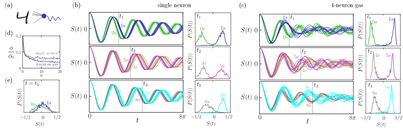
Figure 2: Time-dependent multifunctional classification. (a) An oscillator neuron (1) with $N=28^{2}$ adjustable input weights is shown MNIST digits in classes $0,1,4,5,8$, and 9. Its weights are adjusted by gradient descent to distinguish 0s and 1s at time $t_{1}$; to distinguish 4s and 5s at time $t_{2}$; and to distinguish 8s and 9s at time $t_{3}$. (b) Time traces of the activity of the trained neuron when shown 10 test-set digits (unseen during training) of each indicated class, and histograms of activity (using all digits of that class in the MNIST test set) at the indicated times. (c) As (b), but for a noninteracting gas of 4 neurons, with the 4$N$ input weights adjusted by gradient descent to perform the same multi-time classification task. All histograms have a common vertical scale. (d) Loss (4), scaled by $\phi_{0}=3N_{\rm batch}$, as a function of training epoch $n$. (e) Activity histogram of the neural gas (when shown 0s and 1s) at a time at which it is not trained to discriminate 0s and 1s. Neuron parameters: $\omega_{0}=1,\gamma=1/10$.

Conventional physical models of processes such as bit erasure consider the manipulation of a degree of freedom in an external potential, with work expended Landauer (1961); Sagawa (2012); Zulkowski and DeWeese (2014); Proesmans et al. (2020); Dago and Bellon (2022). Here, energy must be input in order to set the initial state of the unit and impose and maintain the input to the neuron (which sets the potential spring constant). But after setting the initial condition no work is performed: computations are done by the system’s natural dynamics .

Now consider two binary input degrees of freedom $I_{1,2}=0,1$, and construct the input $I=I_{1}+I_{2}$. $I$ can take three values, 0,1, or 2. In Fig. 1(b) we show the neuron output (2) as a function of time $t$ for the three possible values of $I$. With the horizontal decision boundary placed as shown, the neuron can function as any of the elementary logic gates, depending on observation time. If we observe the unit at time $t_{1}$ it functions as an AND gate; at time $t_{2}$, an OR gate; and at time $t_{3}$, an XOR gate. At different times the same unit can also function as the inverted versions of these gates, NAND, XNOR, and NOR, the latter shown at time $t_{4}$.

The equilibrium state of the unit is $S(t\to\infty)=0$, regardless of the value of $I$, and so in equilibrium the unit has no computational ability. In general, we can do time-resolved computation in or out of equilibrium, but doing it out of equilibrium means that we do not need to wait for equilibrium to be attained.

III Training oscillator neurons to perform multifunctional computation

Dynamical oscillator neurons can be trained by gradient descent to achieve distinct tasks at distinct times. To illustrate this point we consider the MNIST data set LeCun et al. (1998), which consists of greyscale images of handwritten digits on a grid of $N=28\times 28$ pixels, each digit belonging to one of ten classes $C\in[0,9]$; see Fig. 2(a). We wish to construct a classifier that discriminates 0s (class $C=0$) from 1s (class $C=1$) at observation time $t_{1}$; discriminates 4s from 5s at time $t_{2}$; and discriminates 8s from 9s at time $t_{3}$. We choose observation times $t_{1}$, $t_{2}$, and $t_{3}$ such that $\Omega_{0}t_{k}=-\arctan(2\Omega_{0}/\gamma)+(k+3)\pi$, where $\Omega_{0}^{2}\equiv\omega_{0}^{2}-\gamma^{2}/4$, corresponding to three of the roots of the function (2) with $I=0$.

A loss function suitable for this multi-time classification task is

$$\phi=\sum_{k=1,2,3}\sum_{\alpha\in C_{4k},C_{4k+1}}(s_{\alpha}(t_{k})-\bar{s}_{\alpha})^{2}.$$ (4)

Here $\alpha$ labels MNIST digits, and the inner sum runs over training-set digits in classes $C_{4k}$ and $C_{4k+1}$. We have defined $s_{\alpha}(t_{k})\equiv{\rm e}^{\gamma t/2}S_{\alpha}(t_{k})$; the exponential scaling cancels the exponential decay of the solution (2), ensuring that each term in (4) is of equal importance. $S_{\alpha}(t_{k})$ denotes the value of (2) at time $t_{k}$ when shown MNIST digit $\alpha$. We consider $N$ connections between digit and neuron: when shown digit $\alpha$, the neuron input is $I_{\alpha}=\sum_{i=1}^{N}\theta_{i}I_{i,\alpha}$, where $I_{i,\alpha}$ is the value of the $i^{\rm th}$ pixel of MNIST digit $\alpha$ and the $N$ quantities $\theta_{i}$ are adjustable weights. In what follows we use the notation $\Omega_{\alpha}^{2}\equiv\omega_{0}^{2}-\gamma^{2}/4+I_{\alpha}$. The target activity in (4) is $\bar{s}_{\alpha}=\mp 1/2$, where the negative or positive sign is chosen if digit $\alpha$ is a member of an even-numbered class $(0,4,8)$ or an odd-numbered class $(1,5,9)$, respectively.

To train the neuron to solve this multi-time classification task we adjust its input weights by gradient descent on $\phi$. Weights are initially chosen randomly, $\theta_{i}\sim{\mathcal{N}}(0,10^{-4})$; we then iterate the equation $\theta_{i}\to\theta_{i}-\alpha_{0}\partial\phi/\partial\theta_{i}$ for all $N$ weights $\theta_{i}$. Here $\alpha_{0}$ is the learning rate and

$$\frac{\partial\phi}{\partial\theta_{i}}=\sum_{k=1,2,3}\sum_{\alpha\in C_{4k},C_{4k+1}}(s_{\alpha}(t_{k})-\bar{s}_{\alpha})g(t_{k},\Omega_{\alpha})I_{i,\alpha},$$ (5)

where

$$g(t,\Omega)\equiv\frac{\gamma t}{2\Omega^{2}}\cos\Omega t-\frac{1}{\Omega}\left(t+\frac{\gamma}{2\Omega^{2}}\right)\sin\Omega t.$$ (6)

We take the inner sum in (5) over stochastically-chosen minibatches of $N_{\rm batch}=300$ digits, split equally between classes $C_{4k}$ and $C_{4k+1}$. We set the learning rate to $\alpha_{0}=10^{-3}(3N_{\rm batch})^{-1}$ .

Results are shown in Fig. 2(b). We plot time traces of neuron activity when shown 10 test-set digits (unseen during training) in each class. Classes are indicated by color. The neuron responds differently to each class, and can (imperfectly) distinguish the required classes at the required times: on the right of the panel we show histograms of neuron activity, using all digits of that class in the MNIST test set, at the designated observation times.

As with standard neural units, collections of oscillator neurons are more expressive than individual neurons. Multiple oscillator neurons can have a total activity that is not periodic in time, even if they do not interact. In Fig. 2(c) we show the analog of panel (b) for a collection of 4 noninteracting neurons. Each has the same parameters $\omega_{0}$ and $\gamma$ as the single neuron of panel (b), and each has $N$ input weights. We impose the loss function $\phi$, with $S_{\alpha}(t)$ replaced by $\frac{1}{4}\sum_{i=1}^{4}S^{(i)}_{\alpha}(t)$. Here $S^{(i)}_{\alpha}(t)$ is the output of neuron $i$ at time $t$ when shown MNIST digit $\alpha$. As before, we adjust the input weights by gradient descent on the loss.

The time traces and histograms of Fig. 2(c) show the trained neural gas to be more expressive than the trained individual neuron, better distinguishing the required classes at the designated observation time (the loss values for the individual neuron and the gas are shown in Fig. 2(d)). In panel (e) we show histograms of neural activity at a time $t_{3}$ for which the neural gas is trained to discriminate 8s and 9s but not 0s and 1s; there, it cannot distinguish 0s and 1s.

IV Conclusions

Several branches of computing use the natural evolution of a physical system to do calculations. We have shown that the dynamics of an underdamped harmonic oscillator can perform multifunctional computation, with the same physical system able to solve distinct problems at distinct times within a single dynamical trajectory. The idea proposed here, a form of analog computing, is a nonstandard form of oscillator computing: the latter usually focuses on the information contained within the phase of an oscillator, and seeks to identify the ground-state phases of coupled oscillators. Here we have considered the time-resolved amplitude of an oscillator whose inputs influence its frequency, which we interpret as a time-dependent neural unit. The activity of the unit at fixed time is a nonmonotonic function of the input, and so it can solve nonlinearly-separable problems such as XOR. The activity of the unit at fixed input is a nonmonotonic function of time, and so the unit is multifunctional in a temporal sense, able to carry out distinct nonlinear computations at distinct times within the same dynamical trajectory. We have shown that such units can function as all of the elementary logic gates, depending on observation time, and have shown how to train such units by gradient descent to perform distinct classification tasks at distinct times.

A single temporal oscillator neuron can do nonlinear computation in a multifunctional way, and is a natural building block for neural networks and other devices. Neural networks can be built from interacting oscillators just as they are built from standard artificial neurons Effenberger et al. (2022). Oscillator neural nets designed for multifunctional computation would have considerable computational power, particularly if the connections between neurons were designed to make efficient use of the multiple distinct computations done by neurons at distinct times.

The idea described here does not require thermal noise but could be applied in its presence: in fields such as thermodynamic computing, thermal noise provides an important mechanism for driving dynamical evolution and allowing probabilistic computation Aifer et al. (2023). The results of this paper suggest extending the idea of thermodynamic computing to consider the time-resolved dynamics of devices that already exist, such as networks of interacting oscillators printed on circuit boards Wang and Roychowdhury (2019); Chou et al. (2019); Melanson et al. (2023).

Time-resolved multifunctional computing provides a way of carrying out multiple nonlinear computations within a single dynamical trajectory of a device. This idea could help reduce the number of parameters or the size of devices needed to do computation, with the natural time evolution of a device giving us, in effect, multiple computations for the price of one.

V Acknowledgments.

I thank Isaac Tamblyn for comments on the paper. This work was done at the Molecular Foundry at Lawrence Berkeley National Laboratory, supported by the Office of Basic Energy Sciences of the U.S. Department of Energy under Contract No. DE-AC02–05CH11231.

References

- Bennett (1982) C. H. Bennett, International Journal of Theoretical Physics 21, 905 (1982).
- Landauer (1991) R. Landauer, Physics Today 44, 23 (1991).
- Wolpert (2019) D. H. Wolpert, Journal of Physics A: Mathematical and Theoretical 52, 193001 (2019).
- Ceruzzi (2003) P. E. Ceruzzi, A history of modern computing (MIT press, 2003).
- Horowitz and Grumbling (2019) M. Horowitz and E. Grumbling, (2019).
- Schuman et al. (2017) C. D. Schuman, T. E. Potok, R. M. Patton, J. D. Birdwell, M. E. Dean, G. S. Rose, and J. S. Plank, arXiv preprint arXiv:1705.06963 (2017).
- Sun et al. (2020) C. Sun, M. Song, S. Hong, and H. Li, arXiv preprint arXiv:2012.02974 (2020).
- MacLennan (2007) B. J. MacLennan, Department of Electrical Engineering & Computer Science, University of Tennessee, Technical Report UT-CS-07-601 (September) , 19798 (2007).
- Ulmann (2013) B. Ulmann, Analog computing (Oldenbourg Wissenschaftsverlag Verlag, 2013).
- Csaba and Porod (2020) G. Csaba and W. Porod, Applied physics reviews 7 (2020).
- Conte et al. (2019) T. Conte, E. DeBenedictis, N. Ganesh, T. Hylton, J. P. Strachan, R. S. Williams, A. Alemi, L. Altenberg, G. Crooks, J. Crutchfield, et al., arXiv preprint arXiv:1911.01968 (2019).
- Hylton (2020) T. Hylton, in Proceedings, Vol. 47 (MDPI, 2020) p. 23.
- Aifer et al. (2023) M. Aifer, K. Donatella, M. H. Gordon, T. Ahle, D. Simpson, G. E. Crooks, and P. J. Coles, arXiv preprint arXiv:2308.05660 (2023).
- Von Neumann (1957) J. Von Neumann, “Non-linear capacitance or inductance switching, amplifying, and memory organs,” (1957), US Patent 2,815,488.
- Ciliberto (2017) S. Ciliberto, Physical Review X 7, 021051 (2017).
- Dago et al. (2021) S. Dago, J. Pereda, N. Barros, S. Ciliberto, and L. Bellon, Physical Review Letters 126, 170601 (2021).
- Dago et al. (2022) S. Dago, J. Pereda, S. Ciliberto, and L. Bellon, Journal of Statistical Mechanics: Theory and Experiment 2022, 053209 (2022).
- Wang and Roychowdhury (2019) T. Wang and J. Roychowdhury, in Unconventional Computation and Natural Computation: 18th International Conference, UCNC 2019, Tokyo, Japan, June 3–7, 2019, Proceedings 18 (Springer, 2019) pp. 232–256.
- Chou et al. (2019) J. Chou, S. Bramhavar, S. Ghosh, and W. Herzog, Scientific Reports 9, 14786 (2019).
- Melanson et al. (2023) D. Melanson, M. A. Khater, M. Aifer, K. Donatella, M. H. Gordon, T. Ahle, G. Crooks, A. J. Martinez, F. Sbahi, and P. J. Coles, arXiv preprint arXiv:2312.04836 (2023).
- Goto (1959) E. Goto, Proceedings of the IRE 47, 1304 (1959).
- Bonnin et al. (2022) M. Bonnin, F. L. Traversa, and F. Bonani, Advances in Artificial Intelligence-based Technologies: Selected Papers in Honour of Professor Nikolaos G. Bourbakis-Vol. 1 , 179 (2022).
- Rumelhart et al. (1986) D. E. Rumelhart, G. E. Hinton, and R. J. Williams, Biometrika 71, 599 (1986).
- Gidon et al. (2020) A. Gidon, T. A. Zolnik, P. Fidzinski, F. Bolduan, A. Papoutsi, P. Poirazi, M. Holtkamp, I. Vida, and M. E. Larkum, Science 367, 83 (2020).
- Noel et al. (2021) M. M. Noel, S. Bharadwaj, V. Muthiah-Nakarajan, P. Dutta, and G. B. Amali, arXiv preprint arXiv:2111.04020 (2021).
- Effenberger et al. (2022) F. Effenberger, P. Carvalho, I. Dubinin, and W. Singer, bioRxiv , 2022 (2022).
- Landauer (1961) R. Landauer, IBM journal of research and development 5, 183 (1961).
- Sagawa (2012) T. Sagawa, Progress of theoretical physics 127, 1 (2012).
- Zulkowski and DeWeese (2014) P. R. Zulkowski and M. R. DeWeese, Physical Review E 89, 052140 (2014).
- Proesmans et al. (2020) K. Proesmans, J. Ehrich, and J. Bechhoefer, Physical Review Letters 125, 100602 (2020).
- Dago and Bellon (2022) S. Dago and L. Bellon, Physical Review Letters 128, 070604 (2022).
- Note (1) Single operations and multiple operations incur the same energy cost, with the caveat that the input to the neuron must be maintained long enough to observe these operations.
- LeCun et al. (1998) Y. LeCun, L. Bottou, Y. Bengio, and P. Haffner, Proceedings of the IEEE 86, 2278 (1998).
- Note (2) It could happen during training that becomes negative for certain , indicating overdamping, in which case we must make the replacement in (2) and (6). This did not happen in the simulations reported here.