Boundary determination and local rigidity of analytic metrics in the Lorentzian scattering rigidity problem
Abstract.
We study the scattering rigidity problem in Lorentzian geometry: recovery of a Lorentzian metric from the scattering relation known on a lateral timelike boundary. We show that one can recover the jet of the metric up to a gauge transformation near a lightlike strictly convex point. Assuming that the metric is real analytic, we show that one can recover the metric up to a gauge transformation as well near such a point.
1. Introduction
Let be a Lorentzian manifold of dimension with a cylindrical-like timelike boundary, generalizing where is a compact Riemannian manifold with a smooth boundary. We define the (lightlike) scattering relations , and , acting on vectors and covectors, respectively, as the exit points and directions/codirections on the boundary of lightlike geodesics starting at such points and directions/codirections at the boundary, see Definition 2.1 for a precise statement. The problem we study is to what extent does or determine . In this generality the problem is wide open with some partial results so far described below. In this paper we show that one can recover the whole jet of on , assumed strictly convex to light rays, up to a gauge transformation. Also, if is a priori analytic, one can recover in near such points.
The lightlike probes the metric over a restricted set of geodesics, satisfying . This takes one dimension away from the set of all geodesics, and, together with the signature of the metric, makes the Lorentzian version of this problem harder with new challenges. First, the group of the gauge transformations is richer, since it adds the freedom to multiply by an arbitrary (positive) conformal factor . In fact, it is arbitrary for with the additional restriction on for . Next, the linearization of this problem is the geodesic light ray transform [24], which is known to be unable to see timelike singularities; roughly speaking those corresponding to signals moving faster than light. A loss of ellipticity exists in the Riemannian case as well when , and we restrict ourselves to “short” geodesics close to being tangent to the boundary, but it is of a different nature. Then it is not a priori intuitively clear in the Lorentzian case whether one can expect boundary or local/global recovery, the latter even in the analytic case, but we show that the local recovery is possible.
One possible motivation to study comes from the analysis of the wave equation related to . As it was shown in [30], is the canonical relation of the Dirichlet-to-Neumann map on , which is a Fourier Integral Operator. From relativity point of view, and contains information about the way photon trajectories are affected by the Lorentzian structure of spacetime. A linearization of from a spacelike hypersurface (“shortly” after the Big Bang) to a future one (the present) is studied in [11], motivated by the information carried by the observed redshift of the cosmic background radiation.
Boundary determination results for Riemannian manifolds with boundary are well known [12], including stability estimates [26], and a constructive algorithm [32]. The strict convexity condition was relaxed considerably to include concave points under a certain non-conjugacy condition in [27], see also [35]. As a consequence, Vargo [34] showed that one can recover an analytic non-trapping Riemannian manifold up to an isometry from the lens relation. This result was extended in [10] to such manifolds with an analytic magnetic field. A major advancement in dimensions was done in [28, 29] based on the approach in [31], where it was shown that for smooth metrics, we can recover not just the jet of on the boundary up to a gauge, but inside as well, near a strictly convex point. This implies global rigidity results under a foliation condition. The approach is based on ellipticity of the linearization (and on the use of Melrose’s scattering calculus) which does not hold in our case.
There are many boundary and lens/scattering rigidity results in the Riemannian case, aside from the already mentioned [28, 29] see, e.g., [27, 26, 25, 21, 16, 15, 14, 13, 12, 9, 4, 5, 2, 3, 1]. They can be viewed as rigidity results for static Lorentzian metrics. Very little is known in the Lorentzian case. Recovery of stationary metrics from the time separation function was studied in [33]. The author showed in [24], that under some additional conditions, stationary metrics in cylindrical product type of manifolds with boundary are lens rigid near a generic set of simple metrics, including simple real analytic ones. The reason for this is that projected onto the “base” , such systems reduce to magnetic ones studied before in [6]. Scattering rigidity via timelike geodesics was studied in [19] for stationary metrics. The dynamical system then projects to a magnetic-potential one studied in [18, 17]. Our second main result is that assuming real analytic, it is uniquely determined by near strictly lightlike convex boundary points.
Brief description of the approach. To explain the challenges, we note first that we need to prove the existence of a gauge transformation, see Definition 2.2 relating two metrics and with the same data. That means construction of two quantities: a diffeomorphism and a conformal factor . In the Riemannian case, we have only, and it is a priori clear what it should be near , if there is rigidity: just identify the boundary normal coordinates for and . Then we need to prove that up to infinite order at with known. One way to do this is as in [12] by looking at the Taylor expansion of in the normal variable . We do not have such natural candidates for and in the Lorentzian case. To construct such candidates, we “normalize” first and in the gauge equivalent class, see section 4.1: to coincide on some timelike field tangent to ; and at the same time to be both in boundary normal coordinates, both up to , as . This leads to a non-characteristic Cauchy problem for a fully nonlinear PDE, see (4.6), which can be transformed easily into a quasilinear one, see (5.1). It is not a priori clear that this problem is solvable but it can always be solved up to . Once we have this, we apply the Taylor series argument using the maximizing property of timelike geodesics.
Assuming the metrics analytic, one would think that one can just use analytic continuation. That is essential for this result, of course, but we need to show that and which we constructed only up to an infinite order at , actually exist locally. We apply the Cauchy–Kowalevski theorem to show that the “normalization” in section 4.1 can be done exactly, locally, allowing us to construct and locally. Then we use analytic continuation.
One could hopefully prove global rigidity results for analytic metrics under appropriate geometry conditions but that would require some non-trivial efforts, and will be studied in a forthcoming work.
Acknowledgments. The author thanks Leo Tzou and Lauri Oksanen for an inspiring discussion on related problems, and to Sebastián Muñoz-Thon for his critical remarks.
2. Main results
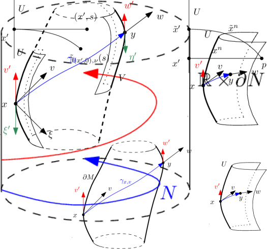
We start with the introduction of the main notions, see also [24]. Let , with timelike, and let be a lightlike vector at pointing into . Assume that the lightlike geodesic hits again for the first time for some , at in the direction . We can define the scattering relation as the map , see Figure 1.
It is convenient to identify such lightlike vectors with their orthogonal projections to . Those projections would be timelike, and in the limiting case when is tangential to , they would be lightlike. Recall that vectors that are either timelike of lightlike are called causal. Then we can think of the scattering relation as defined on the causal cone in with an image in the causal cone in unless the corresponding geodesic is trapping.
This leads to the following.
Definition 2.1.
The scattering relation , mapping the causal cone in to itself, is defined as follows. Let be timelike, and let be the unique lightlike vector at with orthogonal projection on , pointing to the interior of . Then we set to be the point where the geodesic issued from meets again for the first time, and set to be the orthogonal projection on of its direction there. We set .
When is lightlike, is tangent to , and we set .
The scattering relation on the causal cone in is defined as by identifying vectors and covectors by the metric.
We use the musical isomorphism notation below converting vectors to covectors and vice versa.
If happens to be trapping for some , we just consider that not to be in the domain of (and this is not going to be allowed in this paper). Knowing or includes knowing the domain.
Clearly, and are positively homogeneous of order one in the fiber variable. We have for every . We may normalize in some way to reduce the number of variables. For example, if is a local time variable, we may require .
One can view as the actual observable instead of . The projection of either or on in the metric can be viewed as the projections of their covector versions , , respectively, on with respect to the pairing of a covector and a vector. That does not require the knowledge of on . Also, as the author and Yang showed in [30],
The definition of or requires us to know which vectors/covectors on the boundary are causal, which is equivalent to knowing a conformal multiple of restricted to . Instead of prescribing or , we can consider the pairs of points in which can be connected by a lightlike geodesic, so that and are not conjugate along it. It was shown in [24] that and determine each other uniquely. We take as our data to avoid prescribing on the boundary.
Definition 2.2.
We call and gauge equivalent, if there exists a diffeomorphism fixing pointwise, and a function , so that . When studying a local version of or , we assume that and are defined in the open set of covered by the geodesic used in the definition of .
Fixing a positive sign of the conformal factors, as we did, preserves the signature of the metric. We showed in [24] that gauge equivalent Lorentzian metrics on the same manifold have the same . The relation , on the other hand, is affected by on , and gauge transformations preserve of on . In both cases, the gauge transformations form a group generated by conformal multiples and isometries fixing pointwise.
We define the notion of strict convexity as in [23].
Definition 2.3.
Let be a smooth hypersurface near a point and let be a defining function so that near , , and declare , to be the “interior” of near . Similarly, is the “exterior” of near . We say that is strictly convex at in the direction , if .
Strict convexity of for restricted to a set of null vectors can be defined in a similar way. In this paper, the directions would be lightlike, and we call this strict lightlike convexity.
Here is the Hessian of , with being the covariant derivative. This notion of strict convexity at is equivalent to for the geodesic through in the direction ; and it is independent of the choice of . When , the interior is , and the exterior does not exist. We can extend smoothly on the other side of however, and then this characterization still holds independently of the extension.
Our first main result is boundary recovery for smooth metrics.
Theorem 2.1 (Boundary Recovery).
Let and be two Lorentzian metrics defined near some so that on locally with some . Let be lightlike for . Assume that is strictly convex with respect to in the direction of . Assume that either
-
(i)
in a neighborhood of , or
-
(ii)
in a neighborhood of , and .
Then there exists with on , and a local diffeomorphism near preserving it pointwise, so that the jets of and coincide on near .
Next, we prove local rigidity for analytic manifolds and metrics. Analyticity always means real analyticity in this paper, and analyticity in always means analyticity up to the boundary, i.e., existence of an analytic extension in some two-sided neighborhood of , where is assumed to have an analytic extension as well. Similarly, analyticity near means analyticity in a two-sided neighborhood of in the extended .
Theorem 2.2 (Local rigidity for analytic metrics).
3. Preliminary results
3.1. Gauge transformations
We review some results from [24]. Recall that multiplying by a conformal factor reparameterizes the future directed null geodesics, keeping the future orientation, but leaves them the same as point sets [11, 24]. This extends easily to more general Hamiltonians and to depending on both and . Next lemma is stated in a greater generality than we need it.
Lemma 3.1.
Let be a Hamiltonian defined near , and assume , . Let near . Then the Hamiltonian curves of and near on the zero energy level coincide as point sets but have possibly different parameterizations.
More specifically, if , and are solutions related to and , with initial conditions at , and at , , respectively, then
with solving
Proof.
The Hamiltonian system for related to reads
Assume initial conditions at . On the energy level , we are left with
Then for we get the Hamiltonian system related to with initial conditions as stated above. This completes the proof. ∎
We apply the lemma to the Hamiltonian , written in local coordinates. It is well known that the Hamiltonian curves of on at zero energy level, when identified with curves in by the musical isomorphism, coincide with the lightlike geodesics. When , the corresponding Hamiltonian is . Then
with solving
This shows that is invariant under the conformal transformation . Indeed, is unchanged, see Figure 1. Next, has the unique decomposition , where , and is conormal to , i.e., normal to all covectors in in the metric . This decomposition does not change when we replace by . Therefore, the projection is independent of the conformal factor, and the same applies to at . Thus is independent of a conformal transformation. On the other hand, when on , one can multiply either metric by with on only to preserve that condition.
Those arguments apply to the vectors and as well but there is an essential difference. The map , before the projections, does depend on because the musical isomorphism converting into , and similarly for and brings the factor . Indeed, assume now. Then can be computed as
With , we have , and can be computed as
Therefore,
see also in [11, eq. (17)]. Therefore, is preserved under the conformal change if and only if for all , which implies on . Moreover, if on , then the condition is . Under the conditions of Theorem 2.1, when on , and they have the same scattering relation, the conformal freedom we have is to multiply one of the metrics by with on which preserves the boundary condition, and it is the conformal factor allowable to preserve . Then we get the same condition as that for but for two reasons, instead for one.
Note however that for two metrics, implies for every .
On the other hand, any diffeomorphism with on preserves both and . It intertwines with multiplying by a conformal factor without changing its boundary values.
3.2. Jets of tensors fields
We fix a small neighborhood of , reserving the right to shrink it several times during the proof. We use coordinates , in near , where is given locally by with in . Given a tensor field of type (metric-like), the jet of on the hypersurface in such a local chart is given by on for all . Knowing the jet of implies knowing all derivatives of at , not just the ones. Under a change of variables, aside from having new variables, changes its coordinate representation as well. The following lemma shows that knowing the jet is a coordinate independent notion.
Lemma 3.2.
Let and be two type tensor fields with the same jets at near in some local coordinates. Let be a local diffeomorphism near the origin so that is mapped to . Then and have the same jets on in the variables.
Proof.
It is enough to assume that . We have
On we have , which implies the same for . More generally, applying any, say constant coefficient (in the variables) differential operator to the left-hand side, yields zero on the right on the same hypersurface since the jet of is zero there. ∎
In particular, we can take fixing pointwise locally, i.e., , , and . Then two tensor fields having the same jet at is equivalent to having the same same derivatives of every order under any such change.
3.3. Boundary normal coordinates
Lorentzian manifolds with boundary admit boundary normal coordinates similarly to Riemannian ones. The following lemma is formulated in [30] but the proof is in [22]. It is based on the fact that the lines , are unit speed geodesics; therefore the Christoffel symbols vanish for all .
Lemma 3.3.
Let be a timelike hypersurface in . For every , there exist , a neighborhood of in , and a diffeomorphism such that
(i) for all ;
(ii) where is the unit speed geodesic issued from normal to .
Moreover, if are local boundary coordinates on , in the coordinate system , the metric tensor takes the form
| (3.1) |
Clearly, has a Lorentzian signature as well. If has a boundary, then can be and is restricted to . We will call such coordinates the boundary normal coordinates. The lemma remains true if is spacelike with a negative sign in front of in (3.1) (we replace the index by below), and this gives us a way to define a time function locally, and put the metric in the block form
| (3.2) |
with Riemannian.
3.4. Tensor fields vanishing on the lightlike cone
Lemma 3.4.
Let be a tensor such that for all lightlike for the metric , with both and constant. Then with some constant .
Proof.
Applying a Lorentzian transformation, we can always assume that is Minkowski. In fact, such a transformation would produce the Minkowski metric times a conformal factor. Take . Expanding in Fourier series in , we get
This implies , , i.e., the block of is conformal to the Minkowski one, with conformal factor -. We can put and in any two different positions different from the zeroth one to complete the proof.
An alternative proof is to identify the conformal factor as first, if is Minkowski. Then for , we get
for all unit in the Euclidean norm. By [6, Lemma 3.3], this implies . ∎
As a consequence, if and depend on , and for all lightlike near a fixed , we can extend this to all based at those points by analyticity on (and the proof is local in anyway), and we get the conclusion in the lemma with having the regularity of and : smooth or analytic.
4. Recovery of the jet at the boundary
We prove Theorem 2.1 in this section.
4.1. Step 1: “Normalizing” and
Recall the coordinate convention of section 3. We assume that (not to be confused with the point ) is a local time coordinate, i.e, . We will choose a metric , gauge equivalent to such that it has the form (3.1) up to with respect to the same boundary normal coordinates related to , and it coincides with on in up to . We use the freedom to make conformal changes at this step but we do not use the equality of the scattering relations yet.
We normalize and first conformally assuming
| (4.1) |
This can be easily achieved by dividing by with extended in near . This does not change the data in either case, or and allows us to assume . Then we pass to (3.1) with respect to , which does not affect (4.1). We do the same for , assuming at this point that are common boundary normal coordinates for both and .
We want and to solve
| (4.2) |
up to with boundary conditions on , on . The conversion to common boundary normal coordinates guarantees (4.2) on only. From now on, we assume that Greek indices run from to while Latin ones run from to . Equation (4.2) is equivalent to
| (4.3) | ||||
| (4.4) |
up to again. This is an system for but there are no derivatives of involved. The boundary condition is
| (4.5) |
The latter condition is automatically satisfied if the former is, as a consequence of (4.3) and (4.1). We can eliminate in (4.4) and (4.3) to get the fully nonlinear first order system
| (4.6) |
for equivalent to (4.4) by (4.3) since having , we can solve for in (4.3).
We will prove that the boundary is non-characteristic for (4.6), (4.5). We show first that one can determine the jet of at locally, under the additional assumption at . Differentiating (4.5) with respect to , we get , , at . In particular, the right-hand side of (4.6) equals . We can write (4.6) at as , which means that is orthogonal to the basis vectors , , and unit. This implies at . Note that this is consistent with the geometric construction of which, combined with (4.1) implies , i.e.,
| (4.7) |
In particular, is a diffeomorphism near .
Therefore, we can find a solution of (4.2), (4.5) up to . Note that the usual argument is that if a solution exists, we can compute the Taylor expansion at the boundary. The same arguments show that an asymptotic solution actually exists, even if we do not know that an exact one does (and this argument is used in the proof of the Cauchy Kowalevsky theorem).
We replace by the gauge equivalent . Then we have
| (4.8) |
Recall the boundary conditions (4.1). We want to prove that
| (4.9) |
for near .
4.2. Step 2: is strictly convex with respect to as well
The geodesic equation implies
| (4.10) |
Recall that which is implied by the property , . In the coordinates in Lemma 3.3, , which is also the second fundamental form of . Strict convexity at is equivalent to . It is positive definite along vectors close to by assumption. We can assume that the metric is Minkowski at . We take lightlike, pointing to the interior of , so that it converges to , as . We do this by taking with unit in ; then . Then for the -th component of the geodesic through , with initial direction , we have
| (4.11) |
The function then has a non-negative zero for . We can think of it as an escape “time.” Then reaches again for .
Let be the first intersection point of the geodesic with (not counting the initial point ). Then
| (4.12) |
Since is identity at the origin, we get the same asymptotic expansion for in the so chosen local coordinates.
We will show that is strictly convex at with respect to as well. Since on by (4.1), we know that is lightlike for as well. By (4.8), the lightlike vector at pointing into , related to , is still . Then (4.11) still holds with replaced by with the hat over a quantity indicating that it is related to . Note that are (exact) boundary normal coordinates for only, and only such up to with respect to by (4.8) but this does not affect our argument. Since or , still has a positive zero at , which implies ; thus is strictly convex at , and therefore near it as well, with respect to as well.
4.3. Step 3: recovery of the jet of the metric
In preparation for the final step, assume that (4.9) does not hold. Then near with some symmetric tensor field not vanishing at , and with some . By (4.8), , , . By Lemma 3.4, if we prove that for all lightlike for , close to , then we would get with some . Then by (4.2); therefore , and then . That would be a contradiction.
Assume . Without loss of generality, we can assume ; if the opposite, we can switch and below. Then for in the interior of (but not on ) close enough to , and for close enough to . With as above, let and be the lightlike geodesics in the metrics and , respectively, connecting and . By what we assumed, is a timelike curve in the metric except for the endpoints, where it is lightlike. Assume it is parameterized by . Consider the points , with . If , those two points are connected by the timelike (for ). By [20, Proposition 5.34], the “radial” geodesic segment (in the metric , again) between those two points is the unique longest timelike curve connecting them. We recall that the radial geodesic connecting and is the geodesic from with direction , assuming the inverse exponential map is well-defined; and we restrict the considerations close to . Passing to the limit , we get that the length of has an upper limit because the unique timelike geodesic in the proposition tends to , which is lightlike. Thus we get that is lightlike for as well; in particular and coincide as point sets. This contradicts our assumption. We can perturb a bit keeping it lightlike for . Perturbing now, we get that on . Then we get the needed contradiction.
This completes the proof of Theorem 2.1.
5. Local rigidity for analytic metrics
Proof of Theorem 2.2.
We return to the system (4.3), (4.4), (4.5), this time with the analyticity assumptions. As explained in section 4.1, the system can be reduced to (4.6), (4.5), and after solving for , we determine from (4.3). The reduced system has analytic coefficients near when the original system is analytic, including on extended analytically to near . To make the boundary condition homogeneous, we set . Then, see also section 4.1, we recast (4.6) as
| (5.1) |
with Cauchy data
| (5.2) |
As we showed in section 4.1, (5.1), (5.2) is solvable at near assuming , which allows us to take the positive sign of the square root to determine . This means that we can write it as
with an -vector valued function satisfying ; analytic near under our analyticity assumptions. By the Cauchy–Kowalevski theorem, see [7, 8], there exists an unique, in the class of analytic functions, local solution of (5.1), (5.2), near . Then there is an analytic solving (4.6), (4.5) near as well; and then we can determine , also analytic, locally by (4.3) as well since . Then (4.2) is satisfied locally as well. The jets of and coincide near by the results of section 4, therefore near by analytic continuation. ∎
References
- [1] D. Burago and S. Ivanov. Boundary rigidity and filling volume minimality of metrics close to a flat one. Ann. of Math. (2), 171(2):1183–1211, 2010.
- [2] C. Croke. Scattering rigidity with trapped geodesics. Ergodic Theory Dynam. Systems, 34(3):826–836, 2014.
- [3] C. B. Croke. Rigidity theorems in Riemannian geometry. In Geometric methods in inverse problems and PDE control, volume 137 of IMA Vol. Math. Appl., pages 47–72. Springer, New York, 2004.
- [4] C. B. Croke, N. S. Dairbekov, and V. A. Sharafutdinov. Local boundary rigidity of a compact Riemannian manifold with curvature bounded above. Trans. Amer. Math. Soc., 352(9):3937–3956, 2000.
- [5] C. B. Croke and P. Herreros. Lens rigidity with trapped geodesics in two dimensions. Asian J. Math., 20(1):47–57, 2016.
- [6] N. S. Dairbekov, G. P. Paternain, P. Stefanov, and G. Uhlmann. The boundary rigidity problem in the presence of a magnetic field. Adv. Math., 216(2):535–609, 2007.
- [7] L. C. Evans. Partial differential equations, volume 19 of Graduate Studies in Mathematics. American Mathematical Society, Providence, RI, 1998.
- [8] G. B. Folland. Introduction to partial differential equations. Princeton University Press, Princeton, NJ, second edition, 1995.
- [9] C. Guillarmou. Lens rigidity for manifolds with hyperbolic trapped sets. J. Amer. Math. Soc., 30(2):561–599, 2017.
- [10] P. Herreros and J. Vargo. Scattering rigidity for analytic Riemannian manifolds with a possible magnetic field. J. Geom. Anal., 21(3):641–664, 2011.
- [11] M. Lassas, L. Oksanen, P. Stefanov, and G. Uhlmann. On the Inverse Problem of Finding Cosmic Strings and Other Topological Defects. Comm. Math. Phys., 357(2):569–595, 2018.
- [12] M. Lassas, V. Sharafutdinov, and G. Uhlmann. Semiglobal boundary rigidity for Riemannian metrics. Math. Ann., 325(4):767–793, 2003.
- [13] R. Michel. Sur la rigidité imposée par la longueur des géodésiques. Invent. Math., 65(1):71–83, 1981/82.
- [14] R. G. Muhometov. The reconstruction problem of a two-dimensional Riemannian metric, and integral geometry. Dokl. Akad. Nauk SSSR, 232(1):32–35, 1977.
- [15] R. G. Muhometov. On a problem of reconstructing Riemannian metrics. Sibirsk. Mat. Zh., 22(3):119–135, 237, 1981.
- [16] R. G. Muhometov and V. G. Romanov. On the problem of finding an isotropic Riemannian metric in an -dimensional space. Dokl. Akad. Nauk SSSR, 243(1):41–44, 1978.
- [17] S. Muñoz-Thon. The boundary and scattering rigidity problems for simple MP-systems. arXiv:2312.02506, 2023.
- [18] S. Muñoz-Thon. The linearization of the boundary rigidity problem for mp-systems and generic local boundary rigidity. arXiv:2401.11570, 2024.
- [19] S. Muñoz-Thon. Scattering rigidity for standard stationary manifolds via timelike geodesics. arXiv:2404.09449, 2024.
- [20] B. O’Neill. Semi-Riemannian Geometry With Applications to Relativity, volume 103 of Pure and Applied Mathematics. Academic Press, Inc. [Harcourt Brace Jovanovich, Publishers], New York, 1983.
- [21] L. Pestov and G. Uhlmann. Two dimensional compact simple Riemannian manifolds are boundary distance rigid. Ann. of Math. (2), 161(2):1093–1110, 2005.
- [22] A. Z. Petrov. Einstein Spaces. Translated from the Russian by R. F. Kelleher. Translation edited by J. Woodrow. Pergamon Press, Oxford-Edinburgh-New York, 1969.
- [23] P. Stefanov. Support theorems for the light ray transform on analytic Lorentzian manifolds. Proc. Amer. Math. Soc., 145(3):1259–1274, 2017.
- [24] P. Stefanov. The Lorentzian scattering rigidity problem and rigidity of stationary metrics. arXiv:2212.13213, 2023.
- [25] P. Stefanov and G. Uhlmann. Rigidity for metrics with the same lengths of geodesics. Math. Res. Lett., 5(1-2):83–96, 1998.
- [26] P. Stefanov and G. Uhlmann. Boundary rigidity and stability for generic simple metrics. J. Amer. Math. Soc., 18(4):975–1003, 2005.
- [27] P. Stefanov and G. Uhlmann. Local lens rigidity with incomplete data for a class of non-simple Riemannian manifolds. J. Differential Geom., 82(2):383–409, 2009.
- [28] P. Stefanov, G. Uhlmann, and A. Vasy. Boundary rigidity with partial data. J. Amer. Math. Soc., 29(2):299–332, 2016.
- [29] P. Stefanov, G. Uhlmann, and A. Vasy. Local and global boundary rigidity and the geodesic X-ray transform in the normal gauge. Ann. of Math. (2), 194(1):1–95, 2021.
- [30] P. Stefanov and Y. Yang. The inverse problem for the Dirichlet-to-Neumann map on Lorentzian manifolds. Anal. PDE, 11(6):1381–1414, 2018.
- [31] G. Uhlmann and A. Vasy. The inverse problem for the local geodesic ray transform. Invent. Math., 205(1):83–120, 2016.
- [32] G. Uhlmann and J. Wang. Boundary determination of a Riemannian metric by the localized boundary distance function. Adv. in Appl. Math., 31(2):379–387, 2003.
- [33] G. Uhlmann, Y. Yang, and H. Zhou. Travel time tomography in stationary spacetimes. J. Geom. Anal., 31(10):9573–9596, 2021.
- [34] J. Vargo. A proof of lens rigidity in the category of analytic metrics. Math. Res. Lett., 16(6):1057–1069, 2009.
- [35] X. Zhou. Recovery of the jet from the boundary distance function. Geom. Dedicata, 160:229–241, 2012.