Understanding Hyperbolic Metric Learning through Hard Negative Sampling

Abstract

In recent years, there has been a growing trend of incorporating hyperbolic geometry methods into computer vision. While these methods have achieved state-of-the-art performance on various metric learning tasks using hyperbolic distance measurements, the underlying theoretical analysis supporting this superior performance remains under-exploited. In this study, we investigate the effects of integrating hyperbolic space into metric learning, particularly when training with contrastive loss. We identify a need for a comprehensive comparison between Euclidean and hyperbolic spaces regarding the temperature effect in the contrastive loss within the existing literature. To address this gap, we conduct an extensive investigation to benchmark the results of Vision Transformers (ViTs) using a hybrid objective function that combines loss from Euclidean and hyperbolic spaces. Additionally, we provide a theoretical analysis of the observed performance improvement. We also reveal that hyperbolic metric learning is highly related to hard negative sampling, providing insights for future work. This work will provide valuable data points and experience in understanding hyperbolic image embeddings. To shed more light on problem-solving and encourage further investigation into our approach, our code is available online.

1 Introduction

In computer vision, the central concept of metric learning [71] is to bring similar data representations (positive pairs) closer in the embedding space while separating dissimilar data representations (negative pairs). This approach hinges on the embedding space’s similarity, which mirrors semantic similarity. Applications of metric learning include content-based image retrieval [39, 58, 97, 70, 105, 99], near-duplicate detection [131, 53, 35, 46], face recognition [10, 41, 64, 90], person re-identification [127, 60, 17, 125], zero-shot [99, 7, 45, 13] and few-shot learning [96, 103, 82, 47].

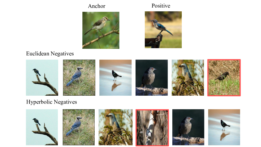
Figure 1: For a random chosen anchor, we arrange hard negatives selected by a well-trained model based on their distance to the anchor. The top row displays the anchor and its positive pair. We present sorted negatives from Euclidean embedding model (“Sph-ViT") and the hyperbolic embedding model (“Hyp-ViT"), respectively. Negatives are ordered by increasing distance from left to right. “Sph-ViT" is trained with $\tau=0.05$, while “Hyp-ViT" is trained with $\tau=0.05$ and $c=0.1$. Red boxes highlight negatives that are absent in the top 6 hard negatives of the other model.

Pair-wise losses including contrastive loss [34], triplet loss [119], N-pair loss [98], and InfoNCE [75, 14] are fundamental in metric learning, constructed based on instance relationships within a batch. Contrastive loss, for instance, treats views of data from the same class as positive pairs and other batch data as negative pairs, encouraging the encoder to map positive pairs close and negative pairs apart. Contrastive learning embeddings are positioned on a hypersphere using the inner product as a distance measure [16]. However, fields like social networks, brain imaging, and computer graphics often exhibit hierarchical structures [6].

A recent trend in representation learning is using hyperbolic spaces, which excel in capturing hierarchical data [78]. Unlike Euclidean space with polynomial volume growth, hyperbolic space demonstrates exponential growth suitable for tree-like data structures. Hyperbolic representations have shown success in NLP [72, 73], image segmentation [121, 3], few-shot [49] and zero-shot learning [63], as well as representation learning and metric learning [25, 29, 128, 62, 61]. In hyperbolic space, feature similarity is calculated via distance measurement after projecting data features.

Motivation. While hyperbolic contrastive loss is effective in metric learning, the underlying reason has yet to be fully understood. Prior research has demonstrated that employing a vision transformer-based model for metric learning with output embeddings mapped to hyperbolic space outperforms Euclidean embeddings [25]. Nonetheless, our experimental findings indicate that a straightforward embedding approach in one geometry doesn’t consistently yield superior results compared to the other. The choice of temperature parameter ($\tau$) in the loss function and the curvature values in hyperbolic space contribute to the performance variations among different embeddings. Moreover, Euclidean and hyperbolic embeddings exhibit complementary behavior with diverse $\tau$ and curvature values. As depicted in Fig. 1, embedding features under different geometries occasionally highlight different crucial instances. This observation sparks our interest in delving further into hyperbolic metric learning.

The pair-wise contrastive loss relies on two key components: positive pairs $(\mathbf{x},\mathbf{x}^{+})$, and negative pairs $(\mathbf{x},\mathbf{x}^{-})$ of data. The strategies of positive sampling has been studied intensively [5, 126, 4, 14, 108, 18, 107, 100, 65, 75, 80, 92], as well as the negative data augmentation e.g., [48, 30, 85, 95] where most of the works focus on “hard” negative data augmentation. For instance, [85] provided a popular principle that “The most useful negative samples are ones that the embedding currently believes to be similar to the anchor”, where the embedding refers to the network output. That is, letting $\mathbf{x}_{1}^{-},\mathbf{x}_{2}^{-}$ be two negative samples w.r.t. the anchor $\mathbf{x}$ and $\phi$ be the current network, then $x_{1}^{-}$ is more useful (i.e., harder) than $\mathbf{x}_{2}^{-}$ if $\phi(\mathbf{x})^{T}\phi(\mathbf{x}_{1}^{-})>\phi(\mathbf{x})^{T}\phi(\mathbf{x}_{2}^{-})$ holds, where $(\cdot)^{T}$ denotes the matrix transpose operator.

Our analysis reveals that the differences in embedding performance stem from the distinct effects of hard negative sampling in the two geometries. This analysis shifts our focus from individual hard negative instances to hard triplets. We demonstrate that triplet selection hinges on a weight $p(\mathbf{x}^{-})$, which varies across different geometries for the same instance. To capitalize on the benefits of these diverse geometries, we introduce the concept of embedding fusion. Our solution is driven by two essential insights: 1) different geometries yield variety in hard negative selection properties, and 2) distinct geometries complement each other in triplet selection.

In contrast to prior studies that emphasize selecting more meaningful negative samples [20, 84, 114, 48, 130, 40, 93, 30], our primary contribution lies in understanding the performance disparity across different geometries. Our experiments unveil the complementary performance of diverse geometries. We delve into unexplored aspects of hyperbolic metric learning through an analysis of hard triplet selection. Furthermore, we present a direct solution for effectively utilizing information from different geometries. Demonstrating the efficacy of our straightforward fusion algorithm, we adhere to the standard design of vision transformer-based metric learning. By adopting an ensemble approach, our model effectively captures more informative negative samples from an additional pool, resulting in enhanced performance.

2 Related Work

Hyperbolic Embeddings. The machine learning community has a long history of embracing Euclidean space for representation learning. It is a natural generalization of our intuition-friendly, physically-accessible three-dimensional space where the measurable distance is represented with inner-product [27, 78]. However, the Euclidean embedding may not best fit in some complex tree-like data fields such as Biology, Network Science, Computer Graphics, or Computer Vision that exhibit highly non-Euclidean latent geometry [27, 6].

In the computer vision domain, the hyperbolic space has been found well-suited for image segmentation [121, 3], zero-shot recognition [63, 26], few-shot image classification [49, 26, 28] as well as point cloud classification [69]. The work of [33] revealed the vanishing gradients issue of Hyperbolic Neural Networks (HNNs) when applied to classification benchmarks that may not exhibit hierarchies and showed clipped HNNs are more robust to adversarial attacks. Concurrently, [25, 128, 29] mapped the output-of-image representations encoded by a backbone to a hyperbolic space to group the representations of similar objects in the embedding space. They empirically verified the performance of pairwise cross-entropy loss with the hyperbolic distance in image embeddings while we investigate the reason why contrastive metric learning works in hyperbolic space and when the method will work without hyperbolic embedding.

Pair-wise Losses. One of the fundamental losses in metric learning is contrastive loss [34]. The contrastive representation learning attempts to pull the embeddings of positive pairs closer and push the embeddings of negative pairs away in the latent space by optimizing the pair-wise objective. Following these fundamental concepts, many variants have since been proposed, such as triplet margin loss [119], angular loss [115], margin loss [122], etc. Other losses contain softmax operation and LogSumExp for a smooth approximation of the maximum function. For example, the lifted structure loss [74] applies LogSumExp to all negative pairs, and the N-Pairs loss [98] applies the softmax function to each positive pair relative to all other pairs. Recently, learning representations from unlabeled data in contrastive way [19, 34] has been one of the most competitive research field [75, 38, 124, 107, 98, 14, 44, 57, 36, 18, 15, 4, 68, 11]. Popular model structures like SimCLR [14] and Moco [36] apply the commonly used loss function InfoNCE [75] to learn a latent representation that is beneficial to downstream tasks. Several theoretical studies show that self-supervised contrastive loss optimizes data representations by aligning positive pairs while pushing negative pairs away on the hypersphere [116, 16, 114, 2]. Recently, the loss has been applied in metric learning and shows superior performance when equipped with ViT and hyperbolic embedding.

Hard-negative Mining. When applying contrastive loss, the positive pairs could be different modalities of a signal [1, 107, 110], different data augmentations of the same image, e.g., color distortion, random crop [14, 18, 32] or instances from the same category like in image retrieval. [108] suggested generating the positive pairs with “InfoMin principle" so that the generated positive pairs maintain the minimal information necessary for the downstream tasks. [91, 79, 67, 59] proposed selecting meaningful but not fully overlapped contrastive crops with guidance like attention maps or object-scene relations. [94] empirically demonstrated that introducing extra convex combinations of data as positive augmentation improves representation learning. Similar mixing data strategies could be found in [55, 51, 113, 56, 83]. Other than exploring positive augmentation, recent works focus on negative data selection in contrastive learning. Typically, negative samples are drawn uniformly from the training data. Based on the argument that not all negatives are true negatives, [20, 84] developed debiased contrastive loss to assign higher weights to the hard negative samples. [114] proposed an explicit way to select the hard negative samples similar to the positive. To provide more meaningful negative samples, [48] studied the Mixup [130] strategy in latent space to generate hard negatives. [40] proposed directly learning a set of negative adversaries. [30] generated negative samples by texture synthesis or selecting non-semantic patches from existing images. Unlike previous studies, we do not propose a new method for negative data sampling but provide some insights on the real “hard” negatives from the perspective of the gradients of contrastive loss. We try to understand when data are embedded in different spaces, which factor contributes to the “good” embeddings. Based on our analysis, we propose to learn embeddings under a mixture of geometries.

3 Understanding Geometry Effect

We introduce the relevant preliminaries, such as hyperbolic geometry and pairwise cross-entropy used in metric learning, in Section 3.1. The relationship between geometries and triplet selection is analyzed in Section 3.2. In Section 3.3, we present embedding fusion as a strategy to utilize complementary information from diverse geometries, accompanied by discussing the distinctions between our approach and existing hard negative sampling methods.

3.1 Preliminaries

Among several isometric models [9] of hyperbolic space, we stick to the Poincaré ball model [88] that is well-suited for gradient-based optimization (i.e., the distance function is differentiable). In particular, the model $(\mathbb{M}^{n}_{c},g^{\mathbb{M}})$ is defined by the manifold $\mathbb{M}^{n}=\{x\in\mathbb{R}^{n}\colon c\|x\|^{2}<1,c\geq 0\}$ equipped with the Riemannian metric $g^{\mathbb{M}}=\lambda_{c}^{2}g^{E}$, where $c$ is the curvature parameter and $\lambda_{c}=\frac{2}{1-c\|x\|^{2}}$ is conformal factor that scales the local distances. $g^{E}=\mathbf{I}_{n}$ denotes the Euclidean metric tensor.

The framework of gyrovector spaces provides an elegant non-associative algebraic formalism for hyperbolic geometry just as vector spaces provide the algebraic setting for Euclidean geometry [9, 111, 112, 27]. For two vectors $\mathbf{x},\mathbf{y}\in\mathbb{M}^{n}_{c}$, their addition is defined as

$$\small\mathbf{x}\oplus_{c}\mathbf{y}=\frac{(1+2c\langle\mathbf{x},\mathbf{y}\rangle+c\|\mathbf{y}\|^{2})\mathbf{x}+(1-c\|\mathbf{x}\|^{2})\mathbf{y}}{1+2c\langle\mathbf{x},\mathbf{y}\rangle+c^{2}\|\mathbf{x}\|^{2}\|\mathbf{y}\|^{2}}.$$ (1)

The hyperbolic distance between $\mathbf{x},\mathbf{y}\in\mathbb{M}^{n}_{c}$ is defined as:

$$\small D_{hyp}(\mathbf{x},\mathbf{y})=\frac{2}{\sqrt{c}}\mathrm{arctanh}(\sqrt{c}\|-\mathbf{x}\oplus_{c}\mathbf{y}\|).$$ (2)

In particular, when $c=0$, the Eq. 1 is the Euclidean addition of two vectors in $\mathbb{R}^{n}$ and Eq. 2 recovers Euclidean geometry: $\lim_{c\to 0}D_{hyp}(\mathbf{x},\mathbf{y})=2\|\mathbf{x}-\mathbf{y}\|.$ For an open $n$-dimensional unit ball, the geodesics of the Poincaré disk are then circles that are orthogonal to the boundary of the ball.

Before performing operations in the hyperbolic space, a map termed exponential is used when mapping from Euclidean space to the Poincaré model of hyperbolic geometry [49]. The exponential map is defined as:

$$\small\exp_{\mathbf{x}}^{c}(\mathbf{v})=\mathbf{x}\oplus_{c}\bigg{(}\tanh\bigg{(}\sqrt{c}\frac{\lambda_{\mathbf{x}}^{c}\|\mathbf{v}\|}{2}\bigg{)}\frac{\mathbf{v}}{\sqrt{c}\|\mathbf{v}\|}\bigg{)}$$ (3)

In practice, we follow the setting of [49] and [25] with the base point $\mathbf{x}=\mathbf{0}$ so that the formulas are less cumbersome and empirically have little impact on the obtained results.

For metric learning method, we adapt the approach suggested by [25], each iteration involves sampling two data points, $(\mathbf{x},\mathbf{x}^{+})$, from $N$ distinct image categories to form positive pairs. All the other data in the same batch construct negative pairs with the anchor $(\mathbf{x},\mathbf{x}^{-})$. In this case, the total number of samples (batch size) is $K=2N$ consisting of $N$ positive pairs.

Pairwise Cross-Entropy Loss. Self-supervised contrastive learning, such as [14, 106, 38], employs the following InfoNCE loss to attract positive pairs and separate negatives from the anchor in the latent space.

$$\small\mathcal{L}_{NCE}=-\sum_{i\in I}\log{\frac{\text{exp}\left(s_{i,i}/\tau\right)}{\text{exp}\left(s_{i,i}/\tau\right)+\sum_{k\neq i}\text{exp}\left(s_{i,k}/\tau\right)}}$$ (4)

In this context, $(i,i)$ refers to the anchor and its positive pair, and the other $2(N-1)$ indices denote the anchor’s negatives. For each anchor $i$, there exists $1$ positive pair and $2N-2$ negative pairs. The denominator comprises a total of $2N-1$ terms. $\tau\in\mathcal{R}^{+}$ is the scalar temperature parameter that governs sharpness, $s_{i,j}=\mathbf{z}_{i}\cdot\mathbf{z}_{j}$ with $\mathbf{z}=g(f(\mathbf{x}))$. $f(\cdot)$ maps $\mathbf{x}$ to lower dimension using a shared ViT architecture [22]. $g(\cdot)$ projects $f(\mathbf{x})$ to latent space. Typically, $\mathbf{z}$ is normalized before loss calculation to lie on a unit hypersphere.

$$\small D_{cos}(\mathbf{z}_{i},\mathbf{z}_{j})=\left\lVert\frac{\mathbf{z}_{i}}{\left\lVert\mathbf{z}_{i}\right\rVert_{2}}-\frac{\mathbf{z}_{j}}{\left\lVert\mathbf{z}_{j}\right\rVert_{2}}\right\rVert^{2}_{2}=2-2\frac{\mathbf{z}_{i}\cdot\mathbf{z}_{j}}{\left\lVert\mathbf{z}_{i}\right\rVert_{2}\cdot\left\lVert\mathbf{z}_{j}\right\rVert_{2}}$$ (5)

The general loss form of pairwise cross-entropy loss in Euclidean and hyperbolic space is defined as

where $D_{i,j}$ is the distance measurement like $D_{cos}(\mathbf{z}_{i},\mathbf{z}_{j})$ or $D_{hyp}(\mathbf{z}_{i},\mathbf{z}_{j})$.

3.2 Geometries vs. Hard Negatives

In this study, we investigate the conditions under which contrastive loss yields superior performance across distinct geometries. Fig. 2 presents the performance comparison of ViT models trained with varying temperature values ($\tau$) and curvature parameter ($c$). “Sph-” are versions with Euclidean ($c=0$) embeddings optimized using $D_{cos}$ (5). “Hyp-” are versions with hyperbolic embeddings optimized using $D_{hyp}$ (2). Hyperbolic embeddings generally enhances performance, especially when $\tau\geq 0.2$ as shown in Fig. 2. From a hyperbolic geometry perspective, in hyperbolic space, the distance between a point and the origin experiences exponential growth. When comparing two points, the relative distance between them becomes larger in hyperbolic space due to this exponential distance growth. In the following analysis, we will demonstrate how this geometry impacts negative selection.

Our analysis is supported by empirical experiments utilizing the current state-of-the-art approach in metric learning for image retrieval. Through gradient analysis of the InfoNCE loss in Euclidean space, followed by its generalization to hyperbolic geometry, we reveal the substantial impact of various geometries on the triplet selection weights $(\mathbf{x},\mathbf{x}^{+},\mathbf{x}^{-})$.

Specifically, $\mathcal{L}_{NCE}$ could be further rewritten as

$$\small\begin{split}\mathcal{L}_{NCE}&=\sum_{i\in I}\log\left({1+\frac{\sum_{k\neq i}\text{exp}\left(s_{i,k}/\tau\right)}{\text{exp}\left(s_{i,i}/\tau\right)}}\right)\\ &=\sum_{i\in I}\log\left(1+\sum_{k\neq i}\text{exp}\left(\frac{1}{\tau}\left(s_{i,k}-s_{i,i}\right)\right)\right).\end{split}$$ (7)

The gradient is derived as: $\nabla\mathcal{L}_{NCE}=\sum_{i\in I}\nabla\mathcal{L}_{i}$ where

$$\small\nabla\mathcal{L}_{NCE_{i}}=\frac{1}{\tau}\sum_{k\neq i}p(\mathbf{x}^{-})\nabla\left(s_{i,k}-s_{i,i}\right)$$ (8)

with $p(\mathbf{x}^{-})=\frac{\text{exp}\left(s_{i,k}/\tau\right)}{\text{exp}\left(s_{i,i}/\tau\right)+\sum_{k\neq i}\text{exp}\left(s_{i,k}/\tau\right)}\in[0,1]$. Detailed derivations are presented in the supplementary material.

Then stochastic gradient descent (SGD) can be used to update network weights. As for the general gradient form that includes hyperbolic space, it is just

$$\small\nabla\mathcal{L}_{hyp_{i}}=\frac{1}{\tau}\sum_{k\neq i}p(\mathbf{x}^{-})\nabla\left(D_{i,i}-D_{i,k}\right)$$ (9)

with $p(\mathbf{x}^{-})=\frac{\text{exp}\left(-D_{i,k}/\tau\right)}{\text{exp}\left(-D_{i,i}/\tau\right)+\sum_{k\neq i}\text{exp}\left(-D_{i,k}/\tau\right)}\in[0,1]$.

The gradient analysis shows that each $p(\mathbf{x}^{-})$ decides the weights contributed by each triplet $(\mathbf{x},\mathbf{x}^{+},\mathbf{x}^{-})$ to the gradient update. $p(\mathbf{x}^{-})$ is further related to the relative distance between positve pair and negative pairs. By looking into the term $p(\mathbf{x}^{-})$ we get the following conclusions:

• $p(\mathbf{x}^{-})$ is non-uniform for all triplet selection. Temperature parameter $\tau$ plays an important role in deciding the weights of gradient update for each negative pair. $p(\mathbf{x}^{-})$ is larger with smaller $\tau$.

• The relative distance between $(\mathbf{x},\mathbf{x}^{+})$ and $(\mathbf{x},\mathbf{x}^{-})$ decides the gradient contribution by a negative instance.

• For the same $\tau$, when we change from Euclidean distance to hyperbolic distance (varying $c$), the relative distance between a negative pair and a positive pair will be enlarged due to the geometry property of hyperbolic space. This will further affect the hard negative sampling.

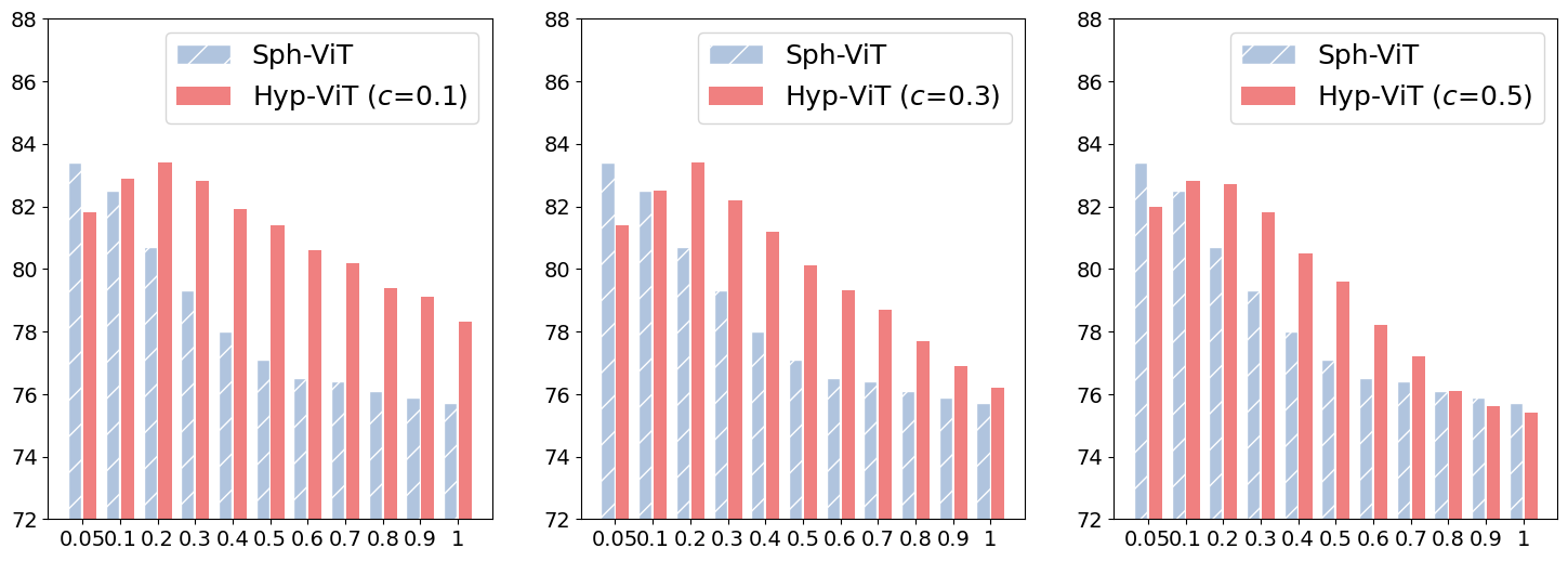
Figure 2: Experimentally, we find that Euclidean (“Sph”) and hyperbolic (“Hyp”) embeddings, with varying $\tau$ and $c$ values, exhibit complementary characteristics which is attributed to differences in negative selection across distinct geometry embeddings. To leverage this complementary information from different geometries, we introduce embedding fusion.

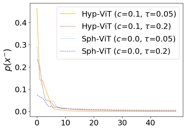
Figure 3: $p(\mathbf{x}^{-})$ for different ViT. x-axis is the index of data points when the distance between $(\mathbf{x}^{-})$ to anchor point $\mathbf{x}$ is sorted in ascending order (better view in color print).

3.3 Ensemble Learner with Mix Geometries

We empirically verify the above analysis with the method proposed by [25]. We follow the exact experiment settings proposed by previous work. The detail of the experiments can be found in the following section.

As asserted by [25], optimizing pairwise contrastive loss in hyperbolic space yields a new state-of-the-art performance surpassing Euclidean embeddings. In their study, they set $\tau=0.1$ for Euclidean space and $\tau=0.2$ for hyperbolic space, with a curvature parameter of $c=0.1$. Interestingly, upon conducting similar experiments with varying $\tau$ from a small value of $0.05$ to $1$, we observe that proper tuning of $\tau$ can lead to optimal performance in Euclidean space embeddings as well. Both Euclidean and hyperbolic embeddings exhibit performance drops with larger $\tau$ values. This trend is consistent across different backbone encoders, as illustrated in the supplemental material. The impact of $\tau$ relates to $p(\mathbf{x}^{-})$ in Eq. 11 and Eq. 9, where smaller $\tau$ assigns higher weights to harder negatives (i.e., negative samples $\mathbf{x}^{-}$ that are closer to the anchor $\mathbf{x}$ than the positive sample $\mathbf{x}^{+}$).

We empirically validate our analysis of $p(\mathbf{x}^{-})$ by visualizing a small batch $\mathbf{x}^{-}$ after the model converges (Fig. 3). The horizontal axis represents data point indices, sorted based on their distance from the anchor point. We present the results for two sets of temperature values: $\tau=0.05$ for Euclidean embeddings and $\tau=0.2$ for hyperbolic embeddings, corresponding to their respective optimal performance points. Notably, at $\tau=0.05$, the weights $p(\mathbf{x}^{-})$ for hard negatives can reach as high as 0.46, compared to Euclidean embeddings. Similarly, at $\tau=0.2$, instances closer to the anchor exhibit significantly higher $p(\mathbf{x}^{-})$ than in Euclidean embeddings. This observation confirms the non-uniform distribution of $p(\mathbf{x}^{-})$. Among all available triplet combinations ($\mathbf{x},\mathbf{x}^{+},\mathbf{x}^{-}$), the majority exhibit small $p(\mathbf{x}^{-})$ values, while a small portion has relatively larger values. It is these selected triplets that significantly contribute to shaping the decision boundary. The process of selecting important triplets is greatly influenced by $p(\mathbf{x}^{-})$, which plays a crucial role. Different geometries lead to distinct feature selections, guided by the variations in $p(\mathbf{x}^{-})$.

Motivated by our observation of complementary performance across different geometries, the idea of fusing their features to harness this complementary information arises naturally. In Fig. 1, we illustrate the hard negatives selected by well-trained models embedded in different geometries, based on their distances to the anchor. The distinct triplet pools selected by these embeddings are evident. For the same instance, $p(\mathbf{x}^{-})$ varies between Euclidean and hyperbolic embeddings. If both $p(\mathbf{x}^{-})$ values are small, the instance doesn’t significantly contribute to the decision boundary. If one value is high, it will be considered if selected from the fusion pool.

Learning with Mixed Geometries. As our analysis indicates, within each embedding space, the model effectively selects hard negative samples for proficient representation learning. Fusion empowers the model to choose from the amalgamated triplet pool. Two direct approaches exist for constructing the ensemble learner. One involves a convex combination of loss functions from two distinct geometries, such as $\lambda\mathcal{L}_{hyp}+(1-\lambda)\mathcal{L}_{NCE}$. Yet, our experimental tests indicated that this form did not yield improved results. Consequently, we adopt the second approach, which involves feature space fusion. Our proposed $\mathcal{L}_{mix}$ is defined as

where $\lambda$ is a tunable hyperparameter that controls the hard negative selecting effect from different geometries.

Comparing with Hard Negative Sampling Methods. Recent studies have concentrated on negative data selection within contrastive learning. Notably, [20, 84] introduced debiased contrastive loss to assign higher weights to challenging negative samples. Alternatively, [114] proposed an explicit strategy for selecting hard negative samples that resemble positives. To enhance the relevance of negative samples, [48] explored Mixup [130] in the latent space to generate challenging negatives. [40] directly learned negative adversaries, while [93] proposed negative selection through quadratic optimization, and [30] generated negatives via texture synthesis or non-semantic patches.

Diverging from previous works, our study comprehends hyperbolic geometry through the lens of triplet selection. We do not solely aim to enhance contrastive learning via hard negative sampling. Rather, we scrutinize the assertion that hyperbolic embeddings consistently outperform Euclidean embeddings, as shown in earlier studies. Our analysis reveals that triplet selection varies across geometries. From this perspective, we propose that combining different geometries can expand the sampling pool. Our experiments demonstrate that mixed geometries prompt the model to select triplets crucial to the decision boundary, while discarding less significant ones present in both embeddings. A potential future direction could be merging existing negative sampling methods with different geometries.

Method	CUB-200-2011 (K)				Cars-196 (K)				SOP (K)
	1	2	4	8	1	2	4	8	1	10	100	1000
Margin [123]	63.9	75.3	84.4	90.6	79.6	86.5	91.9	95.1	72.7	86.2	93.8	98.0
FastAP [8]	-	-	-	-	-	-	-	-	73.8	88.0	94.9	98.3
NSoftmax [129]	56.5	69.6	79.9	87.6	81.6	88.7	93.4	96.3	75.2	88.7	95.2	-
MIC [86]	66.1	76.8	85.6	-	82.6	89.1	93.2	-	77.2	89.4	94.6	-
XBM [118]	-	-	-	-	-	-	-	-	80.6	91.6	96.2	98.7
IRTR [24]	72.6	81.9	88.7	92.8	-	-	-	-	83.4	93.0	97.0	99.0
Sph-DINO	77.9	86.1	91.6	95.1	82.5	89.2	93.3	95.8	84.6	94.2	97.6	99.2
Sph-ViT $\mathsection$	83.4	90.2	94.0	96.3	78.8	86.7	91.9	95.0	85.5	94.9	98.2	99.5
Hyp-DINO	78.3	86.8	92.0	95.4	83.2	90.0	93.8	96.3	84.0	93.9	97.6	99.2
Hyp-ViT $\mathsection$	83.4	90.2	94.2	96.3	80.1	88.1	92.8	95.7	85.3	94.8	98.1	99.5
Mix-DINO	78.5	86.9	91.8	95.3	85.2	91.2	94.6	96.8	84.9	94.3	97.7	99.3
Mix-ViT $\mathsection$	83.7	90.4	94.1	96.5	81.3	88.5	93.2	96.1	85.8	95.0	98.1	99.5

Table 1: Recall@K for three datasets for 128-dimensional embeddings. Our methods are listed in the last two rows, evaluated for head embeddings. “Sph-” and “Hyp-” indicate hypersphere embeddings optimised using $D_{cos}$ (5) and hyperbolic embeddings optimised using $D_{hyp}$ (2), respectively. “DINO” and “ViT” are types of pretraining vision transformer encoder. Models shown at the top are based on ResNet-50 [37] encoder, except IRT_R is based on DeiT [109]. In our method, we take $\lambda$ value 3 for CUB, and 8 for Cars and SOP.                                                                                                                                                                        ^{$\mathsection$} pretrained on the larger ImageNet-21k [21]. The best results, within a non-significant difference of 0.1, are highlighted.

Method	Dim	CUB-200-2011 (K)				Cars-196 (K)				SOP (K)
		1	2	4	8	1	2	4	8	1	10	100	1000
A-BIER [76]	512	57.5	68.7	78.3	86.2	82.0	89.0	93.2	96.1	74.2	86.9	94.0	97.8
ABE [52]	512	60.6	71.5	79.8	87.4	85.2	90.5	94.0	96.1	76.3	88.4	94.8	98.2
SM [102]	512	56.0	68.3	78.2	86.3	83.4	89.9	93.9	96.5	75.3	87.5	93.7	97.4
XBM [118]	512	65.8	75.9	84.0	89.9	82.0	88.7	93.1	96.1	79.5	90.8	96.1	98.7
HTL [31]	512	57.1	68.8	78.7	86.5	81.4	88.0	92.7	95.7	74.8	88.3	94.8	98.4
MS [117]	512	65.7	77.0	86.3	91.2	84.1	90.4	94.0	96.5	78.2	90.5	96.0	98.7
SoftTriple [81]	512	65.4	76.4	84.5	90.4	84.5	90.7	94.5	96.9	78.6	86.6	91.8	95.4
HORDE [43]	512	66.8	77.4	85.1	91.0	86.2	91.9	95.1	97.2	80.1	91.3	96.2	98.7
Proxy-Anchor [50]	512	68.4	79.2	86.8	91.6	86.1	91.7	95.0	97.3	79.1	90.8	96.2	98.7
NSoftmax [129]	512	61.3	73.9	83.5	90.0	84.2	90.4	94.4	96.9	78.2	90.6	96.2	-
ProxyNCA++ [105]	512	69.0	79.8	87.3	92.7	86.5	92.5	95.7	97.7	80.7	92.0	96.7	98.9
IRTR [24]	384	76.6	85.0	91.1	94.3	-	-	-	-	84.2	93.7	97.3	99.1
ResNet-50 [37] †	2048	41.2	53.8	66.3	77.5	41.4	53.6	66.1	76.6	50.6	66.7	80.7	93.0
DeiT-S [109] †	384	70.6	81.3	88.7	93.5	52.8	65.1	76.2	85.3	58.3	73.9	85.9	95.4
DINO [12] †	384	70.8	81.1	88.8	93.5	42.9	53.9	64.2	74.4	63.4	78.1	88.3	96.0
ViT-S [101] † $\mathsection$	384	83.1	90.4	94.4	96.5	47.8	60.2	72.2	82.6	62.1	77.7	89.0	96.8
Sph-DINO	384	80.5	87.9	92.5	95.4	87.0	92.7	95.9	97.6	84.8	94.2	97.6	99.2
Sph-ViT $\mathsection$	384	85.1	91.1	94.3	96.5	82.2	89.0	93.3	96.2	85.3	94.5	97.9	99.4
Hyp-DINO	384	80.6	88.1	92.8	95.4	87.5	93.1	96.2	97.9	84.5	94.1	97.6	99.2
Hyp-ViT $\mathsection$	384	85.0	91.3	94.5	96.5	84.3	90.8	94.8	97.3	85.2	94.6	98.0	99.4
Mix-DINO	384	80.4	88.3	92.8	95.5	88.9	94.1	96.5	98.1	85.1	94.5	97.8	99.3
Mix-ViT $\mathsection$	384	84.6	91.3	94.9	96.7	84.4	90.6	94.9	97.1	86.0	95.0	98.2	99.5

Table 2: Recall@K metric for three datasets, “Dim” column shows the dimensionality of embeddings. The 2 versions of our method are listed in the bottom section starting with “Mix”, evaluated for encoder embeddings. Encoders by methods: A-BIER, ABE, SM: GoogleNet [104]; XBM, HTL, MS, SoftTriple, HORDE, Proxy-Anchor: Inception with batch normalization [42]; NSoftmax, ProxyNCA++: ResNet-50 [37]; IRT_R: DeiT [109]. ^† pretrained encoders without training on the target dataset. ^{$\mathsection$} pretrained on the larger ImageNet-21k [21]. The best results and the second best, within a difference of 0.1, are highlighted.

4 Experiments and Results

We adhere to the training and evaluation protocol established by [25]. We then contrast two versions of our approach with the current state-of-the-art across three benchmark datasets for image retrieval tasks. In the upcoming sections, we introduce the datasets and contrastive methods in Section 4.1, provide implementation specifics in Section 4.2, and present the experimental results in Section 4.3.

4.1 Datasets

We perform the evaluation of our method on three different benchmark datasets. CUB-200-2011 (CUB) [120] includes 11,788 images with 200 categories of bird breeds. We use the first 100 classes with 5,864 images as the training set, and the remaining 100 classes with 5,924 images are used for testing. The instance in this dataset is hard to distinguish visually. Some breeds could only be distinguished by minor details, making this dataset challenging and, at the same time, informative for the image retrieval task. Cars-196 (Cars) [54] is a dataset containing 16,185 images of 196 car models. The first 98 classes (8,054 images) are used for training and the other 98 classes (8,131 images) are used for testing. Stanford Online Product (SOP) [99] consists of 120,053 images of 22,634 products downloaded from eBay.com. We follow the standard train/test split: 11,318 classes (59,551 images) for training and the remaining 11,316 classes (60,502 images) for testing.

4.2 Implementation Details

We adopt the code implementation and hyper-parameter of [25]. For the pretrained backbone encoders, we use ViT-S [101] with two different types of pretraining (ViT-S and DINO). The ViT architecture was introduced by [23]. The input image is cut into patches of size $16\times 16$. Each patch is flattened and then linearly projected into an embedding as well as their location information. ViT-S [101] is the smaller version of ViT with 6 heads in multiheaded self-attention (base version uses 12 heads). A detailed description is available in [101]. We use the publicly available version of ViT-S pretrained on ImageNet-21k [101]. The second encoder used in our experiments is DINO [12], which is an architecture proposed for contrastive self-supervised representation learning. In this configuration, the model ViT-S is trained on the ImageNet-1k dataset [87] without labels. Detailed architecture design could be found in [12].

We replicate the experiment design and implementation details from previous work. Head biases are initialized to $0$, and weights with a (semi) orthogonal matrix [89]. In fine-tuning, linear projection for patch embeddings remains frozen. The encoder yields a $384$-dimensional representation, projected by a head to a $128$-dimensional space. The model has two branches: one outputs a $128$-dimensional embedding in Euclidean space, while the other projects into hyperbolic space. Our proposed method for feature mixtures across geometries is then applied. Notably, encoder outputs are normalized prior to branching. Following [25], we adopt naming conventions: the hyperbolic head baseline is “Hyp-”, and the unit hypersphere is “Sph-”.

Hyperbolic space consistently follows a trend when adjusting curvature parameter $c$ from small to large values. Optimal performance is achieved at $\tau=0.2$ then gradually declines. For smaller $c$ values, hyperbolic embeddings outperform Euclidean embeddings when $\tau>0.2$. In our mixture model, we utilize $c=0.1$ and $\tau=0.2$ for hyperbolic embeddings, and $\tau=0.05$ for hypersphere embeddings. Lambda is tested from $1$ to $10$ to determine the best value. The clipping radius remains consistent with previous work at $r=2.3$.

We use the AdamW optimizer [66] with a learning rate value $1\times 10^{-5}$ for DINO and $3\times 10^{-5}$ for ViT-S. The weight decay value is $0.01$, and the batch size equals $900$. The number of optimizer steps depends on the dataset: $200$ for CUB, $600$ for Cars, $25000$ for SOP. The gradient is clipped by norm $3$ for greater stability. We apply commonly used data augmentations: random crop resizing the image to $224\times 224$ using bicubic interpolation combined with a random horizontal flip. We implemented the automatic mixed precision training with Pytorch [77]. All experiments are performed on one NVIDIA A100 80G GPU.

For the baseline method proposed in [25], we re-implemented the code and report the results run by ourselves.

4.3 Results

Tab. 1 and Tab. 2 report the experimental recall@K metric for the 128-dimensional head embedding and the results for 384-dimensional encoder embedding. The evaluation results of the pretrained encoders without training on the target dataset in Tab. 2 are from [25]. The last 6 rows in the tables present the results obtained from our implementation.

In Fig. 2, it is shown that the performance of Euclidean embedding is governed by temperature parameter $\tau$. The smallee the temperature is, the better the performance. On the other hand, the performance of hyperbolic embedding is dominated by the choice of both $\tau$ and $c$. Different $c$ values will assign different relative distances between samples. Unlike the Euclidean embedding, most hyperbolic embedding shows better performance when $\tau$ is around 0.2. Different embeddings will give supplementary features to each other.

The observations from Fig.2, Tab.1, and Tab. 2 demonstrate that the Euclidean embedding model performs comparably, and sometimes even better, than the hyperbolic embedding method when the temperature parameter is small ($\tau=0.05$). This aligns with our analysis that Euclidean space provides sufficient embeddings as long as the temperature $\tau$ effectively promotes meaningful hard negative selection. Existing work lacks a comprehensive Euclidean vs. hyperbolic space comparison concerning temperature effects in the contrastive loss, leading to potentially inflated performance claims for hyperbolic embeddings.

For 128-dimensional embeddings, our Mix model achieves the best 1K recall value, outperforming Sph and Hyp baselines, even after their optimal tuning. In the CUB dataset, recall improvements for 1K, 2K, and 8K are 0.36%, 0.22%, and 0.21%, respectively. In the Cars dataset, DINO consistently outperforms ViT, allowing our Mix method to also excel when using DINO as the backbone encoder. The relative improvements for 1K, 2K, 4K, and 8K are 2.40%, 1.33%, 0.85%, and 0.52%, respectively. Similarly, for SOP, there are relative improvements of 0.35% and 0.11% in 1K and 10K recall, respectively.

For 384-dimensional embeddings, our proposed Mix model shows promise. In the CUB dataset, 1K recall is slightly lower than the Sph-ViT method. Notably, on CUB, relative performance improvements for 4K and 8K are 0.42% and 0.21%, respectively. For the Cars dataset, relative improvements in 1K, 2K, 4K, and 8K recall are 1.60%, 1.07%, 0.31%, and 0.20%, respectively. In the SOP dataset, the relative improvements for 1K, 10K, 100K, and 1000K recall are 0.82%, 0.42%, 0.20%, and 0.10%, respectively. The experiments were conducted multiple times, with standard deviations around 0.2.

In our analysis in Section 3.3, we demonstrate that the value of $p(\mathbf{x}^{-})$ varies between Euclidean and hyperbolic embeddings for the same instance. This discrepancy implies that the models will exhibit different preferences when selecting the corresponding triplet $(\mathbf{x},\mathbf{x}^{+},\mathbf{x}^{-})$ to learn decision boundaries. We hypothesize that mixed geometry embeddings may not consistently outperform single geometry embeddings to a significant extent. In some cases, their performance could be comparable to that of single geometry embeddings. This is due to the fact that the selection of negatives in each geometry is determined by $p(\mathbf{x}^{-})$. Instances with low values of $p(\mathbf{x}^{-})$ in both geometries have minimal impact on the decision boundary. On the other hand, instances with high $p(\mathbf{x}^{-})$ in one geometry but low in the other might be overlooked by one embedding, yet highlighted when the corresponding $p(\mathbf{x}^{-})$ remains high after fusion. However, it’s not guaranteed that the mixed model will always put emphasis on true hard negatives when learn a model. Our proposed method aims to validate our understanding of different geometry embeddings, rather than proposing an explicit negative selection method. This explains why the mixed model occasionally surpasses single-geometry embeddings but not consistently.

In our proposed method, we only tested simple addition as feature fusion. However, considering different $c$ values will result in new hyperbolic geometries, and further gains are possible if more embedding spaces are considered in the proposed Mix model.

5 Conclusion

Upon scrutinizing recent advancements in metric learning employing hyperbolic space, we uncover that the performance boost attributed to hyperbolic space primarily arises from parameter tuning of $\tau$ in the pairwise cross-entropy loss. Experimentally, we find Euclidean and hyperbolic embeddings exhibit complementary behavior with diverse $\tau$ and curvature values. This observation motivates us to delve deeper into hyperbolic metric learning. Our analysis reveals that the distinct performance of embeddings stems from varying effects of hard negative sampling in the two geometries, illustrated in Fig. 1. To harness the benefits of these diverse geometries, we propose an ensemble learning approach that amalgamates features acquired in two spaces. By altering the hard negative data pool during the learning process, we encourage the model to acquire more informative features.

Limitation. In our current fusion experiment, we determine the optimal $\lambda$ value through a uniform search spanning 1 to 10. For future endeavors, an automated approach, such as incorporating $\lambda$ as a learnable parameter, could be explored. Additionally, our fusion model currently involves a simple convex combination of Euclidean and hyperbolic geometry. Considering the varying nature of hyperbolic geometry with changes in $c$, the fusion model’s scope could potentially encompass more than two geometries. We believe this work offers insightful contributions to comprehending hyperbolic metric learning. Furthermore, the exploration and analysis of potential ensemble learning involving Euclidean and hyperbolic geometry in different configurations remain open avenues for future research.

A. Derivation of Gradient in Eq. 8

B. Comparison with Different ViTs

In Figure 4, we demonstrate that temperature $\tau$ has a consistent impact on various ViT models when equipped with general contrastive loss and hyperbolic contrastive loss. Specifically, we evaluate ViT-s, DINO, and DeiT-s. Across different backbone transformer settings, hyperbolic embeddings consistently outperform Euclidean embeddings when $\tau>0.2$. For DINO hyperbolic embeddings show similar performance when $\tau=0.2$ and $\tau=0.3$. When $\tau$ increases, the performance of both Euclidean and hyperbolic embeddings drops. However, hyperbolic embeddings are always superior to the Euclidean case.

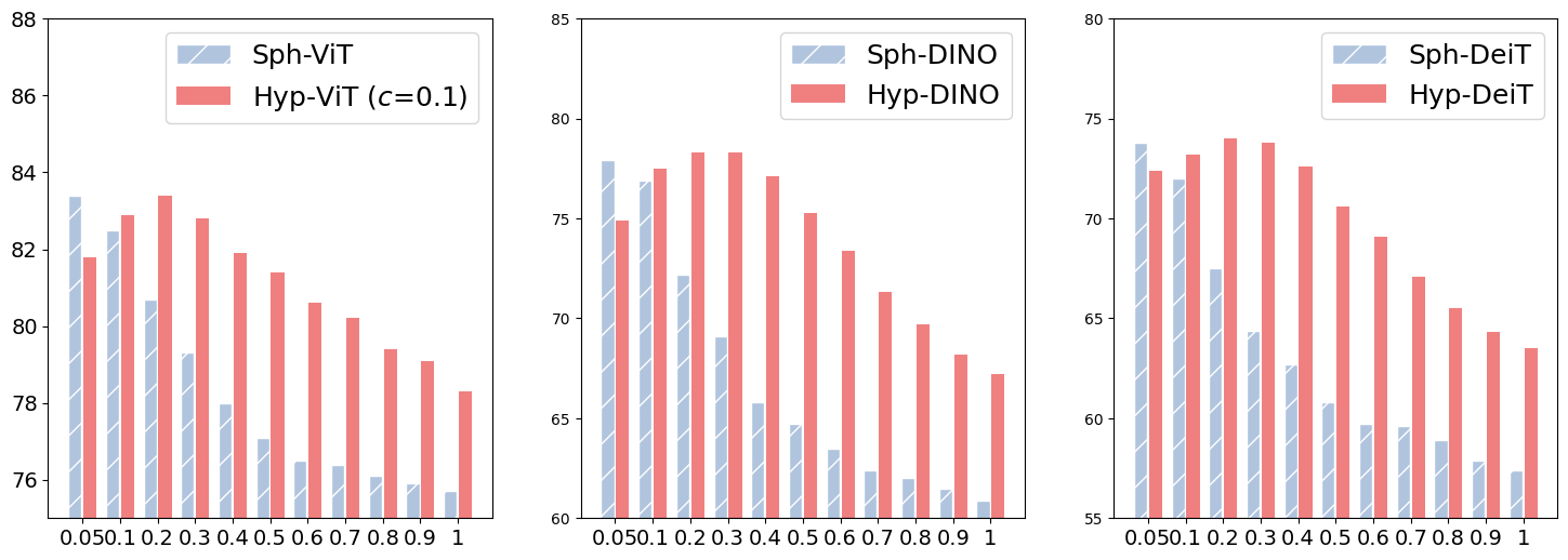
Figure 4: Recall of 1K metric comparison of models trained with different temperatures $\tau$ using CUB-200-2011 dataset. The x-axis indicates different $\tau$. “Sph-” are versions with hypersphere embeddings optimized using $D_{cos}$, “Hyp-” are versions with hyperbolic embeddings optimized using $D_{hyp}$. “ViT”, “DINO”, “DeiT” indicates the pretraining for the vision transformer encoders. For “Hyp-” we fix the curvature parameter $c=0.1$

References

- [1] Relja Arandjelovic and Andrew Zisserman. Objects that sound. In Proceedings of the European conference on computer vision (ECCV), pages 435–451, 2018.
- [2] Sanjeev Arora, Hrishikesh Khandeparkar, Mikhail Khodak, Orestis Plevrakis, and Nikunj Saunshi. A theoretical analysis of contrastive unsupervised representation learning. arXiv preprint arXiv:1902.09229, 2019.
- [3] Mina Ghadimi Atigh, Julian Schoep, Erman Acar, Nanne van Noord, and Pascal Mettes. Hyperbolic image segmentation. In Proceedings of the IEEE/CVF Conference on Computer Vision and Pattern Recognition, pages 4453–4462, 2022.
- [4] Philip Bachman, R Devon Hjelm, and William Buchwalter. Learning representations by maximizing mutual information across views. Advances in neural information processing systems, 32, 2019.
- [5] Avrim Blum and Tom Mitchell. Combining labeled and unlabeled data with co-training. In Proceedings of the eleventh annual conference on Computational learning theory, pages 92–100, 1998.
- [6] Michael M Bronstein, Joan Bruna, Yann LeCun, Arthur Szlam, and Pierre Vandergheynst. Geometric deep learning: going beyond euclidean data. IEEE Signal Processing Magazine, 34(4):18–42, 2017.
- [7] Maxime Bucher, Stéphane Herbin, and Frédéric Jurie. Improving semantic embedding consistency by metric learning for zero-shot classiffication. In Computer Vision–ECCV 2016: 14th European Conference, Amsterdam, The Netherlands, October 11-14, 2016, Proceedings, Part V 14, pages 730–746. Springer, 2016.
- [8] Fatih Cakir, Kun He, Xide Xia, Brian Kulis, and Stan Sclaroff. Deep metric learning to rank. In 2019 IEEE/CVF Conference on Computer Vision and Pattern Recognition (CVPR), pages 1861–1870, 2019.
- [9] James W Cannon, William J Floyd, Richard Kenyon, Walter R Parry, et al. Hyperbolic geometry. Flavors of geometry, 31(59-115):2, 1997.
- [10] Qiong Cao, Yiming Ying, and Peng Li. Similarity metric learning for face recognition. In Proceedings of the IEEE international conference on computer vision, pages 2408–2415, 2013.
- [11] Mathilde Caron, Ishan Misra, Julien Mairal, Priya Goyal, Piotr Bojanowski, and Armand Joulin. Unsupervised learning of visual features by contrasting cluster assignments. Advances in Neural Information Processing Systems, 33:9912–9924, 2020.
- [12] Mathilde Caron, Hugo Touvron, Ishan Misra, Hervé Jégou, Julien Mairal, Piotr Bojanowski, and Armand Joulin. Emerging properties in self-supervised vision transformers. In Proceedings of the IEEE/CVF International Conference on Computer Vision (ICCV), pages 9650–9660, October 2021.
- [13] Binghui Chen and Weihong Deng. Hybrid-attention based decoupled metric learning for zero-shot image retrieval. In Proceedings of the IEEE/CVF conference on computer vision and pattern recognition, pages 2750–2759, 2019.
- [14] Ting Chen, Simon Kornblith, Mohammad Norouzi, and Geoffrey Hinton. A simple framework for contrastive learning of visual representations. In International conference on machine learning, pages 1597–1607. PMLR, 2020.
- [15] Ting Chen, Simon Kornblith, Kevin Swersky, Mohammad Norouzi, and Geoffrey E Hinton. Big self-supervised models are strong semi-supervised learners. Advances in neural information processing systems, 33:22243–22255, 2020.
- [16] Ting Chen, Calvin Luo, and Lala Li. Intriguing properties of contrastive losses. Advances in Neural Information Processing Systems, 34, 2021.
- [17] Weihua Chen, Xiaotang Chen, Jianguo Zhang, and Kaiqi Huang. Beyond triplet loss: a deep quadruplet network for person re-identification. In Proceedings of the IEEE conference on computer vision and pattern recognition, pages 403–412, 2017.
- [18] Xinlei Chen, Haoqi Fan, Ross Girshick, and Kaiming He. Improved baselines with momentum contrastive learning. arXiv preprint arXiv:2003.04297, 2020.
- [19] Sumit Chopra, Raia Hadsell, and Yann LeCun. Learning a similarity metric discriminatively, with application to face verification. In 2005 IEEE Computer Society Conference on Computer Vision and Pattern Recognition (CVPR’05), volume 1, pages 539–546. IEEE, 2005.
- [20] Ching-Yao Chuang, Joshua Robinson, Yen-Chen Lin, Antonio Torralba, and Stefanie Jegelka. Debiased contrastive learning. Advances in neural information processing systems, 33:8765–8775, 2020.
- [21] J. Deng, W. Dong, R. Socher, L.-J. Li, K. Li, and L. Fei-Fei. ImageNet: A Large-Scale Hierarchical Image Database. In CVPR09, 2009.
- [22] Alexey Dosovitskiy, Lucas Beyer, Alexander Kolesnikov, Dirk Weissenborn, Xiaohua Zhai, Thomas Unterthiner, Mostafa Dehghani, Matthias Minderer, Georg Heigold, Sylvain Gelly, et al. An image is worth 16x16 words: Transformers for image recognition at scale. arXiv preprint arXiv:2010.11929, 2020.
- [23] Alexey Dosovitskiy, Lucas Beyer, Alexander Kolesnikov, Dirk Weissenborn, Xiaohua Zhai, Thomas Unterthiner, Mostafa Dehghani, Matthias Minderer, Georg Heigold, Sylvain Gelly, Jakob Uszkoreit, and Neil Houlsby. An image is worth 16x16 words: Transformers for image recognition at scale. ICLR, 2021.
- [24] Alaaeldin El-Nouby, Natalia Neverova, Ivan Laptev, and Hervé Jégou. Training vision transformers for image retrieval. arXiv preprint arXiv:2102.05644, 2021.
- [25] Aleksandr Ermolov, Leyla Mirvakhabova, Valentin Khrulkov, Nicu Sebe, and Ivan Oseledets. Hyperbolic vision transformers: Combining improvements in metric learning. In Proceedings of the IEEE/CVF Conference on Computer Vision and Pattern Recognition, pages 7409–7419, 2022.
- [26] Pengfei Fang, Mehrtash Harandi, and Lars Petersson. Kernel methods in hyperbolic spaces. In Proceedings of the IEEE/CVF International Conference on Computer Vision, pages 10665–10674, 2021.
- [27] Octavian Ganea, Gary Bécigneul, and Thomas Hofmann. Hyperbolic neural networks. Advances in neural information processing systems, 31, 2018.
- [28] Zhi Gao, Yuwei Wu, Yunde Jia, and Mehrtash Harandi. Curvature generation in curved spaces for few-shot learning. In Proceedings of the IEEE/CVF International Conference on Computer Vision, pages 8691–8700, 2021.
- [29] Songwei Ge, Shlok Mishra, Simon Kornblith, Chun-Liang Li, and David Jacobs. Hyperbolic contrastive learning for visual representations beyond objects. arXiv preprint arXiv:2212.00653, 2022.
- [30] Songwei Ge, Shlok Mishra, Chun-Liang Li, Haohan Wang, and David Jacobs. Robust contrastive learning using negative samples with diminished semantics. Advances in Neural Information Processing Systems, 34, 2021.
- [31] Weifeng Ge. Deep metric learning with hierarchical triplet loss. In Proceedings of the European Conference on Computer Vision (ECCV), pages 269–285, 2018.
- [32] Jean-Bastien Grill, Florian Strub, Florent Altché, Corentin Tallec, Pierre Richemond, Elena Buchatskaya, Carl Doersch, Bernardo Avila Pires, Zhaohan Guo, Mohammad Gheshlaghi Azar, et al. Bootstrap your own latent-a new approach to self-supervised learning. Advances in Neural Information Processing Systems, 33:21271–21284, 2020.
- [33] Yunhui Guo, Xudong Wang, Yubei Chen, and Stella X Yu. Clipped hyperbolic classifiers are super-hyperbolic classifiers. In Proceedings of the IEEE/CVF Conference on Computer Vision and Pattern Recognition, pages 11–20, 2022.
- [34] Raia Hadsell, Sumit Chopra, and Yann LeCun. Dimensionality reduction by learning an invariant mapping. In 2006 IEEE Computer Society Conference on Computer Vision and Pattern Recognition (CVPR’06), volume 2, pages 1735–1742. IEEE, 2006.
- [35] Bing He, Jia Li, Yifan Zhao, and Yonghong Tian. Part-regularized near-duplicate vehicle re-identification. In Proceedings of the IEEE/CVF Conference on Computer Vision and Pattern Recognition, pages 3997–4005, 2019.
- [36] Kaiming He, Haoqi Fan, Yuxin Wu, Saining Xie, and Ross Girshick. Momentum contrast for unsupervised visual representation learning. In Proceedings of the IEEE/CVF conference on computer vision and pattern recognition, pages 9729–9738, 2020.
- [37] Kaiming He, Xiangyu Zhang, Shaoqing Ren, and Jian Sun. Deep residual learning for image recognition. In Proceedings of the IEEE Conference on Computer Vision and Pattern Recognition (CVPR), June 2016.
- [38] R Devon Hjelm, Alex Fedorov, Samuel Lavoie-Marchildon, Karan Grewal, Phil Bachman, Adam Trischler, and Yoshua Bengio. Learning deep representations by mutual information estimation and maximization. arXiv preprint arXiv:1808.06670, 2018.
- [39] Steven CH Hoi, Wei Liu, and Shih-Fu Chang. Semi-supervised distance metric learning for collaborative image retrieval and clustering. ACM Transactions on Multimedia Computing, Communications, and Applications (TOMM), 6(3):1–26, 2010.
- [40] Qianjiang Hu, Xiao Wang, Wei Hu, and Guo-Jun Qi. Adco: Adversarial contrast for efficient learning of unsupervised representations from self-trained negative adversaries. In Proceedings of the IEEE/CVF Conference on Computer Vision and Pattern Recognition, pages 1074–1083, 2021.
- [41] Zhiwu Huang, Ruiping Wang, Shiguang Shan, and Xilin Chen. Projection metric learning on grassmann manifold with application to video based face recognition. In Proceedings of the IEEE conference on computer vision and pattern recognition, pages 140–149, 2015.
- [42] Sergey Ioffe and Christian Szegedy. Batch normalization: Accelerating deep network training by reducing internal covariate shift. In International conference on machine learning, pages 448–456. PMLR, 2015.
- [43] Pierre Jacob, David Picard, Aymeric Histace, and Edouard Klein. Metric learning with horde: High-order regularizer for deep embeddings. In Proceedings of the IEEE/CVF International Conference on Computer Vision, pages 6539–6548, 2019.
- [44] Ashish Jaiswal, Ashwin Ramesh Babu, Mohammad Zaki Zadeh, Debapriya Banerjee, and Fillia Makedon. A survey on contrastive self-supervised learning. Technologies, 9(1):2, 2020.
- [45] Huajie Jiang, Ruiping Wang, Shiguang Shan, and Xilin Chen. Adaptive metric learning for zero-shot recognition. IEEE Signal Processing Letters, 26(9):1270–1274, 2019.
- [46] Qing-Yuan Jiang, Yi He, Gen Li, Jian Lin, Lei Li, and Wu-Jun Li. Svd: A large-scale short video dataset for near-duplicate video retrieval. In Proceedings of the IEEE/CVF International Conference on Computer Vision, pages 5281–5289, 2019.
- [47] Wen Jiang, Kai Huang, Jie Geng, and Xinyang Deng. Multi-scale metric learning for few-shot learning. IEEE Transactions on Circuits and Systems for Video Technology, 31(3):1091–1102, 2020.
- [48] Yannis Kalantidis, Mert Bulent Sariyildiz, Noe Pion, Philippe Weinzaepfel, and Diane Larlus. Hard negative mixing for contrastive learning. Advances in Neural Information Processing Systems, 33:21798–21809, 2020.
- [49] Valentin Khrulkov, Leyla Mirvakhabova, Evgeniya Ustinova, Ivan Oseledets, and Victor Lempitsky. Hyperbolic image embeddings. In Proceedings of the IEEE/CVF Conference on Computer Vision and Pattern Recognition, pages 6418–6428, 2020.
- [50] Sungyeon Kim, Dongwon Kim, Minsu Cho, and Suha Kwak. Proxy anchor loss for deep metric learning. In Proceedings of the IEEE/CVF Conference on Computer Vision and Pattern Recognition (CVPR), June 2020.
- [51] Sungnyun Kim, Gihun Lee, Sangmin Bae, and Se-Young Yun. Mixco: Mix-up contrastive learning for visual representation. arXiv preprint arXiv:2010.06300, 2020.
- [52] Wonsik Kim, Bhavya Goyal, Kunal Chawla, Jungmin Lee, and Keunjoo Kwon. Attention-based ensemble for deep metric learning. In Proceedings of the European Conference on Computer Vision (ECCV), pages 736–751, 2018.
- [53] Giorgos Kordopatis-Zilos, Symeon Papadopoulos, Ioannis Patras, and Yiannis Kompatsiaris. Near-duplicate video retrieval with deep metric learning. In Proceedings of the IEEE international conference on computer vision workshops, pages 347–356, 2017.
- [54] Jonathan Krause, Michael Stark, Jia Deng, and Li Fei-Fei. 3d object representations for fine-grained categorization. In 2013 IEEE International Conference on Computer Vision Workshops, pages 554–561, 2013.
- [55] Kibok Lee, Yian Zhu, Kihyuk Sohn, Chun-Liang Li, Jinwoo Shin, and Honglak Lee. i-mix: A domain-agnostic strategy for contrastive representation learning. arXiv preprint arXiv:2010.08887, 2020.
- [56] Chunyuan Li, Xiujun Li, Lei Zhang, Baolin Peng, Mingyuan Zhou, and Jianfeng Gao. Self-supervised pre-training with hard examples improves visual representations. arXiv preprint arXiv:2012.13493, 2020.
- [57] Junnan Li, Pan Zhou, Caiming Xiong, and Steven CH Hoi. Prototypical contrastive learning of unsupervised representations. arXiv preprint arXiv:2005.04966, 2020.
- [58] Zechao Li and Jinhui Tang. Weakly supervised deep metric learning for community-contributed image retrieval. IEEE Transactions on Multimedia, 17(11):1989–1999, 2015.
- [59] Zhaowen Li, Yousong Zhu, Fan Yang, Wei Li, Chaoyang Zhao, Yingying Chen, Zhiyang Chen, Jiahao Xie, Liwei Wu, Rui Zhao, et al. Univip: A unified framework for self-supervised visual pre-training. arXiv preprint arXiv:2203.06965, 2022.
- [60] Shengcai Liao and Stan Z Li. Efficient psd constrained asymmetric metric learning for person re-identification. In Proceedings of the IEEE international conference on computer vision, pages 3685–3693, 2015.
- [61] Fangfei Lin, Bing Bai, Kun Bai, Yazhou Ren, Peng Zhao, and Zenglin Xu. Contrastive multi-view hyperbolic hierarchical clustering. arXiv preprint arXiv:2205.02618, 2022.
- [62] Jiahong Liu, Menglin Yang, Min Zhou, Shanshan Feng, and Philippe Fournier-Viger. Enhancing hyperbolic graph embeddings via contrastive learning. arXiv preprint arXiv:2201.08554, 2022.
- [63] Shaoteng Liu, Jingjing Chen, Liangming Pan, Chong-Wah Ngo, Tat-Seng Chua, and Yu-Gang Jiang. Hyperbolic visual embedding learning for zero-shot recognition. In Proceedings of the IEEE/CVF conference on computer vision and pattern recognition, pages 9273–9281, 2020.
- [64] Weiyang Liu, Yandong Wen, Zhiding Yu, Ming Li, Bhiksha Raj, and Le Song. Sphereface: Deep hypersphere embedding for face recognition. In Proceedings of the IEEE conference on computer vision and pattern recognition, pages 212–220, 2017.
- [65] Lajanugen Logeswaran and Honglak Lee. An efficient framework for learning sentence representations. arXiv preprint arXiv:1803.02893, 2018.
- [66] Ilya Loshchilov and Frank Hutter. Decoupled weight decay regularization. In International Conference on Learning Representations, 2019.
- [67] Shlok Mishra, Anshul Shah, Ankan Bansal, Abhyuday Jagannatha, Abhishek Sharma, David Jacobs, and Dilip Krishnan. Object-aware cropping for self-supervised learning. arXiv preprint arXiv:2112.00319, 2021.
- [68] Ishan Misra and Laurens van der Maaten. Self-supervised learning of pretext-invariant representations. In Proceedings of the IEEE/CVF Conference on Computer Vision and Pattern Recognition, pages 6707–6717, 2020.
- [69] Antonio Montanaro, Diego Valsesia, and Enrico Magli. Rethinking the compositionality of point clouds through regularization in the hyperbolic space. arXiv preprint arXiv:2209.10318, 2022.
- [70] Yair Movshovitz-Attias, Alexander Toshev, Thomas K Leung, Sergey Ioffe, and Saurabh Singh. No fuss distance metric learning using proxies. In Proceedings of the IEEE International Conference on Computer Vision, pages 360–368, 2017.
- [71] Kevin Musgrave, Serge Belongie, and Ser-Nam Lim. A metric learning reality check. In European Conference on Computer Vision, pages 681–699. Springer, 2020.
- [72] Maximillian Nickel and Douwe Kiela. Poincaré embeddings for learning hierarchical representations. Advances in neural information processing systems, 30, 2017.
- [73] Maximillian Nickel and Douwe Kiela. Learning continuous hierarchies in the lorentz model of hyperbolic geometry. In International Conference on Machine Learning, pages 3779–3788. PMLR, 2018.
- [74] Hyun Oh Song, Yu Xiang, Stefanie Jegelka, and Silvio Savarese. Deep metric learning via lifted structured feature embedding. In Proceedings of the IEEE conference on computer vision and pattern recognition, pages 4004–4012, 2016.
- [75] Aaron van den Oord, Yazhe Li, and Oriol Vinyals. Representation learning with contrastive predictive coding. arXiv preprint arXiv:1807.03748, 2018.
- [76] Michael Opitz, Georg Waltner, Horst Possegger, and Horst Bischof. Deep metric learning with bier: Boosting independent embeddings robustly. IEEE transactions on pattern analysis and machine intelligence, 42(2):276–290, 2018.
- [77] Adam Paszke, Sam Gross, Francisco Massa, Adam Lerer, James Bradbury, Gregory Chanan, Trevor Killeen, Zeming Lin, Natalia Gimelshein, Luca Antiga, et al. Pytorch: An imperative style, high-performance deep learning library. Advances in neural information processing systems, 32, 2019.
- [78] Wei Peng, Tuomas Varanka, Abdelrahman Mostafa, Henglin Shi, and Guoying Zhao. Hyperbolic deep neural networks: A survey. IEEE Transactions on Pattern Analysis and Machine Intelligence, 44(12):10023–10044, 2021.
- [79] Xiangyu Peng, Kai Wang, Zheng Zhu, and Yang You. Crafting better contrastive views for siamese representation learning. arXiv preprint arXiv:2202.03278, 2022.
- [80] Senthil Purushwalkam and Abhinav Gupta. Demystifying contrastive self-supervised learning: Invariances, augmentations and dataset biases. Advances in Neural Information Processing Systems, 33:3407–3418, 2020.
- [81] Qi Qian, Lei Shang, Baigui Sun, Juhua Hu, Hao Li, and Rong Jin. Softtriple loss: Deep metric learning without triplet sampling. In Proceedings of the IEEE/CVF International Conference on Computer Vision, pages 6450–6458, 2019.
- [82] Limeng Qiao, Yemin Shi, Jia Li, Yaowei Wang, Tiejun Huang, and Yonghong Tian. Transductive episodic-wise adaptive metric for few-shot learning. In Proceedings of the IEEE/CVF International Conference on Computer Vision, pages 3603–3612, 2019.
- [83] Sucheng Ren, Huiyu Wang, Zhengqi Gao, Shengfeng He, Alan Yuille, Yuyin Zhou, and Cihang Xie. A simple data mixing prior for improving self-supervised learning. In CVPR, 2022.
- [84] Joshua Robinson, Ching-Yao Chuang, Suvrit Sra, and Stefanie Jegelka. Contrastive learning with hard negative samples. arXiv preprint arXiv:2010.04592, 2020.
- [85] Joshua David Robinson, Ching-Yao Chuang, Suvrit Sra, and Stefanie Jegelka. Contrastive learning with hard negative samples. In International Conference on Learning Representations, 2021.
- [86] Karsten Roth, Biagio Brattoli, and Bjorn Ommer. Mic: Mining interclass characteristics for improved metric learning. In Proceedings of the IEEE/CVF International Conference on Computer Vision, pages 8000–8009, 2019.
- [87] Olga Russakovsky, Jia Deng, Hao Su, Jonathan Krause, Sanjeev Satheesh, Sean Ma, Zhiheng Huang, Andrej Karpathy, Aditya Khosla, Michael Bernstein, Alexander C. Berg, and Li Fei-Fei. Imagenet large scale visual recognition challenge. International Journal of Computer Vision (IJCV), 115(3):211–252, 2015.
- [88] Rik Sarkar. Low distortion delaunay embedding of trees in hyperbolic plane. In International symposium on graph drawing, pages 355–366. Springer, 2012.
- [89] Andrew M. Saxe, James L. McClelland, and Surya Ganguli. Exact solutions to the nonlinear dynamics of learning in deep linear neural networks. In Yoshua Bengio and Yann LeCun, editors, 2nd International Conference on Learning Representations, ICLR 2014, Banff, AB, Canada, April 14-16, 2014, Conference Track Proceedings, 2014.
- [90] Florian Schroff, Dmitry Kalenichenko, and James Philbin. Facenet: A unified embedding for face recognition and clustering. 2015 IEEE Conference on Computer Vision and Pattern Recognition (CVPR), Jun 2015.
- [91] Ramprasaath R Selvaraju, Karan Desai, Justin Johnson, and Nikhil Naik. Casting your model: Learning to localize improves self-supervised representations. In Proceedings of the IEEE/CVF Conference on Computer Vision and Pattern Recognition, pages 11058–11067, 2021.
- [92] Pierre Sermanet, Corey Lynch, Yevgen Chebotar, Jasmine Hsu, Eric Jang, Stefan Schaal, Sergey Levine, and Google Brain. Time-contrastive networks: Self-supervised learning from video. In 2018 IEEE international conference on robotics and automation (ICRA), pages 1134–1141. IEEE, 2018.
- [93] Anshul Shah, Suvrit Sra, Rama Chellappa, and Anoop Cherian. Max-margin contrastive learning. In Proceedings of the AAAI Conference on Artificial Intelligence, volume 36, pages 8220–8230, 2022.
- [94] Zhiqiang Shen, Zechun Liu, Zhuang Liu, Marios Savvides, Trevor Darrell, and Eric Xing. Un-mix: Rethinking image mixtures for unsupervised visual representation learning. arXiv preprint arXiv:2003.05438, 2020.
- [95] Abhishek Sinha, Kumar Ayush, Jiaming Song, Burak Uzkent, Hongxia Jin, and Stefano Ermon. Negative data augmentation. In International Conference on Learning Representations, 2021.
- [96] Jake Snell, Kevin Swersky, and Richard Zemel. Prototypical networks for few-shot learning. Advances in neural information processing systems, 30, 2017.
- [97] Kihyuk Sohn. Improved deep metric learning with multi-class n-pair loss objective. In D. Lee, M. Sugiyama, U. Luxburg, I. Guyon, and R. Garnett, editors, Advances in Neural Information Processing Systems, volume 29. Curran Associates, Inc., 2016.
- [98] Kihyuk Sohn. Improved deep metric learning with multi-class n-pair loss objective. Advances in neural information processing systems, 29, 2016.
- [99] Hyun Oh Song, Yu Xiang, Stefanie Jegelka, and Silvio Savarese. Deep metric learning via lifted structured feature embedding. In IEEE Conference on Computer Vision and Pattern Recognition (CVPR), 2016.
- [100] Aravind Srinivas, Michael Laskin, and Pieter Abbeel. Curl: Contrastive unsupervised representations for reinforcement learning. arXiv preprint arXiv:2004.04136, 2020.
- [101] Andreas Steiner, Alexander Kolesnikov, Xiaohua Zhai, Ross Wightman, Jakob Uszkoreit, and Lucas Beyer. How to train your vit? data, augmentation, and regularization in vision transformers. arXiv preprint arXiv:2106.10270, 2021.
- [102] Yumin Suh, Bohyung Han, Wonsik Kim, and Kyoung Mu Lee. Stochastic class-based hard example mining for deep metric learning. In 2019 IEEE/CVF Conference on Computer Vision and Pattern Recognition (CVPR), pages 7244–7252, 2019.
- [103] Flood Sung, Yongxin Yang, Li Zhang, Tao Xiang, Philip HS Torr, and Timothy M Hospedales. Learning to compare: Relation network for few-shot learning. In Proceedings of the IEEE conference on computer vision and pattern recognition, pages 1199–1208, 2018.
- [104] Christian Szegedy, Wei Liu, Yangqing Jia, Pierre Sermanet, Scott Reed, Dragomir Anguelov, Dumitru Erhan, Vincent Vanhoucke, and Andrew Rabinovich. Going deeper with convolutions. In Proceedings of the IEEE conference on computer vision and pattern recognition, pages 1–9, 2015.
- [105] Eu Wern Teh, Terrance DeVries, and Graham W Taylor. Proxynca++: Revisiting and revitalizing proxy neighborhood component analysis. In European Conference on Computer Vision, pages 448–464. Springer, 2020.
- [106] Yonglong Tian, Dilip Krishnan, and Phillip Isola. Contrastive multiview coding. arXiv preprint arXiv:1906.05849, 2019.
- [107] Yonglong Tian, Dilip Krishnan, and Phillip Isola. Contrastive multiview coding. In European conference on computer vision, pages 776–794. Springer, 2020.
- [108] Yonglong Tian, Chen Sun, Ben Poole, Dilip Krishnan, Cordelia Schmid, and Phillip Isola. What makes for good views for contrastive learning? Advances in Neural Information Processing Systems, 33:6827–6839, 2020.
- [109] Hugo Touvron, Matthieu Cord, Matthijs Douze, Francisco Massa, Alexandre Sablayrolles, and Hervé Jégou. Training data-efficient image transformers & distillation through attention. In International Conference on Machine Learning, pages 10347–10357. PMLR, 2021.
- [110] Michael Tschannen, Josip Djolonga, Marvin Ritter, Aravindh Mahendran, Neil Houlsby, Sylvain Gelly, and Mario Lucic. Self-supervised learning of video-induced visual invariances. In Proceedings of the IEEE/CVF Conference on Computer Vision and Pattern Recognition, pages 13806–13815, 2020.
- [111] Abraham Albert Ungar. Analytic hyperbolic geometry and Albert Einstein’s special theory of relativity. World Scientific, 2008.
- [112] Abraham Albert Ungar. A gyrovector space approach to hyperbolic geometry. Synthesis Lectures on Mathematics and Statistics, 1(1):1–194, 2008.
- [113] Vikas Verma, Thang Luong, Kenji Kawaguchi, Hieu Pham, and Quoc Le. Towards domain-agnostic contrastive learning. In International Conference on Machine Learning, pages 10530–10541. PMLR, 2021.
- [114] Feng Wang and Huaping Liu. Understanding the behaviour of contrastive loss. In Proceedings of the IEEE/CVF conference on computer vision and pattern recognition, pages 2495–2504, 2021.
- [115] Jian Wang, Feng Zhou, Shilei Wen, Xiao Liu, and Yuanqing Lin. Deep metric learning with angular loss. In Proceedings of the IEEE international conference on computer vision, pages 2593–2601, 2017.
- [116] Tongzhou Wang and Phillip Isola. Understanding contrastive representation learning through alignment and uniformity on the hypersphere. In International Conference on Machine Learning, pages 9929–9939. PMLR, 2020.
- [117] Xun Wang, Xintong Han, Weilin Huang, Dengke Dong, and Matthew R Scott. Multi-similarity loss with general pair weighting for deep metric learning. In Proceedings of the IEEE/CVF Conference on Computer Vision and Pattern Recognition, pages 5022–5030, 2019.
- [118] Xun Wang, Haozhi Zhang, Weilin Huang, and Matthew R Scott. Cross-batch memory for embedding learning. In Proceedings of the IEEE/CVF Conference on Computer Vision and Pattern Recognition, pages 6388–6397, 2020.
- [119] Kilian Q Weinberger and Lawrence K Saul. Distance metric learning for large margin nearest neighbor classification. Journal of machine learning research, 10(2), 2009.
- [120] P. Welinder, S. Branson, T. Mita, C. Wah, F. Schroff, S. Belongie, and P. Perona. Caltech-UCSD Birds 200. Technical Report CNS-TR-2010-001, California Institute of Technology, 2010.
- [121] Zhenzhen Weng, Mehmet Giray Ogut, Shai Limonchik, and Serena Yeung. Unsupervised discovery of the long-tail in instance segmentation using hierarchical self-supervision. In Proceedings of the IEEE/CVF Conference on Computer Vision and Pattern Recognition, pages 2603–2612, 2021.
- [122] Chao-Yuan Wu, R Manmatha, Alexander J Smola, and Philipp Krahenbuhl. Sampling matters in deep embedding learning. In Proceedings of the IEEE international conference on computer vision, pages 2840–2848, 2017.
- [123] Chao-Yuan Wu, R Manmatha, Alexander J Smola, and Philipp Krahenbuhl. Sampling matters in deep embedding learning. In Proceedings of the IEEE International Conference on Computer Vision, pages 2840–2848, 2017.
- [124] Zhirong Wu, Yuanjun Xiong, Stella X Yu, and Dahua Lin. Unsupervised feature learning via non-parametric instance discrimination. In Proceedings of the IEEE conference on computer vision and pattern recognition, pages 3733–3742, 2018.
- [125] Tong Xiao, Shuang Li, Bochao Wang, Liang Lin, and Xiaogang Wang. Joint detection and identification feature learning for person search. In Proceedings of the IEEE conference on computer vision and pattern recognition, pages 3415–3424, 2017.
- [126] Chang Xu, Dacheng Tao, and Chao Xu. A survey on multi-view learning. arXiv preprint arXiv:1304.5634, 2013.
- [127] Dong Yi, Zhen Lei, Shengcai Liao, and Stan Z Li. Deep metric learning for person re-identification. In 2014 22nd international conference on pattern recognition, pages 34–39. IEEE, 2014.
- [128] Yun Yue, Fangzhou Lin, Kazunori D Yamada, and Ziming Zhang. Hyperbolic contrastive learning. arXiv preprint arXiv:2302.01409, 2023.
- [129] Andrew Zhai and Hao-Yu Wu. Classification is a strong baseline for deep metric learning. arXiv preprint arXiv:1811.12649, 2018.
- [130] Hongyi Zhang, Moustapha Cisse, Yann N Dauphin, and David Lopez-Paz. mixup: Beyond empirical risk minimization. arXiv preprint arXiv:1710.09412, 2017.
- [131] Stephan Zheng, Yang Song, Thomas Leung, and Ian Goodfellow. Improving the robustness of deep neural networks via stability training. In Proceedings of the ieee conference on computer vision and pattern recognition, pages 4480–4488, 2016.