Deep Hankel matrices with random elements

Abstract

Willems’ fundamental lemma enables a trajectory-based characterization of linear systems through data-based Hankel matrices. However, in the presence of measurement noise, we ask: Is this noisy Hankel-based model expressive enough to re-identify itself? In other words, we study the output prediction accuracy from recursively applying the same persistently exciting input sequence to the model. We find an asymptotic connection to this self-consistency question in terms of the amount of data. More importantly, we also connect this question to the depth (number of rows) of the Hankel model, showing the simple act of reconfiguring a finite dataset significantly improves accuracy. We apply these insights to find a parsimonious depth for LQR problems over the trajectory space.

1 Introduction

This paper concerns Hankel matrices of the form

$$H_{L}(z)=\begin{bmatrix}z_{0}&z_{1}&\ldots&z_{N-L}\\ z_{1}&z_{2}&\ldots&z_{N-L+1}\\ \vdots&\vdots&\ddots&\vdots\\ z_{L-1}&z_{L}&\ldots&z_{N-1}\end{bmatrix},$$ (2)

where each $z_{i}\sim\mathcal{N}(0,1)$. This structure arises naturally in the context of a nominal LTI system whose state $x$ evolves in $\mathbb{R}^{n}$:

$$x_{t+1} =Ax_{t}+Bu_{t}$$ (3)

$$\widehat{y}_{t} =Cx_{t} t=0,1,2,\ldots$$

By organizing the inputs and outputs of the system in Hankel matrices $H_{L}(u)$ and $H_{L}(\widehat{y})$, respectively, Willems’ fundamental lemma characterizes the trajectory space of Eq. 3 through the matrix-vector product $\begin{bmatrix}H_{L}(u)\\ H_{L}(\widehat{y})\end{bmatrix}\alpha$. (A precise formulation is given in Section 2.) Taking the input to be a Gaussian probing signal $u$ and the output to be subject to measurement noise, $y=\widehat{y}+\omega$, we arrive at the following situation:

$$\begin{bmatrix}H_{L}(u)\\ H_{L}(y)\end{bmatrix}\alpha=\underbrace{\begin{bmatrix}H_{L}(u)\\ H_{L}(\widehat{y})\end{bmatrix}\alpha}_{\text{True trajectory}}+\underbrace{\begin{bmatrix}0\\ H_{L}(\omega)\end{bmatrix}\alpha}_{\text{Error}}$$ (4)

The question then arises: which term dominates the right-hand side? To give the problem a little more structure, we assume the input and output noise profiles are fixed, and we are only able to manipulate the depth and width, which are characterized by the window length $L$ and the number of samples $N$, respectively. Therefore, we are interested in the interplay between the amount of data, the depth of the Hankel matrices, and the overall error.

In practice, we employ a self-consistency test to determine a sufficiently expressive $L$ from a fixed dataset. That is, we use the same input sequence $u$ in Eq. 4 to iteratively predict some output sequence $\tilde{y}$ with the hope that it is close to the underlying sequence $\widehat{y}$. We show in Eq. 7 and Section 3.2 that increasing the depth mitigates the effect of the noise term in Eq. 4. This is illustrated in Fig. 1 as motivation and explained in more detail in Section 5.

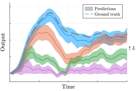
Figure 1: For a fixed-size dataset, adjusting the depth of the input-output Hankel matrices dramatically improves self-consistency. Results are for $L=2,5,10,20$ and each color corresponds to $50$ rollouts with different output noise instances but a fixed input sequence.

The most similar works to ours are Coulson et al. (2023); Guo et al. (2023); Yan et al. (2023). However, none of them consider the matrix depth in their formulation. Coulson et al. (2023) propose casting Willems’ lemma in terms of a minimum singular value criterion, rather than the standard binary rank condition. Guo et al. (2023) consider perturbations to the data-based model, similar to Eq. 4, but their analysis is based on Page matrices and the assumption that the perturbation has a known upper bound. (We use Hankel matrices and show the random perturbation in Eq. 4 is unbounded.) Yan et al. (2023) examine the approximation properties of noisy Hankel models, but their analysis is framed in terms of independent rollouts rather than trajectory length and depth. More related work is discussed in Section 4. Finally, the authors’ work Lawrence et al. (2024) contains similar analytical tools used here, but the setting is completely different: this work zooms in on the approximation properties of random Hankel matrices, while Lawrence et al. (2024) uses the behavioral setting for reinforcement learning problems.

2 Background

Notation.  We often write a vector of sequential variables as $\overline{z}=\left[z_{0},\ldots,z_{k}\right]^{\top}$ when the number of elements is clear from context. When specifying the time indices, we write $\overline{z}_{0:k}$. The spectral radius function $\rho$ ingests a square matrix and returns a nonnegative scalar: $\rho(M)=\max\left\{\left|\lambda\right|\,:\,\lambda\in\mathbb{C},\ Mv=\lambda v\ \text{for some}\ v\neq 0\right\}.$ We use $\lVert\cdot\rVert$ for the Euclidean norm and $\lVert\cdot\rVert_{F}$ for the Frobenius norm. $A^{+}$ denotes the Moore-Penrose inverse, or pseudoinverse, of the matrix $A$.

Willems’ fundamental lemma. We assume single-input single-output dynamics; however, the following formulation holds for general LTI systems and multidimensional noise. Given an $N$-element sequence $\{z_{t}\}_{t=0}^{N-1}\subset\mathbb{R}$ and an integer $L$, $1\leq L\leq N$, the Hankel matrix of depth $L$ is the $L\times(N-L+1)$ array with the constant skew-diagonal structure $H_{L}(z)$ defined in Eq. 2.

Definition 2.1.

The signal $\{z_{t}\}_{t=0}^{N-1}\subset\mathbb{R}$ is persistently exciting of order $L$ if $\operatorname{rank}(H_{L}(z))=L$.

Definition 2.2.

An input-output sequence $\{u_{t},y_{t}\}_{t=0}^{N-1}$ is a trajectory of LTI system $(A,B,C)$ as in Eq. 3 if there exists a state sequence $\{x_{t}\}_{t=0}^{N-1}$ such that Eq. 3 holds.

We assume the matrices $A,B,C$ in Eq. 3 are unknown, $(A,B)$ is controllable, and $(A,C)$ is observable. This lays the foundation for the following data-driven characterization of LTI systems.

Theorem 2.3 (Willems’ fundamental lemma (van Waarde et al., 2020; Willems et al., 2005)).

Let $\{u_{t},y_{t}\}_{t=0}^{N-1}$ be a trajectory of LTI system $(A,B,C)$ where $u$ is persistently exciting of order $L+n$. Then $\{\overline{u}_{t},\overline{y}_{t}\}_{t=0}^{L-1}$ is a trajectory of $(A,B,C)$ if and only if there exists $\alpha\in\mathbb{R}^{N-L+1}$ such that

$$\begin{bmatrix}H_{L}(u)\\ H_{L}(y)\end{bmatrix}\alpha=\begin{bmatrix}\overline{u}\\ \overline{y}\end{bmatrix}.$$ (5)

Equivalently, one may check if the stacked matrix in Eq. 5 has rank $L+n$ (Coulson et al., 2023). Equation 5 says that a Hankel matrix constructed from sufficiently exciting input-output data contains enough information to serve as a dynamic model.

The standard form above provides a certificate for a given trajectory; from that trajectory, one may also wish to advance it forward in time. To that end, we use Eq. 5 to generate arbitrarily long rollouts from some input sequence $\{\widehat{u}_{t}\}_{t}$ as follows: Given $N$ and vectors $z_{0},\ldots,z_{N}$, let $z=\{z_{t}\}_{t=0}^{N-1}$ and $z^{\prime}=\{z_{t}\}_{t=1}^{N}$. Then define the time-shifted Hankel matrix as follows:

$$H^{\prime}_{L}(z)=H_{L}(z^{\prime}).$$ (6)

If $\alpha$ satisfies Eq. 5, then, assuming $L\geq n$, multiplying $H^{\prime}(y)$ by $\alpha$ is equivalent to advancing the internal state forward, yielding the unique next output trajectory

$${\overline{y}^{\prime}=H^{\prime}(y)\alpha}.$$

Section 2 repeats this procedure for any number of time steps.

[tbp] Data-driven rollout KwInputInput Data $\{u_{k},y_{k}\}_{k=0}^{N}$ with persistently exciting input of order $L+1+n$; Initial trajectory $\{\overline{u}_{k},\overline{y}_{k}\}_{k=0}^{L-1}$; An input sequence $\{\widehat{u}_{t}\}$ for simulation. each $\widehat{u}\in\{\widehat{u}_{t}\}$ Solve for $\alpha$: $\begin{bmatrix}H_{L}(u)\\ H_{L}(y)\end{bmatrix}\alpha=\begin{bmatrix}\overline{u}\\ \overline{y}\end{bmatrix}$  Compute the next element $\overline{y}^{\prime}=H^{\prime}_{L}(y)\alpha$  Queue the next control input $\overline{u}_{L}=\widehat{u}$  Update trajectory: $\{\overline{u}_{k},\overline{y}_{k}\}_{k=0}^{L-1}\leftarrow\{\overline{u}_{k},\overline{y}_{k}\}_{k=1}^{L}$

Tools for analysis.  Our problem setup postulates that the input sequence and output noise are (sub-)Gaussian. To understand the approximation properties of noisy models such as Eq. 4, we analyze the singular values of the purely noisy arrays introduced in Eq. 2. Doing so is related to studying the norm of the pseudoinverse. By extension, we can apply the techniques and results to the full noisy model in Eq. 4. In pursuit of this, we leverage two ingredients: $1$. A Gershgorin disk theorem for generalized eigenvalue problems of the form $Av=\lambda Bv$ (Nakatsukasa, 2011). This gives bounds on the singular values of Hankel matrices using row-wise information. $2$.  The Hanson-Wright inequality (Rudelson and Vershynin, 2013) for analyzing the concentrations of key terms that appear in item $1$.

3 Main results

We first analyze the singular values of random matrices of the form in Eq. 2. This will then give insight into its approximation properties of the full noisy model as a function of $N$ and $L$.

3.1 Singular values of random Hankel matrices

The following theorem establishes that the singular values of $H_{L}=H_{L}(z)$ diverge to infinity with high probability as the amount of data increases.

Theorem 3.1.

For any $L\in\mathbb{N}$, in the context detailed above, there is a sequence $\epsilon_{N}\to 0^{+}$ such that

$$\lim_{N\to\infty}\mathbb{P}\left(\frac{1}{\sigma_{\min}(H_{L})}\leq\epsilon_{N}\right)=1.$$ (7)

See the appendix for a full proof. The main idea is to employ a Gershgorin-type argument to contain all $L$ singular values of $\left(H_{L}H_{L}^{\top}\right)^{-1}$ within shrinking disks around the origin. However, to make the problem tractable, we rewrite it as a generalized eigenvalue problem:

$$Iv=\frac{1}{\sigma^{2}}H_{L}H_{L}^{\top}v$$ (8)

Therefore, we can employ concentration inequalities to analyze the diagonal and off-diagonal terms of $H_{L}H_{L}^{\top}$ in a similar fashion to the classical Gershgorin disk theorem.

The proof of Eq. 7 provides many suitable sequences $\epsilon_{N}\to 0^{+}$. In particular, we arrive at the general estimate:

$$\frac{1}{\sigma^{2}}\leq\frac{1}{(N-L+1)(1-\beta)}\left(1+\frac{\gamma}{1-\gamma}\right),$$ (9)

where ${\beta,\gamma\in(0,1)}$. We therefore want $\beta,\gamma$ to be close to $0$. For example, with a “large” ($N\gg L$) but finite dataset, setting $\beta=\gamma=\frac{1}{L+1}$ leads to the approximation

$$\frac{1}{\sigma}\lessapprox\frac{1}{\mathchoice{{\hbox{$\displaystyle\sqrt{N\,}$}\lower 0.4pt\hbox{\vrule height=6.83331pt,depth=-5.46667pt}}}{{\hbox{$\textstyle\sqrt{N\,}$}\lower 0.4pt\hbox{\vrule height=6.83331pt,depth=-5.46667pt}}}{{\hbox{$\scriptstyle\sqrt{N\,}$}\lower 0.4pt\hbox{\vrule height=4.78333pt,depth=-3.82668pt}}}{{\hbox{$\scriptscriptstyle\sqrt{N\,}$}\lower 0.4pt\hbox{\vrule height=3.41666pt,depth=-2.73334pt}}}}\frac{L+1}{L}.$$ (10)

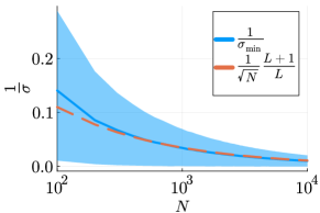
Figure 2: Illustration of Eq. 10.

Therefore, with a fixed amount of data, the bound on the singular values can be reduced by increasing $L$. Of course, increasing $L$ is helpful only up to a point, as the quantity $\frac{L+1}{L}$ decreases to $1$ “slowly” meaning more data are preferable, if available. Moreover, we caution that $L$ cannot be increased arbitrarily, as doing so decreases the underlying probabilities needed for Eq. 7 to hold. Equation 10 is illustrated in Fig. 2 for a fixed $L$. The solid curve is the median inside the interquartile range across $50$ random instances of $H_{L}$.

3.2 A tale of two Gaussians

We can apply the techniques described in Section 3.1 to characterize the singular values of the full noisy model in Eq. 4. In particular, we have two random matrices $H_{L}(u),H_{L}(\omega)$ and a third output component $H_{L}(\widehat{y})$. The input term $H_{L}(u)$ fits the formulation of the previous section and requires no modification. We can leverage this fact to characterize the singular values of the full model. Define $H_{L}$ to be the noisy stacked Hankel matrix in Eq. 4 and $\widehat{H}_{L}$ to be the clean counterpart.

Putting these pieces together in a Gram matrix yields:

$$\begin{multlined}H_{L}H_{L}^{\top}=\widehat{H}_{L}\widehat{H}_{L}^{\top}\\ +\begin{bmatrix}0&0\\ 0&H_{L}(\omega)H_{L}(\omega)^{\top}\end{bmatrix}+\begin{bmatrix}0&H_{L}(u)H_{L}(\omega)^{\top}\\ H_{L}(\omega)H_{L}(u)^{\top}&0\end{bmatrix}+\begin{bmatrix}0&0\\ 0&H_{L}(\widehat{y})H_{L}(\omega)^{\top}+H_{L}(\omega)H_{L}(\widehat{y})^{\top}\end{bmatrix}\end{multlined}H_{L}H_{L}^{\top}=\widehat{H}_{L}\widehat{H}_{L}^{\top}\\ +\begin{bmatrix}0&0\\ 0&H_{L}(\omega)H_{L}(\omega)^{\top}\end{bmatrix}+\begin{bmatrix}0&H_{L}(u)H_{L}(\omega)^{\top}\\ H_{L}(\omega)H_{L}(u)^{\top}&0\end{bmatrix}+\begin{bmatrix}0&0\\ 0&H_{L}(\widehat{y})H_{L}(\omega)^{\top}+H_{L}(\omega)H_{L}(\widehat{y})^{\top}\end{bmatrix}$$ (11)

To align with Willems’ lemma, we are interested in the top $L+n$ eigenvalues of $H_{L}H_{L}^{\top}$. Using standard estimates, we can lower bound $\lambda_{L+n}(H_{L}H_{L}^{\top})$ by $\lambda_{L+n}(\widehat{H}_{L}\widehat{H}_{L}^{\top})+\sum_{i=1}^{3}\lambda_{\min}(M_{i})$ for each remaining matrix $M_{i}$ in Eq. 11. The first term, $\lambda_{L+n}(\widehat{H}_{L}\widehat{H}_{L}^{\top})$, comfortably tends to infinity using the Cauchy interlacing theorem (Coulson et al., 2023; Horn and Johnson, 2012) and Eq. 7. We can disregard the second term in Eq. 11. Finally, the last two terms threaten to shift the momentum away from $+\infty$. The second-to-last term is concentrated around zero due to the classical Gershgorin disk theorem: one can obtain a well-behaved bound similar to Eq. 23 in the proof of Eq. 7. The last term is similar if we assume a positive $c$ such that $\lVert\widehat{y}_{t}\rVert\leq c$ for all $t\geq 0$. (Otherwise, one expects to run into numerical stability issues when computing these singular values for large $N$ and a preconditioner should be used.) Consequently, $\lambda_{L+n}\left(H_{L}H_{L}^{\top}\right)\to\infty$ with high probability as in the case shown in Section 3.1.

3.3 Increasing depth improves self-consistency

In light of the question surrounding Eq. 4, Eq. 7 says the additive error term is not a “small” perturbation to the true data matrix. However, this result still works in our favor. Indeed, writing out the noisy linear system implied by Willems’ fundamental lemma (Eq. 5), $H_{L}\alpha=\begin{bmatrix}\overline{u}\\ \overline{y}\end{bmatrix}$, the minimum-norm solution is $\alpha=H_{L}^{+}\begin{bmatrix}\overline{u}\\ \overline{y}\end{bmatrix}$. Consequently, our results and discussion from Sections 3.1 and 3.2 show that

$$\lim_{N\to\infty}\mathbb{P}\Big{(}\underbrace{\lVert H_{L}^{+}\rVert}_{\frac{1}{\sigma_{L+n}(H_{L})}}\leq\underbrace{\epsilon_{N}}_{\to 0^{+}}\Big{)}=1.$$ (12)

Further, following Eq. 10, increasing $L$ accelerates the convergence by a linear factor.

To see the effect on the prediction accuracy, consider the following evaluation procedure: Run Section 2 where the simulation sequence $\{\widehat{u}_{t}\}=\{u_{k}\}_{k=0}^{N}$. Then, evaluate the RMSE between the resulting outputs $\{\tilde{y}_{t}\}$ and the true measured sequence $\{y_{k}\}_{k=0}^{N}$. Note each prediction has the general form $\tilde{y}_{i}=\left[y_{L}\ldots y_{N}\right]\alpha$ where $\left[y_{L}\ldots y_{N}\right]$ is the last row of $H^{\prime}_{L}(y)$ and $y_{i+L}$ is the target. Then, we see

$$\lVert\tilde{y}_{i}-y_{i+L}\rVert =\lVert\left(\left[\widehat{y}_{L}\ldots\widehat{y}_{N}\right]+\left[\omega_{L}\ldots\omega_{N}\right]\right)\alpha-y_{i+L}\rVert$$ (13)

$$\leq\lVert\left[\widehat{y}_{L}\ldots\widehat{y}_{N}\right]\alpha-y_{i+L}\rVert+\lVert\left[\omega_{L}\ldots\omega_{N}\right]\alpha\rVert$$ (14)

We find that increasing $L$ has two desirable effects: $1$. It improves the bound on $\frac{1}{\sigma_{L+n}(H_{L})}$ when $N\gg L$, decreasing the minimum-norm solution. $2.$ It decreases the number of noise terms on the right-hand side shown above. Together, the influence of the noise term in the Hankel matrix $H_{L}(y)$ is mitigated. In that spirit, balancing $N$ with a larger $L$ serves a similar function as a regularized solution by decreasing the norm of the $\alpha$ vector. A key difference, however, is that we are not introducing bias into the solution.

4 More related work

The behavioral approach to control (Willems et al., 2005; Markovsky et al., 2006; Markovsky and Rapisarda, 2008) has seen a resurgence in interest in recent years (Markovsky and Dörfler, 2021; Martin et al., 2023; Faulwasser et al., 2023). This is largely due to the data-enabled predictive control (DeePC) framework introduced by Coulson et al. (2019). Markovsky and Dörfler (2021) gives an overview of the history, applications, and theoretical developments surrounding Willems’ fundamental lemma, the key driver behind behavioral approaches to control. In particular, significant attention has been given to “robustifying” Willems’ result in the face of uncertainty (De Persis and Tesi, 2020; van Waarde et al., 2023) and its practical deployment (Huang et al., 2019; Berberich et al., 2021). See Faulwasser et al. (2023) and the references therein for a recent account.

Measurement noise requires significant consideration, as Willems’ lemma is squarely in the deterministic regime. A standard approach is to regularize the solution $\alpha$ used for predictions (Coulson et al., 2019; Markovsky and Dörfler, 2021; Breschi et al., 2023). Other approaches take advantage of the structure of the uncertainty, leading to stochastic variants of the fundamental lemma (Pan et al., 2021; Faulwasser et al., 2023) and maximum likelihood estimation techniques (Yin et al., 2020, 2023) for dealing with measurement noise. Further, robust control techniques, for example, based on the gap metric for uncertainty quantification or the $S$-lemma for robust stability, have been proposed (Padoan et al., 2022; van Waarde et al., 2021; Berberich et al., 2023).

5 Numerical experiments

Code for the experiments is available: https://github.com/NPLawrence/deepHankel

5.1 Rollout accuracy

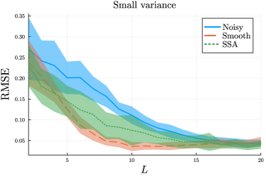
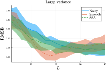
Figure 3: Data preprocessing versus simply using raw noisy data for evaluating self-consistency. The curves show the average RMSE plus/minus the standard deviation over all rollouts.

We revisit the motivating example in Fig. 1: Rollouts with small $L$ are nearly degenerate around the origin. But with additional depth, $L$-length trajectories carry more of a “trend”, hence becoming more distinguishable from noise and improving prediction accuracy. For this example, we consider the system $\frac{1}{s^{2}+0.5s+1}$, discretized with a sampling time of $0.1$ seconds. We assume a standard normal probing signal and output noise with variance $0.1$.

We repeatedly run Section 2 as follows to gauge its prediction accuracy: For a fixed $L$, the initial trajectory is set to the origin in $\mathbb{R}^{2L}$. Then for each ${N\in\{150,200,250\}}$, $10$ rollouts are performed under the same input sequence used in the Hankel matrix. Each rollout uses a new sampled dataset to construct the Hankel matrices. Finally, the RMSE is calculated based on the rollout output trajectory and the true, noise-free underlying signal inside the dataset. These RMSE values are averaged, giving the results shown in Fig. 3. We repeat this experiment with a noise variance of $1.0$ and ${N\in\{1500,2500,5000\}}$.

The curves in Fig. 3 illustrates the RMSE as a function of $L$. We repeat the above procedure using $3$ preprocessing steps of varying complexity:

• Do nothing: This is referred to as “Noisy” and corresponds to using the raw sampled data.

• Smoothing: This is referred to as “Smooth” and corresponds to replacing the measured input–output data with a moving average:

  $$\left\{u_{t},y_{t}\right\}_{t=L-1}^{N-1}\leftarrow\left\{\frac{1}{L}\sum_{k=t-L+1}^{t}u_{k},\frac{1}{L}\sum_{k=t-L+1}^{t}y_{k}\right\}_{t=L-1}^{N-1}$$ (15)

  $L$ serves both as the depth parameter of the Hankel matrix and the moving average window length. With no noise, this is a realizable trajectory, as it corresponds to averaging the internal state sequence. When multiplying the resulting averaged Hankel matrix by some $\alpha$, this strategy is effectively an ensemble of time-shifted noisy Hankel matrices.

• SSA (Hassani, 2007): SSA is a time series analysis method similar to PCA with the key feature of preserving the Hankel structure. Since a reconstructed matrix with the top $L$ singular values/vectors is not necessarily a Hankel matrix, SSA “Hankelizes” it through skew-diagonal averaging, thereby recovering a new signal.

All three preprocessing methods lead to a steep descent in RMSE with respect to $L$. Smoothing the data has the most dramatic descent, both with small and large output noise. However, the error starts to increase after depth $20$ in the right plot of Fig. 3: While Eq. 15 decreases the variance of the output noise, it also decreases the magnitude of the input excitation; moreover, this strategy essentially removes $L$ additional columns from the model (relative to the other methods), tampering with the $L-N$ balance alluded to in Section 3.1. SSA is also a reasonable option in both cases. However, in the large variance setting, it is nearly indistinguishable from the “Noisy” strategy since a large $L$ corresponds to recreating the noise.

In all cases, the simple act of increasing the depth from a fixed dataset has a dramatic positive effect on rollout performance. This is true even without any preprocessing, as illustrated in Fig. 1. However, there are only incremental gains after a certain point. The next example shows that finding the beginning of this plateau is also useful for control.

5.2 Application to LQR

We formulate the LQR problem over the space of trajectories and study the influence of depth on closed-loop performance. Starting with the standard linear equation$\begin{bmatrix}H_{L}(u)\\ H_{L}(y)\end{bmatrix}\alpha=\begin{bmatrix}\overline{u}\\ \overline{y}\end{bmatrix},$ we note that by sequentially applying new inputs $\widehat{u}$, Section 2 relates the current solution vector $\alpha$ to the solution at the next time step $\alpha^{\prime}$ as follows:

$$\left[\begin{array}[]{c}H_{L}(u)\\ H_{L}(y)\end{array}\right]\alpha^{\prime}=\left[\begin{array}[]{c}H^{\prime}_{L-1}(u)\\ \hline\cr 0\\ \hline\cr H^{\prime}_{L}(y)\end{array}\right]\alpha+\left[\begin{array}[]{c}0\\ \hline\cr 1\\ \hline\cr 0\end{array}\right]\widehat{u}=\left[\begin{array}[]{c}\overline{u}_{0:L-2}\\ \hline\cr\widehat{u}\\ \hline\cr\overline{y}^{\prime}\end{array}\right].$$ (16)

That is, Eq. 16 describes the evolution from $\overline{u},\overline{y}$ to $\overline{u}^{\prime},\overline{y}^{\prime}$.

Standard LQR solvers can be readily applied to the trajectory-space model in Eq. 16. In particular, assuming a pseudoinverse solution, one obtains a feedback controller of the form $u=-K\alpha,$ which can be rewritten as

$$u=-K\left[\begin{array}[]{c}H_{L}(u)\\ H_{L}(y)\end{array}\right]^{+}\begin{bmatrix}\overline{u}\\ \overline{y}\end{bmatrix}.$$ (17)

This feedback controller only uses previous input-output data, rather than employing explicit state estimation, to perform actions. We deploy this idea for setpoint tracking on the plant

$$P(z)=0.1159\frac{z^{3}+0.5z}{z^{4}-2.2z^{3}+2.42z^{2}-1.87z+0.7225}$$ (18)

studied by Ljung (1999); Pillonetto and De Nicolao (2010); Yin et al. (2020). Integral action is achieved by defining a state-space model around the variable $x=\begin{bmatrix}\alpha^{\prime}-\alpha\\ r-y\end{bmatrix},$ where $r$ is a reference signal, and solving for the optimal gain matrix. (See, for example, Young and Willems (1972).)

We collect $400$ input-output samples from $P$ with standard normal input and output noise. Some of these samples are shown in Fig. 4. This collection of data is used to run the self-consistency test from Section 5.1. $L=10$ is a minimal yet expressive depth, as it marks the beginning of a plateau akin to that in Fig. 3. To illustrate this, we perform $3$ LQR experiments with $L=5,10,20$. Figure 4 shows that $L=10$ deviates the least from the ground-truth closed-loop trajectory.

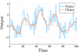
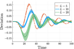
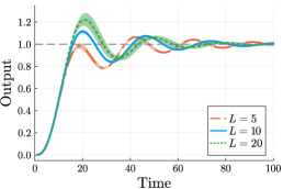
Figure 4: (left) Noisy output data; (center) The difference between the closed-loop trajectory from using a noisy model to obtain LQR controller and the noise-free counterpart; (right) Tracking performance of the noisy controller on the true system.

6 Conclusion

We have illustrated the effectiveness of deep Hankel matrices for approximation and control. In particular, we showed that the length of an input-output trajectory is important for asymptotic approximation properties, while depth influences the transient behavior of this rate. Practically, for a long rollout of excitation data, simply reconfiguring the Hankel matrices for a parsimonious depth has a profound impact on performance. However, we caution that this would not hold in other settings, such as with an impulse response. Therefore, future work should study different probing profiles and extend these results to systems with static nonlinearities or time-varying elements.

Proof of Eq. 7

Inventing the special bold font notation for row vectors with $N-L+1$ consecutive components

$$\bm{z}_{i}=\begin{bmatrix}z_{i}&z_{i+1}&\ldots&z_{i+N-L}\end{bmatrix},\qquad i=0,1,\ldots,L-1$$ (19)

gives the following convenient notation for the $L\times L$ Gram matrix that often appears in what follows: $H_{L}H_{L}^{\top}=\left[\langle\bm{z}_{i},\bm{z}_{j}\rangle\right]_{i,j=1:L}$ where $H_{L}=H_{L}(z)$. Let $z_{0},z_{1},\ldots,$ be a sequence of IID standard normal random variables. Fix $N\geq L$; for convenience, let $\widehat{N}=N-L+1$ denote the number of components in the row vectors $\bm{z}_{i}$ defined in Eq. 19.

We are interested in the set of nonnegative $\sigma$ for which $H_{L}H_{L}^{\top}v=\sigma^{2}v$ for some real-valued vector $v\neq 0$, or equivalently written in Eq. 8. This generalized eigenvalue problem is suitable for a Gershgorin-type argument by containing all $\frac{1}{\sigma^{2}}$ in a set of disks around the origin. In particular, we utilize Corollary $2.6$ in Nakatsukasa (2011): By formulating conditions under which $H_{L}H_{L}^{\top}$ is diagonally dominant, it follows that all $\frac{1}{\sigma^{2}}$ are captured by the union of $L$ disks:

$$\frac{1}{\sigma^{2}}\in\bigcup_{i=0}^{L-1}\left\{s\in\mathbb{C}\colon\lvert s-c_{i}\rvert\leq\rho_{i}\right\},$$ (20)

where the centers and radii are defined by $c_{i}=\frac{1}{\langle\bm{z}_{i},\bm{z}_{i}\rangle}$ and $\rho_{i}=\frac{r_{i}}{\langle\bm{z}_{i},\bm{z}_{i}\rangle(1-r_{i})}$, respectively, with $r_{i}=\frac{1}{\langle\bm{z}_{i},\bm{z}_{i}\rangle}\sum_{j\neq i}\lvert\langle\bm{z}_{i},\bm{z}_{j}\rangle\rvert$ for $i=0,\ldots,L-1$.

To harness this fact, fix any constants $\beta,\gamma$ in $(0,1)$ and introduce

$$\theta=\frac{\gamma(1-\beta)\widehat{N}}{L-1},\quad\text{so}\quad 0\leq(L-1)\theta=\gamma(1-\beta)\widehat{N}.$$ (21)

Consider the random event in which all of the following inequalities hold:

$$\lvert\langle\bm{z}_{i},\bm{z}_{i}\rangle-\widehat{N}\rvert\leq\beta\widehat{N}, i=0,1,\ldots,L-1;$$ (22)

$$\lvert\langle\bm{z}_{i},\bm{z}_{j}\rangle\rvert\leq\theta, i,j=0,1,\ldots,L-1\ \text{with}\ i\neq j.$$ (23)

These conditions suffice to make $H_{L}H_{L}^{\top}$ strictly diagonally dominant, because (for each $i$)

$$\langle\bm{z}_{i},\bm{z}_{i}\rangle\geq\widehat{N}-\beta\widehat{N}=\gamma^{-1}(L-1)\theta>\sum_{j\neq i}\lvert\langle\bm{z}_{j},\bm{z}_{i}\rangle\rvert.$$ (24)

For each $i$, inequality Eq. 23 and definition Eq. 21 imply $r_{i}\leq\frac{(L-1)\theta}{\widehat{N}(1-\beta)}=\gamma.$ We have the bound on the center and radius

$$\lvert c_{i}\rvert\leq\frac{1}{\widehat{N}(1-\beta)}\qquad\text{and}\qquad\rho_{i}\leq\frac{\gamma}{\widehat{N}(1-\beta)(1-\gamma)}.$$ (25)

Applying Eq. 20 for the disks with indices $i=0,\ldots,L-1$, this implies

$$\frac{1}{\sigma^{2}}\leq\lvert c_{i}\rvert+\rho_{i}\leq\frac{1}{\widehat{N}(1-\beta)}\left(1+\frac{\gamma}{1-\gamma}\right).$$ (26)

Therefore, the right side of Eq. 26 converges to $0$ as $N\to\infty$. Define $\epsilon_{N}$ by equating $\epsilon_{N}$ with the right side of Eq. 26. Then Eq. 26 says precisely that $\rho\left(\left(H_{L}H_{L}^{\top}\right)^{-1}\right)\leq\epsilon_{N}$, and we have just shown that $\epsilon_{N}\to 0$ as $N\to\infty$. To complete the proof, it remains only to estimate the probabilities of the random events in Eqs. 22 and 23 in terms of $N$.

This is a consequence of the Hanson-Wright inequality (Rudelson and Vershynin, 2013), which establishes the existence of a universal constant $c>0$ such that

$$\mathbb{P}\left(\lvert z^{\top}Mz-\mathbb{E}\left[z^{\top}Mz\right]\rvert>t\right)\leq 2\exp\left(-c\min\left\{\frac{t^{2}}{\lVert M\rVert_{F}^{2}},\frac{t}{\lVert M\rVert}\right\}\right),\qquad t\geq 0.$$ (27)

for any matrix $M$ Indeed, consider the $\widehat{N}$-dimensional row vectors $\bm{z}_{i}$, $i=0,\ldots,L$. Each one can be extracted from the extra-long row $z=[z_{0}\ \ldots\ z_{N}]$ by multiplication with a suitable block-structured matrix: $\bm{z}_{i}=zU_{i}$ where $U_{i}=\begin{bmatrix}0\\ I\\ 0\end{bmatrix}$ has $i$ zeros in the top block, $L-i$ zeros in the bottom block, and $I\in\mathbb{R}^{\widehat{N}\times\widehat{N}}$. Thus we have $\langle\bm{z}_{i},\bm{z}_{j}\rangle=\bm{z}_{i}{\bm{z}_{j}}^{\top}=zU_{i}{U_{j}}^{\top}z^{\top}.$ Each $M_{ij}=U_{i}{U_{j}}^{\top}$ is a zero matrix of size $(N+1)\times(N+1)$ containing an embedded $\widehat{N}\times\widehat{N}$ identity matrix. The embedding puts the $\widehat{N}$ nonzero elements of matrix $M_{ij}$ on the diagonal if and only if $i=j$. Thus we have $\mathbb{E}\left(zM_{ii}z^{\top}\right)=\widehat{N}$ for $0\leq i\leq L$, and $\mathbb{E}\left(zM_{ij}z^{\top}\right)=0$ whenever $i\neq j$. Now Eq. 27 gives

$$\mathbb{P}\left(\lvert\langle\bm{z}_{i},\bm{z}_{i}\rangle-\widehat{N}\rvert\leq\beta\widehat{N}\right) \geq 1-2\exp\left(-c\beta^{2}\widehat{N}\right) \to 1 0\leq i\leq L-1,$$ (28)

$$\mathbb{P}\left(\lvert\langle\bm{z}_{i},\bm{z}_{j}\rangle\rvert\leq\theta\right) \geq 1-2\exp\left(-c\frac{\gamma^{2}(1-\beta)^{2}\widehat{N}}{(L-1)^{2}}\right) \to 1 i\neq j,\ 0\leq i,j\leq L-1.$$ (29)

In summary, by choosing $N$ sufficiently large, Eqs. 22 and 23 define $L^{2}$ random events that hold with probability arbitrarily close to $1$. $\square$

We gratefully acknowledge the financial support of the Natural Sciences and Engineering Research Council of Canada (NSERC) and Honeywell Connected Plant. We would also like to thank Professor Yaniv Plan for helpful discussions.

References

- Berberich et al. (2021) Julian Berberich, Johannes Köhler, Matthias A. Müller, and Frank Allgöwer. Data-driven model predictive control: Closed-loop guarantees and experimental results. at - Automatisierungstechnik, 69(7):608–618, 2021. 10.1515/auto-2021-0024.
- Berberich et al. (2023) Julian Berberich, Carsten W. Scherer, and Frank Allgöwer. Combining Prior Knowledge and Data for Robust Controller Design. IEEE Transactions on Automatic Control, 68(8):4618–4633, 2023. 10.1109/TAC.2022.3209342.
- Breschi et al. (2023) Valentina Breschi, Alessandro Chiuso, and Simone Formentin. Data-driven predictive control in a stochastic setting: A unified framework. Automatica, 152:110961, 2023. 10.1016/j.automatica.2023.110961.
- Coulson et al. (2019) Jeremy Coulson, John Lygeros, and Florian Dorfler. Data-Enabled Predictive Control: In the Shallows of the DeePC. In 2019 18th European Control Conference (ECC), pages 307–312, Naples, Italy, 2019. IEEE. 10.23919/ECC.2019.8795639.
- Coulson et al. (2023) Jeremy Coulson, Henk J. Van Waarde, John Lygeros, and Florian Dorfler. A Quantitative Notion of Persistency of Excitation and the Robust Fundamental Lemma. IEEE Control Systems Letters, 7:1243–1248, 2023. 10.1109/LCSYS.2022.3232303.
- De Persis and Tesi (2020) Claudio De Persis and Pietro Tesi. Formulas for Data-Driven Control: Stabilization, Optimality, and Robustness. IEEE Transactions on Automatic Control, 65(3):909–924, 2020. 10.1109/TAC.2019.2959924.
- Faulwasser et al. (2023) Timm Faulwasser, Ruchuan Ou, Guanru Pan, Philipp Schmitz, and Karl Worthmann. Behavioral theory for stochastic systems? A data-driven journey from Willems to Wiener and back again. Annual Reviews in Control, 55:92–117, 2023. 10.1016/j.arcontrol.2023.03.005.
- Guo et al. (2023) Baiwei Guo, Yuning Jiang, Colin N. Jones, and Giancarlo Ferrari-Trecate. Data-Driven Robust Control Using Prediction Error Bounds Based on Perturbation Analysis, 2023.
- Hassani (2007) Hossein Hassani. Singular spectrum analysis: Methodology and comparison. Journal of Data Science, 5:239–257, 2007.
- Horn and Johnson (2012) Roger A. Horn and Charles R. Johnson. Matrix Analysis. Cambridge University Press, Cambridge ; New York, 2nd ed edition, 2012.
- Huang et al. (2019) Linbin Huang, Jeremy Coulson, John Lygeros, and Florian Dorfler. Data-Enabled Predictive Control for Grid-Connected Power Converters. In 2019 IEEE 58th Conference on Decision and Control (CDC), pages 8130–8135. IEEE, 2019. 10.1109/CDC40024.2019.9029522.
- Lawrence et al. (2024) Nathan P. Lawrence, Philip D. Loewen, Shuyuan Wang, Michael G. Forbes, and R. Bhushan Gopaluni. Stabilizing reinforcement learning control: A modular framework for optimizing over all stable behavior. Automatica, 164:111642, 2024. https://doi.org/10.1016/j.automatica.2024.111642.
- Ljung (1999) Lennart Ljung. Model Validation and Model Error Modeling. Linköping University Electronic Press, 1999.
- Markovsky and Dörfler (2021) Ivan Markovsky and Florian Dörfler. Behavioral systems theory in data-driven analysis, signal processing, and control. Annual Reviews in Control, page S1367578821000754, 2021. 10.1016/j.arcontrol.2021.09.005.
- Markovsky and Rapisarda (2008) Ivan Markovsky and Paolo Rapisarda. Data-driven simulation and control. International Journal of Control, 81(12):1946–1959, 2008. 10.1080/00207170801942170.
- Markovsky et al. (2006) Ivan Markovsky, Jan C Willems, Sabine Van Huffel, and Bart De Moor. Exact and Approximate Modeling of Linear Systems: A Behavioral Approach. SIAM, 2006.
- Martin et al. (2023) Tim Martin, Thomas B. Schön, and Frank Allgöwer. Guarantees for data-driven control of nonlinear systems using semidefinite programming: A survey. Annual Reviews in Control, 56:100911, 2023. 10.1016/j.arcontrol.2023.100911.
- Nakatsukasa (2011) Yuji Nakatsukasa. Gerschgorin’s theorem for generalized eigenvalue problems in the Euclidean metric. Mathematics of Computation, 80(276):2127–2142, 2011. 10.1090/S0025-5718-2011-02482-8.
- Padoan et al. (2022) Alberto Padoan, Jeremy Coulson, Henk J Van Waarde, John Lygeros, and Florian Dörfler. Behavioral uncertainty quantification for data-driven control. In 2022 IEEE 61st Conference on Decision and Control (CDC), pages 4726–4731. IEEE, 2022.
- Pan et al. (2021) Guanru Pan, Ruchuan Ou, and Timm Faulwasser. On a Stochastic Fundamental Lemma and Its Use for Data-Driven MPC. arXiv:2111.13636, 2021. URL \urlhttp://arxiv.org/abs/2111.13636.
- Pillonetto and De Nicolao (2010) Gianluigi Pillonetto and Giuseppe De Nicolao. A new kernel-based approach for linear system identification. Automatica, 46(1):81–93, 2010. 10.1016/j.automatica.2009.10.031.
- Rudelson and Vershynin (2013) Mark Rudelson and Roman Vershynin. Hanson-Wright inequality and sub-Gaussian concentration. Electronic Communications in Probability, 18(none), 2013. 10.1214/ECP.v18-2865.
- van Waarde et al. (2020) Henk J. van Waarde, Claudio De Persis, M. Kanat Camlibel, and Pietro Tesi. Willems’ fundamental lemma for state-space systems and its extension to multiple datasets. IEEE Control Systems Letters, 4(3):602–607, 2020. 10.1109/LCSYS.2020.2986991.
- van Waarde et al. (2021) Henk J. van Waarde, M. Kanat Camlibel, and Mehran Mesbahi. From noisy data to feedback controllers: Non-conservative design via a matrix S-lemma. IEEE Transactions on Automatic Control, pages 1–1, 2021. 10.1109/TAC.2020.3047577.
- van Waarde et al. (2023) Henk J. van Waarde, Jaap Eising, M. Kanat Camlibel, and Harry L. Trentelman. The informativity approach to data-driven analysis and control, 2023. URL \urlhttp://arxiv.org/abs/2302.10488.
- Willems et al. (2005) Jan C. Willems, Paolo Rapisarda, Ivan Markovsky, and Bart L.M. De Moor. A note on persistency of excitation. Systems & Control Letters, 54(4):325–329, 2005. 10.1016/j.sysconle.2004.09.003.
- Yan et al. (2023) Yitao Yan, Jie Bao, and Biao Huang. On Approximation of System Behavior from Large Noisy Data Using Statistical Properties of Measurement Noise. IEEE Transactions on Automatic Control, pages 1–8, 2023. 10.1109/TAC.2023.3305191.
- Yin et al. (2020) Mingzhou Yin, Andrea Iannelli, and Roy S. Smith. Maximum Likelihood Estimation in Data-Driven Modeling and Control. arXiv:2011.00925 [cs, eess], 2020. URL \urlhttp://arxiv.org/abs/2011.00925.
- Yin et al. (2023) Mingzhou Yin, Andrea Iannelli, and Roy S. Smith. Stochastic Data-Driven Predictive Control: Regularization, Estimation, and Constraint Tightening, 2023.
- Young and Willems (1972) P. C. Young and J. C. Willems. An approach to the linear multivariable servomechanism problem. International Journal of Control, 15(5):961–979, 1972. 10.1080/00207177208932211.