Supplementary Materials for Metric3D v2: A Versatile Monocular Geometric Foundation Model for Zero-shot Metric Depth and Surface Normal Estimation

1 Details for Models

Details for ConvNet models. In our work, our encoder employs the ConvNext [liu2022convnet] networks, whose pretrained weight is from the official released ImageNet-22k pretraining. The decoder follows the adabins [bhat2021adabins]. We set the depth bins number to 256, and the depth range is $[0.3m,150m]$ . We establish 4 flip connections from different levels of encoder blocks to the decoder to merge more low-level features. An hourglass subnetwork is attached to the head of the decoders to enhance background predictions.

Details for ViT models. We use dino-v2 transformers [oquab2023dinov2] with registers [darcet2023vision] as our encoders, which are pretrained on a curated dataset with 142M images. DPT [ranftl2021vision] is used as the decoders. For the ViT-S and ViT-L variants, the DPT decoders take only the last-layer normalized encoder features as the input for stabilized training. The giant ViT-g model instead takes varying-layer features, the same as the original DPT settings. Different from the convnets models above, we use depth bins ranging from $[0.1m,200m]$ for ViT models.

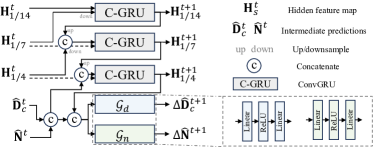
Refer to caption — Figure 1: Detailed structure of the update block. Inspired by RAFTStereo [lipson2021raft], we build slow-fast ConvGRU sub-blocks (denoted as ‘C-GRU’) to refine hierarchical hidden feature maps. Projection heads $\mathcal{G}_{d},\mathcal{G}_{n}$ are attached to the end of the final ConvGRU to prediction update items for the predictions.

Details for recurrent blocks. As illustrated in Fig 1. Each recurrent block updates hierarchical features maps $\{\mathbf{H}^{t}_{1/14},\mathbf{H}^{t}_{1/7},\mathbf{H}^{t}_{1/4}\}$ at $\{\frac{1}{14},\frac{1}{7},\frac{1}{4}\}$ scales and the intermediate predictions s $\hat{\mathbf{D}}_{c}^{t}$ , $\hat{\mathbf{N}}^{t}$ at each iteration step $t$ . This block compromises three ConvGRU sub-blocks to refine feature maps at different scales, and two projection heads $\mathcal{G}_{d}$ and $\mathcal{G}_{n}$ to predict updates for depth and normal respectively. The feature maps are gradually refined from the coarsest ( $\mathbf{H}^{t}_{1/14}$ ) to the finest ( $\mathbf{H}^{t}_{1/4}$ ). For instance, the refined feature map at the $\frac{1}{14}$ scale $\mathbf{H}^{t+1}_{1/14}$ is fed into the second ConvGRU sub-block to refine the $\frac{1}{7}$ -scale feature map $\mathbf{H}^{t}_{1/7}$ . Finally, the projection heads $\mathcal{G}_{d},\mathcal{G}_{n}$ employs a concatenation of original predictions $\hat{\mathbf{D}}_{c}^{t}$ , $\hat{\mathbf{N}}^{t}$ and the to finest feature map $\mathbf{H}^{t}_{1/4}$ to predict the update items $\Delta\hat{\mathbf{D}}_{c}^{t+1}$ , $\Delta\hat{\mathbf{N}}^{t+1}$ . Both projection heads are composed of two linear layers with a sandwiched ReLU activation layer.

Resource comparison of different models. We compare the resource and performance among our model families in Tab. 1. All inference-time and GPU memory results are computed on an Nvida-A100 40G GPU with the original pytorch implemented models (No engineering optimization like TensorRT or ONNX). Generally, the enormous ViT-Large/giant-backbone models enjoy better performance, while the others are more deployment-friendly. In addition, our models built in classical en-decoder schemes run much faster than the recent diffusion counterpart [ke2023repurposing].

Table 1: Comparative analysis of resource and performance across our model families includes evaluation of resource utilization metrics such as inference speed, memory usage, and the proportion of optimization modules. Additionally, we assess metric depth performance on KITTI/NYU datasets and normal performance on NYUv2 dataset, with results derived from checkpoints without fine-tuning. For ViT models, inference speed is measured using 16-bit precision (Bfloat16), which is the same precision as the training setup.

Model			Resource			KITTI Depth		NYUv2 Depth		NYUv2 Normal
Encoder	Decoder	Optim.	Speed	GPU Memory	Optim. time	AbsRel $\downarrow$	$\delta_{1}$ $\uparrow$	AbsRel $\downarrow$	$\delta_{1}$ $\uparrow$	Median $\downarrow$	$30^{\circ}$ $\uparrow$
Marigold[ke2023repurposing] VAE+U-net	U-net+VAE	-	0.13 fps	17.3G	-	No metric	No metric	No metric	No metric	-	-
Ours ConvNeXt-Large	Hourglass	-	10.5 fps	4.2G	-	0.053	0.965	0.083	0.944	-	-
Ours ViT-Small	DPT	4 steps	11.6 fps	2.9G	3.4%	0.070	0.937	0.084	0.945	7.7	0.870
Ours ViT-Large	DPT	8 steps	9.5 fps	7.0G	9.5%	0.052	0.974	0.063	0.975	7.0	0.881
Ours ViT-giant	DPT	8 steps	5.0 fps	15.6G	25%	0.051	0.977	0.067	0.980	7.1	0.881

Table 2: Training and testing datasets used for experiments.

Datasets	Scenes	Source	Label	Size	#Cam.
Training Data
DDAD [packnet]	Outdoor	Real-world	Depth	$\sim$ 80K	36+
Lyft [lyftl5preception]	Outdoor	Real-world	Depth	$\sim$ 50K	6+
Driving Stereo (DS) [yang2019drivingstereo]	Outdoor	Real-world	Depth	$\sim$ 181K	1
DIML [cho2021diml]	Outdoor	Real-world	Depth	$\sim$ 122K	10
Arogoverse2 [Argoverse2]	Outdoor	Real-world	Depth	$\sim$ 3515K	6+
Cityscapes [Cordts2016Cityscapes]	Outdoor	Real-world	Depth	$\sim$ 170K	1
DSEC [Gehrig21ral]	Outdoor	Real-world	Depth	$\sim$ 26K	1
Mapillary PSD [MapillaryPSD]	Outdoor	Real-world	Depth	750K	1000+
Pandaset [itsc21pandaset]	Outdoor	Real-world	Depth	$\sim$ 48K	6
UASOL [bauer2019uasol]	Outdoor	Real-world	Depth	$\sim$ 1370K	1
Virtual KITTI [cabon2020virtual]	Outdoor	Synthesized	Depth	37K	2
Waymo [sun2020scalability]	Outdoor	Real-world	Depth	$\sim$ 1M	5
Matterport3d [zamir2018taskonomy]	In/Out	Real-world	Depth + Normal	144K	3
Taskonomy [zamir2018taskonomy]	Indoor	Real-world	Depth + Normal	$\sim$ 4M	$\sim$ 1M
Replica [straub2019replica]	Indoor	Real-world	Depth + Normal	$\sim$ 150K	1
ScanNet^† [dai2017scannet]	Indoor	Real-world	Depth + Normal	$\sim$ 2.5M	1
HM3d [ramakrishnan2021habitat]	Indoor	Real-world	Depth + Normal	$\sim$ 2000K	1
Hypersim [roberts2021hypersim]	Indoor	Synthesized	Depth + Normal	54K	1
Testing Data
NYU [silberman2012indoor]	Indoor	Real-world	Depth+Normal	654	1
KITTI [Geiger2013IJRR]	Outdoor	Real-world	Depth	652	4
ScanNet^† [dai2017scannet]	Indoor	Real-world	Depth+Normal	700	1
NuScenes (NS) [caesar2020nuscenes]	Outdoor	Real-world	Depth	10K	6
ETH3D [schops2017multi]	Outdoor	Real-world	Depth	431	1
DIODE [vasiljevic2019diode]	In/Out	Real-world	Depth	771	1
iBims-1 [koch2018evaluation]	Indoor	Real-world	Depth	100	1

†

ScanNet is a non-zero-shot testing dataset for our ViT models.

1.1 Datasets and Training and Testing

We collect over $16$ M data from 18 public datasets for training. Datasets are listed in Tab. 2. When training the ConvNeXt-backbone models, we use a smaller collection containing the following 11 datasets with $8$ M images: DDAD [packnet], Lyft [lyftl5preception], DrivingStereo [yang2019drivingstereo], DIML [cho2021diml], Argoverse2 [Argoverse2], Cityscapes [Cordts2016Cityscapes], DSEC [Gehrig21ral], Maplillary PSD [MapillaryPSD], Pandaset [itsc21pandaset], UASOL[bauer2019uasol], and Taskonomy [zamir2018taskonomy]. In the autonomous driving datasets, including DDAD [packnet], Lyft [lyftl5preception], DrivingStereo [yang2019drivingstereo], Argoverse2 [Argoverse2], DSEC [Gehrig21ral], and Pandaset [itsc21pandaset], have provided LiDar and camera intrinsic and extrinsic parameters. We project the LiDar to image planes to obtain ground-truth depths. In contrast, Cityscapes [Cordts2016Cityscapes], DIML [cho2021diml], and UASOL [bauer2019uasol] only provide calibrated stereo images. We use raftstereo [lipson2021raft] to achieve pseudo ground-truth depths. Mapillary PSD [MapillaryPSD] dataset provides paired RGB-D, but the depth maps are achieved from a structure-from-motion method. The camera intrinsic parameters are estimated from the SfM. We believe that such achieved metric information is noisy. Thus we do not enforce learning-metric-depth loss on this data, i.e., $L_{silog}$ , to reduce the effect of noises. For the Taskonomy [zamir2018taskonomy] dataset, we follow LeReS [yin2022towards] to obtain the instance planes, which are employed in the pair-wise normal regression loss. During training, we employ the training strategy from [yin2020diversedepth_old] to balance all datasets in each training batch.

The testing data is listed in Tab. 2. All of them are captured by high-quality sensors. In testing, we employ their provided camera intrinsic parameters to perform our proposed canonical space transformation.

1.2 Details for Some Experiments

Finetuning protocols. To finetune the large-scale-data trained models on some specific datasets, we use the ADAM optimizer with the initial learning rate beginning at $10^{-6}$ and linear decayed to $10^{-7}$ within $6$ K steps. Notably, such finetune does not require a large batch size like large-scale training. We use in practice a batch-size of $16$ for the ViT-g model and $32$ for ViT-L. The models will converge quickly in approximately $2$ K steps. To stabilize finetuning, we also leverage the predictions $\tilde{\mathbf{D}}_{c}$ $\tilde{\mathbf{N}}$ of the pre-finetuned model as alternative pseudo labels. These labels can sufficiently impose supervision upon the annotation-absent regions. The complete loss can be formulated as:

\begin{split}L_{ft}=0.01L_{d-n}(\mathbf{D}_{c},\mathbf{N})+L_{d}(\mathbf{D}_{c},\mathbf{D}^{\ast}_{c})+L_{n}(\mathbf{N},\mathbf{N^{\ast}})\\ +0.01(L_{d}(\mathbf{D}_{c},\tilde{\mathbf{D}}_{c})+L_{n}(\mathbf{N},\tilde{\mathbf{N}})),\end{split}

(1)

where $\mathbf{D}_{c}$ and $\mathbf{N}$ are the predicted depth in the canonical space and surface normal, $\mathbf{D}^{\ast}_{c}$ and $\mathbf{N}^{\ast}$ are the groundtruth labels, $L_{d}$ , $L_{n}$ , and $L_{d-n}$ are the losses for depth, normal, and depth-normal consistency introduced in the main text.

Evaluation of zero-shot 3D scene reconstruction. In this experiment, we use all methods’ released models to predict each frame’s depth and use the ground-truth poses and camera intrinsic parameters to reconstruct point clouds. When evaluating the reconstructed point cloud, we employ the iterative closest point (ICP) [besl1992method] algorithm to match the predicted point clouds with ground truth by a pose transformation matrix. Finally, we evaluate the Chamfer $\ell_{1}$ distance and F-score on the point cloud.

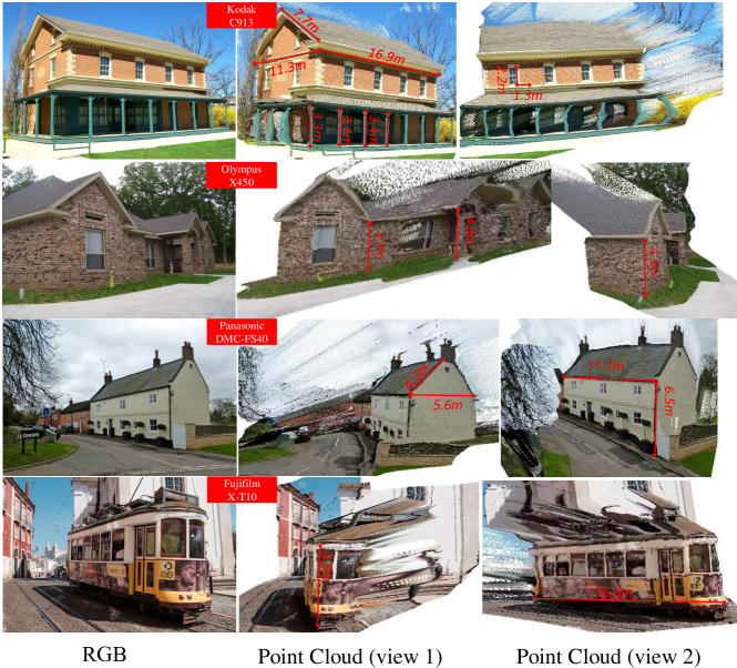
Reconstruction of in-the-wild scenes. We collect several photos from Flickr. From their associated camera metadata, we can obtain the focal length $\hat{f}$ and the pixel size $\delta$ . According to $\nicefrac{{\hat{f}}}{{\delta}}$ , we can obtain the pixel-represented focal length for 3D reconstruction and achieve the metric information. We use meshlab software to measure some structures’ size on point clouds. More visual results are shown in Fig. 6.

Generalization of metric depth estimation. To evaluate our method’s robustness of metric recovery, we test on 7 zero-shot datasets, i.e. NYU, KITTI, DIODE (indoor and outdoor parts), ETH3D, iBims-1, and NuScenes. Details are reported in Tab. 2. We use the officially provided focal length to predict the metric depths. All benchmarks use the same depth model for evaluation. We don’t perform any scale alignment.

Evaluation on affine-invariant depth benchmarks. We follow existing affine-invariant depth estimation methods to evaluate 5 zero-shot datasets. Before evaluation, we employ the least square fitting to align the scale and shift with ground truth [leres]. Previous methods’ performance is cited from their papers.

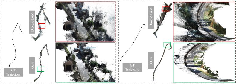
Dense-SLAM Mapping. This experiment is conducted on the KITTI odometry benchmark. We use our model to predict metric depths, and then naively input them to the Droid-SLAM system as an initial depth. We do not perform any finetuning but directly run their released codes on KITTI. With Droid-SLAM predicted poses, we unproject depths to the 3D point clouds and fuse them together to achieve dense metric mapping. More qualitative results are shown in Fig. 5.

1.3 More Visual Results

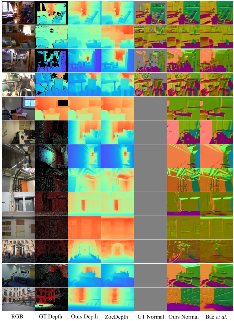
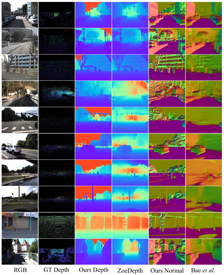
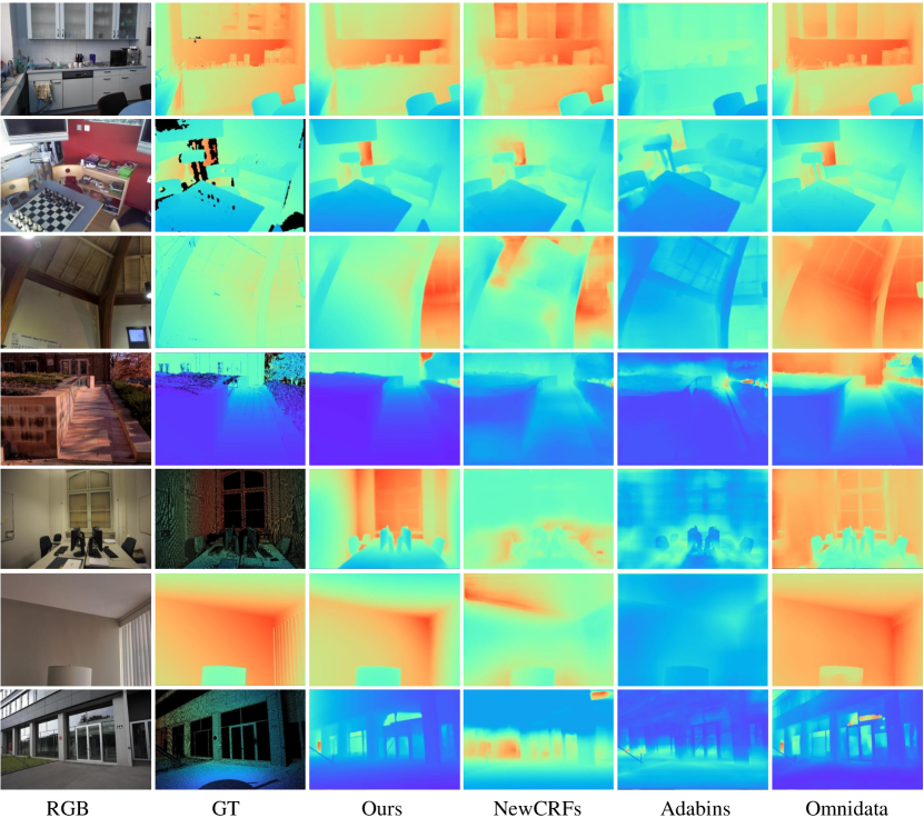
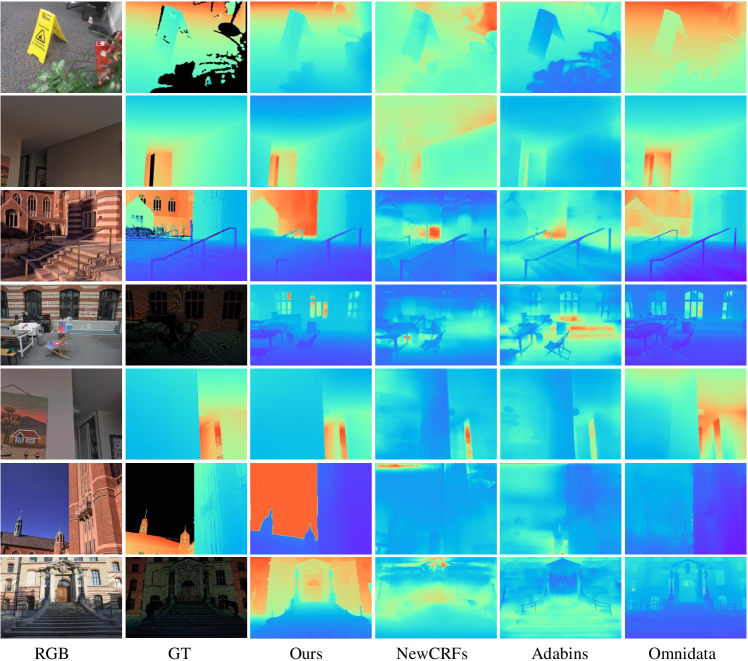
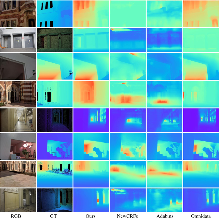
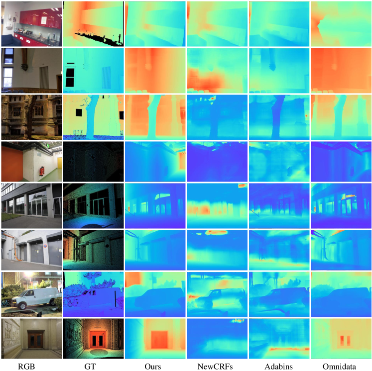
Qualitative comparison of depth and normal estimation. In Figs 2, 3, we compare visualized depth and normal maps from the Vit-g CSTM_label model with ZoeDepth [bhat2023zoedepth], Bae etal [bae2021estimating], and Omnidata [eftekhar2021omnidata]. In Figs. 4, 8, 9, and 10, We show the qualitative comparison of our depth maps from the ConvNeXt-L CSTM_label model with Adabins [bhat2021adabins], NewCRFs [yuan2022new], and Omnidata [eftekhar2021omnidata]. Our results have much fine-grained details and less artifacts.

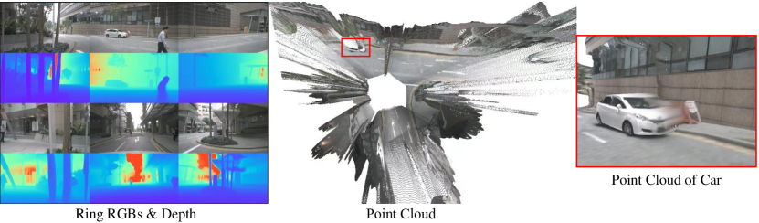
Reconstructing 360^∘ NuScenes scenes. Current autonomous driving cars are equipped with several pin-hole cameras to capture 360^∘ views. Capturing the surround-view depth is important for autonomous driving. We sampled some scenes from the testing data of NuScenes. With our depth model, we can obtain the metric depths for 6-ring cameras. With the provided camera intrinsic and extrinsic parameters, we unproject the depths to the 3D point cloud and merge all views together. See Fig. 7 for details. Note that 6-ring cameras have different camera intrinsic parameters. We can observe that all views’ point clouds can be fused together consistently.