A New Parameterization for Finding Solutions for Microlensing Exoplanet Light Curves
Abstract
The gravitational microlensing method of discovering exoplanets and multi-star systems can produce degenerate solutions, some of which require in-depth analysis to uncover. We propose a new parameter space that can be used to sample potential solutions more efficiently and is more robust at finding all degenerate solutions. We identified two new parameters, and , that can be sampled in place of the mass ratios and separations of the systems under analysis to identify degenerate solutions. The parameter is related to the size of the central caustic, , while is related to the distance of a point along the contour from log()=0, where is the projected planet-host separation. In this work, we present the characteristics of these parameters and the tests we conducted to prove their efficacy.
1 Introduction
Gravitational microlensing is a method used to discover and characterize exoplanets (Liebes, 1964; Mao & Paczynski, 1991). When a “lens” star passes in front of a “source” star relative to our line of sight, the gravity of the lens star bends the light of the source star, leading to a magnification pattern in the light curve of the source star (Einstein, 1936). This pattern changes when the lens is composed of multiple bodies, for example a star hosting one or more planets. The mass ratio(s) of the star and planet(s), , and the separation between the star and planet(s), , can be derived from the magnification pattern in the light curve of such a microlensing event.
In general, the analysis of gravitational microlensing data is conducted by generating model light curves that assume particular characteristics (“parameters”) of the lens and source systems and then using algorithms to fit those models to the observed data by tweaking the parameters of the model. The most commonly used algorithms to conduct fitting involve grid searches, Markov Chain Monte Carlo (MCMC) processes, or some combination of the two.
In the case of some events, multiple degenerate solutions can be found to fit observed data approximately equally as well. One of the earliest known degeneracies was the degeneracy between and solutions (Griest & Safizadeh, 1998). Since then, many others have been encountered, some mathematical in nature and some “accidental” (i.e., due to poor light curve coverage from gaps in the observational data). For example in Bennett et al. (2008), sixteen different potential solution sets were identified for the same microlensing event (MOA-2007-BLG-192) due to the presence of four two-fold degeneracies. Because we cannot tell for sure which degenerate solution is the true solution, an algorithm might be missing the true solution if it misses a degenerate solution. Hence, it is important that all degenerate solutions are identified by the fitting algorithms used to analyze microlensing data.
There are several examples of degenerate solutions being initially overlooked in past research. For example, both microlensing events analyzed in Yang et al. (2022) were found to suffer the “central-resonant” caustic degeneracy, in which it could not be determined whether the caustic that caused the magnification pattern was a central or a resonant caustic. This results in multiple potential values for , as well as other parameters. This degeneracy was not identified in the initial grid search for solutions, and required a denser grid search to be uncovered. A similar situation occurred in the analysis of two events by Ryu et al. (2022). All four events are drawn from a single year (2021), and Yang et al. (2022) notes that this relatively high frequency of occurrence indicates that the degeneracy may have been missed in previous events as well. In fact, once this degeneracy was recognized, re-analysis of OGLE-2016-BLG-1195 led to the discovery of new, previously–un-probed, solutions (Gould et al., 2023). Making grid searches more robust to the “central-resonant” degeneracy is the primary motivation for this work.
Current grid search algorithms most often sample evenly in (log(), log()) space. However, the local minima of microlensing event parameter spaces often follow a v-shaped pattern symmetrical about log() 0. This pattern roughly aligns with the boundaries in log() and log() separating different types of caustics. It might be more efficient to sample a higher density of test points within such a distribution instead of sampling evenly in log() and log(). Sampling within this distribution might identify local minima that would otherwise require a higher-resolution grid search to unearth.
To construct a new grid that samples more densely from the region of interest, we found two new parameters related to and such that, when evenly spaced points in the space of these two new parameters are mapped to (log(), log()) space, they follow a similar distribution pattern as the distribution seen in many microlensing events. In this paper, we describe how we defined these parameters and used them to construct a grid in log() and log() space and the tests we conducted to assess the efficacy of the new grid.
2 New Parameters
2.1 Defining k and h
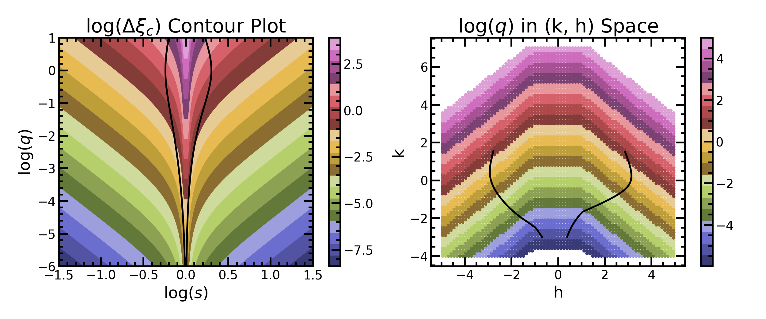
We defined the new parameters based on characteristics of the caustics associated with given values of and , because these caustics change as and change. Our goal was to find a caustic characteristic that changes rapidly in the region of interest (near log()=0 on either side). This characteristic would serve as the first parameter, , and the distance along the contour lines of this parameter would serve as the second, , so that points evenly spaced in these parameters will bunch up and become over-dense in that region when mapped back to log() and log().
We evaluated different caustic characteristics by plotting points in (log(), log()) space with colors corresponding to the value of the caustic characteristic. Ultimately, we determined that the logarithm of the horizontal width of the central caustic, , behaves in the desired manner (Chung et al., 2005):
| (1) |
Previously, Dong et al. (2009) used a similar parameter, (the extent of the central caustic in the y-direction), to conduct a grid search for solutions to MOA-2007-BLG-400. They argued that this parameter would be useful in cases for which it could be estimated directly from the light curve. Here, we use the measurement along the x-axis, which has a simpler analytic form. Similar to the observation by Dong et al. (2009) about , is linear with in many regimes111In fact, (see Eq. 11 and 12 of Chung et al., 2005).. The key to this work, which can be seen in Figure 1, is that it is non-linear as . This property makes an effective search parameter for all cases, even those for which there is no central caustic and those for which it cannot be estimated directly from the light curve.
As shown in Figure 1, contour lines of in (log(), log()) space bunch up in the target region of (log(), log()) space as desired. However, the contours also asymptote as they approach log()=0, which would result in infinitely dense contours as log() approaches 0. Thus, to ensure that is defined at all values of log(), we defined both and as piece-wise functions with different definitions near log()=0. We define a transition point at .
So, for :
| (2) |
For , we hold constant over changing log():
| (3) |
i.e., for each point (log(), log()) within this range, we set equal to the value of at the point .
For the parameter , we want a definition that generally reflects a distance from . For , the contours become approximately straight lines in (, ) space so they may be described as a simple magnitude equation, but this breaks down as because the slope of changes dramatically. Of course, this slope change is the behavior that gets us the higher density of contours for . So, for , we define to maintain the density of points just outside this region.
Hence, for :
| (4) |
where is defined as the value of at which and = the value of at (, ).
For
| (5) |
Finally, for :
| (6) |
where such that the contours match up at . We choose because it maintains the approximate spacing near the transition point.
A grid of points in (, ) space, color-coded by values of log(), can be found in Figure 1.
2.2 Evaluating the New Grid
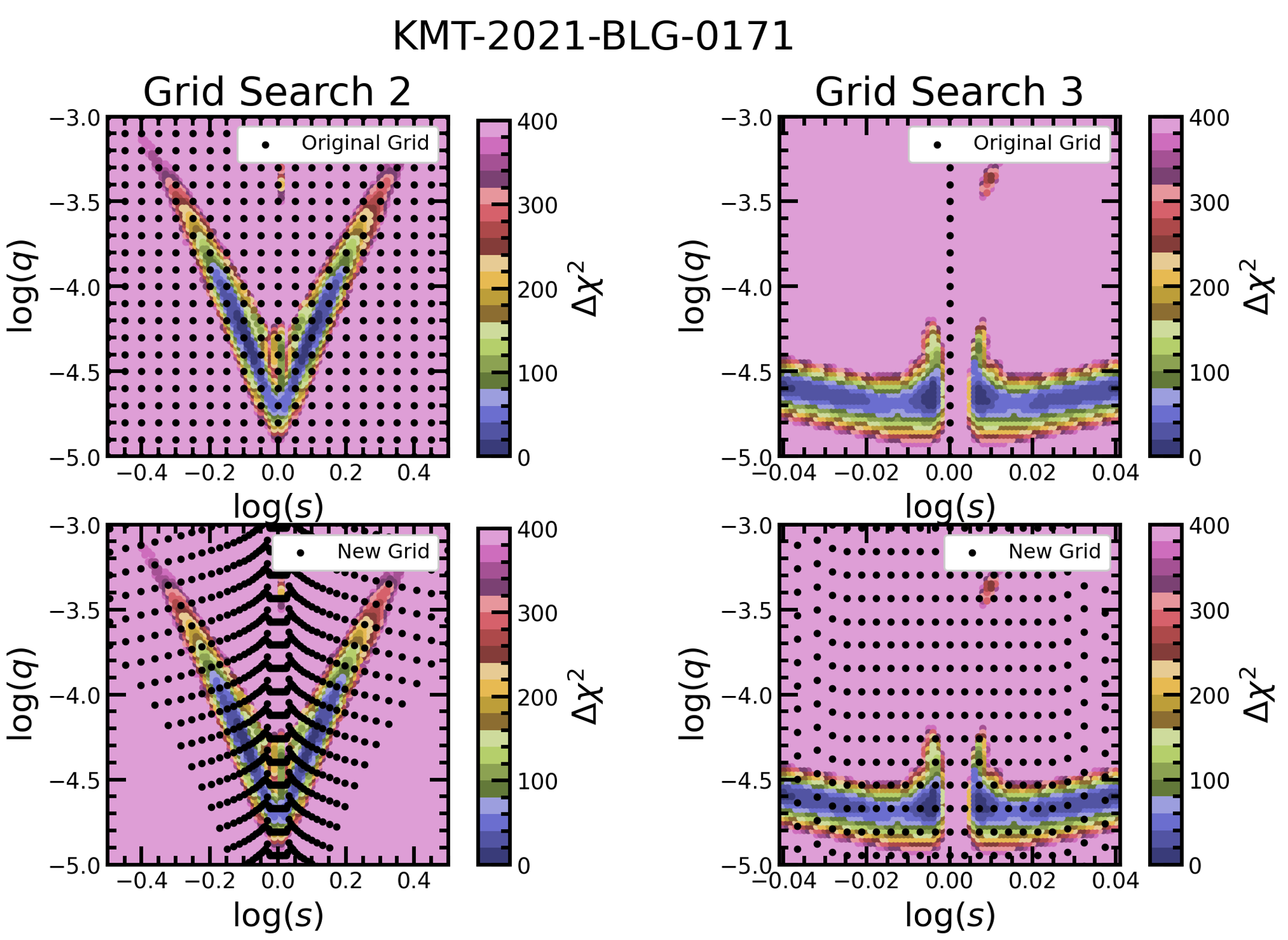
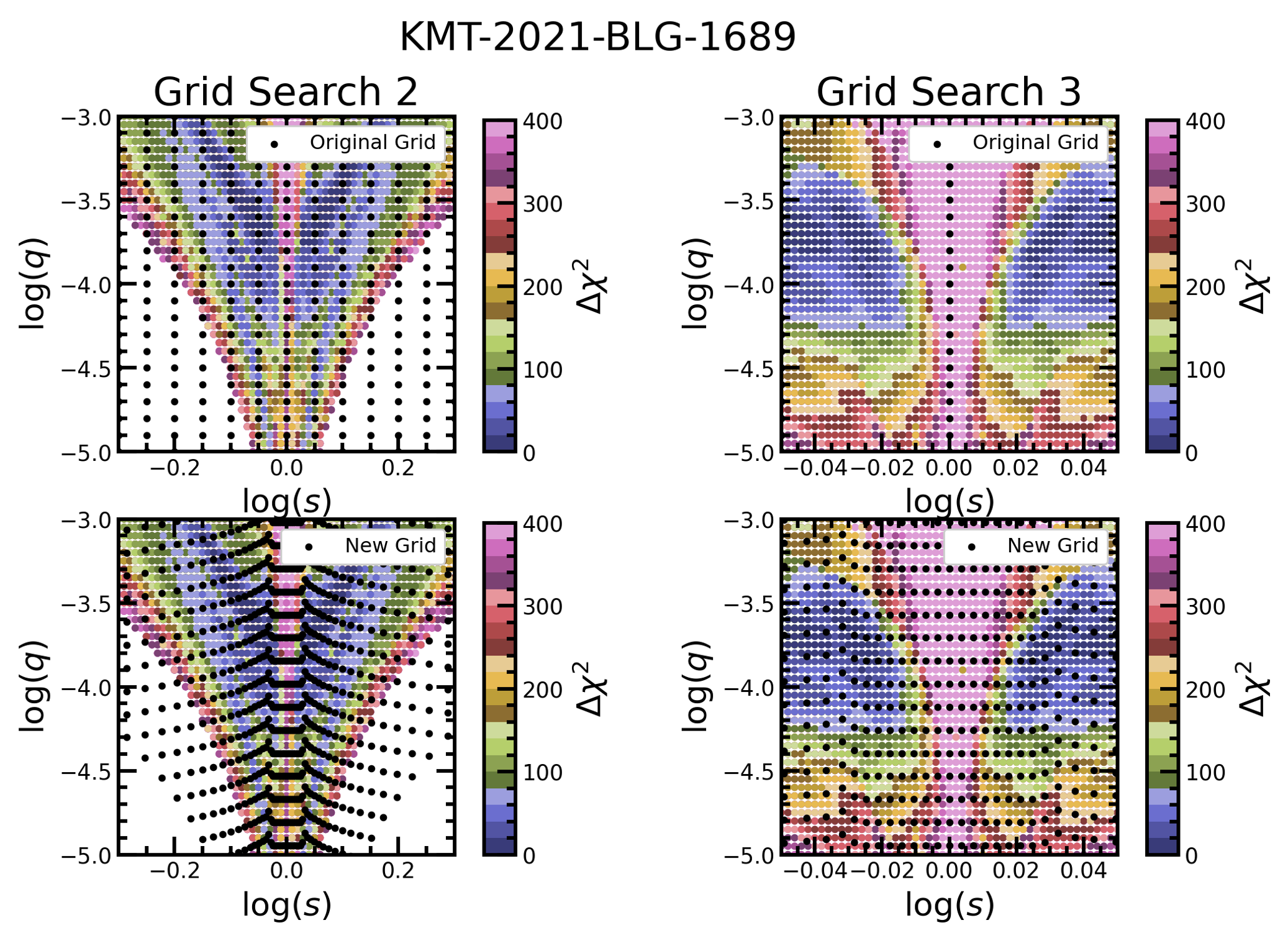
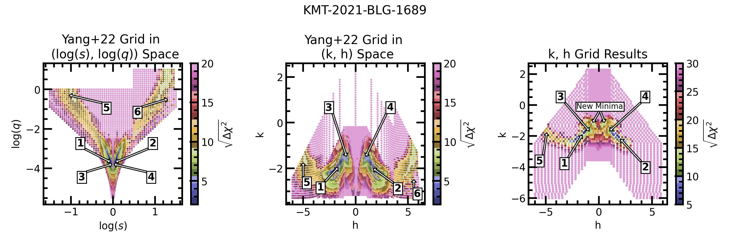
Yang et al. (2022) ultimately needed to perform three grid searches of increasing densities and increasingly narrow parameter ranges in order to uncover all 4 degenerate solutions for KMT-2021-BLG-0171 and all 6 degenerate solutions for KMT-2021-BLG-1689, because their initial grid was not dense enough in the regions where the solutions were located to find all solutions. Therefore, to estimate the efficacy of the new grid, we compared the new grid to the initial (log(), log()) grid employed by Yang et al. (2022) in their analysis of events KMT-2021-BLG-0171 and KMT-2021-BLG-1689.
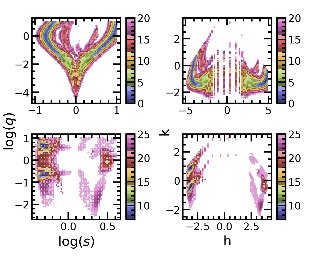
Figures 2 and 3 show both the new grid points and the initial grid search points used by Yang et al. (2022) overlaid on the distributions found by the densest grid searches performed by Yang et al. (2022) for events KMT-2021-BLG-0171 (for which two degenerate pairs of solutions were found) and KMT-2021-BLG-1689 (for which three degenerate pairs of solutions were found). Each of the grids have approximately the same number of total points covering the range between -1.5 1.5 and -6 1 (the new grid has slightly fewer). As can be seen from these plots, the new grid contains many more points within the local minima than the initial grid from Yang et al. (2022), which suggests that the new grid might be better at identifying these minima.
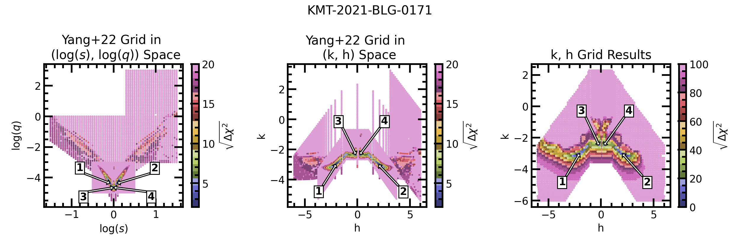
We also investigated the efficacy of the new parameters by calculating (, ) values for the points in the grid searches conducted by Yang et al. (2022) and re-plotting the distribution in (, ) space. These plots can be found in Figure 4. As can be seen in these Figures, the different minima are well-separated in (, ) space, suggesting that a reasonably dense grid of points evenly spaced in and would be able to resolve all of the minima.
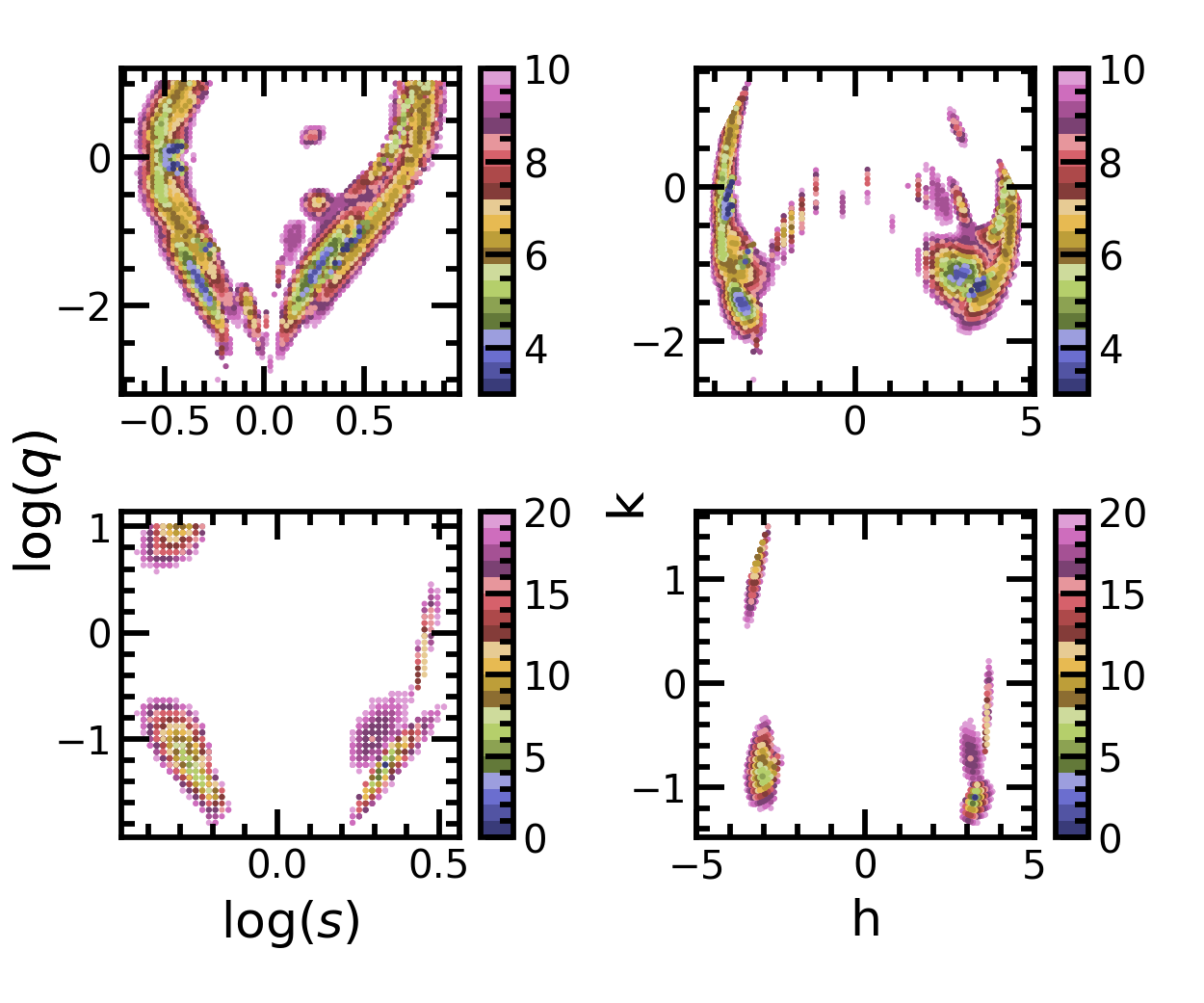
Ideally, this grid would be effective at finding solutions for a variety of microlensing events, not just planetary microlensing events. Thus, to test whether binary star system solutions would be resolvable in (, ) space, we repeated this interpolation process for the distributions found using a (log(), log()) grid for four additional events, all with binary-star-system lens solutions. These events are KMT-2016-BLG-0020, KMT-2016-BLG-0157, KMT-2016-BLG-0199, KMT-2016-BLG-2542. They were chosen from events modeled in the AnomalyFinder (Zang et al., 2021) search for planets in the 2016 prime fields (Shin et al., 2023) and selected for having a variety of morphologies for the surface in (log(), log())-space.
The (log(), log()) grids as well as their transforms into (, )-space can be found in Figures 5 and 6. As can be seen in these figures, all of the minima resolvable in (log(), log()) space are also resolvable in (, ) space. Thus, the (, ) grid should also be effective at analyzing non-planetary events.
3 Tests
In order to prove the efficacy of the new grid, we conducted a grid search/MCMC analysis of three different previously-analyzed microlensing events as case tests: KMT-2021-BLG-0171 and KMT-2021-BLG-1689 (Yang et al., 2022) and MOA-2007-BLG-192 (Bennett et al., 2008). These events each suffer from multiple degeneracies. For each search, we used VBBL (Bozza et al., 2018) with MulensModel (Poleski & Yee, 2019) to generate the light curves and emcee (Foreman-Mackey et al., 2013) to refine the parameters, keeping , , and the source size, , fixed. The following section will describe each event in more detail and present the results of our analysis.
3.1 KMT-2021-BLG-0171
The solutions previously found for this event are listed in Table 1. This event suffers from a degeneracy between the (1, 2) and (3, 4) solutions. Both 1 and 2 predict the same values for source size and , and both 3 and 4 predict the same values for and , but the values predicted by (1, 2) and (3, 4) differ from each other for both parameters. Additionally, (1, 2) predict a larger absolute value for than (3, 4) (known as the “central-resonant” degeneracy). Within each pair, the “close-wide” degeneracy is also present. This is a common microlensing degeneracy where two solutions exist that are identical except that the value for has approximately undergone a transformation. See Griest & Safizadeh (1998) and Dominik (1999) for further discussion of this degeneracy, and see Yang et al. (2022) for more information on this event and its solutions.
The (, ) grid was successful in identifying all four solutions identified by Yang et al. (2022) in a single grid search, in contrast to the three grid searches required in Yang et al. (2022). See Figure 4 for a plot of the distribution from our grid search and Table 1 for a comparison of the solutions found by the (, ) grid and the solutions found by Yang et al. (2022).
| Grid | Solution | t0 (HJD) | u0 | tE (d) | (10-3) | (deg) | (10-5) | |
|---|---|---|---|---|---|---|---|---|
| Yang+22 | 1 | 2459326.2338 | 0.00564 | 41.57 | 1.50 | 237.6 | 0.813 | 4.28 |
| 0.0003 | 0.00005 | 0.32 | 0.015 | 0.7 | 0.032 | 0.80 | ||
| , | 2459326.2344 | 0.00563 | 41.7 | 1.50 | 237.7 | 0.807 | 4.39 | |
| Yang+22 | 2 | 2459326.2338 | 0.00564 | 41.56 | 1.51 | 237.7 | 1.232 | 4.17 |
| 0.0003 | 0.00005 | 0.32 | 0.015 | 0.7 | 0.051 | 0.82 | ||
| , | 2459326.2343 | 0.00559 | 41.9 | 1.50 | 237.6 | 1.240 | 4.39 | |
| Yang+22 | 3 | 2459326.2338 | 0.00565 | 41.57 | 1.62 | 239.1 | 0.9905 | 2.19 |
| 0.0003 | 0.00005 | 0.32 | 0.007 | 0.4 | 0.0009 | 0.14 | ||
| , | 2459326.2340 | 0.00569 | 41.5 | 1.50 | 239.6 | 0.9874 | 1.60 | |
| Yang+22 | 4 | 2459326.2338 | 0.00565 | 41.55 | 1.62 | 239.2 | 1.0161 | 2.22 |
| 0.0003 | 0.00005 | 0.31 | 0.007 | 0.4 | 0.0009 | 0.15 | ||
| , | 2459326.2340 | 0.00563 | 41.7 | 1.50 | 239.2 | 1.0198 | 1.60 |
3.2 KMT-2021-BLG-1689
This event suffers from a degeneracy between the (1, 2) and (3, 4) solutions. The two pairs predict different values for and . This event also suffers from the central-resonant degeneracy between solution pairs (1, 2) and (3, 4), and solution pairs (1, 2), (3, 4), and (5, 6) each suffer from the close-wide degeneracy. See Table 2 and Yang et al. (2022) for more information on this event and its solutions.
The (, ) grid was successful in finding solutions 1 through 5 in a single grid search, compared to the three grid searches used by Yang et al. (2022). It did not find a minimum near the location of solution 6, but that solution has the secondary as the center of magnification, so it is in a completely different (, ) coordinate system. See Figure 4 for a plot of the distribution from this grid search and Table 2 for a comparison of the solutions found by the (, ) grid and the solutions found by Yang et al. (2022).
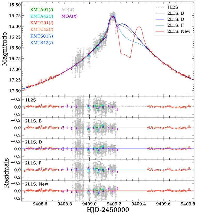
The (, ) grid also appeared to have found two new minima, not previously identified by Yang et al. (2022), that represent a potential new solution suffering from the close-wide degeneracy. We ran a refined MCMC analysis on these minima and found the set of parameters with the best value listed in Table 3, with the corresponding light curve shown in Figure 7. These minima were investigated as potential new solutions but were ultimately rejected due to their high values. However, they are a better fit to the data than the binary solutions (5, 6) investigated in Yang et al. (2022). Thus, the fact that they were discovered by the (, ) grid suggests that this grid has the potential to uncover solutions that would be missed by the traditional (log(), log()) grid.
| Grid | Solution | t0 (HJD) | u0 | tE (d) | (10-3) | (deg) | (10-4) | |
|---|---|---|---|---|---|---|---|---|
| Yang+22 | 1 | 2459409.2510 | 0.00600 | 22.56 | 1.44 | 242.3 | 0.870 | 2.10 |
| 0.0011 | 0.00028 | 0.84 | 0.08 | 0.6 | 0.025 | 0.39 | ||
| 2459409.2525 | 0.00588 | 22.67 | 1.44 | 240.6 | 0.880 | 1.80 | ||
| Yang+22 | 2 | 2459409.2509 | 0.00601 | 22.51 | 1.44 | 242.3 | 1.157 | 2.09 |
| 0.0011 | 0.00026 | 0.79 | 0.08 | 0.6 | 0.032 | 0.37 | ||
| 2459409.2516 | 0.00579 | 23.06 | 1.44 | 241.1 | 1.240 | 2.86 | ||
| Yang+22 | 3 | 2459409.2509 | 0.00590 | 22.61 | 0.70 | 242.1 | 0.944 | 1.62 |
| 0.0012 | 0.00027 | 0.85 | 0.08 | 0.6 | 0.004 | 0.17 | ||
| 2459409.2517 | 0.00599 | 21.65 | 1.44 | 239.5 | 0.941 | 1.04 | ||
| Yang+22 | 4 | 2459409.2510 | 0.00587 | 22.78 | 0.68 | 242.2 | 1.067 | 1.62 |
| 0.0011 | 0.00027 | 0.81 | 0.08 | 0.5 | 0.005 | 0.18 | ||
| 2459409.2534 | -0.00602 | 21.88 | 1.44 | 120.6 | 1.070 | 1.04 | ||
| Yang+22 | 5 | 2459409.2403 | 0.00663 | 22.92 | 1.2 | 340.9 | 0.092 | 5079 |
| 0.0012 | 0.00032 | 0.88 | – | 1.0 | 0.006 | 2232 | ||
| 2459409.2463 | 0.00725 | 21.41 | 1.44 | 155.0 | 0.100 | 3896 | ||
| Yang+22 | 6 | 2459409.2394 | 0.00327 | 46.14 | 0.8 | 160.8 | 19.97 | 3186 |
| 0.0009 | 0.00060 | 8.48 | – | 0.5 | 1.25 | 1979 | ||
| Not Found |
| t0 (HJD) | u0 | tE (d) | (10-3) | (deg) | (10-4) | ||
|---|---|---|---|---|---|---|---|
| 2459409.2493 | 0.00694 | 23.04 | 1.91 | 104.1 | 0.951 | 4.57 | 61.42 |
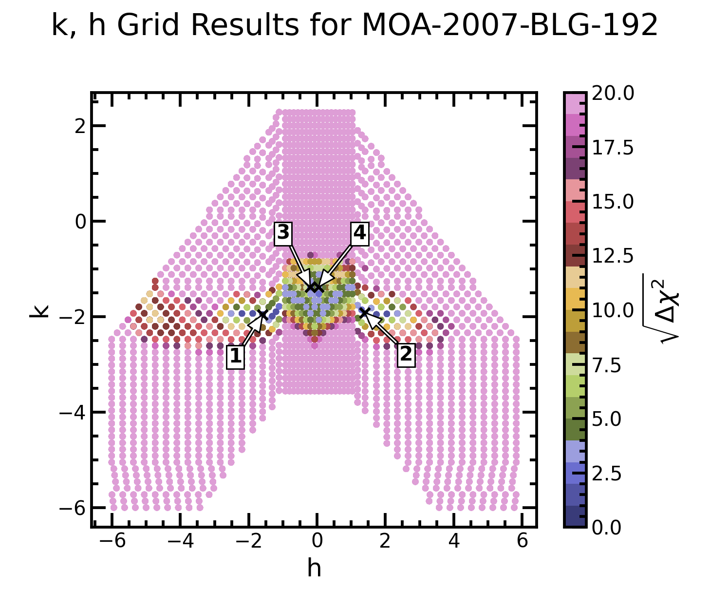
3.3 MOA-2007-BLG-192
Two four-fold degeneracies contribute to the 16 solutions found for this event by Bennett et al. (2008). The most relevant degeneracies for this work are those which produce variation in log() and log() amongst the solutions; one such degeneracy is due to an undersampling of data which led to an inability to distinguish whether a caustic crossing vs. cusp approaching model is superior, and the other is the close-wide degeneracy. We list a few of these solutions in Table 4. This event is also challenging to analyze due to the lack of data coverage of the event. See Bennett et al. (2008) for more information on this event and its solutions.
The () grid was successful in finding solutions 1 and 2 in a single grid search with a fixed value of equal to the value found by Bennett et al. (2008) for solution 1. Although it did not find solutions 3 and 4 given this value of , it did find them when we ran the grid search again with a fixed value of equal to the value found by Bennett et al. (2008) for solution 3. Thus, if had been allowed to vary, a single grid search might have been able to identify all four solutions. See Figure 8 for a plot of the distribution from this grid search and Table 4 for a comparison of the solutions found by the () grid and the solutions found by Bennett et al. (2008).
| Grid | Solution | t0 (HJD) | u0 | tE (d) | (10-4) | (deg) | (10-4) | |
|---|---|---|---|---|---|---|---|---|
| Bennett+08 | 1 | 2454245.453 | -0.00364 | 75.0 | 8.93 | 113.6 | 0.881 | 1.5 |
| 2454245.452 | -0.00406 | 69.1 | 8.93 | 292.5 | 0.880 | 1.8 | ||
| Bennett+08 | 2 | 2454245.453 | -0.00360 | 74.5 | 8.59 | 115.8 | 1.120 | 1.2 |
| 2454245.448 | -0.00387 | 71.7 | 8.93 | 294.5 | 1.109 | 1.3 | ||
| Bennett+08 | 3 | 2454245.462 | -0.00433 | 75.1 | 15.6 | 101.1 | 0.985 | 2.1 |
| 2454245.458 | -0.00480 | 66.0 | 15.6 | -76.44 | 0.987 | 2.0 | ||
| Bennett+08 | 4 | 2454245.458 | -0.00420 | 74.9 | 15.2 | 103.8 | 1.007 | 1.6 |
| 2454245.451 | -0.00476 | 66.9 | 15.6 | 282.4 | 1.003 | 2.0 |
4 Summary
Our goal in this work was to increase the analytic sensitivity of gravitational microlensing parameter searches by creating a grid search method more sensitive to the degenerate solutions observed in Yang et al. (2022). We accomplished this goal by sampling points to be tested as solutions in a new parameter space that requires a lower density of points to be able to identify solutions compared to parameter spaces more commonly used. We defined these parameters by looking for caustic characteristics that change rapidly in the regions of (log(), log()) space where degenerate solutions where more likely to be located, so that grid points sampled evenly in these parameters would be more likely to pick up on solutions. We ultimately defined these parameters based on the width of the central caustic of a given event. We tested a grid sampled evenly in these new parameters, which we name and , on three events with degenerate solutions and found that the new grid could more efficiently identify most if not all of the solutions identified by previous analyses. We thus present the and parameters as a potential new tool to be used in the analysis of gravitational microlensing events in the future. Given that this tool is more sensitive to the central-resonant degeneracy, it provides the opportunity for increased automation and efficiency in the analysis of gravitational microlensing events. This will be especially important for microlensing searches with the Roman Space Telescope.
J.C.Y. and I.-G.S. acknowledge support from U.S. NSF Grant No. AST-2108414. This research has made use of publicly available data (https://kmtnet.kasi.re.kr/ulens/) from the KMTNet system operated by the Korea Astronomy and Space Science Institute (KASI) at three host sites of CTIO in Chile, SAAO in South Africa, and SSO in Australia. Data transfer from the host site to KASI was supported by the Korea Research Environment Open NETwork (KREONET). The computations in this paper were conducted on the Smithsonian High Performance Cluster (SI/HPC), Smithsonian Institution. https://doi.org/10.25572/SIHPC.
References
- Bennett et al. (2008) Bennett, D., Bond, I., Udalski, A., et al. 2008, The Astrophysical Journal, 684, 663
- Bozza et al. (2018) Bozza, V., Bachelet, E., Bartolić, F., et al. 2018, Monthly Notices of the Royal Astronomical Society, 479, 5157
- Chung et al. (2005) Chung, S.-J., Han, C., Park, B.-G., et al. 2005, The Astrophysical Journal, 630, 535
- Dominik (1999) Dominik, M. 1999, arXiv preprint astro-ph/9903014
- Dong et al. (2009) Dong, S., Bond, I. A., Gould, A., et al. 2009, ApJ, 698, 1826, doi: 10.1088/0004-637X/698/2/1826
- Einstein (1936) Einstein, A. 1936, Science, 84, 506, doi: 10.1126/science.84.2188.506
- Foreman-Mackey et al. (2013) Foreman-Mackey, D., Hogg, D. W., Lang, D., & Goodman, J. 2013, PASP, 125, 306, doi: 10.1086/670067
- Gould et al. (2023) Gould, A., Shvartzvald, Y., Zhang, J., et al. 2023, AJ, 166, 145, doi: 10.3847/1538-3881/aced3c
- Griest & Safizadeh (1998) Griest, K., & Safizadeh, N. 1998, The Astrophysical Journal, 500, 37
- Liebes (1964) Liebes, S. 1964, Physical Review, 133, 835, doi: 10.1103/PhysRev.133.B835
- Mao & Paczynski (1991) Mao, S., & Paczynski, B. 1991, The Astrophysical Journal, 374, L37
- Poleski & Yee (2019) Poleski, R., & Yee, J. C. 2019, Astronomy and computing, 26, 35
- Ryu et al. (2022) Ryu, Y.-H., Jung, Y. K., Yang, H., et al. 2022, arXiv preprint arXiv:2202.03022
- Shin et al. (2023) Shin, I.-G., Yee, J. C., Zang, W., et al. 2023, AJ, 166, 104, doi: 10.3847/1538-3881/ace96d
- Yang et al. (2022) Yang, H., Zang, W., Gould, A., et al. 2022, Monthly Notices of the Royal Astronomical Society, 516, 1894
- Zang et al. (2021) Zang, W., Hwang, K.-H., Udalski, A., et al. 2021, AJ, 162, 163, doi: 10.3847/1538-3881/ac12d4