Abstract

The supersymmetric analysis of spinning cosmic string spacetime, involving an electron in magnetic fields, has been conducted. We examined the Dirac system within extended special functions known as exceptional orthogonal polynomials. Corresponding Dirac system is transformed to a relativistic system with a nonlinear isotonic oscillator. Furthermore, new potential models that extend the radial oscillator by adding rational terms are expressed in terms of the exceptional orthogonal Laguerre $X_{m}$ polynomial. The necessary analyses of the potential, energy levels, and probability density graphs are introduced for various cosmic string topological defects and Aharonov-Bohm interaction parameters.

, $a$ is the rotation parameter given in terms of angular momentum $J$, $a=4J$. The interval for the parameters can be written as $-\infty<z<\infty$, $r\geq 0$, $0\leq\varphi\leq 2\pi$. The metric is proposed as [24]

$$ds^{2}=dt^{2}+2adtd\varphi-(\alpha^{2}r^{2}-a^{2})d\varphi^{2}-dr^{2}-dz^{2},$$ (2)

where the $\alpha^{2}r^{2}-a^{2}<0$ a condition related to closed timelike curves [27], [28], the spacetime admits closed timelike curves if $r<\frac{|a|}{\alpha}$. The dynamics equation for a spin-$1/2$ particle, considering its interaction with rotation and external magnetic fields, is given by

$$i\gamma^{\mu}(x)(\nabla_{\mu}+ieA_{\mu}(x))\Psi(x)=M\Psi(x),$$ (3)

where covariant derivaive is $\nabla_{\mu}=\partial_{\mu}+\Gamma_{\mu}$. Dirac matrices $\gamma^{\mu}(x)$ satisfy the expression

$$\gamma^{\mu}(x)=e_{a}^{\mu}(x)\gamma^{a},$$ (4)

where $e^{\mu}_{a}$ are the tetrad fields, $\gamma^{a}$ are the flat matrices in Minkowski spacetime where

$$\gamma^{0}=\left(\begin{array}[]{cc}1&0\\ 0&-1\\ \end{array}\right),~{}~{}\gamma^{i}=\left(\begin{array}[]{cc}0&\sigma^{i}\\ \sigma^{i}&0\\ \end{array}\right).$$ (5)

The anti-commutation of the Dirac matrices give metric tensor, i.e.

$$\{\gamma^{\mu}(x),\gamma^{\nu}(x)\}=2g^{\mu\nu}(x).$$ (6)

In the covariant derivative definition, the spin affine connection reads as

$$\Gamma_{\mu}(x)=\frac{1}{4}\gamma^{a}\gamma^{b}e^{\mu}_{a}(x)(\partial_{\mu}e_{b\nu}(x)-\Gamma^{\sigma}_{\mu\nu}e_{b\sigma}(x)),$$ (7)

where $\Gamma^{\sigma}_{\mu\nu}$ are the Christoffel symbols. It is understood that tetrads are coefficients of components of an orthogonal basis, and the metric tensor can be transformed from a coordinate basis to the tetrad basis. Here, the tetrad basis is used as follows,

$$e^{a}_{\mu}(x)=\left(\begin{array}[]{cccc}1&0&a&0\\ 0&\cos\varphi&-r\alpha\sin\varphi&0\\ 0&\sin\varphi&r\alpha\cos\varphi&0\\ 0&0&0&1\\ \end{array}\right),~{}~{}e^{\mu}_{a}(x)=\left(\begin{array}[]{cccc}1&\frac{a\sin\varphi}{r\alpha}&-\frac{a\cos\alpha}{r\alpha}&0\\ 0&\cos\varphi&\sin\varphi&0\\ 0&-\frac{\sin\varphi}{r\alpha}&\frac{\cos\varphi}{r\alpha}&0\\ 0&0&0&1\\ .\end{array}\right)$$ (8)

Then, spinor affine connection reads as

$$\Gamma_{\mu}=(0,0,\frac{i}{2}(1-\alpha)\Sigma,0)$$ (9)

where

$$\Sigma=\left(\begin{array}[]{cccc}1&0&0&0\\ 0&-1&0&0\\ 0&0&1&0\\ 0&0&0&-1\\ \end{array}\right).$$ (10)

Because (3) includes magnetic field interactions, vector potential can be expressed as

A $$= [0,A_{\varphi},0]$$ (11)

$$A_{\varphi}(r) = -\frac{1}{2}\alpha Br^{2}-\frac{\Phi}{e}$$ (12)

where $\Phi$ is the magnetic flux through the solenoid. In the presence of A, as given in (11), the wavefunction of an electron is influenced by this vector potential, even the magnetic field $\textbf{B}=\nabla\times\textbf{A}=B_{z}\hat{k}$ is zero. $A_{\varphi}(r)$, exhibiting cylindrical symmetry, would affect the particle’s wavefunction in a manner similar to that in an electron-nucleus system. Therefore, the Aharonov-Bohm phenomenon is expected to occur around the cosmic string considered in this study. Next, the spinor of the fermion field is written as below

$$\Psi(t,r,\varphi)=\exp(-iEt)\left(\begin{array}[]{c}\psi_{1}(r,\varphi)\\ \psi_{2}(r,\varphi)\\ \end{array}\right)$$ (13)

where

$$\psi_{1}(r,\varphi) = \left(\begin{array}[]{c}e^{im\varphi}\psi_{11}(r)\\ ie^{i(m+1)\varphi}\psi_{12}(r)\\ \end{array}\right),~{}~{}~{}~{}\psi_{2}(r,\varphi)=\left(\begin{array}[]{c}e^{im\varphi}\psi_{21}(r)\\ ie^{i(m+1)\varphi}\psi_{22}(r)\\ \end{array}\right)$$ (18)

Then, the Dirac system is separated as follows,

$$-\frac{1}{2M}u^{\prime\prime}_{11}+\left(\frac{\ell_{1}(\ell_{1}+1)}{2Mr^{2}}+V_{1}(r)\right)u_{11}(r) = \varepsilon^{2}u_{11}(r)$$ (19)

$$-\frac{1}{2M}u^{\prime\prime}_{12}+\left(\frac{\ell_{2}(\ell_{2}+1)}{2Mr^{2}}+V_{2}(r)\right)u_{12}(r) = \varepsilon^{2}u_{12}(r)$$ (20)

where $\varepsilon^{2}=E^{2}-M^{2}$ and,

$$V_{1}(r) = \frac{B^{2}e^{2}}{8M}r^{2}-\frac{Be}{2M}\left(\ell_{1}+\frac{3}{2}\right)$$ (21)

$$V_{2}(r) = \frac{B^{2}e^{2}}{8M}r^{2}-\frac{Be}{2M}\left(\ell_{2}+\frac{1}{2}\right).$$ (22)

Here, wavefunction transformations and angular momentum numbers are defined as follows,

$$u_{1i}(r) = \sqrt{r}\psi_{1i}(r),~{}~{}i=1,2,$$ (23)

$$\ell_{1} = \frac{1+2m-2\alpha+2aE-2\Phi}{2\alpha},$$ (24)

$$\ell_{2} = \frac{-1-2m-2\alpha-2aE+2\Phi}{2\alpha}.$$ (25)

The system defined by equations (19) and (20), with the elements given in (21) and (22), is known as a three-dimensional oscillator. The solutions to this system are already known. So, the system, as presented in [29], reads as follows

$$-y^{\prime\prime}(x)+V_{\ell}(x)y(x)=\epsilon y(x)$$ (26)

$$V_{\ell}(x)=\frac{1}{4}\omega^{2}x^{2}+\frac{\ell(\ell+1)}{x^{2}},$$ (27)

and the solutions are given by [29]

$$\epsilon^{\ell}_{n}=\omega\left(2n+\ell+\frac{3}{2}\right),~{}~{}~{}~{}n=0,1,2,...$$ (28)

$$y_{n}(x)=\left(\frac{\omega}{2}\right)^{\frac{1}{2}(\ell+3/2)}\sqrt{\frac{2n!}{\Gamma(n+\ell+3/2)}}~{}x^{\ell+1}e^{-\frac{1}{4}\omega x^{2}}L^{\ell+1/2}_{n}\left(\frac{1}{2}\omega x^{2}\right),$$ (29)

where $L^{\ell+1/2}_{n}(\frac{1}{2}\omega x^{2})$ are the Laguerre polynomials. Now we can define (19) and (20) in terms of the new variable of $x$ which is $x=\sqrt{2M}r$ and obtain ,

$$-u^{\prime\prime}_{11}(x)+V_{eff}(x)u_{11}(x) = \epsilon^{2}u_{11}(x)$$ (30)

$$-u^{\prime\prime}_{12}(x)+U_{eff}(x)u_{12}(x) = \epsilon^{2}u_{12}(x),$$ (31)

and

$$V_{eff}(x) = \frac{\ell_{1}(\ell_{1}+1)}{x^{2}}+\frac{B^{2}e^{2}}{16M^{2}}x^{2}-\frac{Be}{2M}\left(\ell_{1}+\frac{3}{2}\right),$$ (32)

$$U_{eff}(x) = \frac{\ell_{2}(\ell_{2}+1)}{x^{2}}+\frac{B^{2}e^{2}}{16M^{2}}x^{2}-\frac{Be}{2M}\left(\ell_{2}+\frac{1}{2}\right)$$ (33)

If we match (26) and (19), we obtain the parameters $\{\omega,\ell\}$ in terms of our parameters as

$$\omega = \frac{Be}{2M}$$ (34)

$$\ell = \ell_{1}~{}~{}~{}~{}or~{}~{}~{}~{}\ell=-1-\ell_{1}.$$ (35)

By the way, $\ell_{2}$ can be obtained from $\ell_{1}$ using the mirror symmetry of the parameters $E,m,\Phi$, i.e,

$$E\rightarrow-E,~{}~{}m\rightarrow-m,~{}~{}\Phi\rightarrow-\Phi.$$ (36)

Then, we can express $E_{n}$ and $u^{\ell_{1}}_{11,n}(r)$ given as below

$$E^{\ell_{1}}_{n} = \frac{-aBe}{2M\alpha}\pm\frac{\sqrt{4a^{2}B^{2}e^{2}-8M\alpha\gamma}}{4M\alpha},~{}~{}\ell=-1-\ell_{1}$$ (37)

where $\gamma=Be(1+2m-\alpha-2n\alpha-2\Phi)-2M^{3}\alpha$,

$$u^{\ell}_{11,n}(x)=\left(\frac{Be}{2M}\right)^{\frac{1}{2}(\ell_{1}+3/2)}\sqrt{\frac{2n!}{\Gamma(n+\ell_{1}+3/2)}}~{}x^{\ell_{1}+1}e^{-\frac{1}{4}\frac{Be}{2M}x^{2}}L^{\ell_{1}+1/2}_{n}\left(\frac{Be}{4M}x^{2}\right).$$ (38)

Here, (19) and (20) are known as shape invariant potentials in the literature [30]. In the standard SUSY QM, the superpotential is given in terms of the derivative of the groundstate solutions $W(r)=-\frac{u^{\prime}_{11,0}(x)}{u_{11,0}(x)}$ and the partner potentials are expressed using the function $W(x)$,

$$V_{eff}(x)=V_{1}(x) = W^{2}(x)-\frac{dW}{dx}+E^{2}$$ (39)

$$V_{2}(x) = W^{2}(x)+\frac{dW}{dx}+E^{2}.$$ (40)

If we call the Hamiltonian operator for each system in (19) and (20) as

$$H_{1} = \mathcal{A}^{{\dagger}}\mathcal{A}=-\frac{d^{2}}{dx^{2}}+V_{1}(x)-E^{2}$$ (41)

$$H_{2} = \mathcal{A}\mathcal{A}^{{\dagger}}=-\frac{d^{2}}{dx^{2}}+V_{2}(x)-E^{2}$$ (42)

and

$$\mathcal{A}=\frac{d}{dx}+W(x),~{}~{}\mathcal{A}^{{\dagger}}=-\frac{d}{dx}+W(x)$$ (43)

where $E$ is the factorization energy,  $\mathcal{A}u_{11,0}(x)=0$, $u_{11,0}(x)$ is the groundstate wavefunction of the corresponding $V_{1}(x)$ potential. Here, $V_{2}(x)$ shares the same energy spectrum with $V_{1}(x)$ except groundstate [30]. We can define now the superpotential as

$$W(x)=\frac{Be}{4M}x+\frac{\ell_{1}}{x},$$ (44)

where we use the second solution to the angular momentum $\ell=-\ell_{1}-1$. Hence, we can continue with the extension of the radial oscillator classes of our system. Before, let’s check the graph of potential functions and energy levels.

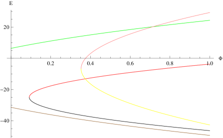
Figure 1: Energy levels given in 37 with respect to parameter $\Phi$. $M=2,m=1,e=1,n=1$ for each curve while $(B,a,\alpha)=(100,0.1,0.1),(1,0.5,0.2),(8,0.1,0.45)$ for red/black, green/brown and for pink and yellow curves.

In Figure $1$, it is observed that as the $\alpha$ topological deflection parameter with the angular momentum parameter $a$ increase, the energy levels become less negative.

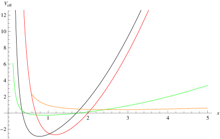
Figure 2: Effective potential graph of (32)$M=2,m=1,e=1,B=10,\alpha=0.5$ for each curve while $(\Phi,a)=(0.4,1),(5.0,2),(10,5),(20,2)$ for red, black, green and orange correspondingly.

Figure 2 shows that for smaller values of the magnetic flux parameter $\Phi$, the equilibrium point of the potential appears deeper. When $\Phi$ assumes dramatically greater values, the potential curve approaches zero more rapidly.

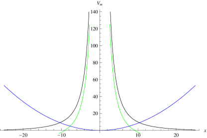
Figure 3: Effective potential graph of (33)$M=2,m=1,e=1,n=1,\Phi=0.10,\alpha=0.1$ for each curve while ${(B,a)}={(0.1,1.2),(0.5,10),(140,50)}$ for black, green and blue curves correspondingly.

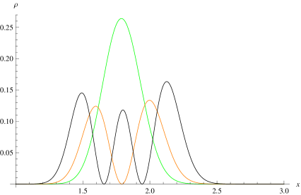
Figure 4: Probability density $\rho(r)=|u_{11}|^{2}+|u_{12}|^{2}$ graphs where $u_{12}$ are the solutions of (31). $B=100,\alpha=0.1,\Phi=10,a=0.1$ and n=0,1,2 for green, orange and black curves correspondingly.

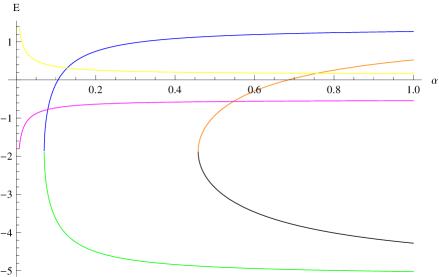
Figure 5: Energy levels given in 37 with respect to parameter $\alpha$. $M=2,m=1,e=1,a=0.1$ for each curve while $(\Phi,B)=(0.5,5),(1.3,10),(5.0,50)$ for orange/black, blue/green and for yellow/magenta curves respectively.

The topological deflection parameter is increased to $\alpha=0.9$ in Figure 3, which depicts the partner potential graph of (33). As observed in the graph, as $B$ and $\alpha$ increase, the potential well becomes deeper. Figure $4$ shows the probability density graph is drawn for the solutions given in (38).

In figure $5$, as the value of $\alpha$ increases, the energy becomes more stable.

2.1 Rationally extended radial oscillator model

ansatz for the superpotential
Let us give an ansatz for the superpotential which may both give $V_{1}(x)$ in (39) under some parameter restrictions and also produce the partner potential $V_{2,p}(x)$ which is different from the one given in (40). Then, we have

$$W(x)=\frac{a_{1}}{x}+a_{2}x-\frac{f^{\prime}(x)}{f(x)}.$$ (45)

This ansatz in (45) is given in [29], then, we can follow the straightforward algebra in [29]. Thus, one obtains $V_{1}(x)$ and $V_{2,p}(x)$ as follows

$$V_{1}(x) = a_{2}(2a_{1}-1)+\frac{a_{1}(a_{1}+1)}{x^{2}}+a^{2}_{2}x^{2}+\frac{2a_{1}f^{\prime}(x)}{f(x)}+\frac{2a_{2}xf^{\prime}(x)}{f(x)}+\frac{2f^{\prime 2}}{f^{2}}-\frac{f^{\prime\prime}}{f}$$ (46)

$$V_{2,p}(x) = a_{2}(2a_{1}+1)+\frac{a_{1}(a_{1}-1)}{x^{2}}+a^{2}_{2}x^{2}+\frac{2a_{1}f^{\prime}(x)}{f(x)}+\frac{2a_{2}xf^{\prime}(x)}{f(x)}+\frac{2f^{\prime 2}}{f^{2}}+\frac{f^{\prime\prime}}{f}.$$ (47)

Using (45) in (39) and (40) and $f(x)=x^{2}+c$, one gets

$$V_{1}(x)=E^{2}+2a_{1}a_{2}-a_{2}+\frac{a_{1}(a_{1}+1)}{x^{2}}+a^{2}_{2}x^{2}-\frac{4a_{2}x^{2}+4a_{1}-2}{c+x^{2}},$$ (48)

$$V_{2,p}(x)=E^{2}+2a_{1}a_{2}+a_{2}+\frac{a_{1}(a_{1}-1)}{x^{2}}+a^{2}_{2}x^{2}-\frac{4a_{2}x^{2}+4a_{1}+2}{c+x^{2}}+\frac{8x^{2}}{(c+x^{2})^{2}}.$$ (49)

We can eliminate the rational and constant terms in (48) using the parameters

$$c=\frac{2a_{1}-1}{2a_{2}},~{}~{}E^{2}=-a_{2}(2a_{1}-5).$$ (50)

Then, $V_{2,p}(x)$ is obtained as

$$V_{2,p}(x)=V_{1}(x)+2W^{\prime}(x)=a^{2}_{2}x^{2}+\frac{a_{1}(a_{1}-1)}{x^{2}}+\frac{4}{x^{2}+c}-\frac{8c}{(x^{2}+c)^{2}}+2a_{2},$$ (51)

where

$$a_{1}(a_{1}-1)=\ell_{1}(\ell_{1}+1),~{}~{}~{}~{}a^{2}_{2}=\frac{B^{2}e^{2}}{16M^{2}}.$$ (52)

The solutions are given by $\{(a_{1},a_{2})=(-\ell_{1},\frac{Be}{4M}),(-\ell_{1},-\frac{Be}{4M}),(1+\ell_{1},\frac{Be}{4M}),(1+\ell_{1},-\frac{Be}{4M})\}$. Next, we can focus on the solutions of (51). In the literature, (51) is known as quantum isotonic nonlinear-oscillator potentials [31], [32]. It is noted that (51) can be compared to Eq.$(28)$ in [31]. If we apply the supersymmetric relationship of the wavefunctions

$$u_{12}(x)=C_{2}\mathcal{A}^{{\dagger}}u_{11}=C_{2}\left(-\frac{d}{dx}+\frac{\ell_{1}+1}{x}+\frac{Be}{4M}x-\frac{2x}{x^{2}+c}\right)u_{11}(x)$$ (53)

where $u_{11}(x)$ is given by (38). Using the differential identity of Laguerre polynomials given below

$$\frac{d}{dz}L^{\alpha}_{n}(z)=-L^{\alpha+1}_{n-1}(z),$$ (54)

and

$$L^{\alpha}_{n}(z)=L^{\alpha}_{n-1}+L^{\alpha-1}_{n}(z),$$ (55)

we obtain

$$u_{12}(x)=C_{2}\frac{x^{\ell_{1}+2}e^{-\frac{Bex^{2}}{8M}}}{x^{2}+c^{2}}\left((2\ell_{1}+2n+5)L^{\ell_{1}+1/2}_{n}(x^{\prime})-2(n+1)L^{\ell_{1}+1/2}_{n+1}(x^{\prime})+\frac{Bec^{2}}{4M}L^{\ell_{1}+3/2}_{n}(x^{\prime})\right)$$ (56)

where $x^{\prime}=\frac{Be}{4M}x^{2}$.
Figure $6$ is drawn for (51) which also shows that a potential well can be obtained for the smaller values of $\Phi$. Upon examining Figure $7$ it is seen that the rationally extended potential in equation (74) differs from those shown previously. For smaller $\Phi$ values, such as $\Phi=0.1$ there is singularity at the points $|x|=7.797$. Figure $8$ presents the probability densities for the solutions given in equations (33) and (56) while Figure $8$ shows the probability densities for the solutions given in equations $V_{{}_{\textbf{m}}}(x)$ and (56).

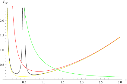
Figure 6: Effective partner potential $V_{2,p}(x)$ graphs. $\Phi=0.5,1.5,0.1,50$ corresponding to black, yellow,red, green curves.

3 Exceptional Orthogonal Polynomials

3.1 $X_{\textbf{m}}$ exceptional Laguerre polynomials

$X_{1}$-Jacobi and $X_{1}$- Laguerre are known as exceptional orthogonal polynomials which exist as two infinite sequences of polynomial eigenfunctions of a Sturm–Liouville problem. Unlike the classical orthogonal polynomial systems, their sequences start with a polynomial of degree one. These polynomials $R(g(x))$ satisfy a second order differential equation which is given by

$$R^{\prime\prime}(g(x))+F(g)R^{\prime}(g(x))+G(g)R(g(x))=0.$$ (57)

Here, $F(g)$ and $G(g)$ functions are given as

$$F(g) = \frac{1}{g}\left((\alpha^{\prime}+1-g)-2g\frac{L^{\alpha^{\prime}}_{\textbf{m}-1}(-g)}{L^{\alpha^{\prime}-1}_{\textbf{m}}}(-g)\right)$$ (58)

$$G(g) = \frac{1}{g}\left(n-2\alpha^{\prime}\frac{L^{\alpha^{\prime}}_{\textbf{m}-1}(-g)}{L^{\alpha^{\prime}-1}_{\textbf{m}}(-g)}\right),~{}~{}\textbf{m}\geq 0,~{}~{}n\geq\textbf{m},~{}~{}\alpha^{\prime}>0.$$ (59)

The norm integral is given by

$$\int^{\infty}_{0}(L^{\alpha^{\prime}}_{n,\textbf{m}}(g))^{2}W^{\alpha^{\prime}}_{\textbf{m}}(g)dg=\frac{(\alpha^{\prime}+n)\Gamma(\alpha^{\prime}+n+\textbf{m})}{(n-\textbf{m})!},$$ (60)

where

$$W^{\alpha^{\prime}}_{n}(g)=\frac{g^{\alpha^{\prime}}e^{-g}}{(L^{\alpha^{\prime}-1}_{\textbf{m}})^{2}}$$ (61)

and $X_{m}$ Laguerre polynomials can be written as

$$L^{\alpha^{\prime}}_{n,\textbf{m}}=L^{\alpha^{\prime}}_{\textbf{m}}(-g)L^{\alpha^{\prime}-1}_{n-\textbf{m}}+L^{\alpha^{\prime}-1}_{\textbf{m}}(-g)L^{\alpha^{\prime}}_{n-\textbf{m}-1},~{}~{}n\geq\textbf{m}.$$ (62)

$X_{m}$-exceptional orthogonal Laguerre polynomials satisfies the differential equation below

$$\frac{d^{2}L^{\alpha^{\prime}}_{n,\textbf{m}}}{dx^{2}}+\frac{1}{g}\left((\alpha^{\prime}+1-g)-2g\frac{L^{\alpha^{\prime}}_{\textbf{m}-1}(-g)}{L^{\alpha^{\prime}-1}_{\textbf{m}}(-g)}\right)\frac{dL^{\alpha^{\prime}}_{n,\textbf{m}}(g)}{dx}+\frac{1}{g}\left(n-2\alpha^{\prime}\frac{L^{\alpha^{\prime}}_{\textbf{m}-1}(-g)}{L^{\alpha^{\prime}-1}_{\textbf{m}}}\right)L^{\alpha^{\prime}}_{n,\textbf{m}}(g)=0.$$ (63)

3.2 initial equation

Let us mention (57) again. We need to find an equation of our system which fits (57). When we consider the system (30), there should be a transformation in order to make (30)-(31) comparable with (57). So we apply $u_{12}(x)=x\chi(x)$, (30) turns into

$$\chi^{{}^{\prime\prime}}(x)+\frac{2}{x}\chi^{{}^{\prime}}(x)+(\varepsilon^{2}-V_{eff}(x))\chi(x)=0.$$ (64)

Then, we proceed with the point canonical transformation $\chi(x)=f(x)R(g(x))$ which is substituted into equation (64) [36], yielding

$$f(x)=x^{-1}(g^{{}^{\prime}}(x))^{-1/2}\exp\left(\frac{1}{2}\int Q(x)dx\right),$$ (65)

$$\varepsilon^{2}-V_{eff}(x)=\frac{1}{2}\frac{g^{\prime\prime\prime}}{g^{\prime}}-\frac{3}{4}\frac{g^{\prime\prime 2}}{g^{\prime 2}}+g^{\prime 2}\left(R(g)-Q^{\prime}(g)-\frac{Q^{2}}{4}\right).$$ (66)

Now $Q(g)$ and $R(g)$ correspond to

$$Q(g) = \frac{1}{g}\left((\alpha^{\prime}+1-g)-2g\frac{L^{\alpha^{\prime}}_{\textbf{m}-1}(-g)}{L^{\alpha^{\prime}-1}_{\textbf{m}}(-g)}\right),$$ (67)

$$R(g) = \frac{1}{g}\left(n-2\alpha^{\prime}\frac{L^{\alpha^{\prime}}_{\textbf{m}-1}(-g)}{L^{\alpha^{\prime}-1}_{\textbf{m}}}\right).$$ (68)

Hence, one can use $Q(g)$ and $R(g)$ in (66), and get

$$\begin{split}\varepsilon^{2}-V_{eff,\textbf{m}}(x)&=\frac{1}{2}\frac{g^{\prime\prime\prime}}{g^{\prime}}-\frac{3}{4}\frac{g^{\prime\prime 2}}{g^{\prime 2}}+\\ &g^{\prime 2}\left(-\frac{1}{4}+\frac{2n+\alpha^{\prime}+1}{2g}-\frac{\alpha^{\prime 2}-1}{4g^{2}}+\frac{L^{\alpha^{\prime}+1}_{\textbf{m}-2}(-g)}{L^{\alpha^{\prime}-1}_{\textbf{m}}}-\frac{\alpha^{\prime}+g-1}{g}\frac{L^{\alpha^{\prime}}_{\textbf{m}-1}(-g)}{L^{\alpha^{\prime}-1}_{\textbf{m}}}-2\left(\frac{L^{\alpha^{\prime}}_{\textbf{m}-1}(-g)}{L^{\alpha^{\prime}-1}_{\textbf{m}}(-g)}\right)^{2}\right).\end{split}$$ (69)

On the left handside of (69), the constant $\varepsilon^{2}$ may be obtained using

$$\frac{g^{\prime 2}}{g}=C,$$ (70)

where $C$ is a constant. Since a term that is constant and aligns with $\varepsilon^{2}$, is required, the proposed form for $g(x)$ is presented in equation (70). Then, $g(x)=\frac{1}{4}Cx^{2}$ can be obtained and $\varepsilon^{2}$ may be taken as

$$\varepsilon^{2}=nC,~{}~{}n=0,1,2,...$$ (71)

using $n\rightarrow n+\textbf{m}$. Consequently, $V_{\textbf{m}}(x)$ is expressed as follows

$$V_{\textbf{m}}(x)=\frac{C^{2}}{16}x^{2}+\frac{\alpha^{\prime 2}-1/4}{x^{2}}-\frac{C^{2}x^{2}}{4}\frac{L^{\alpha^{\prime}+1}_{\textbf{m}-2}(-g)}{L^{\alpha^{\prime}-1}_{\textbf{m}}(-g)}+C\left(\alpha^{\prime}+\frac{Cx^{2}}{4}-1\right)\frac{L^{\alpha^{\prime}}_{\textbf{m}-1}(-g)}{L^{\alpha^{\prime}-1}_{\textbf{m}}(-g)}+\frac{C^{2}x^{2}}{2}\left(\frac{L^{\alpha^{\prime}}_{\textbf{m-1}}(-g)}{L^{\alpha^{\prime}-1}_{\textbf{m}}(-g)}\right)^{2}-\frac{C}{2}(2\textbf{m}+\alpha^{\prime}+1).$$ (72)

And, in our system, the constants $C$ and $\alpha^{\prime}$ stand for

$$C=\frac{Be}{M},~{}~{}~{}~{}\alpha^{\prime}=\frac{1}{2}(1+2\ell_{2}).$$ (73)

Rewriting $V_{\textbf{m}}(x)$ in terms of the parameters of our system yields,

$$\begin{split}V_{\textbf{m}}(x)&=\frac{B^{2}e^{2}}{16}x^{2}+\frac{\ell_{2}(\ell_{2}+1)}{x^{2}}-\frac{B^{2}e^{2}}{4M^{2}}x^{2}\frac{L^{\ell_{2}+3/2}_{\textbf{m}-2}(-g)}{L^{\ell_{2}-1/2}_{\textbf{m}}(-g)}+\frac{Be}{M}\left(\ell_{2}-\frac{1}{2}+\frac{Be}{4M}x^{2}\right)\frac{L^{\ell_{2}+1/2}_{\textbf{m}-1}}{L^{\ell_{2}-1/2}_{\textbf{m}}}+\\ &\frac{B^{2}e^{2}}{2M^{2}}\left(\frac{L^{\ell_{2}+1/2}_{\textbf{m}-1}}{L^{\ell_{2}-1/2}_{\textbf{m}}}\right)-\frac{Be}{2M}\left(2\textbf{m}+\ell_{2}+\frac{3}{2}\right).\end{split}$$ (74)

By substituting $Q(g)$ and $g(x)$ into (65) and employing this in the expression $u_{12}(x)=x\chi(x)$, one obtains:

$$u_{12}(x)=N_{n,\textbf{m}}\frac{x^{\ell_{2}+1}e^{-\frac{Bex^{2}}{16M}}}{L^{\ell_{2}-1/2}_{\textbf{m}}(-\frac{Bex^{2}}{8M})}L^{\ell_{2}+1/2}_{n+\textbf{m},\textbf{m}}\left(\frac{Bex^{2}}{8M}\right).$$ (75)

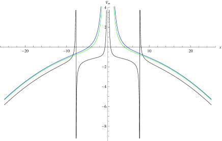
Figure 7: Effective partner potential $V_{\textbf{m}}(x)$ in (74) graphs. $\Phi=0.1,0.5,0.95$ corresponding to black, green, blue curves.

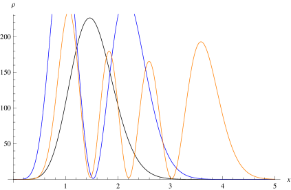
Figure 8: Probability density $\rho(r)=|u_{11}|^{2}+|u_{12}|^{2}$ graphs where $u_{12}$ is given by (56). $a=0.1,B=10,M=2,m=1,\alpha=0.2,\Phi=0.9,e=1$ and $n=0,1,3$ corresponding to black, blue, orange curves.

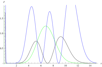
Figure 9: Probability density $\rho(r)=|u_{11}|^{2}+|u_{12}|^{2}$ graphs where $u_{12}$ is given by (75). $a=0.1,B=10,M=2,m=1,\textbf{m}=1,\alpha=0.2,\Phi=0.5,e=1$ and $n=0,1,2$ corresponding to green, black and blue curves correspondingly.

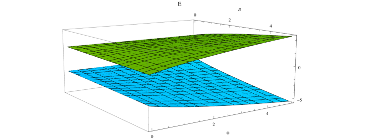
Figure 10: Energy levels given in (37) as a function of $B$ and $\Phi$. $a=0.2,B=10,M=2,m=1,\alpha=0.6,n=2,e=1$.

Finally, the probability density for the solutions in (75) and (38), and energy as a function of magnetic field strength and flux of the solenoid, are given in Figures $9$ and $10$, respectively.

4 Conclusions

This study demonstrates how the system of a spinning cosmic string spacetime, interacting with external fields via Aharonov-Bohm interaction, is adapted to rationally extended potential systems. Within these systems, the solutions of the partner Dirac Hamiltonian are found using SUSY QM and are expressed in terms of $X_{m}$ exceptional orthogonal Laguerre polynomials. The newly generated family of rationally expanded potentials has been identified as belonging to the class of nonlinear isotonic potentials. According to the analytical solutions, a sudden drop in magnetic field strength can lead to shifts and transitions in energy levels in Figure $1$ , which also agree with the results in [14]. It is also observed that when $\alpha<0.45$ and at smaller values of the magnetic field strength and flux, there are fewer positive energy levels compared to the energy of the antiparticles in Figure $5$. Moreover, the probability density graphs, which are obtained only for the smaller magnetic field strength and magnetic flux, are presented in Figures 8 and 9, in contrast to the probability density graph depicting greater magnetic field strength and magnetic flux in Figure 4. When we examine the change in energy levels with respect to $B$ and $\Phi$ in the Figure $10$, we find that the antiparticle’s eigenvalues are more numerous than those of the particle. By expressing wavefunction solutions in terms of exceptional $X_{m}$ Laguerre polynomials, we have both the advantage of deriving new exactly solvable potentials in (74) in terms of the string and magnetic field parameters, and it may also allow us to study systems with spectra that have ”gaps” or missing levels, which can be related to the study of supersymmetric quantum mechanics.

5 Data Availability Statement

Data sets generated during and/or analyzed during the current study are available from the corresponding author upon reasonable request. The data is housed within a secure repository to ensure compliance with ethical guidelines and privacy laws applicable to the study. Interested researchers may contact the corresponding author, providing a detailed explanation of their request and intended use of the data. Approval for data access will be subject to an assessment of the request’s alignment with the conditions under which the data was collected and any ethical or legal restrictions.

References

[1] T. W. B. Kibble, J. Phys. A: Math. Gen., Topology of cosmic domains and strings 9 1387–1398 1976.
[2] A. Vilenkin, Cosmic strings and domain walls, Phys. Rep. 121(5) 263-315 1985.
[3] I. Yu. Rybaka and L. Sousa, Emission of gravitational waves by superconducting cosmic strings, J. Cos. Astr. Phys. 11 024 2022.
[4] K. Kuijken, X. Siemens and T. Vachaspati, Monthly Notices of the Royal Astronomical Society, 384(1) 11 2008.
[5] K. Dimopoulos, Primordial magnetic fields from superconducting cosmic strings, Phys. Rev. D 57 4629-4641 1998.
[6]S. Nayak, S. Sau and S. Sanyal, Evolution of magnetic fields in cosmic string wakes, Astr. Phys. 146 102805 2023.
[7] T. Vachaspati and A. Vilenkin, Large-scale structure from wiggly cosmic strings, Phys. Rev. Lett. 67 1057 1991.
[8] Y. A. Sitenko, V. M. Gorkavenko and M. S. Tsarenkova, Magnetic flux in the vacuum of quantum bosonic
matter in the cosmic string background, Phys. Rev. D 106 105010 2022.
[9] B. Chakraborty, K. S. Gupta and S. Sen, Topology, cosmic strings and quantum dynamics - a
case study with graphene, Journal of Physics: Conference Series 442 012017 2013.
[10] M. M. Cunha and E. O. Silva, Self-Adjoint Extension Approach to Motion of Spin-1/2 Particle in the Presence of External Magnetic
Fields in the Spinning Cosmic String Spacetime, Universe, 6 203 2020.
[11] E. R. Bezerra de Mello, V. B. Bezerra, A. A. Saharian, and H. H. Harutyunyan, Vacuum currents induced by a magnetic flux around a cosmic string with finite core, Phys. Rev. D 91 064034 2015.
[12] E. R. Figueiredo Medeiros and E. R. Bezerra de Mello, Relativistic quantum dynamics of a charged particle in cosmic string spacetime in the presence of magnetic field and scalar potential ,The Eur. Phys. J. C, 72 2051 2012.
[13] M. Hosseinpour, H. Hassanabadi and M. de Montigny, The Dirac oscillator in a spinning cosmic string spacetime, Eur. Phys. J. C 79 311
2019.
[14] M. M. Cunha and E. O. Silva, Relativistic Quantum Motion of an Electron in Spinning Cosmic String Spacetime in the Presence of Unifor Magnetic Field and Aharonov-Bohm Potential, Adv. High En. Phys. 2021 6709140 2021.
[15] D S Citrin, The Aharonov–Bohm effect in quadratic Gauss quantum rings, Phys. Scr., 99 025914 2024.
[16] K. Bhattacharya, Demystifying the nonlocality problem in Aharonov–Bohm effect, Phys. Scr. 96 084011 2021.
[17] P. Auclair, K. Leyde and D. A. Steer, A window for cosmic strings, J. of Cosm. and Astr. Phys., 04 005 2023.
[18] W. Buchmüller, V. Domcke and K. Schmitz, Metastable cosmic strings, 11 020 2023.
[19] J. D. Garcia-Munoz and A. Raya, Supersymmetric quantum potentials analogs of classical electrostatic fields, Int. J of Geom. Meth. in Mod. Phys. https://doi.org/10.1142/S021988782450052.
[20] J. D. García-Munoz, D. J. Fernández and F. Vergara-Méndez, Supersymmetric quantum mechanics, multiphoton algebras and coherent states, Phys. Scr. 98 105243 2023.
[21] D. Gómez-Ullate, N. Kamran, R. Milson, An extension of Bochner’s problem: exceptional invariant subspaces. J. Approx. Theory 162(5), 987–1006 2010.
[22] M. A. Garcia-Ferrero, D. Gomez-Ullate and R. Milson, Exceptional Legendre Polynomials
and Confluent Darboux Transformations, Symmetry, Integrability and Geometry: Methods and Applications SIGMA 17 016 2017.
[23] S. Yadav, A. Khare, B. P. Mandal, Supersymmetry and shape invariance of exceptional orthogonal polynomials, 444 169064 2022.
[24] K. Bakke, Rotating effects on the Dirac oscillator in the cosmic string spacetime, Gen. Relativ. Gravit. 45 1847 2013.
[25] M. G. Alford and F. Wilczek, Aharonov-Bohm Interaction of Cosmic Strings with Matter, Phys. Rev. Lett. 62(10) 1989.
[26] M. M. Cunha, E. O. Silva, Relativistic quantum motion of an electron in spinning cosmic string spacetime in the presence of uniform magnetic field and Aharonov-Bohm potential, 2021 6709140 2021.
[27] K. S. Thorne, Closed timelike curves, 13th Int. Conf. on General Relativity and Gravitation 295
Cordoba, Argentina, 1992.
[28] M. Ringbauer, M. A. Broome, C. R. Myers, A. G. White and T. C. Ralph , Experimental simulation of closed timelike curves, Nature Communications 5 4145 2014.
[29] C. Quesne, Solvable Rational Potentials and Exceptional Orthogonal Polynomials in Supersymmetric Quantum Mechanics, Symmetry, Integrability and Geometry: Methods and Applications SIGMA 5 084 2009.
[30] F. M. Cooper, A. Khare and U. P. Sukhatme, Supersymmetry in Quantum Mechanics, World Scientific Publishing Company (July 3, 2001.
[31] R. L. Hall, N. Saad and Ö. Yeşiltaş, Generalized quantum isotonic nonlinear oscillator in d dimensions
, J. Phys. A: Math. Theor. 43 465304 2010.
[32] J. Sesma, The generalized quantum isotonic oscillator , J. Phys. A: Math. Theor. 43 185303 2010.
[33] ] D. Gomez-Ullate, N. Kamran, R. Milson, An extended class of orthogonal polynomials defined by a Sturm–Liouville problem, J. Math. Anal. Appl. 359 352 2009.
[34] D. Gomez-Ullate, N. Kamran and R. Milson, Exceptional orthogonal polynomials and the
Darboux transformation, J. Phys. A: Math. Theor. 43 434016 2010.
[35] R. K. Yadav, N. Kumar, A. Khare and B. P. Mandal, Rationally extended shape invariant potentials in arbitrary D-dimensions associated with exceptional polynomials, Acta Polytechnica 57(6) 477 2017.
[36] A. Bhattacharjie and E. C. G. Sudarshan, A Class of Solvable Potentials, Nuovo Cimento 25 864 1962.