Wall Shear Stress Generated by a Bernoulli Pad: Hot-Film Anemometry and Model Testing

Abstract

The wall shear stress generated by a Bernoulli pad over a workpiece is of interest for the particular application of non-contact biofouling mitigation from ship hulls. The shear stress distribution has been determined numerically in the literature; it is directly measured experimentally for the first time in this paper. A constant temperature anemometer is used with a hot-film sensor and water as the working fluid; the sensor is calibrated using fully developed channel flow. Experiments with a Bernoulli pad accurately capture the magnitude of the maximum shear stress and its location resulting from constriction of the flow and flow separation due to sudden change in direction from axial to radial. Several numerical models are tested against the experimental measurements.

1 Introduction

A Bernoulli pad is conventionally used to pick and place objects without contacting them [1, 2]. The pad is proximally located to the object or a workpiece, and axial flow through the center of the pad impinges on the workpiece and is deflected radially outward. The center of this impingement region is a stagnation point, where pressure is the highest. As the flow is deflected radially outward in the impingement region, the pressure decreases gradually but remains positive as it approaches the entrance to the pad’s gap. As such, this impingement region tends to repel the workpiece. The drastic increase in velocity due to the cross-section reduction at the entrance to the pad’s gap induces a pressure drop down to vacuum levels. As the flow expands radially outward inside the pad’s gap, the intensity of this vacuum reduces gradually. The vacuum present in the pad’s gap induces an attractive force on the workpiece. The balance between the repulsive force from the impingement region and the attractive force from the pad’s gap tends to fix the gap at a constant value. Any effort to take the pad from this equilibrium configuration is met with a resistive force. The effect of the gap on the nature of the normal force (attractive or repulsive) has been widely discussed in the literature [3]. The change in the nature of the force gives rise to both stable and unstable equilibrium configurations [4] but the presence of the stable equilibrium configuration allows the Bernoulli pad to be used for pick and place operations in industry [5, 6, 7].

In addition to normal forces, shear forces are generated by the flow field between the pad and the workpiece [8]. The shear forces generated by a Bernoulli pad have found the application of non-contact biofouling mitigation of ship hulls [9]. The abrupt change in the direction of flow introduces separation and recirculation near the neck of the pad [10]. The separation and constriction of the flow results in large magnitude shear stresses on the workpiece, which is essential for the application of bio-fouling mitigation. In our previous work [4], we have used computational fluid dynamics simulations to develop a better understanding of the flow physics, including the location and magnitude of the maximum shear stress. It was found that the magnitude of wall shear stress is maximum at the belly of the recirculation region. Resolving the region of flow separation is computationally expensive, which makes it challenging to predict the wall shear stress accurately. The numerical results need validation, and for the first time, in this paper a constant temperature hot-film anemometer is used with water as the working fluid to measure the wall shear stress.

Over the last few decades, various methods for wall shear stress measurements have been developed and reviewed in the literature [11, 12, 13]. The popular methods among researchers include the use of laser Doppler anemometer, floating element sensor, Preston or Stanton tubes, hot wire or hot-film, etc. Hot-film sensors have been used to detect flow separation and detection of transition from laminar to turbulent flow - see [14, 15, 16], for example. In the present work, we use a flush-mounted hot-film sensor for measurement of wall shear stress generated by a Bernoulli pad. The main principle behind this technique is to correlate heat transfer from the sensor with wall shear stress. To this end, the sensor needs to be calibrated under known wall shear conditions.

Experimental investigations with Bernoulli pads have been reported in the literature. Li and Kagawa [3], for example, conducted experiments to understand the various factors that affect the wall normal forces. A majority of the investigations in the literature have focused on wall-normal forces and used air as the working fluid. To the best of our knowledge, the only work with water as the working fluid was reported by Kamensky [17]; in this work, Particle Tracking Velocimetry (PTV) experiments were conducted to measure the velocity components of the flow field. PTV experiments do not provide reliable measurements close to the wall and cannot be used to accurately measure wall shear stress. Hence, the wall shear measurements presented in this work fill an important gap in the literature.

This paper is organized as follows. A brief review of the working principle of hot-film sensors is provided in Section 2. The calibration of the hot-film sensor is carried out using fully-developed channel flow; an analytical solution for wall shear in channel flow is presented in Section 2 and the procedure for calibration of the hot-film sensor is presented in Section 3. The experimental setup for wall shear measurements is described in Section 4. Section 5 provides experimental results and compares them with results obtained from numerical simulations. Concluding remarks are provided in Section 6.

2 Background

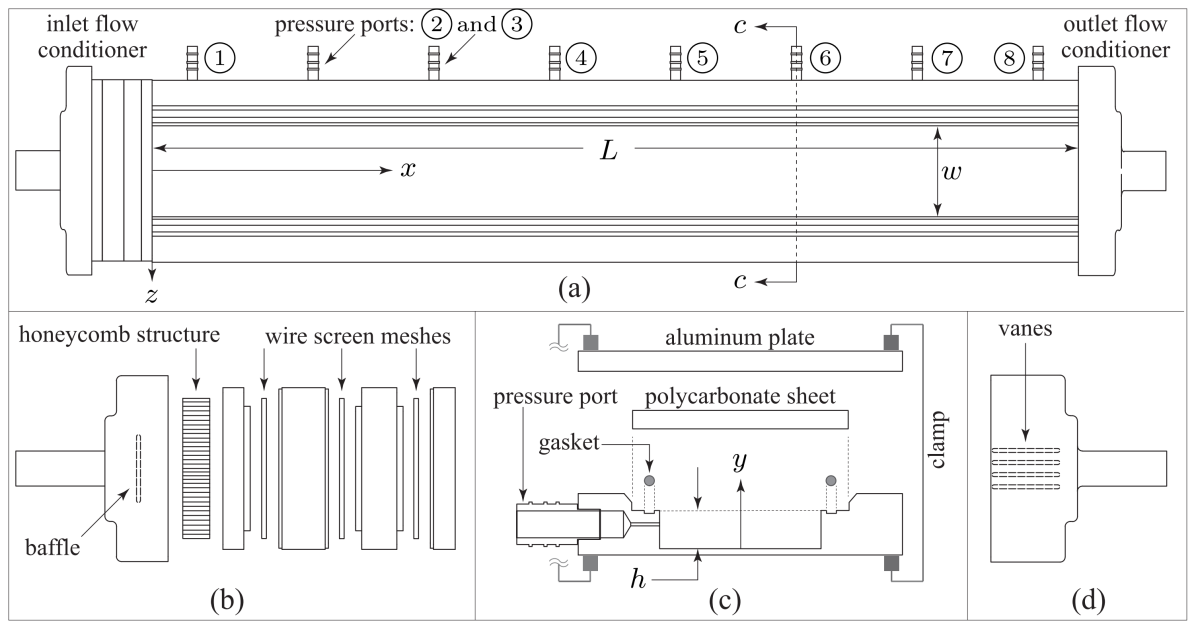
Figure 1: Channel setup used for calibration of the hot-film sensor; figures are not drawn to scale: (a) top-view of the channel showing the eight pressure ports, (b) exploded view of the inlet flow conditioner, (c) exploded view of section c-c of channel with gasket, polycarbonate sheet, aluminum plate, and clamps (d) outlet flow conditioner showing internal vanes.

2.1 Analytical solution for wall shear in channel flow

For two-dimensional steady-state fully developed channel flow - see Fig.1, the Navier-Stokes equation for the streamwise velocity becomes:

$$\mu\frac{d^{2}u}{dy^{2}}=\frac{dp}{dx}$$

where $p=p(x)$ is the pressure, $u=u(y)$ is the streamwise velocity, and $\mu$ denotes the dynamic viscosity. On integrating the above equation with respect to $y$ once, and substituting the symmetry condition $du/dy=0$ at $y=h/2$, we get:

$$\mu\frac{du}{dy}=\left(y-\frac{h}{2}\right)\frac{dp}{dx}$$ (1)

Note that $h$ is the channel’s height. This result does not assume any particular flow regime, laminar or turbulent. From the above result, the shear stress $\tau$ can be written as:

$$\tau\triangleq\mu\frac{du}{dy}=\left(y-\frac{h}{2}\right)\frac{dp}{dx}$$

At the wall, where $y=0$, the wall shear stress $\tau_{\rm w}$ is then given by:

$$\tau_{\rm w}=-\frac{h}{2}\frac{dp}{dx}$$ (2)

Therefore, the wall shear stress in channel flow can be determined by measuring the pressure gradient.

2.2 Working principle of hot-film anemometry

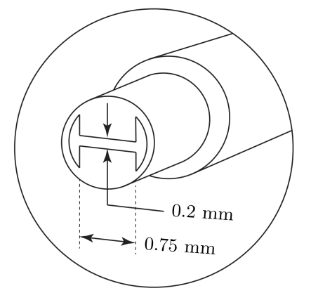
Figure 2: A schematic of the hot-film sensor 55R46 by Dantec Dynamics [18].

Hot-film anemometry is used to measure the velocity and turbulence properties of fluid flows. The hot-film sensor used in our experiments is shown in Fig.2. The H-shaped film at the tip of the sensor is a very thin electrical resistor. The main principle behind a hot-film anemometer is that the heat generated by electric current through the film is dissipated via thermal convection. The heat transfer rate from the film into the fluid varies with flow velocity according to King’s law [19]:

$$q_{\rm conv}=a+bu^{n},$$ (3)

and the heat generated by electric current is:

$$q_{\rm gen}=\frac{E^{2}_{\rm a}}{R_{\rm f}}$$ (4)

In (3) and (4), $a$, $b$, and $n$ are constants, $u$ is the characteristic velocity around the hot-film, $E_{\rm a}$ is the voltage applied across the film, and $R_{\rm f}$ is the film’s electrical resistance. To satisfy energy conservation, $q_{\rm conv}=q_{\rm gen}$. Hence, from equations (3) and (4):

$$E^{2}_{\rm a}=aR_{\rm f}+(bR_{\rm f})u^{n}$$ (5)

Since the hot-film anemometer will be calibrated with fully developed channel flow, (1) can be integrated with respect to $y$, using the non-slip boundary condition $u=0$ at $y=0$, to obtain an expression for $u$:

$$\mu u=(y^{2}-hy)\frac{1}{2}\frac{dp}{dx}$$

Very near the wall, for $y=\delta_{\rm nw}<<1$, the linear term dominates and the second order term becomes negligible. In turbulent boundary layers, $\delta_{\rm nw}$ is equal to or less than the thickness of the laminar sublayer. Under these conditions, the last result simplifies to:

$$\mu u\approx-\frac{dp}{dx}\frac{h}{2}\delta_{\rm nw}$$

From (2), we get:

$$u\approx\frac{\tau_{\rm w}}{\mu}\delta_{\rm nw}$$ (6)

Using (6), (5) can now be expressed in terms of the wall shear stress:

$$E^{2}_{\rm a}=aR_{\rm f}+bR_{\rm f}\left(\frac{\delta_{\rm nw}}{\mu}\right)^{n}\tau_{\rm w}^{n}$$ (7)

$R_{\rm f}$ is maintained constant when the sensor is operated with a Constant Temperature Anemometer (CTA). To this end, the hot-film is implemented within a Wheatstone bridge to constantly monitor and correct changes in its resistance due to cooling. The main compensation is achieved by changing the electric current through the film to maintain its temperature constant. Therefore, the coefficients of equation (7) can be absorbed into two calibration constants as follows:

$$E^{2}_{\rm a}=A+B\tau_{\rm w}^{n},$$ (8)

These constants are determined by correlating the voltage output of the sensor with known wall shear stress in fully-developed channel flow.

Though (8) was obtained without assuming any specific flow regime, heat transfer characteristics in laminar flows differ significantly from those of turbulent flows. In laminar flows, heat transfer is diffusion-dominated, whereas it is advection-dominated in turbulent flows because of transversal motions outside of the laminar sublayer. Therefore, the calibration constants of (8) should be different for laminar and turbulent flows.

3 Calibration of Hot-Film Sensor

3.1 Design of channel

The channel used for calibration of the hot-film sensor is motivated by prior work reported in the literature [20]. A schematic of the channel is shown in Fig.1(a) and a sectional view through a pressure port is shown in Fig.1(c). The channel was fabricated using Aluminum and its cross-section ($w=50$ mm, $h=5$ mm) was chosen to yield a Reynolds number of ${\rm Re}=10,\!000$ with the available pump. The length of the channel was chosen to be $L=1,\!200$ mm to ensure that the flow reaches a state of fully-developed flow under smooth-wall conditions, and remains so for a significant portion of the channel. The top of the channel is covered with a clear polycarbonate sheet and leakage is prevented through the use of a gasket along the length of the channel. An aluminum plate is placed over the polycarbonate sheet and clamps are used to apply uniform pressure on the gasket along the length of the channel to make it leak proof - see Fig.1(c) and Fig.3(a).

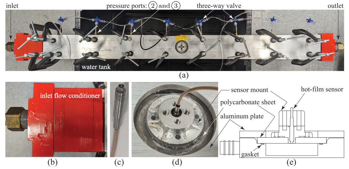
Figure 3: Assembled view of the channel setup in Fig.1: (a) top-view of the channel showing sensor mount (without sensor) and eight pressure ports (see Fig.1) connected via three-way valves, (b) inlet flow conditioner, (c) hot-film sensor, (d) magnified view of sensor mount with sensor, (e) sectional view of channel setup through the sensor mount and sensor.

A submersible utility pump was used to circulate water through the channel. The flow rate is controlled with a gate valve installed upstream of the channel’s inlet. The flow is conditioned at the inlet of the channel with a series of baffles, followed by a honeycomb, and then a series of three meshes of decreasing hole size - see Fig.1(b) and Fig.3(b). To reduce the developing length, the boundary layer is tripped with a coarse-grit sand paper strip at the inlet of the channel. The outlet of the channel is connected to a flow conditioner with four internal vanes to minimize end-effects - see Fig.1(d).

To measure pressure along the channel, eight pressure taps are placed on the side of the channel along its length. The ports are drilled with a size of $0.8$ mm. The ports are connected by a three-way valve - see Fig.3(a), to a DP15 differential pressure transducer (a product of Validyne Engineering [21]), not shown. The pressure differential between ports through relative to are recorded at steady state; the data is then used to compute the pressure at all the ports by assigning an arbitrary pressure to port - see Fig.4. The plot indicates that fully developed flow is achieved early and well ahead of port . The hot-film sensor can be mounted anywhere along the length of the channel in which the pressure drop exhibits a linear behavior, because that is the region where the flow is fully developed. We chose to mount the sensor, shown in Fig.3(c), between ports and on the polycarbonate sheet - see Fig.1(a), Fig.3(a) and Fig.3(d). A sectional view of the assembled channel setup through the sensor mount and sensor is shown in Fig.3(e).

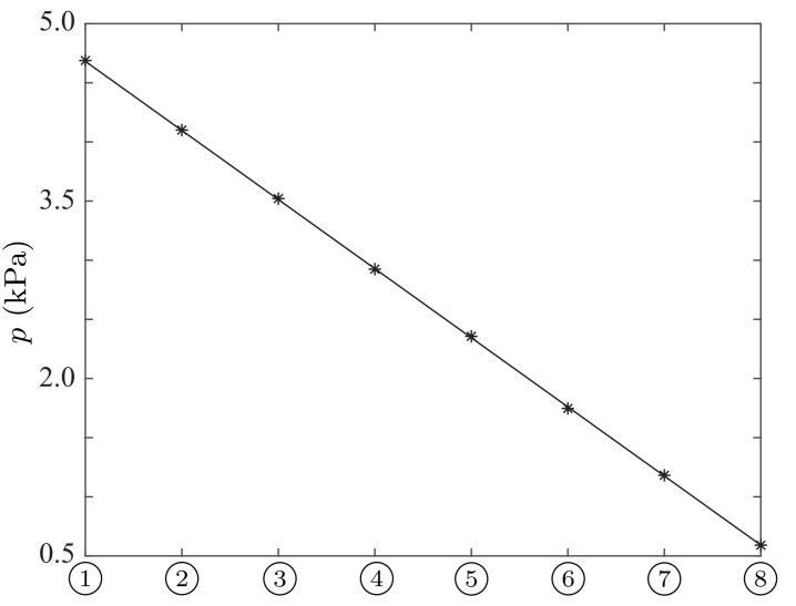
Figure 4: Pressure at the eight different ports of the channel (see Fig.1), computed based on pressure differential measurements relative to port and assignment of an arbitrary pressure to port . Note that the straight line fit was obtained by using the data from ports though .

3.2 Calibration procedure

The hot-film sensor 55R46, shown in Fig.2 and Fig.3(c), was calibrated using the constant temperature anemometer MiniCTA 54T42, also a product of Dantec Dynamics [18]. The sensor is used with water as the working fluid and therefore the jumpers inside the anemometer were adjusted according to the desired value of overheat and sensor resistance. The sensor is flush-mounted on top of the polycarbonate sheet between pressure ports and , where the flow is fully developed - see our discussion in Section 3.1.

The calibration of the sensor was performed using 21 different flow rates through the channel; a gate valve was installed between the prime mover and the inlet of the channel to control the flow rate. For each flow rate, the pressure transducer and hot-film sensor measurements (voltages) were recorded. The pressure measurement (voltage) provides the pressure drop between ports and ; transducer calibration data is used to express it in Pa and the wall shear stress $\tau_{\rm w}$ is then computed using Eq.(2). The variation of the square of the hot-film sensor voltage ($E_{\rm a}^{2}$) with the wall shear stress $\tau_{\rm w}$ is plotted in Fig.5 with the objective of computing the calibration coefficients in Eq.(8). It can be seen that the wall shear stress increases monotonically with increase in the mass flow rate. Also, the variation of $E_{\rm a}^{2}$ with $\tau_{\rm w}$ depicts three distinct behaviors corresponding to three distinct flow regimes: turbulent, critical and laminar. In the laminar and turbulent regimes, the data points show a concave downward trend with increase in wall shear stress; the trend is reversed and is concave upward in the critical regime.

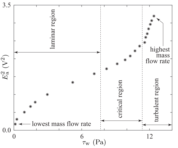
Figure 5: Calibration data showing the variation of $E_{\rm a}^{2}$ with $\tau_{\rm w}$

The data points corresponding to the laminar and turbulent regimes are used to find a linear fit between $E_{\rm a}^{2}$ and $\tau_{\rm w}^{n}$, where the value of the exponent $n$ should lie in the range $[0.1,0.5]$ [22]. A linear fit is found by choosing $n=0.4$ for the data in the laminar regime and $n=0.2$ for the data in the turbulent regime. The plots are provided in Fig.6 and the calibration coefficients in Eq.(8) are provided in Table 1; these coefficient were obtained with an $R^{2}$ value of $0.99$ and a confidence level of $95$%. The calibration coefficients in Table 1 will be used to measure the wall shear stress generated by a Bernoulli pad in Section 5.

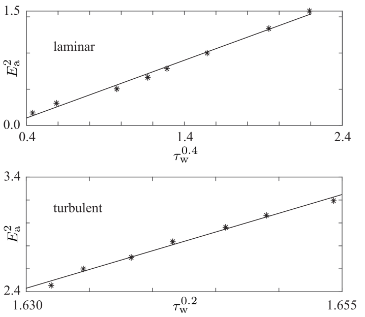
Figure 6: Linear calibration curves for laminar and turbulent regimes

Table 1: Calibration coefficients and exponent for laminar and turbulent flow regimes

Flow regime	$A$	$B$	$n$
Laminar	-0.216	0.798	$0.4$
Turbulent	-50.86	32.70	$0.2$

4 Bernoulli Pad Experimental Setup

An experimental setup was developed to measure the wall shear stress generated by a Bernoulli pad. An important component of the setup is the Bernoulli pad assembly, comprised of the stem, pad, and flow conditioning section - see Fig.7(a) and (b). The stem is a tube with an inside diameter of $d=25.4$ mm ($1.0$ in), an outside diameter of $31.75$ mm ($1.25$ in), and a length of $88.9$ mm ($3.5$ in). The pad is a circular, flat plate with a diameter of $D=203.2$ mm ($8.0$ in) and a thickness of $6.35$ mm ($0.25$ in). A $25.4$ mm ($1.0$ in) hole is located at the center of the pad along with a $31.75$ mm ($1.25$ in) counterbore to $75$% depth in the pad. The stem interfaces with the pad in the counterbore such that there are negligible steps for the fluid to encounter. Cast acrylic was selected as the material for both the stem and the pad; its rigidity is adequate for the current purpose and its surface roughness is very low. In particular, polished acrylic sheets typically exhibit a surface roughness within $0.14\,\mu{\rm m}<{\rm Ra}<0.23\,\mu{\rm m}$ [23], or equivalently, $0.62\,\mu{\rm m}<{\rm Rz}<0.89\,\mu{\rm m}$ [24]. Here, Ra is the arithmetic mean of the deviation from the roughness centerline, and Rz is the mean roughness depth.

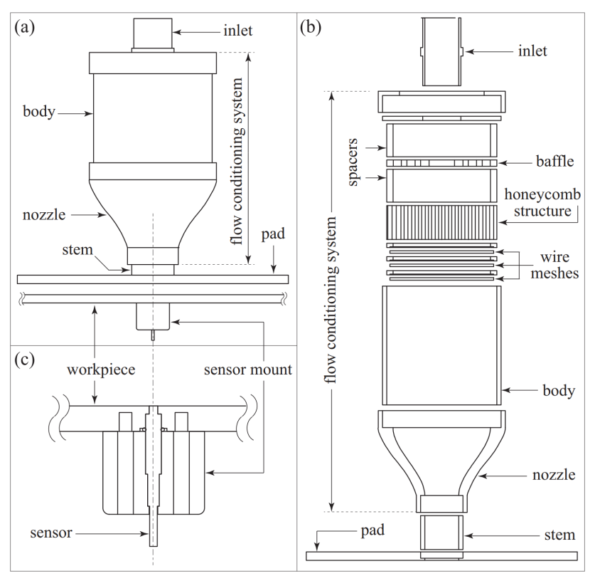
Figure 7: (a) Bernoulli pad assembly shown in its nominal configuration over the workpiece (b) exploded view of Bernoulli pad assembly (c) sectional view of flush-mounted sensor in workpiece.

The flow conditioning section is used to obtain a low-turbulence-intensity and top-hat velocity profile at the inlet of the stem. It is comprised of the following elements from upstream to downstream order: an inlet piece, a baffle that breaks down the incoming pipe flow, a honeycomb, three wire meshes of decreasing hole size, and a flow contraction - see Fig.7(b). A cubic equation was used to design the flow contraction profile [25]. The components of the flow conditioning section were mated with the stem in a similar fashion as the stem-pad interface to avoid disturbances in the flow. Except the inlet, baffle, honeycomb, and wire meshes, the materials of the components of the flow conditioning section were chosen as cast acrylic and polyurethane-coated 3D prints (fabricated with PLA - polylactic acid) for smooth surface finishes.

The primary components of the experimental setup are: workpiece, sensor mount, linear stage, Bernoulli pad assembly mount and frame. An assembled view of these components, which we will refer to as the Shear Test Station (STS), is shown in Fig.8. A rectangular, flat plate of 7075-T6 aluminum was selected as the workpiece because of its rigidity and electrical conductivity. It has dimensions of $406.4$ mm $\crossproduct$ $304.8$ mm $\crossproduct$ $6.35$ mm, and the surface of the workpiece was sanded and polished to reduce its surface roughness. This process typically results in roughness levels in the range of $0.1\,\,\mu{\rm m}<{\rm Ra}<0.4\,\,\mu{\rm m}$ or $0.5\,\,\mu{\rm m}<{\rm Rz}<1.4\,\,\mu{\rm m}$. Located at the center of the workpiece width and 254 mm down its length is a counterbored hole that allows the hot-film sensor to mate with the workpiece such that the sensing surface of the sensor is flush with the workpiece - see Fig.7(c). A grounding lead necessary for the hot-film sensor was permanently fastened to one of the plate’s vertical faces. Blind holes allow the sensor mount to be secured to the underside of the workpiece.

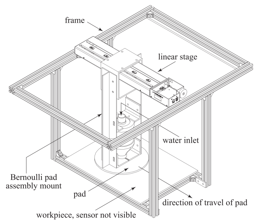
Figure 8: An assembled view of the Shear Test Station (STS), comprised of the Bernoulli pad assembly mount, workpiece and linear stage.

A LTS300 linear translation stage manufactured by THORLABS [26] was used to move the Bernoulli pad over the length of the workpiece such that the hot-film sensor can measure the wall shear stress along the radial direction. The LTS300 has an absolute accuracy of $50$ $\mu$m and a repeatability of $2$ $\mu$m. The Bernoulli pad assembly mount, shown in Fig.8, is a series of structural aluminum members that interface the Bernoulli pad assembly in Fig.7(a) to the linear stage. The joints of the Bernoulli pad assembly mount are comprised of slots and threaded fasteners that allow for setting a uniform gap between the pad and the workpiece. Structural aluminum extrusions form a frame that allows the workpiece to be positioned below the Bernoulli pad assembly mount and ensure that the pad and the workpiece remain parallel with travel of the linear stage. The fluid power assembly consists of a $250$ W submersible pump, rubber hoses, and a gate valve for flow rate control.

5 Wall Shear Stress Measurement

5.1 Procedure

The gap height between the pad and the workpiece was chosen to be $H=1.3$ mm for our experiments. Shims were placed in the gap to ensure that the gap height was uniform; they were removed after ensuring uniform desired gap height. The Shear Test Station (STS) was then placed into a water tank with dimensions of $2120$ mm $\crossproduct$ $749$ mm $\crossproduct$ $762$ mm - see Fig.9. The frame suspended the workpiece in the center of the tank footprint and $356$ mm from the bottom. The dimensions of the tank and the location of the workpiece were chosen to ensure that the radial outflow between the pad and workpiece was not affected by the water splashing from the tank walls. Shims were placed between the frame and tank to level the STS before it was secured to the tank with clamps. The fluid power assembly was connected, and the mass flow rate was set to $\dot{m}=0.046$ kg/s. The mass flow rate was chosen such that the maximum wall shear stress was within the range of the calibration setup. Sufficient water was added to the tank without submerging the workpiece and the water was allowed to adjust to the ambient temperature ($17.25^{\circ}$ C) before data collection began. The density and viscosity of water at this temperature are $\rho=998.87$ kg/m³ and $\mu=0.001073$ Pa s.

The pump was powered on, and the system was allowed to reach steady-state. The linear stage was used to move the Bernoulli pad from its nominal position, shown in Fig.7(a), in steps with an average size of $5$ mm, which is approximately twice the diameter of the hot-film sensor. The step size was reduced to $1.0$-$2.0$ mm close to the neck of the Bernoulli pad, where large variations in the shear stress are expected. The total distance of travel was approximately $\ell=83.0$ mm; this ensured that the sensor was never exposed to air. After each step, the sensor was powered on, and the hot-film sensor output was obtained using an oscilloscope. After recording the data, the sensor was powered off to avoid unnecessary heating.

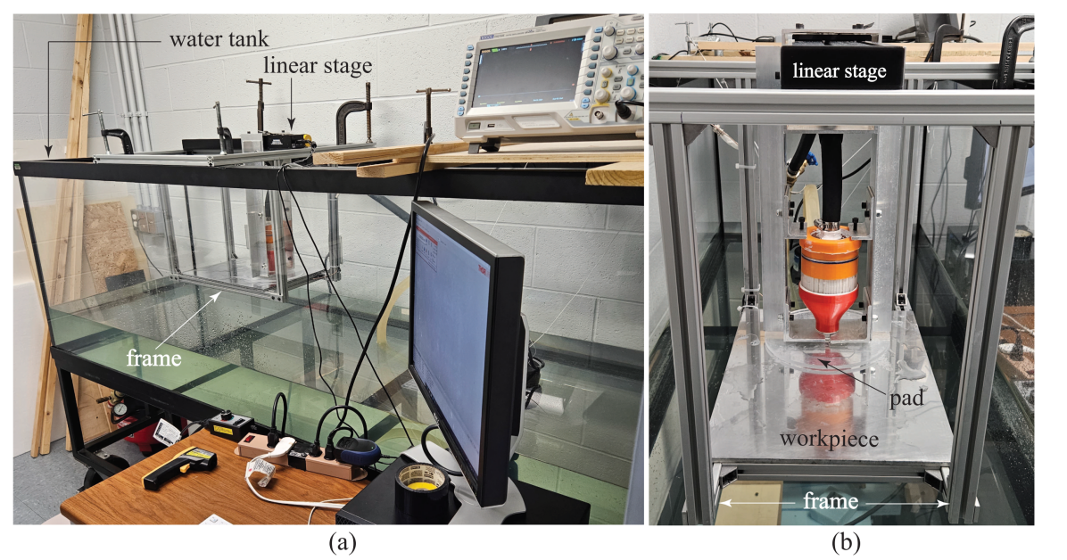
Figure 9: (a) A perspective view of the experimental setup (b) a side view showing the STS

The voltage outputs from the hot-film sensor were first corrected for temperature difference between calibration and wall shear stress measurement conditions. In particular, we used the following relation for temperature correction:

$$E_{\rm corr}=\left(\frac{T_{\rm f}-T_{0}}{T_{\rm f}-T_{\rm a}}\right)^{0.5}E_{\rm a}$$

where, $E_{\rm corr}$ is the corrected voltage, $T_{0}=25.49^{\circ}$C is the water temperature during calibration, $T_{\rm f}=40^{\circ}$C is the film temperature, and $T_{\rm a}=17.25^{\circ}$C is the water temperature during data acquisition. The corrected voltage values were used to obtain the wall shear stress values using Eq.(8) with the calibration coefficients provided in Table 1.

5.2 Comparison with numerical results

Numerical simulations were carried out using five different turbulence models, namely, Spalart-Allmaras, $\kappa$-$\varepsilon$, $\kappa$-$\omega$, Transition-SST, and RSM. These simulations were carried out for identical flow domain and boundary conditions in the experiments - see Fig.10. The domain is axially symmetric without variations in the azimuthal directions. Therefore, we used a two-dimensional axisymmetric model to reduce computational time. Assuming incompressible flow, we imposed a mass flow rate of $\dot{m}=0.046$ kg/s at the inlet, and exit pressure $p=p_{\text{atm}}$ at the pad’s outlet. Non-slip conditions were imposed on all solid walls.

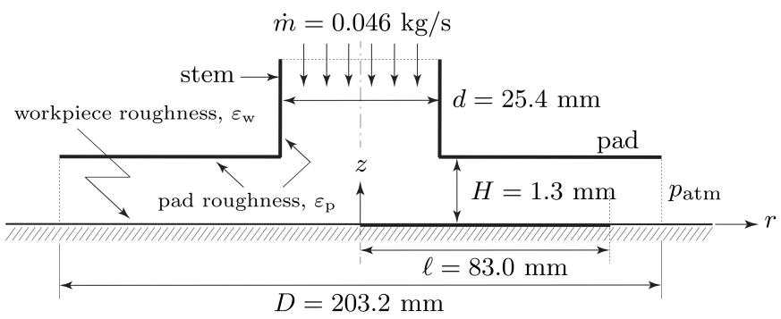
Figure 10: A schematic of the Bernoulli pad used in simulations.

Turbulence models implemented in commercial software require us to prescribe surface roughness level in solid walls. The choice of surface roughness level could be very relevant in fully rough flow, moderately important in transitionally rough flow, or completely unimportant in hydraulically smooth flow. The maximum wall shear stress measured in the current experiments was $\tau_{\text{w, max}}=10.19$ Pa. Hence, the maximum friction velocity was $u_{\tau_{\text{max}}}\triangleq\sqrt{\tau_{\text{w,max}}/\rho}=0.1$ m/s. Given that the thickness of the laminar sublayer in a turbulent boundary layer is $\delta^{+}_{l}\triangleq\rho\delta_{l}u_{\tau}/\mu=5$, our flow would be hydraulically smooth if its surface roughness’ representative height $\varepsilon_{\text{w}}<\delta_{l}=\delta_{l}^{+}\mu/(\rho u_{\tau})=49.5$ $\mu$m. As mentioned before, the roughness level in polished aluminum goes typically up to $\text{Rz}=1.4$ $\mu$m. Therefore, the flow through the pad’s gap is hydraulically smooth. For the simulations, any choice of roughness height for which $\varepsilon^{+}<5$ will have no roughness effects. With this in mind, the surface roughness of the pad and the workpiece were assumed to be $\varepsilon_{\text{p}}=\varepsilon_{\text{w}}=1$ $\mu$m to ensure hydraulically smooth conditions as in the experiments.

In our experiments, the hot-film sensor voltage is obtained for the measurement region of length $\ell=83.0$ mm shown in Fig.10. A comparison of these voltages with the voltage values in Fig.6 indicate that the flow is laminar for $r\in[0,12]\cup[14,83]$ and turbulent for $r\in[12,14]$, where the units are in mm. The change from laminar to turbulent flow close to the neck of the pad is expected due to the constriction of the flow and the formation of a recirculation region [10] due to flow separation upon change in the direction of flow from axial to radial around a sharp corner. To obtain the wall shear stress, we use the calibration coefficients in Table 1: the exponent and coefficient for laminar flow are used for $r\in[0,12]\cup[14,83]$ and those for turbulent flow are used for $r\in[12,14]$. The wall shear stress and radial distance are non-dimensionalized using the expressions in Anshul [4]:

$$\bar{\tau}_{\rm w}=\left(\frac{\pi\rho d^{3}}{4\dot{m}\mu}\right)\tau_{\rm w},\qquad\bar{r}=\left(\frac{2}{D}\right)r$$ (9)

The variation in the non-dimensional wall shear stress $\overline{\tau}_{\text{w}}$ with non-dimensional radial distance $\overline{r}$ is shown in Fig.11. No error bars are shown in these experimental results as the uncertainty associated with the measurements was found to be negligible (the extent of the error bars is less than the line thickness in the plot). For the purpose of model testing, the numerical simulation results from the five different turbulence models are also presented in Fig.11. All models coincide with each other for $0\leq\overline{r}\lesssim 0.14$ and $0.5\lesssim\overline{r}\leq 1.0$, but differ significantly from each other in the reattachment region.

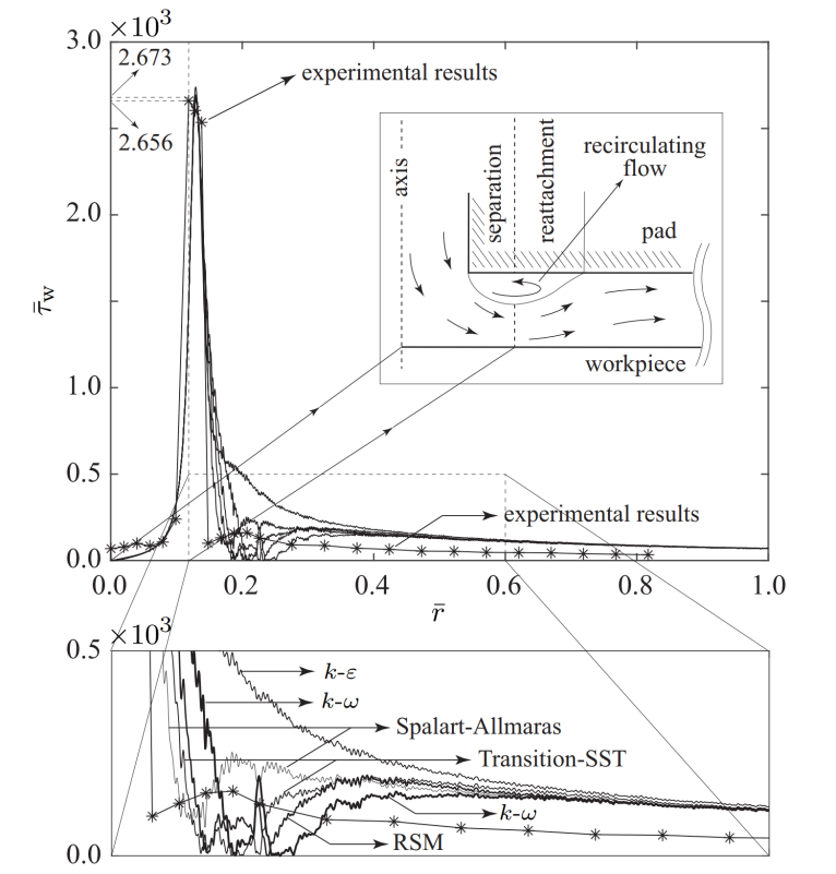
Figure 11: Variation of $\bar{\tau}_{\rm w}$ with $\bar{r}$: a comparison of simulation and experimental results. The experimental results, which were obtained at discrete values of $\bar{r}$, are shown using $*$ marks. The top figure shows the recirculation region and the flow around it [10] - see figure inset. A magnified view of the dotted portion of the top figure is shown in the bottom figure for comparison of the five different turbulence models with experimental results.

Overall, all models follow the qualitative behavior of the experimentally determined wall shear stress after the reattachment region. Nevertheless, all five turbulence models over-predict the wall shear stress values in this region. This is consistent with the experimental results from [4]. All numerical simulations predict both the magnitude and location of the maximum wall shear stress adequately, suggesting that all of them are able to capture the recirculation region reasonably well. The maximum non-dimensional wall shear stress $\tau_{\rm w,max}$ for all cases, including a power law estimation from [4], is shown in Table 2. The simulation results and the power-law prediction exhibit good agreement with the experimental results.

Table 2: Dimensionless maximum wall shear stress values obtained from experiment, numerical models, and power law [4]

Experiment	Spalart-Almaras	$\kappa$-$\varepsilon$	$\kappa$-$\omega$	Transition-SST	RSM	Power Law
$2656.1$	$2673.1$	$2741.4$	$2692.5$	$2676.3$	$2696.9$	$2548.6$

The experimental measurements show a secondary peak in wall shear stress right after the sharp drop from the maximum wall shear stress. This secondary peak is followed by a gradual decay in wall shear stress. This gradual decay in wall shear stress is easily explained by the $1/r$ proportional decay in radial velocity as the cross-sectional area of the pad gap increases with radius [27]. The secondary peak on the other hand is the result of reattachment phenomena. That is, the flow initially “squeezes” underneath the separation bubble forming a vena contracta and thinning the boundary layer. At the vena contracta, the flow is the fastest and the boundary layer is the thinnest, inducing the highest level of wall shear stress. The flow expands relatively rapidly toward the pad as it flows past the separation bubble. In this region, there is a localized change of direction as shown in the inset of Fig.11. Here, part of the linear momentum transfers from the radial direction to the wall-normal direction, with a resulting reduction in radial momentum. This results in the sharp drop of wall shear stress right after the vena contracta. But shortly after that, the momentum recovers its purely radial direction, and since the boundary layer is still very thin, the shear stress experiences a small boost. This is likely what causes the secondary peak in wall shear stress. Right after that, the boundary layer starts growing and the cross-section continues to grow with radius, causing the subsequent gradual reduction on wall shear stress.

Most of the models fail to capture the wall shear behavior in the reattachment region. The Spalart-Almaras model is the only scheme that exhibits the same qualitative behavior as the experimentally measured wall shear stress, though the secondary peak is located slightly further downstream than that in experiments. This result suggests that, in this model, the simulated streamwise extent of the separation bubble downstream of the vena contracta is larger than that in experiments. That the Spalart-Almaras performs better than the other models in the reattachment region is likely because this model performs well in wall-bounded flows at moderate to low Reynolds numbers under adverse pressure gradients.

All five turbulence models slightly over-predict the wall shear stress values for large values of $\overline{r}$. This is consistent with the comparison between simulations and Particle Tracking Velocimetry measurements in [4]. A better turbulence scheme, such as LES or DNS, may provide a better match for the entire domain of $\overline{r}$; however, this will require significantly higher computational effort and lies in the scope of future research. The most important aspect of a Bernoulli pad for grooming applications is its maximum wall shear stress; the details of the reattachment region are of relatively low importance. Henceforth, the results shown in Fig.11 suggest that our numerical solvers are appropriate to capture the most relevant features of flow through a Bernoulli pad, with the Spalart-Almaras scheme exhibiting a slight advantage over the others. It is then adequate to use this numerical model to optimize Bernoulli pad designs for improving grooming efficacy in non-contact biofouling mitigation.

6 Conclusion

The experimental work presented here uses a constant temperature anemometer with a hot-film sensor to quantify the wall shear stress generated by the action of Bernoulli pad over a proximally located workpiece. An experimental setup, consisting of a rectangular channel, is designed to calibrate the wall shear stress. The calibration of the sensor is carried out separately for laminar and turbulent regimes. These calibration relations are subsequently used to measure the wall shear stress generated by a Bernoulli pad. It should be mentioned that this experimental effort, which quantifies the wall shear stress generated by a Bernoulli pad with water as the working fluid, is the first of its kind.

Except for the reattachment region, numerical simulations exhibit good agreement with hot-film wall shear measurements. The position of the maximum wall shear stress is found to be very close to the neck of the Bernoulli pad, right below the belly of recirculation region. The predicted position and magnitude of the maximum wall shear stress are very close to the measured values. All tested computational models match each other beyond the reattachment region and capture the general trend of the wall shear stress, albeit slightly overestimating its value. The Spalart-Almaras model reasonably captures the wall shear-stress behavior in the reattachment region, while the rest of the models fail to do so.

References

- \bibcommenthead
- Paivanas and Hassan [1981] Paivanas, J.A., Hassan, J.K.: Attraction force characteristics engendered by bounded, radially diverging air flow. IBM Journal of Research and Development 25(3), 176–186 (1981)
- Misimi et al. [2016] Misimi, E., Oye, E., Lillienskiold, A., Mathiassen, J., Berg, O.A., Gjerstad, T.B., Buljo, J., Skotheim, O.: GRIBBOT – Robotic 3D vision-guided harvesting of chicken fillets. Computers and Electronics in Agriculture 121, 84–100 (2016)
- Li and Kagawa [2014] Li, X., Kagawa, T.: Theoretical and experimental study of factors affecting the suction force of a bernoulli gripper. Journal of Engineering Mechanics 140, 04014066 (2014)
- Tomar et al. [2022] Tomar, A.S., Kamensky, K.M., Mejia-Alvarez, R., Hellum, A.M., Mukherjee, R.: A scaling relationship between power and shear for Bernoulli pads at equilibrium. Flow 2, 29 (2022)
- McIlwraith and Christie [U.S. Patent No. 6601888, 2003] McIlwraith, L., Christie, A.: Contactless handling of objects (U.S. Patent No. 6601888, 2003)
- Wagner et al. [2008] Wagner, M., Chen, X., Nayyerloo, M., Wang, W., Chase, J.: A novel wall climbing robot based on Bernoulli effect, pp. 210–215 (2008)
- Brun and Melkote [2009] Brun, X., Melkote, S.: Analysis of stresses and breakage of crystalline silicon wafers during handling and transport. Solar Energy Materials and Solar Cells 93, 1238–1247 (2009)
- Kamensky et al. [2019] Kamensky, K., Hellum, A., Mukherjee, R.: Power scaling of radial outflow: Bernoulli pads in equilibrium. Journal of Fluids Engineering 141 (2019)
- Kamensky et al. [2020] Kamensky, K., Hellum, A., Mukherjee, R., Naik, A., Moisander, P.: Underwater shear-based grooming of marine biofouling using a non-contact bernoulli pad device. Biofouling 36, 951–964 (2020)
- Shi and Li [2016] Shi, K., Li, X.: Optimization of outer diameter of Bernoulli gripper. Experimental Thermal and Fluid Science 77, 284–294 (2016)
- Winter [1979] Winter, K.G.: An outline of the techniques available for the measurement of skin friction in turbulent boundary layers. Progress in Aerospace Sciences 18, 1–57 (1979)
- Fernholz et al. [1996] Fernholz, H.H., Janke, G., Schober, M., Wagner, P.M., Warnack, D.: New developments and applications of skin-friction measuring techniques. Measurement Science and Technology 7(10), 1396 (1996)
- Sheplak et al. [2006] Sheplak, M., Cattafesta, L., Nishida, T., Mcginley, C.: Mems shear stress sensors: Promise and progress. IUTAM Symposium on Flow Control and MEMS, 67–76 (2006)
- Bellhouse and Schultz [1966] Bellhouse, B.J., Schultz, D.L.: Determination of mean and dynamic skin friction, separation and transition in low-speed flow with a thin-film heated element. Journal of Fluid Mechanics 24(2), 379–400 (1966)
- Owen [1970] Owen, F.K.: Transition experiments on a flat plate at subsonic and supersonic speeds (1970)
- Jiang et al. [2000] Jiang, F., Lee, G.-B., Tai, Y.-C., Ho, C.-M.: A flexible micromachine-based shear-stress sensor array and its application to separation-point detection. Sensors and Actuators A: Physical 79(3), 194–203 (2000)
- Kamensky [Doctoral Dissertation, Michigan State University] Kamensky, K.M.: A new paradigm for generating surface-normal forces for hull-cleaning robots (Doctoral Dissertation, Michigan State University)
- [18] Dantec Dynamics: Flush-mounted hot-film probe. http://www.dantecdynamics.com/components/hot-wire-and-hot-film-probes/single-sensor-probes/film/, Last accessed on 2023-01-23
- King [1914] King, L.V.: Xii. on the convection of heat from small cylinders in a stream of fluid: Determination of the convection constants of small platinum wires with applications to hot-wire anemometry. Philosophical transactions of the royal society of London. series A, containing papers of a mathematical or physical character 214(509-522), 373–432 (1914)
- Sun et al. [2018] Sun, B., Wang, P., Luo, J., Deng, J., Guo, S., Ma, B.: A flexible hot-film sensor array for underwater shear stress and transition measurement. Sensors 18(10) (2018)
- [21] VALIDYNE Engineering: DP15 Variable Reluctance Pressure Sensor Capable of Range Changes. http://www.validyne.com/product/dp15_variable_reluctance_pressure_sensor_capable_of_range_changes/, Last accessed on 2023-01-26
- [22] Springer Handbook of Experimental Fluid Mechanics. Cameron Tropea, Alexander L. Yarin, John F. Foss (2007)
- S et al. [2011] S, S., Nair, C.K., Shetty, J.: Effect of Different Polishing Agents on Surface Finish and Hardness of Denture Base Acrylic Resins: A Comparative Study. International Journal of Prosthodontics and Restorative Dentistry 1(1), 7–11 (2011)
- Stähli [2013] Stähli, A.: The technique of lapping. Pieterlen/Biel (2013)
- Hussain and Ramjee [1976] Hussain, A.K.M.F., Ramjee, V.: Effects of the Axisymmetric Contraction Shape on Incompressible Turbulent Flow. Journal of Fluids Engineering 98(1), 58–68 (1976)
- [26] THORLABS: LTS300: 300 mm Linear Translation Stage with Integrated Controller, Stepper Motor. http://www.thorlabs.com/newgrouppage9.cfm?objectgroup_id=7652, Last accessed on 2023-01-26
- Guo et al. [2017] Guo, J., Shan, H., Xie, Z., Li, C., Xu, H., Zhang, J.: Exact solution to Navier-Stokes equation for developed radial flow between parallel disks. Journal of Engineering Mechanics 143(6) (2017)