Meta-stable states in the Ising model with Glauber-Kawasaki competing dynamics

Abstract

Meta-stable states are identified in the Ising model with competition between the Glauber and Kawasaki dynamics. The model of interaction between magnetic moments was implemented on a network where the degree distribution follows a power-law of the form, $P(k)\sim k^{-\alpha}$. The evolution towards the stationary state occurred through the competition between two dynamics, driving the system out of equilibrium. In this competition, with probability $q$, the system was simulated in contact with a heat bath at temperature $T$ by the Glauber dynamics, while with probability $1-q$, the system experienced an external energy influx governed by the Kawasaki dynamics. The phase diagrams of $T$ versus $q$ were obtained, which are dependent on the initial state of the system, and exhibit first- and second-order phase transitions. In all diagrams, for intermediate values of $T$, the phenomenon of self-organization between the ordered phases was observed. In the regions of second-order phase transitions, we have verified the universality class of the system through the critical exponents of the order parameter $\beta$, susceptibility $\gamma$, and correlation length $\nu$. Furthermore, in the regions of first-order phase transitions, we have demonstrated the instability due to transitions between the ordered phases through hysteresis-like curves of the order parameter, in addition to the existence of absorbing states. We also estimated the value of the tricritical points when the discontinuity in the order parameter in the phase transitions was no longer observed.

I Introduction

One of the main points of interest when dealing with non-equilibrium systems is the possibility of finding phase transitions with characteristics of reversible systems, even though in this non-equilibrium thermodynamic regime, we lack a unifying framework like a Gibbs equilibrium statistical mechanics [1]. We can handle non-equilibrium systems when the evolution process toward the steady state involves competition between two dynamics [2, 3, 4, 5]. This is because individually these dynamics satisfy detailed balance, but if both have a non-zero probability of acting on the system, the principle of microscopic reversibility is not always respected, and the system is forced out of equilibrium. Two dynamics that are commonly employed in competition are the Glauber dynamics with the single-spin flip process [6] and the Kawasaki dynamics with the two-spin exchange process [7].

Given its simplicity and usefulness in studying phase transitions, the Ising model is also widely employed in investigating non-equilibrium systems with competitive dynamics. In such cases, considering a ferromagnetic coupling between spins, with probability $q$, the system is in contact with a thermal reservoir at temperature $T$ and it relaxes to the steady state of lower energy through the Glauber dynamics. On the other hand, with probability $1-q$, the system is subject to an external energy influx, and evolves to the state of higher energy through the Kawasaki dynamics. In a regular square lattice [8], the Ising model subject to these competing dynamics self-organizes into the ordered phases, the ferromagnetic phase ($F$) and the antiferromagnetic phase ($AF$). In this self-organization, at low values of $q$, the $AF$ phase is found, corresponding to the higher energy state of the system. In contrast, when $q$ increases, a phase transition occurs to the paramagnetic phase ($P$). Further increasing $q$ leads to another transition to an ordered phase, the $F$ phase, corresponding to the lower energy state of the system. All these transition lines are of second-order.

Beyond regular networks, complex networks despite not having much evidence to describe crystals, are of great interest because they describe a range of structures found in society. Examples of these are the small-world networks [9, 10], which encompass the property discovered by Milgram [11], wherein any person in the world can have contact with another, requiring a remarkably smaller number of intermediaries compared to the size of the network. Another example of complex networks present in society are those that follow a power-law degree distribution, $p(k)\sim k^{-\alpha}$ [12]. In this case, $p(k)$ is the probability of any point in the network having $k$ other points connected to it, and $\alpha$ is the exponent that depends on the object of study. Networks of this kind are notable due to advancements in data processing techniques and equipment. It has been observed that networks such as the World Wide Web, the Internet, citation networks, networks of actors who have appeared in the same film, networks of protein interactions, among many others [13], despite having distinct formation origins, self-organize so that the degree distribution takes the form of a power law.

Due to the importance of complex networks, they have been implemented in physical models to investigate their influence on phase transitions [14, 15, 16, 17]. These models also include the non-equilibrium Ising model through competitive dynamics. The phenomenon of self-organization is observed with competing dynamics of one- and two-spin flips on small-world networks [18] and networks with power-law degree distribution [19]. This involves transitions from the $AF$ to $P$ phases and from the $P$ to $F$ phases, varying the competition parameter $q$. In both cases, only second-order phase transitions are found, and the universality class obtained through critical exponents, in both networks, with and without competitive dynamics, belongs to the mean-field regime [20, 21]. The results are also available regarding the Ising model on a 2D small-world network and with competition between the Glauber and Kawasaki dynamics [22]. In this case, the self-organization was also observed, but in the region of phase diagrams $(T\times q)$, where competition between the $F$ and $AF$ ordered phases are present, i.e., low values of $q$ and $T$, first-order phase transitions are found, in addition to second-order phase transitions for low values of $q$ with high values of $T$, and high values of $q$ with low values of $T$.

In the present work, we investigated the Ising model on a network with a power-law degree distribution and with competition between the Glauber and Kawasaki dynamics. In this configuration, each point of the network represents a spin variable that can take values of $\sigma\pm 1$, with a probability $p(k)\sim k^{-1}$ of interacting with $k$ other spins randomly distributed in the network. For the evolution towards the steady state, with probability $q$, the system is in contact with a thermal reservoir at temperature $T$ and it relaxes to the lowest energy state through Glauber dynamics. Meanwhile, with a probability $1-q$ , there is an external energy flux into the system, governed by Kawasaki dynamics, favoring the higher energy state. Thus, we aim to fill a gap in the study of non-equilibrium systems due to competitive dynamics in complex networks. We have found first-order phase transition lines in the Ising model on a complex network, as well as rich phase diagrams dependent on the initial state of the system, given the diffusive dynamic involved, with $AF$, $F$, and $P$ phases, and tricritical points separating first-order phase transitions from second-order ones.

This article is organized as follows: In Section II, we present the network, the dynamics involved in the system, and how they drive the evolution of the Ising system. In Section III, we provide details about the Monte Carlo method, the thermodynamic quantities of interest, and the scaling relations for each of them. The phase diagrams and a detailed description of both first- and second-order phase transitions present in these diagrams are discussed in Section IV. Finally, in Section V, we present the conclusions drawn from the study.

II Model

Here, we have utilized a network divided into two sublattices. The sites from one sublattice can only randomly connect to spins of the other sublattice, and the degree of the sites follows a power-law distribution of the form

$$p(k)=\frac{k^{-\alpha}}{\sum_{k=k_{0}}^{k_{m}}k^{-\alpha}}.$$ (1)

With $k_{0}=4$ being the minimum degree of the sites, $k_{m}=10$ the maximum degree present on the network, and a fixed value of $\alpha=1$, we impose limitations on the degrees of the network, thereby disrupting the scale-free network property typically found in real networks exhibiting growth and preferential connections [12]. This is done to ensure finite critical points and mean-field universality class, as our focus in this study is on the effects of reactive-diffusive competing dynamics on the well-defined network implemented in the Ising model. Further details on the network construction and the effect of the exponent $\alpha$ at the criticality of the system can be found in two previous works [19, 21].

In the Ising model, the interaction energy between the spins is defined by the Hamiltonian in the form

$$\mathcal{H}=-\sum_{\left\langle i,j\right\rangle}J_{ij}\sigma_{i}\sigma_{j}$$ (2)

where $\sigma_{i}=\pm 1$, the sum is over all pair of spins, and we use $J_{ij}=1$, meaning ferromagnetic interaction if sites $i$ and $j$ interact between the sublattices, and zero otherwise.

In the non-equilibrium system studied here, let us denote $p(\{\sigma\},t)$ as the probability of finding the system in the state $\{\sigma\}=\{\sigma_{1},...,\sigma_{i},...,\sigma_{j},...\sigma_{N}\}$ at time $t$. The equation governing the evolution of the probability of states over time is given by the master equation

$$\frac{d}{dt}p(\{\sigma\},t)=qG+(1-q)K,$$ (3)

where $qG$ represents the one-spin flip process, associated with the Glauber dynamics, which relaxes the spins in contact with a heat bath at temperature $T$, favoring the lowest energy state of the system, and it have probability $q$ to occur. On the other hand, $(1-q)K$ represents the two-spin exchange process, related with the Kawasaki dynamics, where the system is subjected to an external flux of energy into it, increasing the energy of the system, and it have probability $1-q$ to occur. $G$ and $K$ are described as follows:

$$\begin{array}[]{ccc}G=&\sum_{i,\{\sigma^{\prime}\}}\left[W(\sigma_{i}\to\sigma_{i}^{\prime})p(\{\sigma\},t)+\right.\\ &\left.-W(\sigma_{i}^{\prime}\to\sigma_{i})p(\{\sigma^{\prime}\},t)\right]&,\end{array}$$ (4)

$$\begin{array}[]{ccc}K=&\sum_{i,j,\{\sigma^{\prime}\}}\left[W(\sigma_{i}\sigma_{j}\to\sigma_{j}\sigma_{i})p(\{\sigma\},t)+\right.\\ &\left.-W(\sigma_{j}\sigma_{i}\to\sigma_{i}\sigma_{j})p(\{\sigma^{\prime}\},t)\right]&,\end{array}$$ (5)

where $\{\sigma^{\prime}\}$ is the new the spin configuration, $W(\sigma_{i}\to\sigma_{i}^{\prime})$ is the transition rate between the states on the one-spin flip process, and $W(\sigma_{i}\sigma_{j}\to\sigma_{j}\sigma_{i})$ the transition rate between the states in the two-spin exchange process.

III Monte Carlo simulations

In our Monte Carlo simulations, we have considered two possible initial states for the system: the ordered state, where all the spins are the same state, and the disordered state, where the spin states are randomly chosen. Starting from the initial state, a new spin configuration is generated following the Markov process: for a given temperature $T$, competition probability $q$, and network size $N=L\times L$, we randomly select a spin $\sigma_{i}$ in the network and generate a random number $r$, uniform distributed between zero and one. If $r\leq q$, we choose the one-spin flip process, in which the flipping probability is given by the Metropolis prescription:

$$W(\sigma_{i}\to\sigma_{i}^{\prime})=\left\{\begin{array}[]{cccc}e^{\left(-\Delta E_{i}/k_{B}T\right)}&\textrm{if}&\Delta E_{i}>0\\ 1&\textrm{if}&\Delta E_{i}\leq 0&,\end{array}\right.$$ (6)

where $\Delta E_{i}$ is the change in energy, based in Eq. (2), after flipping the spin $\sigma_{i}$, $k_{B}$ is the Boltzmann constant, and $T$ the temperature of the system. In summary, a new state is accepted if $\Delta E_{i}\leq 0$. However, if $\Delta E>0$ the acceptance is determined by the probability $\exp\left(-\Delta E_{i}/k_{B}T\right)$, and it is accepted only if a randomly chosen number $r_{1}$uniformly distributed between zero and one satisfies $r_{1}\leq\exp\left(-\Delta E_{i}/k_{B}T\right)$. If none of these conditions are satisfied, the state of the system remains unchanged. Now, if $r>q$ the two-spin exchange process is chosen, and in addition to the spin $\sigma_{i}$ we also randomly choose one of its neighbors $\sigma_{j}$, and the state of these two spins are exchanged according to transition rate

$$W(\sigma_{i}\sigma_{j}\to\sigma_{j}\sigma_{i})=\left\{\begin{array}[]{c}0\\ 1\end{array}\begin{array}[]{c}\textrm{if}\\ \textrm{if}\end{array}\begin{array}[]{cc}\Delta E_{ij}\leq 0\\ \Delta E_{ij}>0&,\end{array}\right.$$ (7)

where $\Delta E_{ij}$ is the change in the energy after exchange the state of the spins $\sigma_{i}$ and $\sigma_{j}$. In this process, the new state is accepted only if the change in the energy is greater than zero. Whereas this process aims to simulate the system under the influence of an external energy input, thus an increase in energy is expected.

Repeating the Markov process $n$ times, we have one Monte Carlo Step (MCS). We allowed the system to evolve for $n=10^{4}$ MCS to reach a stationary state, for all network sizes, $(32)^{2}\leq N\leq(256)^{2}$. To calculate the thermal averages of the quantities of interest, we conducted an additional $4\times 10^{4}$ MCS, and the averaging across samples was performed using $10$ independent samples for each configuration.

The measured thermodynamic quantities in our simulations are: magnetization per spin $\textrm{m}_{\textrm{N}}^{\textrm{F}}$, staggered magnetization per spin $\textrm{m}_{\textrm{N}}^{\textrm{AF}}$, magnetic susceptibility $\textrm{$\chi$}_{\textrm{N}}$ and reduced fourth-order Binder cumulant $\textrm{U}_{\textrm{N}}$:

$$\textrm{m}_{\textrm{N}}^{\textrm{F}}=\frac{1}{N}\left[\left\langle\sum_{i=1}^{N}\sigma_{i}\right\rangle\right],$$ (8)

$$\textrm{m}_{\textrm{N}}^{\textrm{AF}}=\frac{1}{N}\left[\left\langle\sum_{i=1}^{N}(-1)^{(l+c)}\sigma_{i}\right\rangle\right],$$ (9)

$$\textrm{{\hbox{\chi}}}_{\textrm{N}}=\frac{N}{k_{B}T}\left[\left\langle m^{2}\right\rangle-\left\langle m\right\rangle^{2}\right],$$ (10)

$$\textrm{U}_{\textrm{N}}=1-\frac{\left[\left\langle m^{4}\right\rangle\right]}{3\left[\left\langle m^{2}\right\rangle^{2}\right]},$$ (11)

where $\left[\ldots\right]$ representing the average over the samples, and $\left\langle\ldots\right\rangle$ the thermal average over the MCS in the stationary state. To facilitate the calculation of $\textrm{m}_{\textrm{N}}^{\textrm{AF}}$, the sites on the network are labeled as if we had a square lattice, $N=L^{2}$, in this way, $l$ and $c$ are the row and column of the site $i$, respectively. In Eqs. (10) and (11), $m$ can represent either $\textrm{m}_{\textrm{N}}^{\textrm{F}}$ or $\textrm{m}_{\textrm{N}}^{\textrm{AF}}$.

Near the stationary critical point $\Gamma_{c}$, the equations (8), (9), (10) and (11) obey the following finite-size scaling relations [23]:

$$\textrm{m}_{\textrm{N}}=N^{-\beta/\nu}m_{0}(N^{1/\nu}\epsilon),$$ (12)

$$\textrm{{\hbox{\chi}}}_{\textrm{N}}=N^{\gamma/\nu}\chi_{0}(N^{1/\nu}\epsilon),$$ (13)

$$\textrm{U}_{\textrm{N}}^{\prime}=N^{1/\nu}\frac{U_{0}^{\prime}(N^{1/\nu}\epsilon)}{\Gamma_{c}},$$ (14)

where $\epsilon=(\Gamma-\Gamma_{c})/\Gamma_{c}$ ($\Gamma$ can be $T$ or $q$), $\beta$, $\gamma$ and $\nu$ are the critical exponents related the magnetization, susceptibility and length correlation, respectively. The functions $m_{0}(N^{1/\nu}\epsilon)$, $\chi_{0}(N^{1/\nu}\epsilon)$ and $U_{0}(N^{1/\nu}\epsilon)$ are the scaling functions.

IV Results

This section is divided into four subsections. The subsections IV.1 and IV.2 are related to the phase diagrams obtained for the system with two different initial states. The subsections IV.3 and IV.4 concern to the different phase transitions types found in the phase diagrams, namely, second- and first-order phase transitions, respectively.

IV.1 Ordered initial state

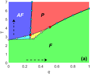
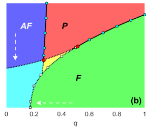
Figure 1: Phase diagrams $q$ as a function of $T$ for the ordered initial state of spins in the simulations. These diagrams present regions with different colors and denote the phases: $AF$ (purple), $F$ (green), $P$ (red), $AF$ or $F$ (cyan), and $F$ or $P$ (yellow). The cyan circles connected by solid lines indicate second-order phase transition points and the white squares connected by dashed lines indicate first-order phase transition points. The red points represent the tricritical points, and the black and white dashed arrows indicate the direction of sweeping of the parameters $T$ and $q$ in the simulations. The error bars are smaller than the symbol sizes.

In this subsection, the phase diagrams of the system were obtained with the ordered $F$ initial state in the simulations. In the diagram of Fig. 1(a), the phase transition points were found by varying the external parameters, $T$ or $q$, from the lowest to the highest value (see black arrows in the figure). At high values of $q$ and varying $T$, we have observed a second-order phase transition between the $F$ and $P$ phases. Thus, regardless of the initial state of the system and the starting point of the simulation, we consistently obtained the same critical point value. For temperatures $T\gtrsim 3.18$ and up to $T=6.235$, we have observed the self-organization phenomena in the system, where we start from the $AF$ phase, at low values of $q$, and pass to the disordered $P$ phase when reducing the external energy flow into the system. However, we found another ordered phase, the $F$ phase, when the prevailing dynamics involve the system being in contact with a heat bath, at high values of $q$. A characteristic of the critical points at high temperatures is that they indicate a second-order phase transition. On the other hand, at low values of $q$ and $T$, the first-order phase transitions are found. Regarding these first-order phase transitions, the cyan-colored region in the diagram indicates that we can have both the $F$ and $AF$ phases in this region, depending on the starting point of the simulations. If, we start the simulation with parameter values in the purple region, we find the $AF$ phase in the cyan region. Conversely, if we start the simulations with the parameter values in the cyan region, we only find the $F$ phase. The yellow region of the diagram indicates that we can have both the $P$ and $F$ phases in this region, depending on the initial parameter values of the simulations. If, we start the simulations with parameter values in the purple region, we find the $P$ phase in the yellow region. Nevertheless, if we initiated the simulations with parameter values in the cyan region, we find only the $F$ phase in the yellow region.

The existence of these phases can be explained by the dynamics implemented in the system. At low values of $q$, the Kawasaki dynamics prevail in the system, simulating an external energy flow into the system. In this dynamics, the order parameter is conserved, so if we have an initial state with all spins up, as is the case of the diagram in Fig. 1(a) at $q=0$, the only possible state is the $F$ state. However, if $q\neq 0$ the system is also influenced by the dynamics simulating the system in contact with a heat bath at temperature $T$, so at low temperatures, the $F$ phase is expected. Now, when the temperature increases, for low values of $q$, the Kawasaki dynamics that prevail in the system organize it into the $AF$ phase, the phase of higher energy of the system, as expected, because the dynamics governed by the Metropolis mechanism altered the spin states, so is possible to find a different state from $F$. Thus, for high values of $T$ and $q$, when the dynamics simulating a system in constant contact with a heat bath prevail in the system, the $P$ phase is found. Additionally, characterizing the first-order phase transitions, the cyan and yellow regions in the diagram indicate the instability of these states near the critical point and can be further identified in the results throughout this work.

In the diagram in Fig. 1(b) was also obtained with the ordered $F$ initial state in the simulations, but the points in this diagram were found by varying the values of the external parameters, $T$ or $q$, from the highest to lowest (see white arrows in the figure). In this case, the second-order phase transition points are the same as those in the diagram in Fig. 1(a), but the way we varied the external parameters allows us to observe new regions due to first-order phase transitions. Similar to the diagram in Fig. 1(a), the cyan region indicates both the $AF$ and $F$ phases, depending on the parameter values at the beginning of the simulation. If, we start the simulation with the parameter $q$ value in the purple region and decrease $T$, we always find the $AF$ phase, but if we start the simulation with the $T$ value in the cyan region, we only find the $F$ phase. The yellow region indicates both the $P$ and $F$ phases, depending on the parameter values at the beginning of the simulation. For instance, it we start the simulation with the parameter values in the red region, the yellow region represents the $P$ phase. However, if we start the simulation with external parameter values from the yellow region, we only find the $F$ phase. The cyan and yellow regions were delimited by the points from the diagram in Fig. 1(a). The first-order phase transition points present in the diagram in Fig. 1(b) were obtained by fixing $T$ and varying $q$, or fixing $q$ and varying $T$ starting from the purple or red regions.

The different regions of the diagram in Fig. 1(b), when compared to Fig. 1(a), result of the dynamics involved, as well as the values of the parameters that start the simulation and how they are changed. At low values of $q$ and high values of $T$, if $q\neq 0$, the influence of the heat bath on the system is sufficient to change randomly the spin states. Nonetheless, since the prevailing dynamics in the system force it towards the state of higher energy, we can still find the ordered state of the $AF$ phase. Maintaining low values of $q$ and starting from high values of $T$, when we decrease the temperature in the system, the influence of the dynamics simulating the heat bath in the system is insufficient to obtain an $F$ phase, and only the $AF$ phase is observed. However, at low values of $q$ and starting from $T$ values in the cyan-colored region, the temperature in the system is not high enough to have disordered spins, so the Glauber mechanism keeps the system ordered.

IV.2 Disordered initial state

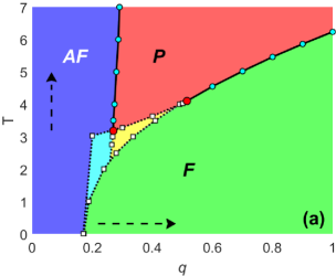
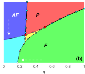
Figure 2: Phase diagrams $q$ as a function of $T$ for the random initial state of spins in the simulations. These diagrams present regions with different colors and denote the phases: $AF$ (purple), $F$ (green), $P$ (red), $AF$ or $F$ (cyan), and $F$ or $P$ (yellow). The cyan circles connected by solid lines indicate second-order phase transition points and the white squares connected by dashed lines indicate first-order phase transition points. The red points represent the tricritical points, and the black and white dashed arrows indicate the direction of sweeping of the parameters $T$ and $q$ in the simulations. The error bars are smaller than the symbol sizes.

Now, in the phase diagrams of Figs. 2(a) and (b), we have the steady states obtained for the system with the random spin initial state (disordered initial state) in the simulations. In Fig. 2(a), the variation of the external parameters, $T$ or $q$, occurs from the lowest to the highest value (see black arrows in the figure). When, we have a high external energy flow into the system, i.e., low values of $q$, only the ordered $AF$ state is found in the system. Yet, when we increase $q$, the first-order phase transitions from the $AF$ to $F$ phases are observed. In this diagram, the cyan-colored region indicates both the $AF$ and $F$ phases, depending on the value of the external parameter from which we start the simulation. If, the value of parameter $T$ starts as one of the values in the green region, the cyan region represents the $F$ phase. However, if the initial temperature of the system lies between the values of the cyan region, only the $AF$ phase is found in this region. The yellow region in the diagram of Fig. 2(a) can indicate both $F$ and $P$ phases. Starting the simulation with parameter values in the green region, the yellow region represents the $F$ phase. Now, if the parameter values are in the cyan or purple region, the phase found in the yellow region is the $P$ phase. Additionally, in this diagram the second-order phase transition points are the same as those found in the diagrams of Figs. 1(a) and (b).

The cyan and yellow regions in Fig. 2(a) can be interpreted as a meta-stable states due to the first-order phase transitions in this part of the diagram, where we have a greater influence of the diffusive dynamics, which conserves the order parameter (Kawasaki dynamics). In this figure, the initial state is one where the spin states are randomly distributed on the lattice sites. At low values of $q$, the high energy flow into the system ensures that we always obtain the state of higher energy, given the Hamiltonian of the Ising model. However, when the energy flow decreases, increasing $q$, the dynamics favoring the lower energy state prevail in the competition between dynamics, and we begin to find the $F$ state in the system for low values of $T$.

Finally, the diagram in Fig. 2(b), we also used the disordered initial state of the spins in the simulation, but now the sweeping of the external parameters occur from the highest to lowest values (see white arrows in the figure). In this diagram, we also have a region where can have both the $AF$ and $F$ phases. The cyan-colored region, when fixing $q$ and varying $T$, we only obtained the $AF$ phase. However, when fixing $T$ and varying $q$ and starting from values in the green region, only the $F$ phase is observed. The yellow region in this diagram also indicates both the $P$ and $F$ phases. If, the external parameters in the simulation are initialized with values from the yellow region, we find the $P$ phase in this region. On the other hand, if the parameter values at the beginning of the simulation are in the green region of the diagram, the yellow region refers to $F$ phase.

In Fig. 2(b), since the initial state of the spins is random and the parameters are swept from highest to lowest value, at low values of $q$, even though it is a dynamics that conserves the order parameter, such as the Kawasaki dynamics prevailing in the system, we always find the $AF$ phase. Increasing $q$, we find a first-order phase transition between the $AF$ and $F$ ordered phases. From these points, at low values of $T$, we only have the presence of the $F$ phase, since the system is simulated in contact with a heat bath at fixed $T$, where the one-spin-flip dynamics are prominent for high values of $q$. In this diagram, the meta-stable states of the first-order phase transitions in the cyan and yellow regions are also evident, along with the self-organization phenomenon mentioned in the description of Fig. 1(a), which can also be seen in all diagrams of Figs. 1 and 2.

IV.3 Second-order phase transitions

This subsection aims to present the critical behavior observed in the second-order phase transitions as can be seen in the diagrams of Fig. 1 and Fig. 2. The continuous variation of the order parameter during the transition from an ordered phase to the higher symmetry disordered phase can be identified by analyzing the crossing of the Binder cumulant curves at the phase transition point [24, 25]. In our system, the Ising model on the complex network with competing dynamics exhibits two regions in the phase diagram, of $T$ versus $q$, with second-order phase transitions.

The first region is observed at low values of $q$ and high of $T$, in the transition from the $AF$ to $P$ phase, as $q$ increases. In this part of the diagram, there is a high external energy flow into the system. Therefore, since the dynamics responsible for this energy flow favor the state of higher energy in the system, the$AF$ phase is expected to occur. This $AF$ phase is only observed at high values of $T$ in a second-order phase transition, because, due to the dynamics simulating the contact with the heat bath in the system, the only possible phase would be the disordered $P$ phase. Consequently, it prevents us from having a transition between two ordered phases, which is one of the main reasons why we find first-order phase transitions in the system.

Now, the second region where we found second-order phase transitions in the diagrams of Figs. 1 and 2 is the one with high values of $q$. In this case, the dominant dynamics in the system simulate the contact with the heat bath through the one-spin flip mechanism. This dynamics does not conserve the order parameter. Therefore, given favorable conditions, i.e., low temperatures, we will always find the state of lower energy, the $F$ phase, independently of the initial state of the system. This characteristic of the dynamics in the system prevents the existence of meta-stable states, and we can observe continuous phase transitions between the $F$ to $P$ phases.

The Binder cumulant curves for the two types of second-order phase transitions observed are present in Fig. 3. Fig. 3(a), we display the crossing of the curves indicating the transition point between $AF$ to $P$ phase as a function of $q$ and for a fixed value of $T=5.0$. At this same temperature, further increasing $q$, is observed transitions from the $P$ to $F$ phases, as indicated by the crossing of the Binder cumulant curves in Fig. 3(b). Transitioning from the ordered $AF$ phase to the disordered $P$ phase and from this disordered phase back to an ordered phase ($F$ phase), we can observe the phenomenon of self-organization in our non-equilibrium system.

Another property that we can obtain from the second-order phase transitions is the universality class of the system. This universality class can be identified through the critical exponents, which they were obtained here through the scale relations in Eqs. (12), (13) and (14). Using these scale relations, there are two main methods to obtain the exponents of the system.

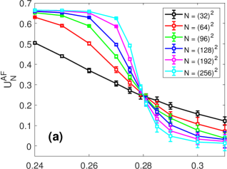
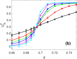
Figure 3: Binder cumulants $U_{N}^{AF}$ (a) and $U_{N}^{F}$ (b) as a function of the competition parameter $q$, and for a fixed value of $T=5.0$. The crossing point for different network sizes $N$ (see in the figure) indicate the second-order phase transition point in $q_{c}=0.28\pm 0.005$(a) and $q_{c}=0.694\pm 0.005$(b).

The first method can be seen in Fig. 4, where we have utilized the fact that scale relations are valid in the vicinity of the critical point. By collecting data of thermodynamic quantities at the phase transition for different lattice sizes $N$, the slope of the linear fit of these points on a graph with axes in logarithmic scale returns the ratios between the critical exponents. Using scale relation of Eq. (12), the points of the magnetization at $q_{c}$ as a function of $N$ yield the ratio $\beta/\nu$, as indicated by the linear fit of the black points in Fig. 4. Similarly, using the relation of Eq. (13), the susceptibility points show us the ratio $\gamma/\nu$, while with Eq. (14), utilizing data from the derivative of the Binder cumulant we obtain information about the exponent related to the correlation length, $1/\nu$. The linear fit for the ratios $\gamma/\nu$ and $1/\nu$ can be seen respectively in the red and green points in Fig. 4. Additionally, in this figure, the square points indicate the thermodynamic quantities at the transition between the $AF$ to $P$ phases, while circle points denote the quantities at the transition between the $P$ to $F$ phases. In these two transitions, the equivalent critical exponents are obtained, for $T=5.0$, at the $AF$ to $P$ phase transition we found $\left(\beta/\nu\right)_{AF}=0.24\pm 0.01$, $\left(\gamma/\nu\right)_{AF}=0.51\pm 0.02$, and $\left(1/\nu\right)_{AF}=0.51\pm 0.09$, while at the $P$ to $F$ phase transition we have obtained $\left(\beta/\nu\right)_{F}=0.26\pm 0.06$, $\left(\gamma/\nu\right)_{F}=0.50\pm 0.06$, and $\left(1/\nu\right)_{F}=0.49\pm 0.09$.

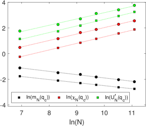
Figure 4: Linear fit of the thermodynamic quantities at the critical point as a function of the network size $N$, and for a fixed value of $T=5.0$. The square symbols represent the values of the $m_{N}^{AF}$, $\chi_{N}^{AF}$, and $U_{N}^{AF}$, already the circle symbols indicate the values of the $m_{N}^{F}$, $\chi_{N}^{F}$, and $U_{N}^{F}$. The results are well fitted by dashed straight lines. The error bars are smaller than the symbol sizes.

Another method that we can employ to find the critical exponents of the system is data collapse. This method aims to find the scaling function contained in the scaling relations by collapsing the data of thermodynamic quantities with different $N$. To achieve this, isolating the scaling function from the scaling relations, i.e., plotting $m_{N}N^{\beta/\nu}$ against $\epsilon N^{1/\nu}$ for magnetization curves, we adjusted the critical exponents until obtaining a single curve with the different $N$. When this occurs, the exponents used in this data collapse are the critical exponents of the system, since the scaling function is only obtained in the vicinity of the critical point and if the correct critical exponents of the system are used. In Fig. 5(a), we present the data collapse of the magnetization, $m_{N}^{AF}$ and $m_{N}^{F}$, while in Fig. 5(b), the data collapse of the susceptibility in the two transitions can be seen. These plots were made with logarithmic scale axes as this also allows us to identify the asymptotic behavior, far from $q_{c}$, of the scaling functions through the slope $\Theta$ presented in Figs. 5(a) and (b). Fixed at $T=5.0$, for the data collapse at the $P-AF$ transition, we used $\left(\beta/\nu\right)_{AF}=0.25$, $\left(\gamma/\nu\right)_{AF}=0.50$, $\left(1/\nu\right)_{AF}=0.50$, e $q_{c}=0.28\pm 0.005$, and at the $F-P$ transition, we have used the exponents $\left(\beta/\nu\right)_{F}=0.23$, $\left(\gamma/\nu\right)_{F}=0.52$, e $\left(1/\nu\right)_{F}=0.50$, along with the phase transition point $q_{c}=0.694\pm 0.005$.

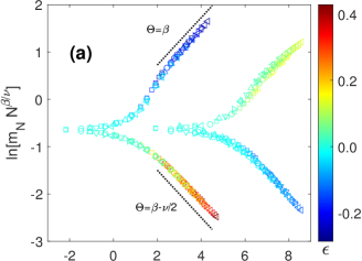
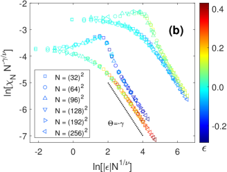
Figure 5: Data collapse of the magnetizations (a) and susceptibilities (b) for different network sizes $N$, as indicated in the figure, and for a fixed value of $T=5.0$. The curves of $m_{N}^{AF}$ and $\chi_{N}^{AF}$ can be seen in the right side of the figures, and for $m_{N}^{F}$ and $\chi_{N}^{F}$ the collapsed curves are in the left side of the figures. The data collapse validates our estimates for the critical parameters $\beta/\nu$ , $\gamma/\nu$, $1/\nu$, and$q_{c}$. The error bars are smaller than the symbol sizes.

In both methods used for calculating the critical exponents, we obtained equivalent results, and we can say that the system at the second-order phase transition belongs to the universality class of mean-field approximation, since $\beta=0.5$, $\gamma=1.0$, and $\nu=2.0$. These exponents are expected because we are dealing with the Ising model on a complex network where the second and fourth moments of the degree distribution are convergent. With this result, we have further evidence that the Ising model belongs to the same universality class both in thermodynamic equilibrium and out of it [21].

IV.4 First-order phase transitions

As mentioned in the description of the phase diagrams in Figs. 1 and 2, we found first-order transitions at low values of $q$. In this part of the diagrams, when we decrease $q$, we increase the external energy flow into the system. In this case, the Kawasaki dynamics tend to govern the system. As a dynamics that conserves the order parameter, it depends on initial conditions or complementary dynamics to reach specific steady states. If, we only have the Kawasaki dynamics acting on the system $(q=0$), as is predefined to favor the higher-energy state, and if the initial state of the system is $F$, then it will not be altered because the dynamics do not change the spin states. Additionally, if the initial state of the system is $P$, the system evolves to the $AF$ state, whereas this is the higher-energy state and the initial spin states do not need to be altered, only exchanged with each other. Now, if the system is in an initial $AF$ state, it remains unchanged. On the other hand, if there is a non-zero probability of the one-spin flip dynamics acting on the system ($q\neq 0$), as is strongly dependent on temperature and favors the lower-energy state of the system, at high values of $T$, the spin states are altered to be the disordered state $P$ as the steady state. Yet, if $q$ remains small, at these temperature values, the state of the system can be organized into the $AF$ phase because the Kawasaki dynamics still dominates the system. This phase is observed in all diagrams of Figs. 1 and 2 at second-order phase transitions.

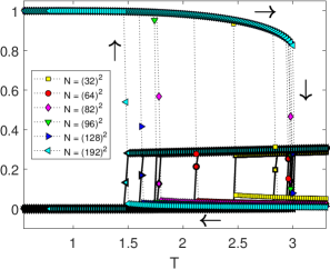
Figure 6: Behavior of the magnetization $m_{N}^{F}$ (dotted lines) and $m_{N}^{AF}$ (solid bold lines) as a function of $T$, and for different network sizes $N$, as indicated in the figure. Here, we used the fixed value of $q=0.2$. These hysteresis-like curves were obtained with the ordered $F$ initial state of the system, we start from the smallest to the largest value of $T$, and then in the opposite direction, as indicated by the arrows in the figure. The error bars are smaller than the symbol sizes.

For low values of $T$ and $q\neq 0$, we have two ordered state possibles for the system. This is because, from the Glauber dynamics, the steady state is the $F$ phase, while from the Kawasaki dynamics, we expect the $AF$ phase. In this case, the initial state of the system makes a total difference, because, starting from the initial $F$ state (see Fig. 1 (a)), even with the Kawasaki dynamics as the most dominant in the system, we do not find any other phase than $F$, which prevails for all values of $q$. On the other hand, if we have a disordered initial state (see Fig. 2(a) and (b)) or we start from an ordered state, but the system is disordered by the Glauber dynamics due to high temperatures (see Fig. 1(b)). When the Kawasaki dynamics is the most dominant, the system evolves into the ordered $AF$ state. However, at low temperatures, we have internal competition in the system between the dynamics, because, this is also the regime of the $F$ phase in the Glauber dynamics. So, if we decrease the external energy flow and the system is dominated by the heat bath, i.e., increasing $q$, an abrupt transition from the $AF$ to $F$ phases is observed. In these transitions between the ordered phases, we find the majority of the first-order transitions in the system. The transition between ordered phases can also be observed by changing the temperature of the system, i.e., at low values of $q$ and initial $F$ state, increasing $T$, the transition to $AF$ phase is observed.

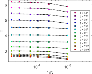
Figure 7: Linear adjustment of the temperature where we have the susceptibility peak, as a function of the inverse of the network size $N$, to estimate the critical point in the system. These adjustments were used to calculate the points in Fig. 1 (a), and here the x-axis is on a logarithmic scale just to better visualize the points.The error bars are smaller than the symbol sizes.

Due to the meta-stable states close to first-order phase transitions, one way to identify these transitions is by examining the dependence of the transition point on the system size. Another result of this instability is the possibility of obtaining hysteresis-like curves by changing the direction of parameter sweeping in first-order phase transitions. One of the most interesting points to observe these instabilities is $q=0.2$, because, it passes through all ordered phases and regions where both the ordered $F$ phase and the ordered $AF$ phase can exist. In Fig. 6, for the ordered $F$ initial state in the system, we present the plot of $m_{N}^{AF}$ and $m_{N}^{F}$, at $q=0.2$, as a function of $T$, varying from the lowest to the highest temperature, and then reversing, varying from the highest to the lowest temperature. Comparing these magnetizations with the phases obtained in the diagrams of Fig. 1, we can see that the approximate point where $m_{N}^{F}$ tends to zero is precisely on the transition line from the $F$ to $AF$ phase observed in the diagram of Fig. 1(a). As we decrease the temperature, we already have a nonzero value for $m_{N}^{AF}$, transitioning from the $AF$ to $F$ phase in the vicinity of the transition point in the diagram of Fig. 1(b).

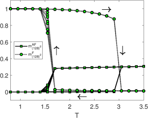
Figure 8: Behavior of the magnetizations $m_{N}^{F}$ and $m_{N}^{AF}$as a function of $T$ for network size $N=(128)^{2}$, and $q=0.2$. We performed $10$ cycles of variation of $T$, where the initial state of the system was with all spins in the same state. The error bars are smaller than the symbol sizes.

Owing to system size dependence, we can not use the crossing of the fourth-order Binder cumulant curves to obtain the first-order transition points of the system. However, we can use the linear behavior of the peaks of the magnetic susceptibility for different lattice sizes. In this case, we extrapolated the value of the critical point to an infinite-sized lattice, assuming that $T_{c}(\chi_{N}^{max})=N^{-1}\Delta+T_{c}(\chi_{N\to\infty}^{max})$, where $T_{c}(\chi_{N}^{max})$ is the pseudo-critical point for each network size and $T_{c}(\chi_{N\to\infty}^{max})$ is the extrapolation of the critical point for infinite network. Thus, we can fit $T_{c}(\chi_{N}^{max})$ as a function of $N^{-1}$ to obtain an estimate for $T_{c}(\chi_{N\to\infty}^{max})$ with the linear coefficient of this fit. Examples of these fits for different values of $q$ and for both first- and second-order phase transitions can be seen in Fig. 7, where we have placed the $N^{-1}$ axis on a logarithmic scale for better visualization of the points for the different network sizes after estimating the phase transition points.

As seen in Fig. 6, the hysteresis-like curves become even more unstable when dealing with regions in the phase diagram where two types of phases can coexist. Another way to observe this characteristic is by performing multiple loops of the external parameter, in this case $T$, for $q=0.2$, thus creating several hysteresis-like curves, as shown in Fig. 8. In this case, we have a single way when increasing $T$, but when we reverse the way, decreasing $T$, in this region where both $F$ and $AF$ phases can exist, we observe variations regarding the point where the transition between the ordered phases occurs.

When we decrease the external energy flux into the system, we reduce the main reason for the existence of first-order phase transitions, i.e., the coexistence between two ordered phases, as the prevailing dynamics in the system depends only on temperature and not on the initial state of the system or auxiliary dynamics. This reduction in the instability of the system until reaches the second-order phase transition when $q$ increases can be seen in Fig. 9: for the ferromagnetic magnetization curves in Fig. 9(a), Binder cumulant in Fig. 9(b), and magnetic susceptibility in Fig. 9(c). In this figure, the hysteresis-like curves were constructed somewhat differently from those in Fig. 6 and 8. The curves with square points represent results of the system with an ordered $F$ initial state, where all sites have the same spin value, while the points of the curves with circles represent a system with a random initial state (disordered sate). Additionally, the dashed curves indicate that $T$ was swept from higher to lower values, while the solid curves indicate that the temperature was swept from lower to higher values.

Another interesting point, that we can observe in Fig. 9 and in the phase diagrams of Figs. 1 and 2, is the existence of absorbing states which can be found at $q\lesssim 0.172$. In the case of $q=0.1$ in Fig. 9, we have an example of an absorbing state, i.e., starting from the ordered state and increasing the temperature, looking at $m_{N}^{F}$, we have a transition from $F$ to $P$ phase, but when we return in the opposite direction by decreasing the temperature, we have not reached the $F$ phase again. However, if we start from a disordered initial state, characteristic of $P$ phase, we never reach the $F$ phase. Another absorbing state, that can be identified at $q\lesssim 0.172$, is not shown here, but can be analyzed in Figs. 1 and 2. Looking at $m_{N}^{AF}$, if initially all spins in the system are in the same state, increasing the temperature transitions from $P$ to $AF$ phase is observed. Now, if we reverse the way by decreasing the temperature, we do not reach the $P$ phase again, only observing $AF$ phase. Starting from a disordered initial state and still considering $m_{N}^{AF}$, we always found phase $AF$ as the steady-state. This indicates that for $q\lesssim 0.172$, looking at $m_{N}^{F}$, once the $P$ phase is reached, we can not leave this phase, while looking at $m_{N}^{AF}$, once the $AF$ phase is reached, we can not leave this phase either. This characterizes the absorbing states and can be further verified in the phase diagrams of Figs. 1 and 2 for $q\lesssim 0.172$.

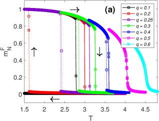
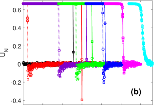
Figure 9: Behavior of the thermodynamic quantities of the system $m_{N}^{F}$ (a), $U_{N}$ (b), and $\chi_{N}$ (c) as a function of $T$. Here is presented curves for different values of $q$, as indicated in the figure, and for network size $N=(128)^{2}$. The solid curves denote the sweep of $T$ from the smallest to the largest value, while the dotted curves denote the sweep of $T$ from the largest to the smallest value. The curves with square points indicate that the system had an ordered $F$ initial state, while in the curves with circular points the initial state of the system is the disordered sate. The error bars are smaller than the symbol sizes.

In the phase diagrams of Figs. 1 and 2, we have found both first- and second-order phase transitions and the point where one type of transition starts and the other ends is where we can identify as the tricritical point. We do not have a very precise technique to define the tricritical point, but we can analyze some evidence that characterizes these types of phase transitions (first- and second-order) and estimate the value of this point. The most common characteristic between these two types of phase transitions is the continuity of the order parameter. For low values of $q$, we have a discontinuity of the order parameter in the first-order phase transition, while the continuous phase transition for high values of $q$ characterizes the second-order phase transitions (see Fig. 9). In addition to the discontinuity in first-order phase transitions, we also have evidence of coexistence between the ordered and the disordered phases, which can be verified with the distribution of the order parameter $\rho\left(m_{N}^{F}\right)$ in the vicinity of the critical point. Therefore, from Monte Carlo simulations, even if we apparently can not observe the discontinuity of the order parameter, when we analyze $\rho\left(m_{N}^{F}\right)$ in the vicinity of the critical point and observe the coexistence of phases and we can identify this as a first-order phase transition.

In Fig. 10(a), we display the $\rho\left(m_{N}^{F}\right)$ for some values of $q$ in the vicinity of the transition point. We can see $\rho\left(m_{N}^{F}\right)$ on the left side before $T_{c}$ and $\rho\left(m_{N}^{F}\right)$ on the right side after $T_{c}$. Before $T_{c}$, we can observe two maximum points representing the symmetric values of the order parameter, $\pm m_{N}^{F}$. After $T_{c}$, we have only one maximum point representing only the disordered phase, where $m_{N}^{F}=0$. For low values of $q$ in Fig. 10(a) and at the phase transition, we can observe three maximum points, indicating the coexistence of ordered and disordered phases, characteristic of a first-order phase transition. When we increase the values of $q$, we can not distinguish the peaks corresponding to the coexistence phases, indicating that we have a second-order phase transition. For instance, based on these distributions, we have estimated the tricritical point of the system given by $q_{t}=0.515\pm 0.01$ for $T=4.10$. Another tricritical point present in the phase diagrams of Figs. 1 and 2 is related to the transitions from the $AF$ to $F$ phase, and it was also estimated by this method, where we obtained $T_{t}=3.18\pm 0.02$ for $q=0.27$.

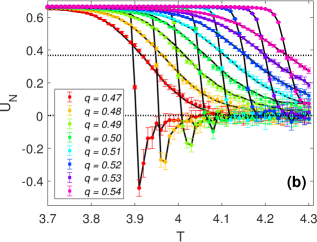
Figure 10: (a) The distribution $\rho\left(m_{N}^{F}\right)$ is presented for five values of $T$ around $T_{c}$ and values of $q$ near the tricritical point. Here, we used $N=(128)^{2}$. (b) Binder cumulant $U_{N}$ for $m_{N}^{F}$ with two network sizes $L=(32)^{2}$ (square symbols) and $L=(128)^{2}$ (circle symbols). The horizontal dashed lines are for $U_{N}=0$ and the crossing of the curves for $q=0.54$ at $U_{N}=0.367$.

We can also make an observation regarding the values of the Binder cumulant at the first-order phase transition. For this, with the same values of $q$ as in the distributions of Fig. 10(a), we present the curves for two different network sizes for the Binder cumulant in Fig. 10(b). With these curves, we can see that the Ising model on a complex network with competitive dynamics and in the first-order phase transitions, also presents negative values of the Binder cumulant. The dashed lines in Fig. 10(b) indicate references at $U_{N}=0$, and the point where the curves cross for $q=0.54$, $U_{N}=0.367$. This last reference line indicates that the crossing of the $U_{N}$ curves changes their values, and this remains even in the second-order phase transitions, and when $q=1.0$ the crossing is at $U_{N}=0.26$.

V Conclusions

We have employed Monte Carlo simulations to investigate the Ising model on a network with power-law degree distribution, subject to two competing dynamics. Considering the ferromagnetic coupling between spins, with probability $q$, the system is governed by Glauber dynamics, favoring the lowest energy state, while with probability $1-q$, the Kawasaki dynamics evolves the system towards the highest energy state. Given that Kawasaki dynamics conserves the order parameter, we built the phase diagrams $T$ versus $q$ with different initial states in the simulations. The topology of theses diagrams revealed regions with both first- and second-order phase transitions, leading to the discovery of tricritical points at coordinates ($q=0.27$,$T_{t}=3.18\pm 0.02$) and ($q_{t}=0.515\pm 0.01$,$T=4.1$). For $3.18\leq T\leq 6.235$ the self-organization phenomena is observed in the system. Here, at low $q$ values, the system exhibits the $AF$ phase, transitioning to the $P$ phase as $q$ increases, and further transitioning to an ordered phase, $F$ phase, for higher $q$. In regions of second-order phase transitions, we found that the universality class of the system is of mean-field approximation, with the critical exponents $\nu=2$, $\gamma=1$ and $\beta=0.5$. This universality class was expected due to dealing with networks where the second and fourth moments of the degree distribution are convergent [19, 21]. However, in these phase diagrams, we also observed first-order phase transitions, not previously observed in systems with dynamics that do not conserve the order parameter [18, 19], or systems with competing Glauber and Kawasaki dynamics, but in the regular networks[8]. This region, characterized by a discontinuity in the order parameter, arises due to the competition between $AF$ and $F$ ordered phases. This is because for low $q$ and $T$, the system tends to organize into a $AF$ phase due to the strong influence of Kawasaki dynamics, but for this, initially a disordered state of the system is necessary. On the other hand, simultaneously, as we are in the regime of low temperatures, even with the limited influence of Glauber dynamics, it is still possible to find the $F$ phase when starting with ordered initial state. Lastly, we have identified absorbing states in the system for below $q\lesssim 0.172$. Starting from the $F$ phase, at high $T$ the system transits to the $P$ phase when observing $m_{N}^{F}$, but when decreasing the temperature $T$, the $F$ phase is not recovered. Similarly, when observing $m_{N}^{AF}$, this absorbing state is the $AF$ phase, where now, analogously, we can not reach the $P$ phase at low $T$.

References

- [1] J. W. Gibbs. Elementary Principles in Statistic Mechanics. (Yale Universality Press, New Haven, 1902);
- [2] J. M. Gonzalez-Miranda, P. L. Garido, and J. Marro. Phys. Rev. Lett. 59, 1934 (1987);
- [3] T. Tom and M. J. de Oliveira. Phys. Rev. A, 40, 6643 (1989);
- [4] B. C. S. Grandi and W. Figueiredo, Phys. Rev. B, 50, 12595 (1994);
- [5] T. Tom , M. J. de Oliveira, and M. A. Santos. J. Phys. A: Math. Gen. 24, 3677 (1991);
- [6] R. J. Glauber, J. Math. Phys. 4, 294 (1963);
- [7] K. Kawasaki, Phys. Rev. 145, 224 (1966);
- [8] W. Figueredo and B. C. S. Grandi. Braz. J. Phys. 30, 58 (2000);
- [9] D. J. Watts and S. H. Strogatz, Nature (Lond.), 393, 440 (1998);
- [10] M. E. J. Newman and D. J. Watts, Phys. Rev. E 60, 7332 (1999);
- [11] S. Mingram, Psychol. Today, 1, 61 (1967);
- [12] A. -L. Barab si, R. Albert, Science, 286, 509 (1999);
- [13] R. Albert, A.-L. Barab si, Rev. Modern Phys. 74, 47 (2002);
- [14] A. L. M. Vilela, B. J. Zubillaga, C. Wang, M. Wang, R. Du, and H. E. Stanley. Sci. Rep. 10, 8255 (2020);
- [15] B. J. Zubillaga, A. L. M. Vilela, M. Wang, R. Du, G. Dong, and H. E. Stanley. Sci. Rep. 12, 282 (2022);
- [16] D. S. M. Alencar, T. F. A. Alves, R. S. Ferreira, F. W. S. Lima, G. A. Alves, and A. Macedo-Filho, Physica A, 626, 129102 (2023);
- [17] J. Wang, Wei Liu, F. Wang, Z. Li and K. Xiong, Eur. Phys. J. B, 22, 97 (2024);
- [18] R. A. Dumer and M. Godoy. Phys. Rev. E, 107, 044115 (2023);
- [19] R. A. Dumer and M. Godoy. Physica A, 626, 129111 (2023);
- [20] R. A. Dumer and M. Godoy. Eur. Phys. J. B 95, 159 (2022);
- [21] R. A. Dumer and M. Godoy. Physica A, 621, 128795 (2023);
- [22] W. Liu, Z. Yan, and G. Zhou, Open Phys. 17, 1 (2019);
- [23] H. Hong, M. Ha and H. Park. Phys. Rev. Lett., 98, 258701 (2007);
- [24] S.-H. Tsai and S. R. Salinas. Braz. J. Phys., 28, 1, (1998);
- [25] L. B ttcher and H. J. Herrmann. Computational Statistical Physics, 1rd ed. (Cambridge University Press, NewYork, EUA, 2021).