Inertial Torsion Noise in Matter-Wave Interferometers for Gravity Experiments

Abstract

Matter-wave interferometry is susceptible to non-inertial noise sources, which can induce dephasing and a resulting loss of interferometric visibility. Here, we focus on inertial torsion noise (ITN), which arises from the rotational motion of the experimental apparatus suspended by a thin wire and subject to random external torques. We provide analytical expressions for the ITN noise starting from Langevin equations describing the experimental box in a thermal environment which can then be used together with the transfer function to obtain the dephasing factor. We verify the theoretical modelling and the validity of the approximations using Monte Carlo simulations obtaining good agreement between theory and numerics. As an application we estimate the size of the effects for the next-generation of interferometery experiments with femtogram particles, which could be used as the building block for entanglement-based tests of the quantum nature of gravity. We find that the ambient gas is a weak source of ITN, posing mild restrictions on the ambient pressure and temperature, and conclude with a discussion about the general ITN constrains by assuming a Langevin equation parameterized by three phenomenological parameters.

I Introduction

Matter-wave interferometry has many salient applications for gravitational physics with devices spanning gravimeters [1], gradiometers [2, 3], accelerometers [4] and gyroscopes [5]. They can also be used for fundamental physics, such as testing the equivalence principle [6, 7, 8] and the quantum gravity induced entangled of masses (QGEM) to test the quantum nature of gravity in a lab [9, 10, 11, 12, 13] . Furthermore, some groups even consider building gravitational wave observatories based on matter-wave interferometry such as the matter-wave laser interferometer gravitation antenna (MIGA) [17, 18], the matter-wave atomic gradiometer interferometric sensor (MAGIS-100) [19, 20], as well as the mesoscopic interference for metric and curvature (MIMAC) scheme [21].

Future matter-wave interferometry aims to exploit the regime of large masses, large superposition sizes, and long coherence times, allowing the probe of exquisitely small experimental signals. For example, the (QGEM) experiment would ideally require a test mass of $\sim 10^{-15}$ kg, a superposition size of $\sim 100\,\rm\mu m$, and a coherence time of $\sim$1 s [9, 8, 22, 23, 24]. One of the most promising setups towards this kind of experiments is the adaptation of the Stern-Gerlach interferometer (SGI) to nanoparticles [25]. SGIs based on atom chips [26] have already achieved the superposition size and coherence time of 3.93 $\rm\mu m$ and 21.45 ms for the half-loop configuration [27], respectively, and $0.38\,\rm\mu m$ and 7 ms for the full-loop configuration [28], respectively. The next generation of SGIs is currently under theoretical and numerical investigation [29, 30, 31, 32, 33].

An essential challenge of matter-wave interferometry is to tame the numerous noise sources, which can cause random phase fluctuations, resulting in dephasing and the loss of interferometric visibility. Vibrations of the experiment apparatus can result in residual acceleration noise (RAN) [34, 35], external sources of gravity can induce gradient gradient noise (GGN) [35, 36, 18, 20], and charged or dipolar environmental particles can induce several electromagnetic channels of dephasing [37, 38], besides gravitational decoherence [39] of the QGEM.

This paper will study the dephasing caused by the residual rotational or inertial torsion noise (ITN) for an asymmetric nanoparticle matter-wave interferometer which is sensitive to gravity-gradients [21, 35, 36]. ITN arises naturally in any setup whenever the experimental apparatus is subject to random torques placing it in non-inertial rotational motion. As we will see, ITN can induce relative random phases in an interferometric experiment, resulting in a loss of interferometric contrast. Here, we will be primarily interested in understanding ITN, and we will focus on a simple single-stage suspension forming a torsion pendulum, i.e., matter-wave interferometry performed inside a hanging box. Analogous configurations of the experimental apparatus have been investigated previously in gravitational wave observatories like LIGO [40] and VIRGO [41]. More advanced setups could employ additional structures like the inverted pendulum [42] and the Roberts linkage [43].

In Sec. II, we first introduce the concept of ITN, illustrating it for matter-wave interferometry that can be modelled using qubits. In Sec. III, we generalize the analysis using linear response theory, providing the transfer function and its relation to the dephasing factor. In Sec. IV, we investigate ITN caused by ambient gas collisions on the experimental box starting from the classical Langevin equation. We will compute the power spectrum density (PSD) of the ITN using the convolution theorem and verify the validity of the approximations using Monte Carlo simulations. In Sec. V, we obtain the resulting constraints on the ambient pressure and temperature and general constraints on ITN by parametrizing a generic Langevin equation modelling the experimental box with three phenomenological parameters. In Sec. VII, we conclude with a summary of the obtained results. In Appendix A, we construct the ITN Lagrangian starting from Fermi normal coordinates and transforming to a rotating reference frame. In Appendix B, we provide for completeness also the complete derivation of the ITN PSD using complex analysis.

II Concept of Inertial Torsion Noise

Figure 1: (a) Experimental scheme and illustration of inertial torsion noise (ITN). The matter-wave particle (light and dark blue circles) is placed inside the experimental box (blue box), which is suspended by a thin wire (black vertical line). The box can rotate around the z-axis, while the interferometric protocol is performed along the horizontal x-axis. ITN generates random torques on the experimental box (blue rectangle), placing it in non-inertial rotational motion. The random non-inertial rotational motion induces random relative phases, which can lead to dephasing and the loss of interferometric contrast. (b) The structure of a Stern-Gerlach interferometer with spin-1 [25]. The left path keeps the same position, while the right path accelerates and decelerates at a constant rate resulting in a superposition size $\Delta x$. Such motion is achieved using a constant magnetic field gradient, i.e. $B(x)=B_{0}+\eta x$, where the gradient $\eta$ is positive during $0\sim t_{a}$ and $3t_{a}+t_{e}\sim 4t_{a}+t_{e}$, while it is negative during $t_{a}\sim 2t_{a}$ and $2t_{a}+t_{e}\sim 3t_{a}+t_{e}$. During the intermediate free flight of duration $t_{e}$, the magnetic field is uniform, and the right path does not accelerate. Such an asymmetrically shaped interferometer can be used to detect gravity-gradients [21, 35, 36]

Suppose the interferometer is set up in a suspended experiment apparatus, shown as Fig. 1(a). A natural reference frame is the comoving frame of the experimental apparatus. For instance, consider a Stern-Gerlach interferometer controlled by a static magnetic field $\mathbf{B}(x,y,z)$, which holds for the comoving frame of the experiment apparatus. If the SGI is studied under another reference frame which moves relative to the comoving reference, then the Lorentzian transformation of the magnetic field $\mathbf{B}(t)$ has to be taken into account, and even the induced electric field also needs to be studied. The comoving reference frame of the experiment apparatus is thus preferred as it simplifies the analysis.

However, the experimental apparatus itself can also be shaken by various environmental disturbances, such as vibrations of mechanical supports and jitter caused by collisions of air molecules. These vibrations of the experimental apparatus are applied to the interferometer as non-inertial forces, resulting in acceleration and rotation noises, affecting the interferometer’s final phase, i.e., residual acceleration noise (RAN) [35, 36] and inertial rotation noise (ITN) which we investigate in this paper. Such noises can induce dephasing, which can be mitigated only by carefully controlling the experimental setup and its environment.

In this paper, we will focus on the Stern-Gerlach interferometer with the configuration shown in Fig. 1(b), which can be achieved by a system with a spin-1 state and spin-0 state (embedded in an object) in a magnetic field with a constant gradient, see [21]. In particular, the system is prepared in a spin superposition of $\ket{S=0}$ and $\ket{S=1}$, say $\ket{\psi}=1/\sqrt{2}(\ket{S=0}+\ket{S=1})$, while the external magnetic field has a linear spatial distribution in the $x$-axis, i.e. $B(x)=B_{0}+\eta x$, where the magnetic gradient $\eta$ will flip several times to accelerate and decelerate the state $\ket{S=1}$.

Therefore, the acceleration of the $\ket{S=1}$ state is a constant $a_{m}=g\mu_{B}\eta$ during $0\sim t_{a}$ and $3t_{a}+t_{e}\sim 4t_{a}+t_{e}$, and $a_{m}=-g\mu_{B}\eta$ during $t_{a}\sim 2t_{a}$ and $2t_{a}+t_{e}\sim 3t_{a}+t_{e}$, where $g=2$ is the Lande factor and $\mu_{B}=9.27\times 10^{-24}$ J/T is the Bohr magneton.

In an ideal experiment (without any dephasing and decoherence), the final state of the system is

$$\ket{\psi}=\frac{1}{\sqrt{2}}\mathrm{e}^{\mathrm{i}\phi_{\rm global}}(\ket{S=0,L}+\mathrm{e}^{\mathrm{i}\phi_{\rm diff}}\ket{S=1,R}),$$ (1)

where $\phi_{\rm global}$ is the global phase of the quantum state and $\phi_{\rm diff}$ is the differential phase between two paths denoted as ”L” and ”R”. The global phase does not have observable effects, while the differential phase $\phi_{\rm diff}$ usually encodes the signal we want to extract. For example, $\phi_{\rm diff}$ is related to the gravitation acceleration $g$ for a gravimeter [44]. Another example is the QGEM experiment, which encodes information about the nature of gravity.

However, some classical noises like RAN and ITN always exist. They will contribute some random phase $\delta\phi$ on $\phi_{\rm diff}$. Although $\mathrm{e}^{\mathrm{i}\delta\phi}$ itself is a pure phase, the ensemble average of such a random phase can lead to a damping factor, known as a dephasing effect. For ease of convenience, $\delta\phi$ is supposed to follow a Gaussian distribution with a mean value of zero and a variance of $\Gamma\equiv\mathbb{E}[(\delta\phi)^{2}]$, then the expectation value of the phase can be computed as

$$\mathbb{E}[\mathrm{e}^{\mathrm{i}\delta\phi}]=\mathrm{e}^{-\mathbb{E}[(\delta\phi)^{2}]}\equiv\mathrm{e}^{-\Gamma},$$ (2)

where $\mathbb{E}[\cdot]$ is the ensemble average of random variables. Note that for a more general probability distribution of $\delta\phi$, one can also define a similar $\Gamma$ to describe the dephasing effect [45]. Such decay factor $\mathrm{e}^{-\Gamma}$ will cause the loss of visibility of the interferometer. In particular, consider the ensemble average of the density matrix $\hat{\rho}=\ket{\psi}\bra{\psi}$:

$$\begin{split}\mathbb{E}[\hat{\rho}]&=\frac{1}{2}\bigg{(}\ket{L}\bra{L}+\ket{R}\bra{R}\\ &+\mathbb{E}[\mathrm{e}^{\mathrm{i}\delta\phi}]\mathrm{e}^{2\mathrm{i}\phi_{\rm diff}}\ket{R}\bra{L}+\mathbb{E}[\mathrm{e}^{-\mathrm{i}\delta\phi}]\mathrm{e}^{-2\mathrm{i}\phi_{\rm diff}}\ket{L}\bra{R}\bigg{)},\end{split}$$ (3)

the off-diagonal terms decay exponentially with the damping given by the variance $\Gamma$. Consequently, the expectation value $\text{Tr}(\hat{W}\hat{\rho})$ of any witness operator $\hat{W}$ will also damp by the factor $\mathrm{e}^{-\Gamma}$.

Dephasing, together with all other types of decoherence, can be also characterized by computing the purity:

$$\text{Tr}(\mathbb{E}[\hat{\rho}]^{2})=\frac{1}{2}(1+\mathrm{e}^{-2\Gamma})\approx 1-\Gamma.$$ (4)

Note that the dephasing comes from the ensemble average of the density matrix. In particular, $\text{Tr}(\hat{\rho}^{2})$ without ensemble average still equals $1$. We will refer to $\Gamma$ as the dephasing factor in the following text. In the next section, we will analyze the dephasing factor $\Gamma$ caused by the ITN.

III Dephasing as Linear Response to Inertial Torsion Noise

As is derived in Appendix A, the Lagrangian of the inertial torsion noise is given by

$$L_{\rm ITN}=\frac{1}{2}m\dot{\Theta}^{2}x^{2},$$ (5)

where $m$ and $x$ are the interferometer’s mass and position, and $\Theta(t)$ is the torsion angle of the suspended apparatus, i.e., the angle between the apparatus reference frame and the inertial reference frame.

The angle $\Theta(t)$ is assumed to be a stochastic Gaussian process, satisfying the following two properties:

$$\mathbb{E}[\Theta(t)] =0$$ (6)

$$\mathbb{E}[\Theta(t_{1})\Theta(t_{2})] =\int S_{\Theta\Theta}(\omega)\mathrm{e}^{-\mathrm{i}\omega(t_{2}-t_{1})}\mathrm{d}\omega$$

where $S_{\Theta\Theta}(\omega)$ is the power spectrum density (PSD) of $\Theta(t)$ and the second identity is known as the Wiener-Khinchin theorem . The PSD of $\Theta$ can be measured in the experiment. In this paper, we will consider a specific sources of fluctuation of $\Theta$ (e.g., the collision by gas molecules, which will discussed in the next section).

Generally speaking, there are two dephasing channels in the leading order caused by this noise. First, the noise will contribute a phase along each path according to Feynman’s integral

$$\mathrm{e}^{\mathrm{i}\int L_{\rm ITN}[x^{(0)}(t)]/\hbar\mathrm{d}t}.$$ (7)

Secondly, the noise will also fluctuate the path of the two arms of the interferometer, so even the ideal phases along the paths will also be disturbed by a phase factor

$$\mathrm{e}^{i\int L_{0}[\delta x(t)]/\hbar\mathrm{d}t}.$$ (8)

The dephasing effect combining both channels is of higher order and can be neglected.

However, since the noise is assumed to be small, the fluctuations on the trajectories have to be small enough such that the final states of the two arms can meet each other. As a consequence, the second channel of dephasing has to be very small, while the first channel could be significant. Thus, we will focus on the phase fluctuation arising from Eq. (7):

$$\begin{split}\delta\phi&=\frac{1}{\hbar}\int L_{\rm ITN}[x_{R}(t)]-L_{\rm ITN}[x_{L}(t)]\mathrm{d}t\\ &=\frac{m}{2\hbar}\int\dot{\Theta}^{2}(t)\left(x_{R}^{2}(t)-x_{L}^{2}(t)\right)\mathrm{d}t,\end{split}$$ (9)

where $x_{R}(t)$ and $x_{L}(t)$ are the trajectories of the interferometer’s two arms. Assuming the expectation value of $\delta\phi$ vanishes, and the variance $\Gamma\equiv\mathbb{E}[(\delta\phi)^{2}]$ of the random phase can be regarded as the linear response of the interferometer to the torsion noise [35]:

$$\Gamma=\frac{m^{2}}{4\hbar^{2}}\int S_{\dot{\Theta}^{2}\dot{\Theta}^{2}}(\omega)F(\omega)\mathrm{d}\omega,$$ (10)

where $S_{\dot{\Theta}^{2}\dot{\Theta}^{2}}(\omega)$ is the PSD of the ITN. According to the Wiener-Khinchin theorem, the PSD is the Fourier transform of the autocorrelation function of the torsion noise

$$S_{\dot{\Theta}^{2}\dot{\Theta}^{2}}(\omega)=\int\mathrm{E}[\dot{\Theta}^{2}(t_{0})\dot{\Theta}^{2}(t_{0}+\tau)]\mathrm{e}^{\mathrm{i}\omega\tau}\mathrm{d}\tau.$$ (11)

Note that $S_{\dot{\Theta}^{2}\dot{\Theta}^{2}}(\omega)$ has a unit of $\rm Hz^{4}/Hz$, where $\rm Hz^{4}$ comes from the square of $\dot{\Theta}^{2}$ and the denominator $\rm Hz$ describes the density of frequency space. The $F(\omega)$ in Eq. (10) has the unit $\rm m^{4}s^{2}$, and is given by

$$F(\omega)=\left|\int\left(x_{R}^{2}(t)-x_{L}^{2}(t)\right)\mathrm{e}^{\mathrm{i}\omega t}\mathrm{d}t\right|^{2}.$$ (12)

Eq. (10) describes the input-output relation of the interferometer and only depends on the trajectories of the two arms, so it can be called the transfer function of the interferometer[36]. For the interferometer in Fig.1(b), the left arm is static $x_{L}(t)\equiv 0$, and the right arm $x_{R}(t)$ is described by a piecewise function consisting of several quadratic functions of $t$ because the acceleration is $\pm a_{m}$ for the different time range. Then the transfer function can be computed as

$$\begin{split}F(\omega)&=16\frac{a_{m}^{4}}{\omega^{10}}\bigg{[}6\omega t_{a}\cos\left(\omega(t_{a}+\frac{t_{e}}{2})\right)+\left(\omega^{2}t_{a}^{2}+3\right)\sin\frac{\omega t_{e}}{2}\\ &-3\sin\left(\omega(2t_{a}+\frac{t_{e}}{2})\right)-\omega^{2}t_{a}^{2}\sin\left(\omega(t_{a}+\frac{t_{e}}{2})\right)\bigg{]}^{2}.\end{split}$$ (13)

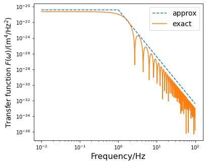
Figure 2: Transfer function of the interferometer illustrated in Fig.1(b) as a function of the frequency $f=\omega/(2\pi)$. The time parameters are $t_{a}=0.25$ s and $t_{e}=0$ s. The magnetic field gradient $\eta$ is chosen as $10^{4}$ T/m and the mass of the interferometer is chosen as $10^{-15}$ kg. The resulting acceleration $a_{m}=1.8\times 10^{-4}\,\rm m/s^{2}$ produces the maximum superposition size $\Delta x=a_{m}t_{a}^{2}=11.2\,\rm\mu m$. As is shown, the transfer function tends to a constant $C\sim(\Delta x)^{4}T^{2}\sim 10^{-20}\,\rm m^{4}s^{2}$ at low frequencies, and decreases as $\omega^{-6}$ at high frequencies. The approximate transfer function from Eq. (14) (dashed blue line) captures the behaviour of the transfer function from Eq. (13) (orange line).

Fig.2 shows the transfer function with the parameters chosen as $t_{a}=0.25$ s, $t_{e}=0$ s and $a_{m}=1.8\times 10^{-4}\,\rm m/s^{2}$, where $a_{m}=g\mu_{B}\eta/m_{0}$ with the magnetic field gradient $\eta=10^{4}$ T/m and the mass of the interferometer $m_{0}=10^{-15}$ kg.

As is shown in Fig.2, $F(\omega)$ tends to a constant $C\sim(\Delta x)^{4}T^{2}\sim 10^{-20}\,\rm m^{4}s^{2}$ in low frequency limit , where $\Delta x=a_{m}t_{a}^{2}=11.2\,\rm\mu m$ and $T=4t_{a}+t_{e}$ are the superposition size and the total experiment time. On the other hands, $F(\omega)$ decrease as $\omega^{-6}$ in high frequency . Combining the low-frequency and high frequency behaviours of $F(\omega)$, one can use the Heaviside step function $\theta(\cdot)$ to approximately describe $F(\omega)$ as

$$F(\omega)\approx(\Delta x)^{4}T^{2}\left(\theta\left(\frac{2\pi}{T}-\omega\right)+\left(\frac{2\pi}{T\omega}\right)^{6}\theta\left(\omega-\frac{2\pi}{T}\right)\right).$$ (14)

IV Power Spectrum Density of Inertial Torsion Noise

In this section, we will analyze the inertial torsion noise caused by the thermal motion of gas molecules surrounding the experimental box.

According to the convolution theorem, the PSD of ITN is the self-convolution of the PSD of the random motion of the suspended apparatus

$$S_{\dot{\Theta}^{2}\dot{\Theta}^{2}}(\omega)=S_{\dot{\Theta}\dot{\Theta}}(\omega)\ast S_{\dot{\Theta}\dot{\Theta}}(\omega),$$ (15)

where $S_{\dot{\Theta}\dot{\Theta}}(\omega)$ is the PSD of $\dot{\Theta}$. In frequency space, there is a correspondence that $\dot{\Theta}\sim\mathrm{i}\omega\Theta$, so the PSD of $\dot{\Theta}(t)$ is

$$S_{\dot{\Theta}\dot{\Theta}}(\omega)=\omega^{2}S_{\Theta\Theta}(\omega).$$ (16)

As is shown in Fig. 1(a), the rotational motion of the experimental box can be modelled as a torsion pendulum. The intrinsic torsion frequency is given by[47]

$$\Omega_{\rm rot}=\sqrt{\frac{\kappa}{I}}=\sqrt{\frac{\pi\mathbb{G}d^{4}}{32lI}},$$ (17)

where $I$ is the moment of inertia of the experiment box and $\kappa=\sqrt{\pi\mathbb{G}d^{4}/32l}$ is the torsion constant. $\mathbb{G}$ is the shear modulus of the material of the suspension wire, $d$ and $l$ are the diameter and the length of the wire. The size and the mass of the experiment box can be built up as $10^{-1}\sim 10^{0}$ m and $10^{1}\sim 10^{2}$ kg, so the moment of inertia $I$ can be estimated as $10^{0}\sim 10^{2}\,\rm kg\cdot m^{2}$. The parameters of the suspension wire are around $d=10^{-3}\sim 10^{-2}$ m, $l=10^{0}\sim 10^{1}$ m and $\mathbb{G}\sim 10^{10}$ Pa, then the intrinsic frequency $\Omega_{\rm rot}$ of the torsion pendulum is around $10^{-2}\sim 10^{1}$ Hz.

For example, if the experiment box is built up with size $L=0.6$ m and mass $M=30$ kg, then the moment of inertia is $I=ML^{2}/6=1.8\,\rm kg\cdot m^{2}$. If the suspension wire is set as $d=5\times 10^{-3}$ m and $l=5$ m, and the shear modulus is chosen as $\mathbb{G}=7.93\times 10^{10}$ Pa for steel [48], then the intrinsic torsion frequency is $\Omega_{\rm rot}\approx 0.735$ Hz according to Eq. (17).

Considering the gas collision noise caused by gas thermal motion, the dynamical equation of the torsion motion of the experiment box is given by the classical Langevin equation  [49]

$$\ddot{\Theta}=-\Omega_{\rm rot}^{2}\Theta-\gamma_{\rm rot}\dot{\Theta}+\sqrt{2\gamma_{\rm rot}k_{B}T/I}\Theta_{\rm in},$$ (18)

where $k_{B}$ is the Boltzmann constant and $T=300$ K is the gas temperature outside the experiment box. The input random noise term $\Theta_{\rm in}$ is a dimensionless delta-correlated stationary Gaussian process with zero-mean, satisfying $\mathbb{E}[\Theta_{\rm in}(t)]=0$ at any time $t$, and $\mathbb{E}[\Theta_{\rm in}(t_{1})\Theta_{\rm in}(t_{2})]=\delta(t_{1}-t_{2})$.

According to the fluctuation-dissipation theorem, the damping rate $\gamma_{\rm rot}$ describes both the dissipation effect and the random force caused by the collision from the ambient thermal gas molecules, which is given by [50, 51]

$$\gamma_{\rm rot}=\frac{L^{4}}{I}\left(1+\frac{\pi}{12}\right)P_{\rm gas}\sqrt{\frac{2m_{\rm gas}}{\pi k_{B}T}},$$ (19)

where $P_{\rm gas}$ is the pressure of gas and $m_{\rm gas}$ is the mass of the gas molecules. Since $\gamma_{\rm rot}$ is proportional to $P_{\rm gas}$, it can vary depending on the gas pressure outside the box. Apart from $P_{\rm gas}$, all other factors contribute a factor around $10^{-4}\sim 10^{-3}$, so the value of the damping rate $\gamma_{\rm rot}$ can be estimated as

$$\gamma_{\rm rot}/[\rm Hz]\sim 10^{-4}P_{\rm gas}/[\rm Pa].$$ (20)

For instance, in the atmosphere pressure $P_{\rm gas}=10^{5}$ Pa, the damping rate is $\gamma_{\rm rot}\sim 10^{1}$ Hz. When the gas pressure outside the experiment box is pumped as $10^{2}$ Pa or $10^{-6}$ Pa by a rough-vacuum pump or a series of ultra-high-vacuum pumps respectively, the corresponding damping rates $\gamma_{\rm rot}$ are $10^{-2}$ Hz and $10^{-10}$ Hz for respect. Note that a value $\gamma_{\rm rot}\sim 10^{-9}$ Hz has already been measured in experiment [50].

Based on the dynamical equation (18) of the experiment box, the power spectrum for $\Theta$ is 

$$S_{\Theta\Theta}(\omega)=\frac{2\gamma_{\rm rot}k_{B}T/I}{(\Omega_{\rm rot}^{2}-\omega^{2})^{2}+\gamma_{\rm rot}^{2}\omega^{2}}.$$ (21)

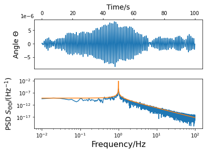
Figure 3: Monte Carlo simulation for the motion of the box. (a) Simulated time-trace of Eq. (18). (b) The PSD $S_{\Theta\Theta}$ in the lower plot is computed by FFT. Theoretically the PSD is a Lorentzian distribution which fits the simulation result well. The intrinsic frequency $\Omega_{\rm rot}$ is chosen as $2\pi\times 1$ Hz, the damping rate $\gamma_{\rm rot}$ is chosen as $10^{-10}$ Hz, the temperature is set as 300 K.

One may do a Monte Carlo simulation of the Langevin equation given in Eq. (18), shown as the upper figure of Fig. 3, and calculate the corresponding PSD by fast Fourier transform (FFT), where a Hanning window has been added to avoid the spectral leakage, shown as the lower figure of Fig. 3. We find that the analytic result Eq. (21) matches well with the numerical result.

Since the PSD of ITN is the self-convolution of $S_{\dot{\Theta}\dot{\Theta}}(\omega)$ according to Eq. (15), one can compute the PSD of the ITN driven by thermal gas collisions with the PSD given by Eq. (21) as

$$S_{\dot{\Theta}^{2}\dot{\Theta}^{2}}(\omega)=\bar{S}\frac{4\omega^{4}+4(\gamma_{\rm rot}^{2}-3\Omega_{\rm rot}^{2})\omega^{2}+16\Omega_{\rm rot}^{4}}{(\omega^{2}+\gamma_{\rm rot}^{2})(4\gamma_{\rm rot}^{2}\omega^{2}+(\omega^{2}-4\Omega_{\rm rot}^{2})^{2})},$$ (22)

where the prefactor is given by

$$\bar{S}=\frac{4\pi\gamma_{\rm rot}(k_{B}T)^{2}}{I^{2}}.$$ (23)

Figure 4: PSD of ITN $S_{\dot{\Theta}^{2}\dot{\Theta}^{2}}(\omega)$ and angular motion PSD $S_{\Theta\Theta}(\omega)$. The parameters are chosen as $\Omega_{\rm rot}=2\pi\times 1$ Hz, $\gamma_{\rm rot}=10^{-10}$ Hz, I=10 $\rm kg\cdot m^{2}$ and T=300 K. $S_{\dot{\Theta}^{2}\dot{\Theta}^{2}}(\omega)$ is numerically orders of magnitude smaller than the value of $S_{\Theta\Theta}(\omega)$ because it has an additional $k_{B}T\sim 10^{-21}$ J factor as can be seen by comparing Eqs. (21) and  (22) (the two PSDs have the units shown on the right and left axis, respectively). The peak frequency of $S_{\dot{\Theta}^{2}\dot{\Theta}^{2}}(\omega)$ is doubled compared to $S_{\Theta\Theta}(\omega)$ as expected when computing the square of the noise 9. The dashed green and purple lines show that the theoretical expressions in Eqs. (21) and  (22) fit well the simulated PSDs.

The detailed mathematical steps are summarized in Appendix B. Fig. 4 shows the analytical result and the numerical simulation of both $S_{\Theta\Theta}(\omega)$ and $S_{\dot{\Theta}^{2}\dot{\Theta}^{2}}(\omega)$. As is shown, the magnitude of ITN is about $10^{-20}$ level smaller than $S_{\Theta\Theta}$. This is because $S_{\Theta\Theta}(\omega)$ is proportional to $k_{B}T$ but $S_{\dot{\Theta}^{2}\dot{\Theta}^{2}}(\omega)$ is proportional to $(k_{B}T)^{2}$ which contributes an additional factor $k_{B}T\sim 10^{-21}$ J.

The asymptotic behaviour of the PSD of ITN is also different from the $S_{\Theta\Theta}(\omega)$. In low frequency limit, $S_{\dot{\Theta}^{2}\dot{\Theta}^{2}}(\omega)$ behaves like $1/(\omega^{2}+\gamma_{\rm rot}^{2})$ and tends to a constant $4\pi(k_{B}T/I)^{2}/\gamma_{\rm rot}$. In high frequency region, $S_{\dot{\Theta}^{2}\dot{\Theta}^{2}}(\omega)$ decreases as $\omega^{-2}$ according to the analytic result (22).

There is also a peak of the PSD of ITN, of which the resonance frequency translates from $\Omega_{\rm rot}$ to $2\Omega_{\rm rot}$, which is a common property for a squared noise . In a small damping limit $\gamma_{\rm rot}\ll\Omega_{\rm rot}$, the peak value of $S_{\dot{\Theta}^{2}\dot{\Theta}^{2}}(\omega)$ is

$$\begin{split}S_{\dot{\Theta}^{2}\dot{\Theta}^{2}}(2\Omega_{\rm rot})&=\frac{4\pi\gamma_{\rm rot}(k_{B}T)^{2}}{I^{2}}\frac{32\Omega_{\rm rot}^{4}+16\gamma_{\rm rot}^{2}\Omega_{\rm rot}^{2}}{16\gamma_{\rm rot}^{2}\Omega_{\rm rot}^{2}(4\Omega_{\rm rot}^{2}+\gamma_{\rm rot}^{2})}\\ &\approx\frac{2\pi(k_{B}T)^{2}}{\gamma_{\rm rot}I^{2}}.\end{split}$$ (24)

The quality factor (Q-factor) of ITN can be computed according to the frequency-to-bandwidth ratio known as the full width at half maximum (FWHM). In particular, under the small-damping limit $\gamma_{\rm rot}\ll\Omega_{\rm rot}$, i.e. the high-Q case, one can compute that

$$S_{\dot{\Theta}^{2}\dot{\Theta}^{2}}(2\Omega_{\rm rot}\pm\gamma_{\rm rot})\approx\frac{\pi(k_{B}T)^{2}}{\gamma_{\rm rot}I^{2}}.$$ (25)

It suggests that the FWHM frequency is $\omega=2\Omega_{\rm rot}\pm\gamma_{\rm rot}$. Thus, the frequency bandwidth is $\Delta\omega=2\gamma_{\rm rot}$ and the Q-factor for ITN is

$$Q_{\rm ITN}=\frac{2\Omega_{\rm rot}}{2\gamma_{\rm rot}}=\frac{\Omega_{\rm rot}}{\gamma_{\rm rot}},$$ (26)

which is the same as the Q-factor of $S_{\Theta\Theta}(\omega)$.

V Dephasing Factor and Experiment Parameters Constrain

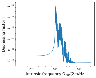
Figure 5: Dephasing factor $\Gamma$ as a function of the intrinsic torsion frequency $\Omega_{\rm rot}$. The parameters are chosen as $m_{0}=10^{-15}$ kg, $\eta=10^{4}$ T/m, $t_{a}=0.25$ s and $t_{e}=0$ s for the interferometer, and $\gamma_{\rm rot}=10^{-10}$ Hz, $I=10\,\rm kg\cdot m^{2}$ and $T=300$ K for the PSD of ITN. There is a resonance between the ITN and the transfer function with the first dominant peak at $\Omega_{\rm rot}\sim 2\pi/T_{\rm tot}\sim 2\pi\times 1$ Hz, and additional smaller peaks visible in the range upt to 10. In low frequency limit and high frequency limit, the dephasing factor $\Gamma$ is approximately independent with the intrinsic frequency $\Omega_{\rm rot}$.

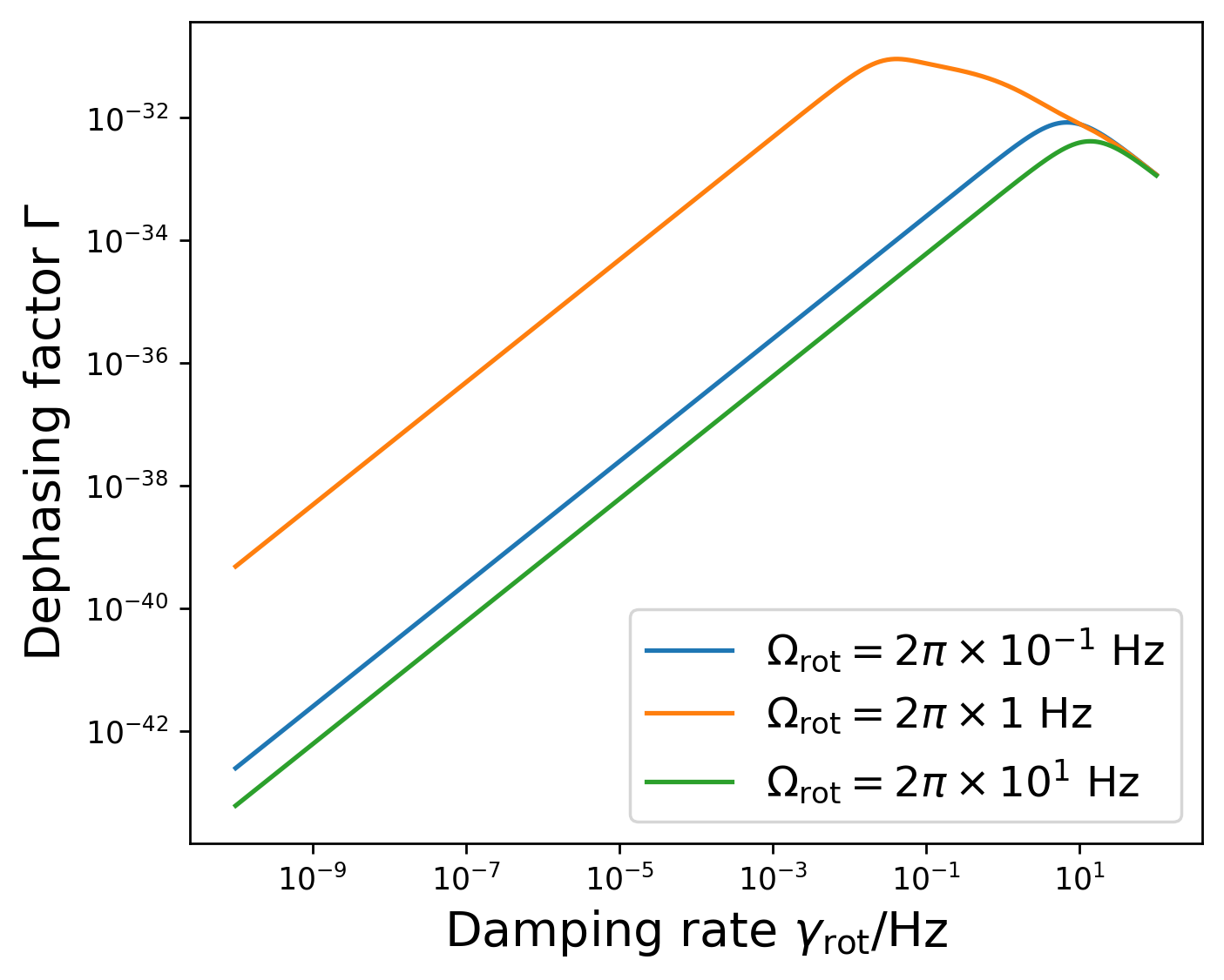
Figure 6: Dephasing factor $\Gamma$ as a function of the damping factor $\gamma_{\rm rot}$. The transfer function is given in Eq. (13) with parameters $t_{a}=0.25$ s and $t_{e}=0$ s. Three different $\Omega_{\rm rot}$ are chosen in the low rotation frequency limit (blue line), the resonance frequency condition $\Omega_{\rm rot}\sim 2\pi/T=2\pi$ Hz (orange line), and the high rotation frequency limit (green line). The dephasing $\Gamma$ is proportional to $\gamma_{\rm rot}$ when $\gamma_{\rm rot}\ll\Omega_{\rm rot}$, while it starts decreasing with respect to $\gamma_{\rm rot}$ when $\gamma_{\rm rot}$ becomes comparable or larger than $\Omega_{\rm rot}$.

Based on the result of the transfer function in Eq. (13) or Eq. (14), and the power spectrum density (22) of the inertial torsion noise, the dephasing factor $\Gamma$ can be computed through the integral in Eq. (10). As this integral is non-trivial, we employ numerical methods to compute it. It is noteworthy that a resolution of $\omega_{\rm min}=2\pi/T_{\rm tot}$ exists as a cutoff in frequency space for the numerical calculation . Physically, this cutoff indicates that a low-frequency signal or noise will not be measurable by the experiment if the total experiment time is shorter than a single period of such signal or noise.

Fig. 5 shows the dependence of $\Gamma$ on the intrinsic torsion frequency $\Omega_{\rm rot}$ of the experiment apparatus, where the parameters of $F(\omega)$ are chosen as $m_{0}=10^{-15}$ kg, $t_{a}=0.25$ s and $t_{e}=0$ s. As is shown, there is a resonance between the ITN and the transfer function near $\Omega_{\rm rot}\sim 2\pi/T_{\rm tot}=2\pi\times 1$ Hz and some harmonic resonances. Note that near the resonance peak, the precision of the numerical calculation is limited because the value is highly related to the sample points in frequency space.

When $\Omega_{\rm rot}$ is much smaller than $2\pi\times 10^{-1}$ Hz, the peak will be below the frequency cut-off $\omega_{\rm min}$, so the dephasing factor will be tiny. For an actual experiment, the low intrinsic frequency limit is expected, so the parameters $d$, $l$, $\mathbb{G}$ and $I$ in (17) have to be carefully designed to ensure $\Omega_{\rm rot}$ much smaller than the resonance frequency $2\pi/T$ of the interferometer.

When $\Omega_{\rm rot}$ is much larger than $2\pi\times 10^{0}$ Hz, $\Gamma$ becomes approximately independent on $\Omega_{\rm rot}$. Fig. 6 shows the dependence of $\Gamma$ on the damping factor $\gamma_{\rm rot}$ caused by the thermal gas molecules. Three curves with different $\Omega_{\rm rot}$ correspond to the low rotation frequency limit, the high rotation frequency limit and the resonance frequency condition $\Omega_{\rm rot}\sim 2\pi/T$. As is shown in the figure, $\Gamma$ is proportional to $\gamma_{\rm rot}$ when $\gamma_{\rm rot}\ll\Omega_{\rm rot}$, which can be read from Eq. (22). When $\gamma_{\rm rot}$ grows comparable to $\Omega_{\rm rot}$, $\Gamma$ decreases with respect to $\gamma_{\rm rot}$ increases.

Fig. 6 show the dependence of $\Gamma$ on the damping rate $\gamma_{\rm rot}$ of the gas collision. As is shown, when the damping rate is very low, i.e. $\gamma_{\rm rot}\ll\Omega_{\rm rot}$, the dephasing factor $\Gamma$ is approximately proportional to $\gamma_{\rm rot}$ because the $\bar{S}$ in Eq. (22) is proportional to $\gamma_{\rm rot}$.

However, when $\gamma_{\rm rot}$ increases after a critical point $\gamma_{\rm rot}\sim\Omega_{\rm rot}$, the dephasing factor $\Gamma$ is approximately inverse to $\gamma_{\rm rot}$. This is because the PSD of ITN at the high damping rate limit $\gamma_{\rm rot}\gg\Omega_{\rm rot}$ is approximately

$$S_{\dot{\Theta}^{2}\dot{\Theta}^{2}}(\omega)\approx\bar{S}\frac{4\omega^{4}+4\gamma_{\rm rot}^{2}\omega^{2}}{(\omega^{2}+\gamma_{\rm rot}^{2})(\omega^{4}+4\gamma_{\rm rot}^{2}\omega^{2})}\sim\frac{\bar{S}}{\gamma_{\rm rot}^{2}}.$$ (27)

Since $\bar{S}\propto\gamma_{\rm rot}$, the PSD of ITN is proportional to $\gamma_{\rm rot}^{-1}$, so the dephasing factor $\Gamma$ decreases with respect to $\gamma_{\rm rot}$. Physically it can be interpreted as an overdamped oscillator. In particular, the apparatus’s dynamical equation in Eq. (18) describes a damped oscillator under a randomly driven force. When the damping rate is larger than a critical value $\gamma_{\rm rot}>\Omega_{\rm rot}/2$, the system decays with no oscillation, known as overdamped. In the overdamped region, as the damping rate increases, the system decays to the equilibrium faster, so the random force term affects the system less. Finally, the dephasing factor $\Gamma$ decreases as the damping rate $\gamma_{\rm rot}$ increases.

A final remark on Figs. 5 and 6 we note that the dephasing factor $\Gamma$ caused by the torsion noise from gas molecules collision is negligibly tiny. Two main reasons cause this. First, the thermal motion of gas molecules is proportional to a small thermal factor $k_{B}T\sim 10^{-21}$ J. Besides, ITN is a second-order effect, so every little factor in the PSD $S_{\Theta\Theta}(\omega)$ of the experiment apparatus will be squared for the dephasing factor $\Gamma$. Combining both effects, the dephasing factor $\Gamma$ is suppressed by a highly tiny factor $(k_{B}T)^{2}\sim 10^{-42}$, such that it does not exceed $10^{-30}$ in these two plots.

VI a generic source of torsion noise

In an actual experiment, there can be a number of sources of torsion noise. To model generic noises phenomenologically we can assume the Langevin equation of the form

$$\ddot{\Theta}=-\Omega_{\rm rot}^{2}\Theta-\gamma\dot{\Theta}+\sqrt{A}\Theta_{\rm in},$$ (28)

where the dissipation rate $\gamma$ and the amplitude of the random Gaussian force $\sqrt{A}$ is determined by the experiment (and we recall that $\Omega_{\rm rot}$ is the intrinsic frequency). Te PSD of the motion of the experiment box and the ITN can be computed from the dynamical equation following analogous steps as in the previous sections:

$$S_{\Theta\Theta}(\omega) =\frac{A}{(\Omega_{\rm rot}^{2}-\omega^{2})^{2}+\gamma^{2}\omega^{2}},$$ (29)

$$S_{\dot{\Theta}^{2}\dot{\Theta}^{2}}(\omega) =A^{2}\frac{4\omega^{4}+4(\gamma^{2}-3\Omega_{\rm rot}^{2})\omega^{2}+16\Omega_{\rm rot}^{4}}{\gamma(\omega^{2}+\gamma^{2})(4\gamma^{2}\omega^{2}+(\omega^{2}-4\Omega_{\rm rot}^{2})^{2})}.$$

$S_{\dot{\Theta}^{2}\dot{\Theta}^{2}}(\omega)$ has an additional $\gamma^{-2}$ dependence in comparison to the thermal case in Eq. (22). This difference arises because the amplitude $A=2\gamma_{\rm rot}k_{B}T/I$ of the external force for the thermal noise in Eq. (18) is proportional to the damping rate $\gamma$, which does not hold for the general case considered in this section. In this case, the dependence of $\Gamma$ on the damping rate $\gamma$ is shown as Fig. 7, where the amplitude $A$ is chosen as $10^{-10}\,\rm Hz^{3}$. As is shown, $\Gamma$ is proportional to $\gamma^{-1}$ and $\gamma^{-3}$ in the underdamped region $\gamma\ll\Omega_{\rm rot}$ and overdamped region $\gamma\gg\Omega_{\rm rot}$ respectively.

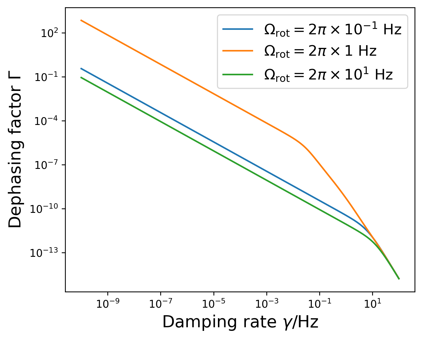
Figure 7: The relationship between $\Gamma$ and the damping factor $\gamma$ for a fixed amplitude $A=10^{-10}\,\rm Hz^{3}$. The transfer function is given in Eq. (13) with parameters $t_{a}=0.25$ s and $t_{e}=0$ s. Three different $\Omega_{\rm rot}$ are chosen as the low rotation frequency limit, the high rotation frequency limit and the resonance frequency condition $\Omega_{\rm rot}\sim 2\pi/T=2\pi$ Hz. $\Gamma$ is proportional to $\gamma^{-1}$ when $\gamma\ll\Omega_{\rm rot}$, while it decreases as a speed of $\gamma^{-3}$ in the overdamped region.

Fig. 8 shows the dependence of the dephasing factor $\Gamma$ concerning different damping rates $\gamma$ and torsion noise amplitude $A$, where the parameters are chosen as $t_{a}=0.25$ s and $t_{e}=0$ s and $\Omega_{\rm rot}=2\pi\times 1$ Hz. As is shown, $\Gamma$ increases as $A$ increases or $\gamma$ decreases. In an experiment, if one requires an upper bound of $\Gamma=0.01$, then $A$ and $\gamma$ should be chosen in the region on the left side of the cyan region in the figure. In particular, $A$ should be roughly smaller than $10^{-10}\,\rm Hz^{3}$ and $10^{-6}\,\rm Hz^{3}$ for $\gamma=10^{-10}$ Hz and $10^{-2}$ Hz.

Fig. 9 shows the upper bound of the torsion noise amplitude $A$ to obtain a dephasing factor $\Gamma$ smaller than 0.01, where the parameters are also chosen as $t_{a}=0.25$ s and $t_{e}=0$ s. As is shown, the restriction on the upper bound of $A$ is very stringent near the resonance region $\Omega_{\rm rot}\sim 2\pi/T_{\rm tot}=2\pi\times 1$ Hz and its harmonic resonance $\Omega_{\rm rot}\sim 2n\pi/T_{\rm tot}$ (with $n$ a positive integer). In particular, $A$ has to be smaller than $10^{-10}\,\rm Hz^{3}$ for $\gamma=10^{-10}$ Hz, and it has to be smaller than $10^{-8}\,\rm Hz^{3}$ for $\gamma=10^{-2}$ Hz. On the other hand, the value of $A$ is less severely constrained outside the resonance region. For a damping rate larger than $10^{-4}$ Hz, $A$ can be larger than $10^{-5}\,\rm Hz^{3}$.

In a recent simulation work [52], a relationship between the torsion noise amplitude $A$ and the superposition size $\Delta x$ has been obtained as $\Delta xA\sim 10^{-11}\,\rm m\cdot Hz^{3}$. Since the superposition size discussed in this paper is $\Delta x=a_{m}t_{a}^{2}=11.2\,\rm\mu m$, then the noise amplitude is $A\sim 10^{-6}\,\rm Hz^{3}$, which is smaller than the restricted bound $A_{\rm bound}\sim 10^{-5}\,\rm Hz^{3}$. In conclusion, as long as the damping rate is designed to be larger than $10^{-4}$ Hz and the intrinsic frequency $\Omega_{\rm rot}$ is designed outside the resonance region, the dephasing factor $\Gamma$ of the interferometer will be smaller than $0.01$.

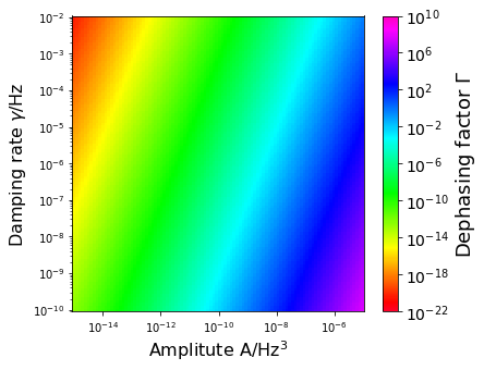
Figure 8: The dephasing factor $\Gamma$ with respect to different damping rates $\gamma$ and torsion noise amplitudes $A$. The transfer function is given by Eq. (13) with parameters $t_{a}=0.25$ s and $t_{e}=0$ s, and the intrinsic frequency is chosen as $\Omega_{\rm rot}=2\pi\times 1$ Hz. If $\Gamma$ is required to be smaller than 0.01, then the parameters should be chosen on the left side of the cyan region in the figure.

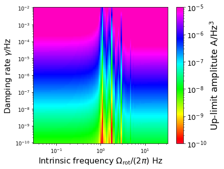
Figure 9: The upper bound of the amplitude $A$ assuming the value of the dephasing to be $\Gamma=0.01$. The transfer function is is given by Eq. (13) with parameters $t_{a}=0.25$ s and $t_{e}=0$ s. Near the resonance region $\Omega_{\rm rot}\sim 2\pi/T_{\rm tot}=2\pi\times 1$ Hz and its harmonic resonance $\Omega_{\rm rot}\sim 2n\pi/T_{\rm tot}$ (with $n$ a positive integer), the upper bound of $A$ becomes more constrained. On the other hand, the requirements on $A$ relax outside the resonance region.

VII Summary

In this paper, we investigated inertial torsion noise (ITN) in the context of matter-wave interferometry. In section II, we discussed the physical interpretation of the ITN as stochastic torsion of the suspended experimental apparatus. The consequence of such noise is a random differential phase $\delta\phi$ on the paths of the interferometer resulting in dephasing. The coherences, i.e., the off-diagonal terms of the density matrix, decay as $\mathbb{E}[\mathrm{e}^{\mathrm{i}\delta\phi}]=\mathrm{e}^{-\Gamma}$, where the decay factor is precisely the variance $\Gamma=\mathbb{E}[(\delta\phi)^{2}]$. In other words, ITN induces a loss of interferometric visibility.

The Lagrangian of the ITN is derived in Appendix A in the language of general relativity. We first constructed the rotating metric starting from Fermi normal coordinates, then computed the Lagrangian of a test mass under this metric in a non-relativistic limit. There are two terms in the Lagrangian, one of which is the centrifugal force, while the other corresponds to the Coriolis and Euler forces. Assuming the small angle approximation, and placing the superposition along the x-axis, the Lagrangian of the ITN in Eq.(5) can then be derived.

In section III, we pointed out that the decay factor $\Gamma$ can be regarded as a linear response of the interferometer to the ITN. In particular, it can be formulated as the power spectrum density of the noise $S_{\dot{\Theta}^{2}\dot{\Theta}^{2}}(\omega)$ multiplying a transfer function $F(\omega)$ in frequency space. The transfer function only relies on the trajectories of the interferometer’s two arms and is independent of the noise. The exact and approximate formulae of $F(\omega)$ are given by Eqs. (13) and (14), respectively.

In section IV, we considered a specific ITN source: the thermal gas molecule collisions on the experiment box. The motion of the box is determined by the Langevin equation, by which one can compute the PSD $S_{\Theta\Theta}(\omega)$ described in Eq. (21). According to the convolution theorem, the PSD of the ITN $S_{\dot{\Theta}^{2}\dot{\Theta}^{2}}(\omega)$ is the self-convolution of $S_{\dot{\Theta}\dot{\Theta}}(\omega)$ which relates to $S_{\Theta\Theta}(\omega)$ through Eq. (16). The calculation details of $S_{\dot{\Theta}^{2}\dot{\Theta}^{2}}(\omega)$ are summarized in Appendix B. We also did a Monte-Carlo simulation directly from the dynamical equation in Eq. (18) to double-check the analytical result. Another essential feature of ITN $S_{\dot{\Theta}^{2}\dot{\Theta}^{2}}(\omega)$ is that the peak position is doubled compared to $S_{\dot{\Theta}\dot{\Theta}}(\omega)$ because of properties of self-convolution. In addition, we showed that the Q-factor retains the usual expression as another safety check.

Finally, we studied the dephasing factor caused by ITN in section V. The dephasing factor increases significantly near the resonance region $\Omega_{\rm rot}=2n\pi/T_{\rm tot}$ for some integer $n$. It increases proportional to the damping rate $\gamma_{\rm rot}$ in the underdamped region, while it decreases with $\gamma_{\rm rot}$ in the overdamped region. As is shown in Fig. 5 and Fig. 6, the maximum value of $\Gamma$ is tiny so the dephasing caused by the thermal gas molecules collision is negligible.

For a generic source of noise described by a generalized Langevin equation (28), the dephasing factor is proportional to $\gamma_{\rm rot}^{-1}$ and $\gamma_{\rm rot}^{-3}$ in the underdamped and overdamped regions, respectively. In Fig. 9 we computed the constraints on the experimental parameters such that the dephasing factor remains smaller than $0.01$. We found that the amplitude of the noise has to be smaller than $10^{-10}\,\rm Hz^{3}$ in the resonance region, while the constrain can be relaxed to $10^{-5}\,\rm Hz^{3}$ outside the resonance region (with a damping rate larger than $10^{-4}$ Hz). Finally, we briefly compared our results with the rotational noise analysis in the context of cold atom interferometer on-board a satellite [52].

In summary, this work quantifies the dephasing in nanoparticle matter-wave interferometry arising from inertial torsion noise (ITN). We developed the general methodology as well as obtained constrains for specific sources of noise for a simple single-stage suspension forming a torsion pendulum. In future it would be interesting to perform the noise analysis for more refined suspensions such as the inverted pendulum [42] and the Roberts linkage [43].

Appendix A Lagrangian of Inertial Torsion Noise

In this appendix, we will derive the Lagrangian in Eq. (5) that gives rise to inertial torsion noise (ITN). The basic idea is firstly to construct the metric in the comoving reference frame of the experimental apparatus (Sec. A.1), and then to compute the Lagrangian of the test mass in the non-relativistic limit (Sec. A.2).

A.1 Rotating Fermi Normal Coordinates

To construct the coordinate system near the experiment, one can choose the worldline of the center of the experimental box as a fiducial time-like curve in the spacetime manifold. Based on this worldline, one can construct the Fermi normal coordinate (FNC) of the spacetime using the method of the Fermi-Walker transport. Under this coordinate, the metric can be generally written as [53]

$$\mathrm{d}s^{2}=-\left[\left(1+\frac{a^{b}x^{\prime}_{b}}{c^{2}}\right)^{2}+R_{0c0d}x^{\prime c}x^{\prime d}\right]c^{2}\mathrm{d}t^{\prime 2}-\frac{2}{3}R_{0cbd}x^{\prime c}x^{\prime d}c\mathrm{d}t^{\prime}\mathrm{d}x^{b}+\left(\delta_{bc}-\frac{1}{3}R_{bdce}x^{\prime d}x^{\prime e}\right)\mathrm{d}x^{\prime b}\mathrm{d}x^{\prime c},$$ (30)

where the indices $a,b,c,d=1,2,3$ represent the spacial coordinates. In the following, we will neglect the linear acceleration terms $\sim a^{b}$ and the Riemann tensor terms $\sim R_{abcd}$ such that the Metric in Eq. (30) reduces to the Minkowski spacetime metric in Cartesian coordinates.

To obtain the metric in a rotating reference frame we have to make an additional transformation. Rotations along the z-axis can be described by the time-dependent angle $\theta(t)$, such that the coordinates in the rotating frame are described by

$$\begin{cases}t=t^{\prime},\\ x=x^{\prime}\cos\theta(t)+y^{\prime}\sin\theta(t),\\ y=-x^{\prime}\sin\theta(t)+y^{\prime}\cos\theta(t),\\ z=z^{\prime},\end{cases}$$ (31)

where we recall the primed symbols represent the coordinates in the inertial (non-rotating) frame (see Fig. 10).

To compute the metric in the rotating coordinates one can proceed is several ways. For example, one way to simplify the calculation is to write the transformation between $(x,y)$ and $(x^{\prime},y^{\prime})$, as well as between $(\mathrm{d}x,\mathrm{d}y)$ and $(\mathrm{d}x^{\prime},\mathrm{d}y^{\prime})$, in matrix form. But here, we will offer an alternative method by exploiting the complex notation. The basic idea is to introduce a complex coordinate $w=x+\mathrm{i}y$, then the complex conjugate is $\bar{w}=x-\mathrm{i}y$, and the differentials are

$$\mathrm{d}w=\mathrm{d}x+\mathrm{i}\mathrm{d}y,\quad\quad\mathrm{d}\bar{w}=\mathrm{d}x-\mathrm{i}\mathrm{d}y,$$ (32)

with analogous expressions for the primed variables. This is a common trick to deal with 2D problems, because one can always construct a complex structure on a 2D surface through its metric to become a Riemann surface. For pedagogical material, see chapter 7 of [54].

The rotation transformation from Eq. (31), as well as its inverse, can be simply written as

$$w=w^{\prime}\mathrm{e}^{\mathrm{i}\theta(t)},\quad\quad w^{\prime}=w\mathrm{e}^{-\mathrm{i}\theta(t)},$$ (33)

where we have omitted the $t$ and $z$ coordinate transformation for brevity. We find that the differential forms are

$$\mathrm{d}w^{\prime} =\mathrm{e}^{-\mathrm{i}\theta}\mathrm{d}w^{\prime}-\mathrm{i}\dot{\theta}w^{\prime}\mathrm{e}^{-\mathrm{i}\theta}\mathrm{d}t,$$ (34)

$$\mathrm{d}\bar{w}^{\prime} =\mathrm{e}^{\mathrm{i}\theta}\mathrm{d}\bar{w}^{\prime}+\mathrm{i}\dot{\theta}\bar{w}^{\prime}\mathrm{e}^{\mathrm{i}\theta}\mathrm{d}t.$$

The considered terms $\mathrm{d}x^{\prime 2}+\mathrm{d}y^{\prime 2}=\mathrm{d}w^{\prime}\mathrm{d}\bar{w}^{\prime}$ in the original Fermi normal coordinates from Eq. (30) transform to

$$\begin{split}\mathrm{d}w^{\prime}\mathrm{d}\bar{w}^{\prime}&=(\mathrm{e}^{-\mathrm{i}\theta}\mathrm{d}w-\mathrm{i}\dot{\theta}w\mathrm{e}^{-\mathrm{i}\theta}\mathrm{d}t)(\mathrm{e}^{\mathrm{i}\theta}\mathrm{d}\bar{w}+\mathrm{i}\dot{\theta}\bar{w}\mathrm{e}^{\mathrm{i}\theta}\mathrm{d}t)\\ &=\mathrm{d}w\mathrm{d}\bar{w}-\mathrm{i}\dot{\theta}(w\mathrm{d}\bar{w}-\bar{w}\mathrm{d}w)\mathrm{d}t+\dot{\theta}^{2}w\bar{w}\mathrm{d}t^{2}\\ &=\mathrm{d}x^{2}+\mathrm{d}y^{2}+2\dot{\theta}(-x\mathrm{d}y+y\mathrm{d}x)\mathrm{d}t+\dot{\theta}^{2}(x^{2}+y^{2})\mathrm{d}t^{2},\end{split}$$ (35)

which then immediately gives the transformed metric in the rotating reference frame

$$\mathrm{d}s^{2}=-\big{(}c^{2}-\dot{\theta}^{2}(x^{2}+y^{2})\big{)}\mathrm{d}t^{2}+2\dot{\theta}(-x\mathrm{d}y+y\mathrm{d}x)\mathrm{d}t+\mathrm{d}x^{2}+\mathrm{d}y^{2}.$$ (36)

A.2 Lagrangian of Inertial Torsion Noise

Figure 10: Illustration of the inertial reference frame (labeled as $x^{\prime}$ and $y^{\prime}$) and of the rotating reference frame (labeled as $x$ and $y$), which is comoving with the experimental equipment. For simplicity, we assume that the interferometric axis (line segment connecting the light and dark blue circles) is aligned with the $x^{\prime}$ axis of the inertial frame. (a) General case when the interferometric particle is placed at angle $\phi+\theta$ with respect to the inertial reference frame. $\phi$ denotes its polar coordinate in the rotating reference frame, and $\theta$ is the angle between the inertial and rotating reference frames. (b) Special case when the interferometric axis coincides with the $x^{\prime}$-axis of the inertial reference frame. In this case, the two angles $\phi$ and $\theta$ defined in point (a) have a simple relationship $\phi=-\theta$.

Te Lagrangian of a point-like massive object is given by $L=-mc^{2}\sqrt{-\mathrm{d}s^{2}/(c^{2}\mathrm{d}t^{2})}$. Using the metric in Eq. (36) and taking the non-relativistic limit $v_{x},v_{y}\ll c$ (with $v_{x}\equiv\mathrm{d}x/\mathrm{d}t,v_{y}\equiv\mathrm{d}y/\mathrm{d}t$), we find that the Lagrangian is

$$L=-\frac{1}{2}m\dot{\theta}^{2}(x^{2}+y^{2})+m\dot{\theta}(-xv_{y}+v_{x}y),$$ (37)

where we have omitted the constant term $mc^{2}$ and the kinetic energy term $1/2m(v_{x}^{2}+v_{y}^{2})$. The term $-\frac{1}{2}m\dot{\theta}^{2}(x^{2}+y^{2})$ describes the centrifugal force. In particular, according to Euler-Lagrange equation $\frac{\mathrm{d}}{\mathrm{d}t}\left(\frac{\partial L}{\partial\dot{x}_{j}}\right)-\frac{\partial L}{\partial x_{j}}=0$, this term gives the centrifugal force $\vec{F}_{\rm cent}=m\dot{\theta}^{2}\vec{r}$. The term $m\dot{\theta}(-xv_{y}+v_{x}y)$ will give two forces, $-2m\vec{r}\times\dot{\vec{\theta}}$ and $m\vec{r}\times{\ddot{\vec{\theta}}}$, known as the Coriolis force and the Euler force, respectively. Eq. (37) is well known in the literature, and it gives rise among other things also to the Sagnac effect [55, 56, 57, 58].

The Lagrangian term $m\dot{\theta}(-xv_{y}+v_{x}y)$ can be written into polar coordinates with $x=r\cos\phi$ and $y=r\sin\phi$ (see Fig. 10(a)). If $r$ is assumed constant, then $v_{x}=-r\dot{\phi}\sin\phi$ and $v_{y}=r\dot{\phi}\cos\phi$, so this term becomes $-mr^{2}\dot{\theta}\dot{\phi}$. In the special case shown in Fig. 10(b), when the test mass is set on the $x$-axis of the inertial (non-rotating) reference frame, one may directly obtain $\phi=-\theta$. Then the Lagrangian of the Coriolis and Euler forces becomes $m\dot{\theta}^{2}r^{2}$. Therefore, the total Lagrangian of the centrifugal, the Coriolis, and the Euler forces reduces to

$$L_{\rm ITN}=\frac{1}{2}m\dot{\theta}^{2}r^{2}.$$ (38)

Finally, if the angle $\theta$ is assumed to be small, then the $y$-component is much smaller than the $x$-component in the Lagrangian. Hence making the approximation $r\approx x$ we finally obtain the ITN Lagrangian in Eq. (5).

Appendix B Calculation for PSD of ITN

In this appendix, we will calculate the PSD of the ITN arising from a thermal environment modelled by Eq. (18). As is discussed in the main text, the PSD of ITN $S_{\dot{\Theta}^{2}\dot{\Theta}^{2}}(\omega)$ is the self-convolution of the PSD of the torsion angle $S_{\dot{\Theta}\dot{\Theta}}(\omega)=\omega^{2}S_{\Theta\Theta}(\omega)$, that is,

$$\begin{split}S_{\dot{\Theta}^{2}\dot{\Theta}^{2}}(\omega)&=(S_{\dot{\Theta}\dot{\Theta}}\ast S_{\dot{\Theta}\dot{\Theta}})(\omega)\\ &=\int_{-\infty}^{\infty}(2\gamma_{\rm rot}k_{B}T/I)^{2}\frac{u^{2}}{(u^{2}-\Omega_{\rm rot}^{2})^{2}+\gamma_{\rm rot}^{2}u^{2}}\times\frac{(\omega-u)^{2}}{((\omega-u)^{2}-\Omega_{\rm rot}^{2})^{2}+\gamma_{\rm rot}^{2}(\omega-u)^{2}}\mathrm{d}u.\end{split}$$ (39)

We will use the residue theorem to calculate this integral [59]. Firstly, the poles of $S_{\Theta\Theta}(\omega)$ are

$$\omega_{1,2,3,4}=\pm\sqrt{\Omega_{\rm rot}^{2}-\gamma_{\rm rot}^{2}/4}\pm\mathrm{i}\gamma_{\rm rot}/2.$$ (40)

The positiveness of the discriminant $\Omega_{\rm rot}^{2}-\gamma_{\rm rot}^{2}/4$ will affect the positions of poles of the integrand in Eq. (39), shown in Fig. 11, of which the discriminants in sub-figures (a) and (b) are positive and negative respectively. Note that the relations $\omega_{3}=-\omega_{2}$ and $\omega_{4}=-\omega_{1}$ are used to simplify the notations in both sub-figures. However, since the integral is real-valued, both cases should have the same result. Thus, it is enough to consider the case $\Omega_{\rm rot}^{2}-\gamma_{\rm rot}^{2}/4\textgreater 0$.

Figure 11: The poles and the integral path of the integral in Eq. (39). The poles of $S_{\Theta\Theta}$ and $S_{\dot{\Theta}^{2}\dot{\Theta}^{2}}(\omega)$ are given by Eq. (40). Subfigure (a) and (b) show two cases where $\sqrt{\Omega_{\rm rot}^{2}-\gamma_{\rm rot}^{2}/4}$ is a real number and an imaginary number. Note that the relations $\omega_{3}=-\omega_{2}$ and $\omega_{4}=-\omega_{1}$ have been used to simplify the notation in both subfigures.

Then according to the residue theorem, the integral value in Eq. (39) equals the residue value of the integrand at the poles in the path shown in Fig. 11. In particular, this integral equals the summation of the residues at $\omega_{1}$, $-\omega_{2}$, $\omega+\omega_{1}$ and $\omega-\omega_{2}$ when $\omega\neq\omega_{1}+\omega_{2}$. In this case, every pole is a first-order pole. For the special case $\omega=\omega_{1}+\omega_{2}$, there are only two second-order poles $\omega_{1}$ and $\omega_{2}$, so the integral in Eq. (39) is given by these two poles. Since our purpose is to calculate the pure real-valued integral (39) and different cases of poles have to give the same result, we may focus on the case $\omega\neq\omega_{1}+\omega_{2}=2\sqrt{\Omega_{\rm rot}^{2}-\gamma_{\rm rot}^{2}/4}$, then the integrand can be written as

$$\begin{split}F(u,\omega)=A^{2}\frac{u^{2}(\omega-u)^{2}}{(u-\omega_{1})(u-\omega_{2})(u+\omega_{1})(u+\omega_{2})}\times\frac{1}{(u-(\omega-\omega_{1}))(u-(\omega-\omega_{2}))(u-(\omega+\omega_{1}))(u-(\omega+\omega_{2}))},\end{split}$$ (41)

where we denote $A=2\gamma_{\rm rot}k_{B}T/I$ for ease of writing. Then the residue values are given by

$$2\pi\mathrm{i}\underset{u=\omega_{1}}{\text{Res}}F(u) =A^{2}\frac{\pi\omega_{1}(\omega-\omega_{1})^{2}}{2\gamma_{\rm rot}\sqrt{\Omega_{\rm rot}^{2}-\gamma_{\rm rot}^{2}/4}}\times\frac{1}{\omega(\omega-\mathrm{i}\gamma_{\rm rot})(\omega-2\sqrt{\Omega_{\rm rot}^{2}-\gamma_{\rm rot}^{2}/4})(\omega-2\omega_{1})},$$ (42)

$$2\pi\mathrm{i}\underset{u=-\omega_{2}}{\text{Res}}F(u) =A^{2}\frac{\pi\omega_{2}(\omega+\omega_{2})^{2}}{2\gamma_{\rm rot}\sqrt{\Omega_{\rm rot}^{2}-\gamma_{\rm rot}^{2}/4}}\times\frac{1}{\omega(\omega-\mathrm{i}\gamma_{\rm rot})(\omega+2\sqrt{\Omega_{\rm rot}^{2}-\gamma_{\rm rot}^{2}/4})(\omega+2\omega_{2})},$$

$$2\pi\mathrm{i}\underset{u=\omega+\omega_{1}}{\text{Res}}F(u) =A^{2}\frac{(\omega+\omega_{1})^{2}\omega_{1}^{2}}{\omega(\omega+\mathrm{i}\gamma_{\rm rot})(\omega+2\omega_{1})(\omega+2\sqrt{\Omega_{\rm rot}^{2}-\gamma_{\rm rot}^{2}/4})}\times\frac{\pi}{2\omega_{1}\gamma_{\rm rot}\sqrt{\Omega_{\rm rot}^{2}-\gamma_{\rm rot}^{2}/4}},$$

$$2\pi\mathrm{i}\underset{u=\omega-\omega_{2}}{\text{Res}}F(u) =A^{2}\frac{(\omega-\omega_{2})^{2}\omega_{2}^{2}}{\omega(\omega-2\sqrt{\Omega_{\rm rot}^{2}-\gamma_{\rm rot}^{2}/4})(\omega-2\omega_{2})(\omega+\mathrm{i}\gamma_{\rm rot})}\times\frac{\pi}{2\omega_{2}\gamma_{\rm rot}\sqrt{\Omega_{\rm rot}^{2}-\gamma_{\rm rot}^{2}/4}}.$$

Finally the PSD of ITN defined as the integral (39) is

$$\begin{split}S_{\dot{\Theta}^{2}\dot{\Theta}^{2}}(\omega)&=2\pi\mathrm{i}(\underset{u=\omega_{1}}{\text{Res}}F(u)+\underset{u=-\omega_{2}}{\text{Res}}F(u)+\underset{u=\omega+\omega_{1}}{\text{Res}}F(u)+\underset{u=\omega-\omega_{2}}{\text{Res}}F(u))\\ &=A^{2}\frac{\pi}{\gamma_{\rm rot}}\frac{4\omega^{4}+4(\gamma_{\rm rot}^{2}-3\Omega_{\rm rot}^{2})\omega^{2}+16\Omega_{\rm rot}^{4}}{(\omega^{2}+\gamma_{\rm rot}^{2})(4\gamma_{\rm rot}^{2}\omega^{2}+(\omega^{2}-4\Omega_{\rm rot}^{2})^{2})}.\end{split}$$ (43)