Reducing polynomial degree by one for inner-stage operators affects neither stability nor accuracy of the Runge–Kutta discontinuous Galerkin method

Abstract.

The Runge–Kutta (RK) discontinuous Galerkin (DG) method is a mainstream numerical algorithm for solving hyperbolic equations. In this paper, we use the linear advection equation in one and two dimensions as a model problem to prove the following results: For an arbitrarily high-order RKDG scheme in Butcher form, as long as we use the $P^{k}$ approximation in the final stage, even if we drop the $k$th-order polynomial modes and use the $P^{k-1}$ approximation for the DG operators at all inner RK stages, the resulting numerical method still maintains the same type of stability and convergence rate as those of the original RKDG method. Numerical examples are provided to validate the analysis. The numerical method analyzed in this paper is a special case of the Class A RKDG method with stage-dependent polynomial spaces proposed in [11]. Our analysis provides theoretical justifications for employing cost-effective and low-order spatial discretization at specific RK stages for developing more efficient DG schemes without affecting stability and accuracy of the original method.

1. Introduction

In this paper, we perform stability analysis and optimal error estimates of a class of Runge–Kutta (RK) discontinuous Galerkin (DG) schemes for solving a linear hyperbolic equation. In these schemes, the DG operators at all inner RK stages adopt polynomial approximations of one degree lower than those of the standard RKDG schemes. The numerical method analyzed in this paper belongs to Class A of the RKDG method with stage-dependent polynomial spaces (sd-RKDG method), which we proposed in [11]. Hence, we will refer to it as the sdA-RKDG method. Its general formulation is given in (2.23) and (2.24).

1.1. RKDG method and its variant.

The DG method is a class of finite element methods that utilize discontinuous piecewise polynomial spaces. It was initially introduced by Reed and Hill in the 1970s for solving steady-state transport equations [34]. Later, in a series of works by Cockburn et al. [18, 17, 16, 14, 19], the DG method was integrated with the Runge–Kutta (RK) time discretization method for solving time-dependent hyperbolic conservation laws. The resulting fully discrete method is referred to as the RKDG method. The RKDG method features many favorable properties, such as good stability, high-order accuracy, flexibility for handling complex geometries, and capability for sharp capturing of shocks. It has become one of the mainstream numerical methods for computational fluid dynamics [20, 15].

The construction of the RKDG scheme follows the classical method-of-lines framework. For example, consider the initial value problem of the linear advection equation

$$u_{t}+\boldsymbol{\beta}\cdot\nabla u=0,\quad u=u(\boldsymbol{x},t),\quad\boldsymbol{x}\in\Omega\subset\mathbb{R}^{d},\quad d=1,2,\quad 0<t<T,$$ (1.1)

where $\boldsymbol{\beta}\in\mathbb{R}^{d}$ is a constant or a constant vector. To avoid unnecessary technicalities, we will consider a periodic rectangular domain with Cartesian meshes. If one wishes to construct a second-order RKDG scheme, the first step is to apply the DG spatial discretization to the linear advection equation (1.1), which yields a semi-discrete scheme in the form of an ordinary differential equation (ODE) system

$$\frac{\mathrm{d}}{\mathrm{d}t}u_{h}=L_{h}u_{h},$$ (1.2)

where $u_{h}$ is the semi-discrete solution, and $L_{h}$ is the DG operator. To obtain the fully discrete scheme, a second-order RK method is used for time discretization. For example, using the explicit midpoint rule with a time step size of $\tau$, we have

$$u_{h}^{(2)}= u_{h}^{n}+\frac{\tau}{2}L_{h}u_{h}^{n},$$ (1.3a)

$$u_{h}^{n+1}= u_{h}^{n}+{\tau}L_{h}u_{h}^{(2)}.$$ (1.3b)

This formulation results in a stable second-order RKDG scheme.

However, in our recent work [11], we observe that even if one uses the first-order $P^{0}$ approximation in the first stage (1.3a), the resulting numerical scheme is still stable and admits optimal accuracy. Let $\widetilde{L}_{h}$ be the $P^{0}$ approximation of $L_{h}$. In other words, it is the $P^{1}$-DG operator without the evaluation of linear modes. See (2.17) for the rigorous setup. Then the scheme

$$u_{h}^{(2)}= u_{h}^{n}+\frac{\tau}{2}\widetilde{L}_{h}u_{h}^{n},$$ (1.4a)

$$u_{h}^{n+1}= u_{h}^{n}+{\tau}L_{h}u_{h}^{(2)}$$ (1.4b)

is still stable under the usual Courant–Friedrichs–Lewy (CFL) condition and maintains second-order accuracy. (1.4) is an example of the sdA-RKDG scheme (2.23).

In the implementation of the RKDG scheme (1.3), one needs to evaluate the second-order $P^{1}$-DG operator $L_{h}$ twice, while in the implementation of the sdA-RKDG scheme (1.4), one only needs to evaluate a first-order $P^{0}$-DG operator once and a second-order $P^{1}$-DG operator once. The ratio of the total numbers of polynomial coefficients one needs to evaluate in (1.4) and (1.3) is $d+2:2d+2$, which is $75\%$ in one dimension (1D, also for one-dimensional) and about $66.7\%$ in two dimensions (2D, also for two-dimensional). As one can see, in (1.4), by breaking the method-of-lines structure and allowing DG operators with reduced polynomial order, we can obtain a more efficient numerical scheme without sacrificing stability and optimal order of accuracy.

1.2. An ODE argument for optimal accuracy.

The stability and accuracy of (1.4) were analyzed through the von Neumann approach in [11]. For an intuitive explanation of the optimal order of accuracy, although not rigorous, the following hand-waving argument may offer some insights. Indeed, one can consider $\widetilde{L}_{h}$ as a first-order perturbation of the second-order operator $L_{h}$, namely, $\widetilde{L}_{h}=L_{h}+\mathcal{O}(h)$, with $h$ being the spatial mesh size. Substituting this expression into (1.4), one obtains

$$u_{h}^{n+1}=\left(I+\tau L_{h}+\frac{\tau^{2}}{2}L_{h}^{2}\right)u_{h}^{n}+\mathcal{O}(\tau^{2}h).$$ (1.5)

Note that without the term $\mathcal{O}(\tau^{2}h)$, (1.5) gives back the scheme (1.3). The perturbation in the first stage operator, after being multiplied by $\tau$ twice, contributes only to a third-order local truncation error $\mathcal{O}(\tau^{2}h)$ under the usual time step constraint $\tau\leq Ch$, which does not affect the global-in-time second-order convergence.

Indeed, the above analysis of the low-order (or low-precision) perturbation of RK stages has been systematically studied in the context of ODEs by Grant in [24]. See also [8, 7]. As a special case of Grant’s work, we have the following observation: For an RK method in Butcher form of $r$th order, if one perturbs all inner-stage operators by $\mathcal{O}(\varepsilon)$ and leaves the final stage untouched, the resulting perturbed RK method admits the local truncation error $\mathcal{O}(\tau^{r+1})+\mathcal{O}(\varepsilon\tau^{2})$. Thanks to the extra $\tau$ and the fact $\tau\sim h$, one can take the perturbation as large as $\varepsilon\sim h^{k}$ at inner stages and still achieve optimal accuracy in the global error $\mathcal{O}(\tau^{r}+h^{k+1})$. In other words, for high-order RK schemes in Butcher form, reducing the accuracy of the inner-stage operators by one may not affect the overall convergence rate. In [10], we used this idea to develop an RKDG method with compact stencils. In [11], we further explored this idea and developed the sd-RKDG method, and Grant’s theory may relate to the performance of the Class A schemes of the sd-RKDG method.

1.3. Limitations of the existing analysis.

Although the von Neumann analysis in [11] and the local truncation error analysis in [24] shed light on the stability and accuracy of the sdA-RKDG schemes, these analyses have essential limitations and should not be considered as a complete theoretical justification for the sdA-RKDG method. The von Neumann analysis only applies to linear problems with constant coefficients on periodic domains. Moreover, this approach requires to analyze matrix eigenvalues, which are difficult to obtain analytically for high-order schemes or in multiple dimensions. The local truncation error analysis of the perturbed RK method relies on the assumption that the ODE operator has bounded derivatives. However, in the context of the fully discrete schemes for partial differential equations (PDEs), the operators $L_{h}$ and $\widetilde{L}_{h}$ scale inversely proportional to the mesh size $h$, which violates the essential assumptions in numerical ODE analysis as the limit $h\to 0$ is approached. Indeed, in the design of sd-RKDG schemes [11], we have encountered cases where the local truncation error analysis mismatches the actual convergence rate for the sd-RKDG schemes. It may indicate that the ODE approach in [24] may not fully explain the numerical performance of the PDE solvers. In fact, for the error estimates in this paper, a very different argument will be used for the proof.

1.4. Literature review.

The classical approach for analyzing finite element schemes is through an energy-type argument, in which one exploits the weak formulation of the numerical scheme and derives norm estimates by taking appropriate test functions [43, 2, 6]. In terms of the DG method for hyperbolic problems, although there are many earlier works on the analysis of the DG schemes for the steady-state transport equations [27, 26, 31, 5] or semi-discrete DG schemes for the time-dependent hyperbolic conservation laws [25, 35], a systematic stability and error analysis was not readily available until recently. In [49, 51], Zhang and Shu analyzed the stability and error estimates of the second- and third-order RKDG schemes. These works also relate to [6] on the study of the stabilized finite element methods by Burman et al. and also to [42] on the stability analysis of the third-order RK method for generic linear semi-negative problems by Tadmor. The analysis of RKDG schemes of higher order was hindered by the stability analysis of the fourth-order RK scheme for some time, which was then resolved in [37]. With the experience on the fourth-order RK method [37, 32], the stability analysis for both the RK method for generic linear semi-negative problems and for the RKDG method was extended to very high order [38, 48, 44, 40]. The stability theory also facilitated the error estimates of the RKDG schemes. See [44, 46, 39, 1, 45].

1.5. Challenges, main ideas, and main results.

In this paper, we perform stability analysis and optimal error estimates of the sdA-RKDG method for the linear advection equation in both 1D and 2D. The analysis is conducted for schemes of arbitrarily high order.

The major challenge in the analysis is that the sdA-RKDG method goes beyond the classical method-of-lines framework and involves two different spatial operators within each time step. While in most previous works, the fully discrete analysis typically only involves the same spatial operator across all stages. From this perspective, the challenge in the analysis of the sdA-RKDG method shares similarities with the analysis of the Lax–Wendroff DG method [36] and the RKDG method with stage-dependent numerical fluxes [45]. However, they are also very different in the sense that [36, 45] mainly involve different flux terms, while the sdA-RKDG method involves operators associated with different polynomial spaces. This difference presents significant challenges: For the sdA-RKDG method, even the solution $u_{h}^{n}$ itself may not be in the test function space that defines the low-order operator $\widetilde{L}_{h}$ in (2.17).

The main idea to overcome these difficulties is the following. We will work on the strong form, instead of the weak bilinear form, of the sdA-RKDG scheme. We note that $\widetilde{L}_{h}=(I-\Pi_{\perp})L_{h}$, where $(I-\Pi_{\perp})$ is the $L^{2}$ projection to the $P^{k-1}$ space (and $\Pi_{\perp}$ is the projection to the orthogonal complement of the $P^{k-1}$ space in the $P^{k}$ space). Therefore, the $\widetilde{L}_{h}$ operator can be formally embedded into the usual $P^{k}$-DG space, which avoids the complication of working with different spaces. For the stability analysis, we reformulate the sdA-RKDG scheme as the standard RKDG scheme plus some perturbation terms consisting of compositions of $L_{h}$ and $\Pi_{\perp}$. The main results for the stability analysis are summarized below.

• In each time step, the $L^{2}$ energy of the sdA-RKDG solution can be bounded by that of the standard RKDG solution along with some vanishing jump terms (Lemma 3.8). Through this energy estimate, one can deduce that the sdA-RKDG method retains the same type of stability as the standard RKDG method (Theorem 3.9).

For the error estimates, we derive the error equation in a compact form. We design a class of special projection operators so that certain remainder terms in the error equation can be appropriately controlled or eliminated. These projection operators differ from those found in classical finite element literature, as their construction also incorporates the time step size $\tau$. The main results for the error analysis are summarized below.

• We construct a class of projection operators that are well-defined and admit the optimal approximation estimate under the usual CFL condition (Lemmas 4.7 and 4.11). With these new projection operators, we prove the optimal error estimates of the sdA-RKDG schemes (Theorems 4.6 and 4.10).

We want to remark that the error estimates in this paper are written in a different language from that in previous works [49, 50, 44, 46], where the analysis is conducted using the multi-stage weak form of the RKDG schemes. To leverage the stability estimates in Section 3, the error estimates in this paper are performed under the compact strong form of the sdA-RKDG method with all stages combined. The language in this paper is more similar to that in the classical work by Brenner et al. [3]. However, despite the differences in notations at first glance, the two approaches are indeed closely interrelated. See Appendix A.

1.6. Significance and novelty.

In this work, we utilize the RKDG method for the linear advection equation as an illustrative example. Through systematic and rigorous analysis, we demonstrate the feasibility of employing cost-effective and coarse spatial discretization at specific RK stages for developing a numerical scheme that is highly efficient while maintaining the stability and accuracy of the original method. Our findings provide valuable insights, laying the groundwork for future research of fully discrete RK solvers for time-dependent PDEs involving low-order perturbed spatial operators. The ideas and techniques presented in this paper may extend beyond DG spatial discretization, encompassing other methods such as the continuous finite element method and the spectral method.

Below, we summarize our major theoretical novelties and contributions.

• This paper exemplifies a novel framework for conducting stability and error analysis for numerical PDE schemes beyond the method of lines.

• In the stability analysis, we establish energy estimates bounding the $L^{2}$ norm of the high-order DG modes by jump terms. See Lemmas 3.5, 3.7, and 3.14. These estimates indicate that filtering out high-order DG modes may have effects comparable to imposing jump penalties. The modal filter and jump penalty are two very commonly used approaches for stabilizing DG schemes. Our estimates reveal the inherent connections between the two stabilization approaches and demonstrate the stability effects in the fully discrete setting.

• In the error estimates, by adopting the compact strong form in the analysis, we gain further insights into the error accumulation through the RK iteration.

  1. Firstly, through the error equation (4.54) and its norm estimates (4.55), one can directly see how the norm increment or decrement of the RK scheme can affect the growth of the projected error $\xi_{h}^{n}$, which bridges the error estimates of the RKDG scheme with recent works on the norm estimates of the RK method for homogeneous linear semi-negative problems [42, 37, 32, 38, 40].

  2. Secondly, by writing the error equation in the compact strong form, one can conveniently identify the remainder terms after a complete time step. It facilitates the design of novel projection operators (and typically, global projection operators) with information both in space and time for optimal error estimates.

1.7. Organization of the paper.

As we are performing a systematic and unified analysis for sdA-RKDG schemes of arbitrarily high order, the paper unavoidably becomes lengthy and technical. Below, we explain the organization and provide tips on reading the paper.

• Since there are no significant differences in the 1D and 2D analyses, we use unified notations for both cases and conduct the analysis simultaneously. However, to avoid being distracted by the complications in the 2D notations, it would be helpful for readers to concentrate on the 1D case when verifying propositions and lemmas.

• While the scope of the paper focuses on generic high-order sdA-RKDG schemes, to enhance readability, we begin each section on stability and error analysis with the second-order case (1.4). The lemmas introduced in the analysis of the second-order scheme will serve as the base case for extension to higher-order schemes. To avoid being confused by the general high-order cases, we suggest the readers to skip Sections 3.2.4, 4.3.2, 6.2, and 6.6 in the first-round reading.

• The key to the stability analysis is to acquire estimates in Lemmas 3.5 and 3.14, and the key to the optimal error estimates is to construct projection operators in Lemmas 4.7 and 4.11. The proofs of these lemmas are technical. To avoid disrupting the flow of the paper, we postpone these proofs to Section 6 near the end of the paper.

The rest of the paper is organized as follows. In Section 2, we introduce the notations and preliminaries. Sections 3 and 4 provide stability analysis and optimal error estimates, respectively. In each of these sections, we begin with the second-order case before presenting results for higher-order cases. Section 5 presents numerical examples to verify our theoretical analysis, while Section 6 contains proofs of several technical lemmas. Finally, conclusions are given in Section 7.

2. Notations and preliminaries

2.1. DG spatial discretization

2.1.1. 1D case

Consider the 1D linear advection equation

$$u_{t}+\beta u_{x}=0,\quad u=u(x,t),\quad x\in\Omega\subset\mathbb{R},\quad 0<t<T.$$ (2.1)

We assume the periodic boundary condition, and $\beta>0$ is a positive constant.

Let $\Omega_{h}=\{I_{i}\}_{i=1}^{N}$, with $I_{i}=(x_{i-1/2},x_{i+1/2})$ be a quasi-uniform mesh partition of $\Omega$. We denote by $h_{i}=x_{i+1/2}-x_{i-1/2}$ and $h=\max_{i=1,\cdots,N}h_{i}$. The finite element space of the DG method is chosen as

$${V}_{h}^{\ell}=\{v\in L^{2}(\Omega):v|_{I_{i}}\in{P}^{\ell}(I_{i})\quad\forall i=1,\cdots,N\},$$ (2.2)

where ${P}^{\ell}(I_{i})$ is the linear space for polynomials on $I_{i}$ of degree less than or equal to $\ell$.

Let $\left(w,v\right)=\sum_{i=1}^{N}\left(w,v\right)_{I_{i}}=\sum_{i=1}^{N}\int_{I_{i}}wv\mathrm{d}x$ be the $L^{2}$ inner product and $\left\|v\right\|=\sqrt{\left(v,v\right)}$ be the $L^{2}$ norm on $\Omega_{h}$. We denote by $L_{h}$ the DG approximation of the operator $L=-\beta\partial_{x}$ with the upwind flux, where $L_{h}:{V}_{h}^{k}\to{V}_{h}^{k}$ is defined such that

$$\left(L_{h}w_{h},v_{h}\right)=\beta\left(w_{h},(v_{h})_{x}\right)-\beta\sum_{i=1}^{N}\left((w_{h}^{-}v_{h}^{-})_{i+\frac{1}{2}}-(w_{h}^{-}v_{h}^{+})_{i-\frac{1}{2}}\right)\qquad\forall v_{h}\in{V}_{h}^{k}.$$ (2.3)

Here $(v_{h}^{\pm})_{i+1/2}=\lim_{\varepsilon\to 0^{\pm}}v_{h}(x_{i+1/2}+\varepsilon)$ is the limit of $v_{h}$ from the left or the right of $x_{i+1/2}$.

Moreover, we introduce the following notations associated with jumps and traces.

$$[v_{h}]=v_{h}^{+}-v_{h}^{-},\quad\left[w_{h},v_{h}\right]=\beta\sum_{i=1}^{N}([w_{h}][v_{h}])_{i+1/2},\quad\left\llbracket v_{h}\right\rrbracket=\left[v_{h},v_{h}\right]^{1/2}$$ (2.4)

and

$$\left\|v_{h}\right\|_{\Gamma}=\left(\beta\sum_{i=1}^{N}\left((v_{h}^{-})_{i+1/2}^{2}+(v_{h}^{+})_{i+1/2}^{2}\right)\right)^{1/2}.$$ (2.5)

2.1.2. 2D case

Consider the 2D linear advection equation

$$u_{t}+\beta^{x}u_{x}+\beta^{y}u_{y}=0,\quad u=u(x,y,t),\quad(x,y)\in\Omega\subset\mathbb{R}^{2},\quad 0<t<T.$$ (2.6)

To avoid unnecessary technicalities, we consider a rectangular domain with periodic boundary conditions. $\beta^{x}>0$ and $\beta^{y}>0$ are positive constants.

Let $\Omega_{h}=\{K_{ij}\}$ be a partition of the domain, where $K_{ij}=(x_{i-1/2},x_{i+1/2})\times(y_{j-1/2},y_{j+1/2})$, $i=1,\cdots,N_{x}$ and $j=1,\cdots,N_{y}$. We denote by $h_{x}^{i}=x_{i+1/2}-x_{i-1/2}$ and $h_{y}^{j}=y_{j+1/2}-y_{j-1/2}$. Then we set

$${V}_{h}^{\ell}=\{v\in L^{2}(\Omega):v|_{K_{ij}}\in{P}^{\ell}(K_{ij})\quad\forall i,j\}$$ (2.7)

where ${P}^{\ell}(K_{ij})$ is the linear space for polynomials on $K_{ij}$ of degree less than or equal to $\ell$.

Let $\left(w,v\right)=\sum_{i=1}^{N_{x}}\sum_{j=1}^{N_{y}}\left(w,v\right)_{K_{ij}}=\sum_{i=1}^{N_{x}}\sum_{j=1}^{N_{y}}\int_{K_{ij}}wv\mathrm{d}x\mathrm{d}y$ be the $L^{2}$ inner product and $\left\|v\right\|=\sqrt{\left(v,v\right)}$ be the $L^{2}$ norm on $\Omega_{h}$. We denote by $L_{h}$ the DG approximation of the operator $L=-\beta^{x}\partial_{x}-\beta^{y}\partial_{y}$, where $L_{h}:V_{h}^{k}\to V_{h}^{k}$ is defined such that for all $v_{h}\in V_{h}^{k}$,

$$\left(L_{h}w_{h},v_{h}\right)=\left(w_{h},\beta^{x}(v_{h})_{x}+\beta^{y}(v_{h})_{y}\right)$$ (2.8)

$$-\sum_{i=1}^{N_{x}}\sum_{j=1}^{N_{y}}\int_{x_{i-\frac{1}{2}}}^{x_{i+\frac{1}{2}}}\beta^{y}\left(w_{h}\left(x,y_{j+\frac{1}{2}}^{-}\right)v_{h}\left(x,y_{j+\frac{1}{2}}^{-}\right)-w_{h}\left(x,y_{j-\frac{1}{2}}^{-}\right)v_{h}\left(x,y_{j-\frac{1}{2}}^{+}\right)\right)\mathrm{d}x$$

$$-\sum_{i=1}^{N_{x}}\sum_{j=1}^{N_{y}}\int_{y_{j-\frac{1}{2}}}^{y_{j+\frac{1}{2}}}\beta^{x}\left(w_{h}\left(x_{i+\frac{1}{2}}^{-},y\right)v_{h}\left(x_{i+\frac{1}{2}}^{-},y\right)-w_{h}\left(x_{i-\frac{1}{2}}^{-},y\right)v_{h}\left(x_{i-\frac{1}{2}}^{+},y\right)\right)\mathrm{d}y.$$

Here the superscript $-$ ($+$) indicates the limit from the left or below (right or above).

Moreover, we introduce the following notations associated with jumps and traces.

$$[v_{h}]_{i,j+\frac{1}{2}}= v_{h}\left(x,y_{j+\frac{1}{2}}^{+}\right)-v_{h}\left(x,y_{j+\frac{1}{2}}^{-}\right),$$ (2.9)

$$[v_{h}]_{i+\frac{1}{2},j}= v_{h}\left(x_{i+\frac{1}{2}}^{+},y\right)-v_{h}\left(x_{i+\frac{1}{2}}^{-},y\right),$$ (2.10)

$$\left[w_{h},v_{h}\right]= \sum_{i=1}^{N_{x}}\sum_{j=1}^{N_{y}}\left(\int_{x_{i-\frac{1}{2}}}^{x_{i+\frac{1}{2}}}\beta^{y}\left([w_{h}][v_{h}]\right)_{i,j+\frac{1}{2}}\mathrm{d}x+\int_{y_{j-\frac{1}{2}}}^{y_{j+\frac{1}{2}}}\beta^{x}\left([w_{h}][v_{h}]\right)_{i+\frac{1}{2},j}\mathrm{d}y\right),$$ (2.11)

$$\left\llbracket v_{h}\right\rrbracket= \left[v_{h},v_{h}\right]^{\frac{1}{2}},$$ (2.12)

$$\left\|v_{h}\right\|_{\Gamma}= \left(\sum_{i=1}^{N_{x}}\sum_{j=1}^{N_{y}}\beta^{y}\int_{x_{i-\frac{1}{2}}}^{x_{i+\frac{1}{2}}}\left(v_{h}\left(x,y_{j+\frac{1}{2}}^{-}\right)\right)^{2}+\left(v_{h}\left(x,y_{j+\frac{1}{2}}^{+}\right)\right)^{2}\mathrm{d}x\right.$$

$$\left.+\sum_{i=1}^{N_{x}}\sum_{j=1}^{N_{y}}\beta^{x}\int_{y_{j-\frac{1}{2}}}^{y_{j+\frac{1}{2}}}\left(v_{h}\left(x_{i+\frac{1}{2}}^{-},y\right)\right)^{2}+\left(v_{h}\left(x_{i+\frac{1}{2}}^{+},y\right)\right)^{2}\mathrm{d}y\right)^{\frac{1}{2}}.$$ (2.13)

2.1.3. Notations for both 1D and 2D cases.

Throughout the paper, we use $C$, possibly with subscripts, for a generic constant independent of the time step size $\tau$ and the spatial mesh size $h$.

Consider a mesh partition of the domain $\Omega_{h}=\{K\}$. The DG space is set as

$$V_{h}^{\ell}=\{v\in L^{2}(\Omega):v|_{K}\in P^{\ell}(K)\quad\forall K\in\Omega_{h}\}.$$ (2.14)

The $P^{k}$-DG operator $L_{h}:V_{h}^{k}\to V_{h}^{k}$ is defined in (2.3) and (2.8). It can be shown that $L_{h}$ is a semi-negative operator, as explained in Proposition 2.1. For more details, see [51, 12, 48].

Proposition 2.1 (Negative semi-definiteness of the DG operator).

In both 1D and 2D,

$$\left[w_{h},v_{h}\right]=-\left((L_{h}+L_{h}^{\top})w_{h},v_{h}\right)\quad\forall w_{h},v_{h}\in V_{h}^{k}.$$ (2.15)

and $\left\llbracket v_{h}\right\rrbracket^{2}=-\left((L_{h}+L_{h}^{\top})v_{h},v_{h}\right)\geq 0$ for all $v_{h}\in V_{h}^{k}$.

The semi-discrete $P^{k}$-DG scheme can be written as a semi-negative ODE system

$$\frac{\mathrm{d}}{\mathrm{d}t}u_{h}=L_{h}u_{h}.$$ (2.16)

In the sdA-RKDG scheme, we also need the $P^{k-1}$-DG operator, which is defined as $\widetilde{L}_{h}:V_{h}^{k}\to V_{h}^{k-1}$ such that (please pay attention to the test function space)

$$\left(\widetilde{L}_{h}w_{h},v_{h}\right)=\left(L_{h}w_{h},v_{h}\right)\quad\forall v_{h}\in{V}_{h}^{k-1}.$$ (2.17)

Let $V_{h}^{\perp}$ be the orthogonal complement of $V_{h}^{k-1}$ in $V_{h}^{k}$. We introduce the operators

$$\Pi:L^{2}(\Omega)\to V_{h}^{k},\quad\Pi_{k-1}:L^{2}(\Omega)\to V_{h}^{k-1},\quad\text{and}\quad\Pi_{\perp}:L^{2}(\Omega)\to V_{h}^{\perp}$$ (2.18)

for the $L^{2}$ projection to $V_{h}^{k}$, $V_{h}^{k-1}$, and $V_{h}^{\perp}$, respectively. It can be seen that the $P^{k-1}$-DG operator $\widetilde{L}_{h}:V_{h}^{k}\to V_{h}^{k-1}$ satisfies

$$\widetilde{L}_{h}=\Pi_{k-1}L_{h}=(I-\Pi_{\perp})L_{h}$$ (2.19)

and can be formally regarded as an operator on $V_{h}^{k}$, namely, $\widetilde{L}_{h}:V_{h}^{k}\to V_{h}^{k}$.

With the inverse estimate, it can be seen that

$$\left\llbracket v_{h}\right\rrbracket\leq C\left\|v_{h}\right\|_{\Gamma}\leq Ch^{-\frac{1}{2}}\left\|v_{h}\right\|\quad\forall v\in V_{h}^{k}.$$ (2.20)

Then using the definition of $L_{h}$, we have $\left\|L_{h}v_{h}\right\|\leq Ch^{-1}\left\|v_{h}\right\|$ for all $v_{h}\in V_{h}^{k}$, or equivalently, $\left\|L_{h}\right\|\leq Ch^{-1}$. Let us denote by $\lambda=\tau/h$. Hence we have $\tau\left\|\widetilde{L}_{h}\right\|=\tau\left\|\Pi_{k-1}L_{h}\right\|\leq\tau\left\|L_{h}\right\|\leq C\lambda$. Without loss of generality, we assume $\lambda\leq 1$ throughout the paper.

2.2. RKDG and sdA-RKDG schemes

The standard RKDG scheme in Butcher form is written as

$$u_{h}^{(i)}= u_{h}^{n}+\tau\sum_{j=1}^{i-1}a_{ij}L_{h}u_{h}^{(j)},\qquad i=1,2,\cdots,s,$$ (2.21a)

$$u_{h}^{n+1}= u_{h}^{n}+\tau\sum_{i=1}^{s}b_{i}L_{h}u_{h}^{(i)}.$$ (2.21b)

We will only consider explicit RK schemes in this paper and assume $a_{ij}=0$ if $j\geq i$. In this case, for an $r$th-order RK method, the RK operator for the linear autonomous problem (2.16) should match its stability polynomial, and can hence be written in a compact form as

$$u_{h}^{n+1}=R_{h}u_{h}^{n}:=\sum_{i=0}^{s}\alpha_{i}(\tau L_{h})^{i}u_{h}^{n}=\left(I+\tau L_{h}\sum_{i=1}^{s}\alpha_{i}(\tau L_{h})^{i-1}\right)u_{h}^{n},$$ (2.22)

where $\alpha_{i}=(i!)^{-1}\text{ for }i=0,1,\cdots,r$.

In the sdA-RKDG scheme, we replace the $P^{k}$-DG operator at inner stages by the $P^{k-1}$-DG operator $\widetilde{L}_{h}$. Then the scheme can be written as

$$u_{h}^{(i)}= u_{h}^{n}+\tau\sum_{j=1}^{i-1}a_{ij}\widetilde{L}_{h}u_{h}^{(j)},\qquad i=1,2,\cdots,s,$$ (2.23a)

$$u_{h}^{n+1}= u_{h}^{n}+\tau\sum_{i=1}^{s}b_{i}L_{h}u_{h}^{(i)}.$$ (2.23b)

It yields the compact form

$$u_{h}^{n+1}=\widetilde{R}_{h}u_{h}^{n}:=\left(I+\tau L_{h}\sum_{i=1}^{s}\alpha_{i}(\tau\widetilde{L}_{h})^{i-1}\right)u_{h}^{n},$$ (2.24)

where $\alpha_{i}=(i!)^{-1}\text{ for }i=0,1,\cdots,r$. In other words, we only use the $P^{k}$-DG operator $L_{h}$ on the very left, and we use the $P^{k-1}$-DG operator $\widetilde{L}_{h}$ at all other places.

When there is no confusion, we will refer to (2.22) as an RK$r$DG$k$ scheme, and (2.24) as an sdA-RK$r$DG$k$ scheme.

Remark 2.2 (Efficiency).

Note that for linear problems, both (2.22) and (2.24) can be efficiently evaluated using Horner’s method as:

$$u_{h}^{n+1}=\left(I+\tau L_{h}\left(\alpha_{1}I+Z_{h}\left(\alpha_{2}I+Z_{h}\left(\alpha_{3}I+\cdots+Z_{h}\left(\alpha_{s-1}I+\alpha_{s}Z_{h}\right)\right)\right)\right)\right)u_{h}^{n},$$ (2.25)

where $Z_{h}=\tau L_{h}$ for the RKDG scheme and $Z_{h}=\tau\widetilde{L}_{h}$ for the sdA-RKDG scheme. Both methods can be evaluated with $s$ matrix multiplications. Typically, for $d\geq 2$ and upwind DG schemes, (2.25) requires even fewer floating-point multiplications than directly multiplying $R_{h}$ or $\widetilde{R}_{h}$ assembled beforehand.

Since the ratio of the total degrees of freedom for $P^{k-1}$ and $P^{k}$ polynomials is $k:d+k$, the ratio of computational operations involved in $\widetilde{L}_{h}$ and $L_{h}$ is approximately $k:d+k$. Hence, in each time step, the computational operations involved in the sdA-RKDG and the sd-RKDG methods are approximately $(s-1)k+d+k:s(d+k)=sk+d:s(k+d)$. In the extreme case of solving high-dimensional problems with $d\gg k$, this ratio is approximately $1:s$.

In Section 5.4, we compare the efficiency of the sdA-RKDG and the RKDG schemes in 2D by analyzing the number of nonzero entries in the matrices involved in each time iteration. We present results in Table 5.8. The computational cost of the sdA-RKDG scheme ranges from approximately $70.6\%$ to $86.1\%$ of that of the RKDG method for $2\leq s=r=k+1\leq 9$.

Remark 2.3 (RK method in Butcher form).

The analysis in this paper only considers the RK method in Butcher form and may not be directly applicable to the RK method in Shu–Osher form (also known as the strong-stability-preserving form [23, 22]), unless a transformation is performed to rewrite a Shu–Osher form RK method back into the Butcher form. This is because our analysis relies on the following crucial fact: The operator on the very left of (2.24) is the full DG operator $L_{h}$, and does not involve the reduced operator $\widetilde{L}_{h}$. Altering the inner stages of an RKDG scheme in Shu–Osher form could result in having $\widetilde{L}_{h}$ present in the final stage, thereby disrupting the structure we have discussed. Such a method could yield a Class B sd-RKDG method, as described in [11], which maintains optimal convergence for problems without sonic points but could suffer from accuracy degeneracy when sonic points occur.

We note that the RK method in Butcher form is also widely used for numerical solutions for hyperbolic conservation laws. See, for example, [30, 33, 21].

3. Stability analysis

3.1. Stability analysis: the second-order case

3.1.1. Main result

In this section, we prove the stability of the sdA-RK2DG1 scheme (1.4).

Theorem 3.1 (Stability of sdA-RK2DG1).

The sdA-RK2DG1 scheme (1.4) is monotonically stable, namely, $\left\|u_{h}^{n+1}\right\|\leq\left\|u_{h}^{n}\right\|$ for $\lambda\ll 1$.

3.1.2. Preliminaries: stability of the RK2DG1 scheme

Before proceeding to prove Theorem 3.1, we first recall the stability analysis of the standard RK2DG1 scheme (1.3), which can be written in the compact form as

$$u_{h}^{n+1}=\left(I+\tau L_{h}+\frac{\tau^{2}}{2}L_{h}^{2}\right)u_{h}^{n}:=R_{h,2}u_{h}^{n}.$$ (3.1)

The energy estimate of the RK2 scheme can be found in many previous works. See, for example, [51, 36, 38, 48].

Proposition 3.2 (Energy identity of RK2).

$$\left\|R_{h,2}w_{h}\right\|^{2}=\left\|w_{h}\right\|^{2}+\frac{\tau^{4}}{4}\left\|L_{h}^{2}w_{h}\right\|^{2}-\tau\left\llbracket w_{h}\right\rrbracket^{2}-{\tau^{2}}\left[w_{h},L_{h}w_{h}\right]-\frac{\tau^{3}}{2}\left\llbracket L_{h}w_{h}\right\rrbracket^{2}.$$ (3.2)

In general, the right hand side of (3.2) may not be bounded by $\left\|w_{h}\right\|^{2}$ appropriately. Indeed, it is known that the RK$2$DG$k$ method is unstable under the usual CFL condition if $k\geq 2$ [20]. But when coupled with $P^{1}$ elements, the RK2DG1 method is stable due to the following norm estimate, whose proof can be found in [36, 48, 47].

Proposition 3.3 (Bounding high-order DG derivatives hy jumps).

With $P^{1}$ elements,

$${\tau^{4}}\left\|L_{h}^{2}w_{h}\right\|^{2}\leq C\left(\tau\lambda^{3}\left\llbracket w_{h}\right\rrbracket^{2}+\tau^{3}\lambda\left\llbracket L_{h}w_{h}\right\rrbracket^{2}\right).$$ (3.3)

Simple algebra shows that $\tau^{2}\left[w_{h},L_{h}w_{h}\right]\leq 3/4\cdot\tau\left\llbracket w_{h}\right\rrbracket^{2}+1/3\cdot\tau^{3}\left\llbracket L_{h}w_{h}\right\rrbracket^{2}$, and hence this cross term can be absorbed by the negative jump terms in (3.2). Thus, Propositions 3.2 and 3.3 together imply the following stability results for the RK2DG1 scheme (3.1).

Proposition 3.4 (Monotonicity stability of RK2DG1).

Suppose $\lambda\ll 1$. Then there exists a positive constant $\varepsilon>0$ such that

$$\left\|R_{h,2}w_{h}\right\|^{2}\leq\left\|w_{h}\right\|^{2}-\varepsilon\left(\tau\left\llbracket w_{h}\right\rrbracket^{2}+{\tau^{3}}\left\llbracket L_{h}w_{h}\right\rrbracket^{2}\right).$$ (3.4)

3.1.3. Proof of Theorem 3.1

Now we prove Theorem 3.1. The main idea for the proof is to write the sdA-RK2DG1 scheme (1.4) as a perturbation of the standard RK2DG1 scheme (1.3). Recall that $\widetilde{L}_{h}=(I-\Pi_{\perp})L_{h}$. Hence we have

$$u_{h}^{n+1}= u_{h}^{n}+\tau L_{h}u_{h}^{n}+\frac{\tau^{2}}{2}L_{h}\widetilde{L}_{h}u_{h}^{n}=R_{h,2}u_{h}^{n}-\frac{\tau^{2}}{2}L_{h}\Pi_{\perp}L_{h}u_{h}^{n}.$$ (3.5)

Note that each term is in $V_{h}^{k}$. We can take the square on both sides of (3.5) to get

$$\left\|u_{h}^{n+1}\right\|^{2}= \left\|R_{h,2}u_{h}^{n}\right\|^{2}+\frac{\tau^{4}}{4}\left\|L_{h}\Pi_{\perp}L_{h}u_{h}^{n}\right\|^{2}-\tau^{2}\left(L_{h}\Pi_{\perp}L_{h}u_{h}^{n},R_{h,2}u_{h}^{n}\right).$$ (3.6)

The estimate of $\left\|R_{h,2}w_{h}\right\|^{2}$ has already been shown in Proposition 3.4. It remains to estimate $\left\|L_{h}\Pi_{\perp}L_{h}w_{h}\right\|^{2}$ and terms of the form $\left(L_{h}\Pi_{\perp}L_{h}w_{h},v_{h}\right)$.

To estimate such terms, we need to introduce Lemma 3.5, which basically states that the highest-order polynomial modes produced by the DG operator can be bounded by the jump term. Its proof is postponed to Section 6.1.

Lemma 3.5 (Bounding highest-order DG modes by jumps).

$$\left(\Pi_{\perp}L_{h}w_{h},v_{h}\right)\leq Ch^{-\frac{1}{2}}\left\llbracket w_{h}\right\rrbracket\left\|v_{h}\right\|,$$ (3.7a)

$$\left(\Pi_{\perp}L_{h}^{\top}w_{h},v_{h}\right)\leq Ch^{-\frac{1}{2}}\left\llbracket w_{h}\right\rrbracket\left\|v_{h}\right\|.$$ (3.7b)

With Lemma 3.5, we can estimate $|\left(L_{h}\Pi_{\perp}L_{h}w_{h},v_{h}\right)|$ and $\left\|L_{h}\Pi_{\perp}L_{h}w_{h}\right\|$ in Lemmas 3.6 and 3.7, respectively.

Lemma 3.6.

$$|\left(L_{h}\Pi_{\perp}L_{h}w_{h},v_{h}\right)|\leq Ch^{-1}\left\llbracket w_{h}\right\rrbracket\left\llbracket v_{h}\right\rrbracket.$$ (3.8)

Proof.

Using the definition of the adjoint operator and the property of the $L^{2}$ projection, one can get

$$\left(L_{h}\Pi_{\perp}L_{h}w_{h},v_{h}\right)= \left(\Pi_{\perp}L_{h}w_{h},L_{h}^{\top}v_{h}\right)=\left(\Pi_{\perp}L_{h}w_{h},\Pi_{\perp}L_{h}^{\top}v_{h}\right).$$ (3.9)

From Lemma 3.5, we have $\left\|\Pi_{\perp}L_{h}w_{h}\right\|\leq Ch^{-\frac{1}{2}}\left\llbracket w_{h}\right\rrbracket$ and $\left\|\Pi_{\perp}L_{h}^{\top}v_{h}\right\|\leq Ch^{-\frac{1}{2}}\left\llbracket v_{h}\right\rrbracket$. Therefore, applying the Cauchy–Schwarz inequality to the right side of (3.9), we have

$$|\left(L_{h}\Pi_{\perp}L_{h}w_{h},v_{h}\right)|\leq Ch^{-\frac{1}{2}}\left\llbracket w_{h}\right\rrbracket\cdot Ch^{-\frac{1}{2}}\left\llbracket v_{h}\right\rrbracket\leq Ch^{-1}\left\llbracket w_{h}\right\rrbracket\left\llbracket v_{h}\right\rrbracket.$$ (3.10)

∎

Lemma 3.7.

$$\left\|L_{h}\Pi_{\perp}L_{h}w_{h}\right\|\leq Ch^{-\frac{3}{2}}\left\llbracket w_{h}\right\rrbracket.$$ (3.11)

Proof.

Note that (3.7a) of Lemma 3.5 implies $\left\|\Pi_{\perp}L_{h}w_{h}\right\|\leq Ch^{-\frac{1}{2}}\left\llbracket w_{h}\right\rrbracket$. Recall that $\left\|L_{h}v_{h}\right\|\leq Ch^{-1}\left\|v_{h}\right\|$. Thus $\left\|L_{h}\Pi_{\perp}L_{h}w_{h}\right\|\leq Ch^{-1}\left\|\Pi_{\perp}L_{h}w_{h}\right\|\leq Ch^{-3/2}\left\llbracket w_{h}\right\rrbracket$. ∎

Now we continue to prove Theorem 3.1. Applying Lemma 3.7, we have

$$\frac{\tau^{4}}{4}\left\|L_{h}\Pi_{\perp}L_{h}u_{h}^{n}\right\|^{2}\leq C\lambda^{3}\tau\left\llbracket u_{h}^{n}\right\rrbracket^{2}.$$ (3.12)

Using Lemma 3.6, the triangle inequality, and Young’s inequality $ab\leq C(a^{2}+b^{2})$, we have

$$\tau^{2}|\left(L_{h}\Pi_{\perp}L_{h}u_{h}^{n},R_{h,2}u_{h}^{n}\right)|\leq C\lambda\tau\left\llbracket u_{h}^{n}\right\rrbracket\left\llbracket R_{h,2}u_{h}^{n}\right\rrbracket$$ (3.13)

$$\leq C\lambda\tau\left\llbracket u_{h}^{n}\right\rrbracket\left(\left\llbracket u_{h}^{n}\right\rrbracket+\tau\left\llbracket L_{h}u_{h}^{n}\right\rrbracket+\frac{\tau^{2}}{2}\left\llbracket L_{h}^{2}u_{h}^{n}\right\rrbracket\right)$$

$$\leq C\lambda\tau\left(\left\llbracket u_{h}^{n}\right\rrbracket^{2}+\tau^{2}\left\llbracket L_{h}u_{h}^{n}\right\rrbracket^{2}+\tau^{4}\left\llbracket L_{h}^{2}u_{h}^{n}\right\rrbracket^{2}\right).$$

Substituting (3.12) and (3.13) into (3.6), it gives

$$\left\|u_{h}^{n+1}\right\|^{2}=\left\|\widetilde{R}_{h,2}u_{h}^{n}\right\|^{2}\leq\left\|R_{h,2}u_{h}^{n}\right\|^{2}+C\lambda\left(\tau\left\llbracket u_{h}^{n}\right\rrbracket^{2}+\tau^{3}\left\llbracket L_{h}u_{h}^{n}\right\rrbracket^{2}+\tau^{5}\left\llbracket L_{h}^{2}u_{h}^{n}\right\rrbracket^{2}\right).$$ (3.14)

Recall (2.20). We have $\tau\left\llbracket v_{h}\right\rrbracket^{2}\leq C\lambda\left\|v_{h}\right\|^{2}$. Thus, with Proposition 3.3, we get

$$\tau^{5}\left\llbracket L_{h}^{2}u_{h}^{n}\right\rrbracket^{2}\leq C\lambda\tau^{4}\left\|L_{h}^{2}u_{h}^{n}\right\|^{2}\leq C\left(\lambda^{4}\tau\left\llbracket u_{h}^{n}\right\rrbracket^{2}+\lambda^{2}\tau^{3}\left\llbracket L_{h}u_{h}^{n}\right\rrbracket^{2}\right).$$ (3.15)

Substituting (3.15) into (3.14), one can get

$$\left\|u_{h}^{n+1}\right\|^{2}\leq\left\|R_{h,2}u_{h}^{n}\right\|^{2}+C\lambda\left(\tau\left\llbracket u_{h}^{n}\right\rrbracket^{2}+C\lambda\tau^{3}\left\llbracket L_{h}u_{h}^{n}\right\rrbracket^{2}\right).$$ (3.16)

Applying the stability estimate of $\left\|R_{h,2}u_{h}^{n}\right\|^{2}$ in Proposition 3.4, it yields

$$\left\|u_{h}^{n+1}\right\|^{2}\leq\left\|u_{h}^{n}\right\|^{2}+(C\lambda-\varepsilon)\tau\left\llbracket u_{h}^{n}\right\rrbracket^{2}+(C\lambda-\varepsilon)\tau^{3}\left\llbracket L_{h}u_{h}^{n}\right\rrbracket^{2}.$$ (3.17)

Recall that $\varepsilon$ is a fixed positive constant. Therefore, when $\lambda\ll 1$, we have $C\lambda-\varepsilon<0$, which implies $\left\|u_{h}^{n+1}\right\|^{2}\leq\left\|u_{h}^{n}\right\|^{2}$. This completes the proof of Theorem 3.1.

3.2. Stability analysis: general cases

3.2.1. Main results

The main result of our energy estimate is given in Lemma 3.8, which states that the $L^{2}$ energy of the sdA-RKDG solution can be bounded by that of the standard RKDG solution along with some diminishing jump terms as $\lambda$ approaches zero. The proof of Lemma 3.8 is given in Section 3.2.3.

Lemma 3.8 (Generalization of (3.14)).

$\left\|\widetilde{R}_{h}w_{h}\right\|^{2}\leq\left\|R_{h}w_{h}\right\|^{2}+C\lambda\sum_{i=0}^{2s-2}\tau^{2i+1}\left\llbracket L_{h}^{i}w_{h}\right\rrbracket^{2}$.

With Lemma 3.8, we can prove that the sdA-RKDG schemes share the same stability property as the standard RKDG schemes, as explained in Theorem 3.9. A sketch proof of the theorem is given in Section 3.2.4.

Theorem 3.9 (Stability of sdA-RKDG schemes).

Stability results in Theorem 3.11 and Theorem 3.12 remain valid after replacing $R_{h}=\sum_{i=0}^{s}\alpha_{i}(\tau L_{h})^{i}$ by $\widetilde{R}_{h}=I+\tau L_{h}\sum_{i=1}^{s}\alpha_{i}(\tau\widetilde{L}_{h})^{i-1}$.

3.2.2. Preliminaries: stability of generic RKDG schemes

The RK schemes admit the following energy expansion [38, 40].

Lemma 3.10 (Energy identity of RK).

Let $R_{h}w_{h}=\sum_{i=0}^{s}\alpha_{i}(\tau L_{h})^{i}w_{h}$. Then

$$\left\|R_{h}w_{h}\right\|^{2}=\sum_{i=0}^{s}\beta_{i}\tau^{2i}\left\|L_{h}^{i}w_{h}\right\|^{2}+\sum_{i,j=0}^{s-1}\gamma_{ij}\tau^{i+j+1}\left[L_{h}^{i}w_{h},L_{h}^{j}w_{h}\right].$$ (3.18)

Here

$$\beta_{i}=\sum_{\ell=\max\{0,2i-s\}}^{\min\{2i,s\}}\alpha_{\ell}\alpha_{2i-\ell}(-1)^{i-\ell}\quad\text{and}\quad\gamma_{ij}=\sum_{\ell=\max\{0,i+j+1-s\}}^{\min\{i,j\}}(-1)^{\min\{i,j\}+1-\ell}\alpha_{\ell}\alpha_{i+j+1-\ell}.$$ (3.19)

In general, the stability of the RK scheme is determined by the sign of the first nonzero $\beta_{i}$ and the size of the largest negative-definite leading principal minor of $(\gamma_{ij})$. The general stability criteria with arbitrary coefficients $\alpha_{i}$ can be found in [38, 44, 40]. Below, we list the stability of $r$-stage $r$-th order RK scheme $R_{h}=\sum_{i=0}^{r}(i!)^{-1}(\tau L_{h})^{i}$.

Definition 3.1 (Different types of stability).

1. The method is weakly$(\gamma)$ stable if $\left\|R_{h}w_{h}\right\|\leq(1+C\lambda^{\gamma})\left\|w_{h}\right\|$. This implies $\left\|u_{h}^{n}\right\|\leq e^{Ct^{n}}\left\|u_{h}^{0}\right\|$ if $\lambda\leq\lambda_{0}h^{1/(\gamma-1)}$.

2. The method is strongly($m_{\star}$) stable if $\left\|R_{h}^{m}w_{h}\right\|\leq\left\|w_{h}\right\|$ for $m\geq m_{\star}$. This implies $\left\|u_{h}^{n+m}\right\|\leq\left\|u_{h}^{n}\right\|$ if $\lambda\leq\lambda_{0}$ for some constant $\lambda_{0}$.

3. The method is monotonically stable if it is strongly(1) stable.

Theorem 3.11 (Stability of the $r$-stage RK$r$DG$k$).

Suppose $L_{h}+L_{h}^{\top}\leq 0$ is negative semi-definite. Let $R_{h}=\sum_{i=0}^{r}(i!)^{-1}(\tau L_{h})^{i}$. For all $k\geq 0$, we have the following stability results.

1. If $r\equiv 1\ (\mathrm{mod}\ 4)$, then the method is weakly($r+1$) stable.

2. If $r\equiv 2\ (\mathrm{mod}\ 4)$, then the method is weakly($r+2$) stable.

3. If $r\equiv 3\ (\mathrm{mod}\ 4)$, then the method is monotonically stable.

4. If $r\equiv 0\ (\mathrm{mod}\ 4)$, then the method is strongly($2$) stable.

Additionally, similar to Proposition 3.3 for the RK2DG1 case, by noting that $\left\|L_{h}^{i}w_{h}\right\|$ can be bounded by jump terms $\left\llbracket L_{h}^{j}w_{h}\right\rrbracket$ when the polynomial degree $k$ is small compared to $i$, the following improved stability results can be acquired [48, 44].

Theorem 3.12 (Stability of RK$r$DG$k$ with low-order polynomials).

Consider the RK$r$DG$k$ method $R_{h}=\sum_{i=1}^{r}(i!)^{-1}(\tau L_{h})^{i}$. We have the following stability results.

1. The method is monotonically stable if $k\leq\lfloor r/2\rfloor-1$.

2. The method is strongly($m_{\star}$) stable for some $m_{\star}\geq 1$ if $k\leq\lfloor r/2\rfloor$. If $m_{\star}=1$, then the method is monotonically stable.

Remark 3.13 (“Strong stability”).

In [38, 40], we referred to strong$(1)$ stability or monotonicity stability as “strong stability,” while in [48, 44], the authors referred to the stability implied by strong$(m_{\star})$ stability as the “strong stability.” Here we avoid using the terminology “strong stability” to prevent ambiguity, as it has been referred to differently in previous works.

3.2.3. Proof of Lemma 3.8

To explain the motivation, we start by taking a glance at the third-order sdA-RKDG scheme $u_{h}^{n+1}=\widetilde{R}_{h,3}u_{h}^{n}$, where

$$\widetilde{R}_{h,3}w_{h}=w_{h}+\tau L_{h}w_{h}+\frac{\tau^{2}}{2}L_{h}\widetilde{L}_{h}w_{h}+\frac{\tau^{3}}{6}L_{h}\widetilde{L}_{h}^{2}w_{h}.$$ (3.20)

With $\widetilde{L}_{h}=(I-\Pi_{\perp})L_{h}$, (3.20) can be reformulated as

$$\widetilde{R}_{h,3}w_{h}= \left(I+\tau L_{h}+\frac{\tau^{2}}{2}L_{h}^{2}+\frac{\tau^{3}}{6}L_{h}^{3}\right)w_{h}-\frac{\tau^{2}}{2}L_{h}\Pi_{\perp}L_{h}w_{h}-\frac{\tau^{3}}{6}L_{h}\left(L_{h}^{2}-\widetilde{L}_{h}^{2}\right)w_{h}$$ (3.21)

$$= R_{h,3}w_{h}-\frac{\tau^{2}}{2}L_{h}\Pi_{\perp}L_{h}w_{h}-\frac{\tau^{3}}{6}\left(L_{h}^{2}\Pi_{\perp}L_{h}+L_{h}\Pi_{\perp}L_{h}^{2}-L_{h}(\Pi_{\perp}L_{h})^{2}\right)w_{h}.$$

From (3.21), it can be seen that in general, we need to deal with operators in the form of a noncommunicative product of $L_{h}^{i}$ and $\Pi_{\perp}$. To this end, we need to introduce some notations. We denote by $\underline{i}=(i_{1},i_{2},\cdots,i_{[\underline{i}]})$ a vector with positive integer entries. Let $[\underline{i}]\geq 2$ be the length of the vector $\underline{i}$ and $|\underline{i}|=i_{1}+i_{2}+\cdots+i_{[\underline{i}]}$ be the $\ell^{1}$ norm of the vector $\underline{i}$. Define

$$L_{h}^{\underline{i}}=L_{h}^{i_{1}}\Pi_{\perp}L_{h}^{i_{2}}\Pi_{\perp}\cdots\Pi_{\perp}L_{h}^{i_{[\underline{i}]}}.$$ (3.22)

Reformulation of the sdA-RKDG scheme. Subtracting (2.22) from (2.24) and replacing $u_{h}^{n}$ by $w_{h}$, we have

$$\widetilde{R}_{h}w_{h}=R_{h}w_{h}+\sum_{j=1}^{s}\alpha_{j}\tau^{j}L_{h}\left(\widetilde{L}_{h}^{j-1}-L_{h}^{j-1}\right)w_{h}.$$ (3.23)

We can expand $L_{h}(\widetilde{L}_{h}^{i-1}-L_{h}^{i-1})$ to rewrite the sdA-RKDG scheme in the following form.

$$\widetilde{R}_{h}w_{h}=R_{h}w_{h}+\sum_{\underline{i}:|\underline{i}|\leq s}\mu_{\underline{i}}\tau^{|\underline{i}|}L_{h}^{\underline{i}}w_{h}.$$ (3.24)

Here the real numbers $\{\mu_{\underline{i}}\}$ are known and depend only on $\{\alpha_{i}\}$. As their specific values are not essential, we omit the characterizations of the coefficients $\mu_{\underline{i}}$.

Energy estimates. By squaring both sides of (3.24) and using the elementary inequality $(\sum_{i}|a_{i}|)^{2}\leq C\sum_{i}|a_{i}|^{2}$, one can see that the sdA-RKDG scheme admits the following energy estimate.

$$\left\|\widetilde{R}_{h}w_{h}\right\|^{2}= \left\|R_{h}w_{h}\right\|^{2}+\left\|\sum_{\underline{i}:|\underline{i}|\leq s}\mu_{\underline{i}}\tau^{|\underline{i}|}L_{h}^{\underline{i}}w_{h}\right\|^{2}+2\sum_{\underline{i}:|\underline{i}|\leq s}\mu_{\underline{i}}\tau^{|\underline{i}|}\left(L_{h}^{\underline{i}}w_{h},R_{h}w_{h}\right)$$ (3.25)

$$\leq \left\|R_{h}w_{h}\right\|^{2}+C\sum_{\underline{i}:|\underline{i}|\leq s}\tau^{2|\underline{i}|}\left\|L_{h}^{\underline{i}}w_{h}\right\|^{2}+C\sum_{\underline{i}:|\underline{i}|\leq s}\tau^{|\underline{i}|}\left|\left(L_{h}^{\underline{i}}w_{h},R_{h}w_{h}\right)\right|.$$

Similar to the second-order case, we need to estimate terms of the forms $\left\|L_{h}^{\underline{i}}w_{h}\right\|^{2}$ and $\left(L_{h}^{\underline{i}}w_{h},v_{h}\right)$. To this end, we need the following Lemmas 3.14 and 3.15. The proof of Lemma 3.14 is technical and is therefore postponed to Section 6.2.

Lemma 3.14 (Generalization of Lemma 3.6).

$$\left|\left(L_{h}^{\underline{i}}w_{h},v_{h}\right)\right|\leq C\sum_{j=0}^{i_{1}-1}h^{-|\underline{i}|+i_{[\underline{i}]}+j}\left\llbracket L_{h}^{i_{[\underline{i}]}-1}w_{h}\right\rrbracket\left\llbracket L_{h}^{j}v_{h}\right\rrbracket.$$ (3.26)

Lemma 3.15 (Generalization of Lemma 3.7).

$$\left\|L_{h}^{\underline{i}}w_{h}\right\|\leq C\sum_{j=0}^{i_{1}-1}h^{-|\underline{i}|+i_{[\underline{i}]}-\frac{1}{2}}\left\llbracket L_{h}^{i_{[\underline{i}]}-1}w_{h}\right\rrbracket.$$ (3.27)

Proof.

We use the inverse estimate (2.20) and the fact $\left\|L_{h}\right\|\leq Ch^{-1}$ to get

$$\left\llbracket L_{h}^{j}v_{h}\right\rrbracket\leq Ch^{-\frac{1}{2}}\left\|L_{h}^{j}v_{h}\right\|\leq Ch^{-\frac{1}{2}}\left\|L_{h}\right\|^{j}\left\|v_{h}\right\|\leq Ch^{-j-\frac{1}{2}}\left\|v_{h}\right\|.$$ (3.28)

Hence Lemma 3.14 implies

$$\left|\left(L_{h}^{\underline{i}}w_{h},v_{h}\right)\right|\leq C\sum_{j=0}^{i_{1}-1}h^{-|\underline{i}|+i_{[\underline{i}]}-\frac{1}{2}}\left\llbracket L_{h}^{i_{[\underline{i}]}-1}w_{h}\right\rrbracket\left\|v_{h}\right\|.$$ (3.29)

The proof of Lemma 3.15 can be completed after taking $v_{h}=L_{h}^{\underline{i}}w_{h}$ in (6.12) and dividing by $\left\|L_{h}^{\underline{i}}w_{h}\right\|$ on both sides. ∎

Now we continue to prove Lemma 3.8. To estimate the second term in (3.25), we apply Lemma 3.15 to get

$$\tau^{2|\underline{i}|}\left\|L_{h}^{\underline{i}}w_{h}\right\|^{2}\leq C\sum_{j=0}^{i_{1}-1}\lambda^{2|\underline{i}|-2i_{[\underline{i}]}+1}\tau^{2i_{[\underline{i}]}-1}\left\llbracket L_{h}^{i_{[\underline{i}]}-1}w_{h}\right\rrbracket^{2}\leq C\lambda\tau\sum_{j=0}^{i_{1}-1}\left\llbracket(\tau L_{h})^{i_{[\underline{i}]}-1}w_{h}\right\rrbracket^{2}.$$ (3.30)

To estimate the last term in (3.25), we set $v_{h}=R_{h}w_{h}$ in Lemma 3.14. Then

$$\left|\left(\tau^{|\underline{i}|}L_{h}^{\underline{i}}w_{h},R_{h}w_{h}\right)\right|\leq C\tau\sum_{j=0}^{i_{1}-1}\lambda^{|\underline{i}|-i_{[\underline{i}]}-j}\left\llbracket(\tau L_{h})^{i_{[\underline{i}]}-1}w_{h}\right\rrbracket\left\llbracket(\tau L_{h})^{j}R_{h}w_{h}\right\rrbracket.$$ (3.31)

With the triangle inequality, we have $\left\llbracket(\tau L_{h})^{j}R_{h}w_{h}\right\rrbracket\leq\sum_{\ell=0}^{s}|\alpha_{\ell}|\left\llbracket(\tau L_{h})^{\ell+j}w_{h}\right\rrbracket$. Therefore,

$$\left|\left(\tau^{|\underline{i}|}L_{h}^{\underline{i}}w_{h},R_{h}w_{h}\right)\right|\leq C\tau\sum_{j=0}^{i_{1}-1}\sum_{\ell=0}^{s}\lambda^{|\underline{i}|-i_{[\underline{i}]}-j}\left\llbracket(\tau L_{h})^{i_{[\underline{i}]}-1}w_{h}\right\rrbracket\left\llbracket(\tau L_{h})^{\ell+j}w_{h}\right\rrbracket.$$ (3.32)

Note that $|\underline{i}|-i_{[\underline{i}]}-j\geq i_{1}-j\geq 1$. Hence $\lambda^{|\underline{i}|-i_{[\underline{i}]}-j}\leq\lambda$. Applying Young’s inequality $ab\leq C(a^{2}+b^{2})$ gives

$$\left|\left(\tau^{|\underline{i}|}L_{h}^{\underline{i}}w_{h},R_{h}w_{h}\right)\right|\leq C\lambda\tau\sum_{j=0}^{s+i_{1}-1}\left\llbracket(\tau L_{h})^{j}w_{h}\right\rrbracket^{2}.$$ (3.33)

Substitute (3.30) and (3.33) into (3.25). Recalling that $1\leq i_{1},i_{[\underline{i}]}\leq s-1$, one can get

$$\left\|u_{h}^{n+1}\right\|^{2}=\left\|\widetilde{R}_{h}w_{h}\right\|^{2}\leq\left\|R_{h}w_{h}\right\|^{2}+C\lambda\tau\sum_{j=0}^{2s-2}\left\llbracket(\tau L_{h})^{j}w_{h}\right\rrbracket^{2}.$$ (3.34)

This completes the proof of Lemma 3.8.

Remark 3.16 (Stability of other Class A sd-RKDG ).

In addition to (2.23), we have also considered other sd-RKDG schemes of Class A in [11]. In such schemes, each DG operator in (2.23a) does not have to be the $P^{k-1}$-DG operator $\widetilde{L}_{h}$ and can instead be chosen as either a $P^{k}$-DG operator $L_{h}$ or a $P^{k-1}$-DG operator $\widetilde{L}_{h}$. It is important to note that such schemes can also be expressed in the generic form of (3.24), and all previous analyses can proceed accordingly. Hence, Lemma 3.8 holds for all Class A sd-RKDG schemes in [11]. Consequently, with the analysis in Section 3.2.4, one can show that all Class A sd-RKDG schemes will inherit the same stability property as their parent RKDG schemes.

3.2.4. Sketch proof of Theorem 3.9

From Lemma 3.10, one can see that the stability of the RKDG and sdA-RKDG schemes is determined by the sign of the leading term of $\beta_{i}$ and the size of the largest negative-definite leading principal minor of $(\gamma_{ij})$. Note that when $\lambda$ is sufficiently small, the additional term $C\lambda\sum_{i=0}^{2s-2}\tau^{2i+1}\left\llbracket L_{h}^{i}w_{h}\right\rrbracket^{2}$ in Lemma 3.8 neither affects $\beta_{i}$ nor changes the negative definiteness of the leading principal minors in $(\gamma_{ij})$. Hence, all the stability results of the standard RKDG methods will be retained.

Below, as an example, we give the proof of the third results in Theorem 3.11. The proof of other cases is omitted.

Let $\zeta$ denote the index such that $\beta_{i}=0$ for $i<\zeta$ and $\beta_{\zeta}\neq 0$. According to [38, Lemma 4.1], for $r\equiv 3\ (\mathrm{mod}\ 4)$, it follows that $\zeta=(r+1)/2$, $\beta_{\zeta}=2(-1)^{\zeta+1}/(r+1)!<0$, and $\Gamma_{\zeta}=(r_{ij})_{0\leq i,j\leq\zeta}<0$ is negative definite. By following the proof outlined in [38, Theorem 2.7], one can derive [38, (2.21)]. After simplifying the coefficients there, it can be seen that there exists a positive constant $\varepsilon>0$ such that

$$\left\|R_{h}w_{h}\right\|^{2}\leq\left\|w_{h}\right\|^{2}+(\beta_{\zeta}+C\lambda)\tau^{2\zeta}\left\|L_{h}^{\zeta}w_{h}\right\|^{2}-\varepsilon\sum_{i=0}^{\zeta-1}\tau^{2i+1}\left\llbracket L_{h}^{i}w_{h}\right\rrbracket^{2}.$$ (3.35)

Note that for $i\geq\zeta$, we can use the inverse estimate $\left\llbracket v_{h}\right\rrbracket\leq Ch^{-1/2}\left\|v_{h}\right\|$ to get

$$\tau^{2i+1}\left\llbracket L_{h}^{i}w_{h}\right\rrbracket^{2}\leq C\lambda\tau^{2i}\left\|L_{h}^{i}w_{h}\right\|^{2}\leq C\lambda^{2i-2\zeta+1}\tau^{2\zeta}\left\|L_{h}^{\zeta}w_{h}\right\|^{2}\leq C\lambda\tau^{2\zeta}\left\|L_{h}^{\zeta}w_{h}\right\|^{2}.$$ (3.36)

Therefore,

$$C\lambda\sum_{i=0}^{2s-2}\tau^{2i+1}\left\llbracket L_{h}^{i}w_{h}\right\rrbracket^{2}\leq C\lambda\sum_{i=0}^{\zeta-1}\tau^{2i+1}\left\llbracket L_{h}^{i}w_{h}\right\rrbracket^{2}+C\lambda\tau^{2\zeta}\left\|L_{h}^{\zeta}w_{h}\right\|^{2}.$$ (3.37)

Then substituting estimates (3.35) and (3.37) into Lemma 3.8, we have

$$\left\|\widetilde{R}_{h}w_{h}\right\|^{2}\leq\left\|w_{h}\right\|^{2}+(\beta_{\zeta}+C\lambda)\tau^{2\zeta}\left\|L_{h}^{\zeta}w_{h}\right\|^{2}-(\varepsilon-C\lambda)\sum_{i=0}^{\zeta-1}\tau^{2i+1}\left\llbracket L_{h}^{i}w_{h}\right\rrbracket^{2}.$$ (3.38)

Since $\beta_{\zeta}<0$ and $\varepsilon>0$, we have $\left\|\widetilde{R}_{h}w_{h}\right\|^{2}\leq\left\|w_{h}\right\|^{2}$ when $\lambda\ll 1$, which completes the proof of monotonicity stability of $\widetilde{R}_{h}$ for $r\equiv 3\ (\mathrm{mod}\ 4)$.

4. Optimal error estimates

4.1. Preliminaries: projection operators

4.1.1. 1D case

We denote by $H^{\ell}(\Omega_{h})=\{v\in L^{2}(\Omega):v|_{I_{i}}\in H^{\ell}(I_{i})\ \forall i=1,\cdots,N\}$ and $\left\|v\right\|_{H^{\ell}}=\left(\sum_{i=1}^{N}\left\|v\right\|_{H^{\ell}(I_{i})}^{2}\right)^{1/2}$. The following Gauss–Radau projection [9, 35] is used for the optimal error estimate of the DG method in 1D. $\Pi_{G}:H^{1}(\Omega_{h})\to V_{h}^{k}$ is an operator such that for $w\in H^{1}(\Omega_{h})$, the projection error $\eta=\Pi_{G}w-w$ satisfies

$$\left(\eta,v_{h}\right)_{I_{i}}= \;0\quad\forall v_{h}\in P^{k-1}(I_{i})\quad\forall i=1,\cdots,N,$$ (4.1a)

$${\eta}_{i+\frac{1}{2}}^{-}= \;0\quad\forall i=1,\cdots,N.$$ (4.1b)

The Gauss–Radau projection $\Pi_{G}$ satisfies the following approximation estimate and superconvergence property.

Proposition 4.1 (Gauss–Radau projection).

$\Pi_{G}:H^{1}(\Omega_{h})\to V_{h}^{k}$ in (4.1) is well-defined. Furthermore, when $\flat\geq 1$,

1. for $w\in H^{\flat}(\Omega_{h})$, we have the approximation estimate

   $$\left\|(I-\Pi_{G})w\right\|\leq C\left\|w\right\|_{H^{\min(\ell,\flat)}}h^{\min(\ell,\flat)}\qquad\forall 0\leq\ell\leq k+1;$$ (4.2)

2. for $w\in C(\overline{\Omega})\cap H^{1}(\Omega_{h})$, we have the superconvergence property

   $$\left((\Pi L-L_{h}\Pi_{G})w,v_{h}\right)=0.$$ (4.3)

4.1.2. 2D case

Let $H^{\ell}(\Omega_{h})=\{v\in L^{2}(\Omega):v|_{K_{ij}}\in H^{\ell}(K_{ij})\ \forall i,j\}$ and $\left\|v\right\|_{H^{\ell}}=\left(\sum_{i,j}\left\|v\right\|_{H^{\ell}(K_{ij})}^{2}\right)^{1/2}$. In addition, we assume uniform meshes for which $h_{x}^{i}\equiv h_{x}$ and $h_{y}^{j}\equiv h_{y}$ are constants. The following projection [28] is used for the optimal error estimate of the $P^{k}$-DG method in 2D. $\Pi_{G}:H^{1}(\Omega_{h})\to V_{h}^{k}$ is an operator such that for $w\in H^{1}(\Omega_{h})$, the projection error $\eta=\Pi_{G}w-w$ satisfies

$$\left(\eta,1\right)_{K_{ij}}=\;0\quad\forall i,j,$$ (4.4a)

$$\left(\eta,\beta^{x}(v_{h})_{x}+\beta^{y}(v_{h})_{y}\right)_{K_{ij}}-\int_{x_{i-\frac{1}{2}}}^{x_{i+\frac{1}{2}}}\beta^{y}\eta\left(x,y_{j+\frac{1}{2}}^{-}\right)\left(v_{h}\left(x,y_{j+\frac{1}{2}}^{-}\right)-v_{h}\left(x,y_{j-\frac{1}{2}}^{+}\right)\right)\mathrm{d}x$$

$$-\int_{y_{j-\frac{1}{2}}}^{y_{j+\frac{1}{2}}}\beta^{x}\eta\left(x_{i+\frac{1}{2}}^{-},y\right)\left(v_{h}\left(x_{i+\frac{1}{2}}^{-},y\right)-v_{h}\left(x_{i-\frac{1}{2}}^{+},y\right)\right)\mathrm{d}y=0\quad\forall v_{h}\in P^{k}(K_{ij})\ \forall i,j.$$ (4.4b)

The special projection $\Pi_{G}$ satisfies the following approximation and superconvergence properties, as explained in Lemma 4.2. The case $\ell=k+2$ for (4.6) is proved in [28]. We have supplemented a sketched proof in Section 6.3 for the case $1\leq\ell\leq k+1$.

Lemma 4.2 (Liu–Shu–Zhang projection).

Let $\Omega_{h}$ be a uniform partition in 2D. $\Pi_{G}:H^{1}(\Omega_{h})\to V_{h}^{k}$ in (4.4) is well-defined. Furthermore, when $\flat\geq 1$,

1. for $w\in H^{\flat}(\Omega_{h})$, we have the approximation estimate

   $$\left\|(I-\Pi_{G})w\right\|\leq C\left\|w\right\|_{H^{\min(\ell,\flat)}}h^{\min(\ell,\flat)}\qquad\forall 0\leq\ell\leq k+1;$$ (4.5)

2. for $w\in C(\overline{\Omega})\cap H^{\flat}(\Omega_{h})$, we have the superconvergence property

   $$\left((\Pi L-L_{h}\Pi_{G})w,v_{h}\right)\leq C\left\|w\right\|_{H^{\min(\ell,\flat)}}h^{\min(\ell,\flat)-1}\left\|v_{h}\right\|\qquad\forall 1\leq\ell\leq k+2.$$ (4.6)

4.1.3. Notations for both 1D and 2D cases

In order to obtain the optimal error estimates for both the 1D and 2D cases in one go, in this section, we unify the notations and write properties in Proposition 4.1 and Lemma 4.2 as a single proposition. Note that the regularity assumptions for the superconvergence properties in 1D and 2D are different, and we have adopted the stronger assumption below for (4.8).

Proposition 4.3 (Special projection $\Pi_{G}$).

On both 1D quasi-uniform meshes and 2D uniform meshes, there exists a projection operator $\Pi_{G}:H^{1}(\Omega_{h})\to V_{h}^{k}$, such that when $\flat\geq 1$,

1. for $w\in H^{\flat}(\Omega_{h})$, we have the approximation estimate

   $$\left\|(I-\Pi_{G})w\right\|\leq C\left\|w\right\|_{H^{\min(\ell,\flat)}}h^{\min(\ell,\flat)}\qquad\forall 0\leq\ell\leq k+1;$$ (4.7)

2. for $w\in C(\overline{\Omega})\cap H^{\flat}(\Omega_{h})$, we have the superconvergence property

   $$\left((\Pi L-L_{h}\Pi_{G})w,v_{h}\right)\leq C_{d}\left\|w\right\|_{H^{\min(\ell,\flat)}}h^{\min(\ell,\flat)-1}\left\|v_{h}\right\|\qquad\forall 1\leq\ell\leq k+2.$$ (4.8)

Remark 4.4 (Error estimates in other settings).

The optimal error estimates in later sections can be extended to other settings, as long as one can construct a projection operator with the properties outlined in Proposition 4.3. For example, using the Generalized Gauss–Radau projection in [29, 12], one can prove optimal error estimates for sdA-RKDG schemes with upwind-biased fluxes in 1D; with the projections from [13, 41], one can prove optimal error estimates for the sdA-RKDG schemes with upwind or upwind-biased fluxes on special simplex meshes satisfying the so-called flow conditions in two and three dimensions.

In our error estimates, we need to deal with functions involving both spatial and temporal variables. We define

$$L^{\infty}(0,T;H^{\flat}(\Omega_{h}))=\left\{u(\cdot,t):[0,T]\to H^{\flat}(\Omega_{h})\bigg{|}\sup_{0\leq t\leq T}\left\|u(\cdot,t)\right\|_{H^{\flat}}<+\infty\right\}$$ (4.9)

and denote by $\left\|u\right\|_{L^{\infty}(H^{\flat})}=\sup_{0\leq t\leq T}\left\|u(\cdot,t)\right\|_{H^{\flat}}$. Here the “$\sup$” function should be interpreted as the essential supreme. We will abuse the notation and formally identify $u(\boldsymbol{x},t):\overline{\Omega}\times[0,T]\to\mathbb{R}$ with $u(\cdot,t):[0,T]\to H^{\flat}(\Omega_{h})$, and use $u\in C^{\flat-1}(\overline{\Omega}\times[0,T])\cap L^{\infty}(0,T;H^{\flat}(\Omega_{h}))$ to represent $u(\boldsymbol{x},t)\in C^{\flat-1}(\overline{\Omega}\times[0,T])$ and $u(\cdot,t)\in L^{\infty}(0,T;H^{\flat}(\Omega_{h}))$.

4.1.4. A few useful estimates

The following lemma, derived from Proposition 4.3, will be frequently used. Its proof is postponed to Section 6.4.

Lemma 4.5.

On both 1D quasi-uniform meshes and 2D uniform meshes, we have the following results.

1. If $w\in H^{\flat}(\Omega_{h})$ and $\flat\geq 1$, then

   $$\left\|(I-\overline{\Pi})w\right\|\leq C\left\|w\right\|_{H^{\min(\ell,\flat)}}h^{\min(\ell,\flat)},\qquad \overline{\Pi}=\begin{cases}\Pi,\Pi_{G},&\quad\forall 0\leq\ell\leq k+1,\\ \Pi_{k-1},&\quad\forall 0\leq\ell\leq k.\end{cases}$$ (4.10)

2. If $w\in H^{\flat}(\Omega_{h})$ and $\flat\geq 2$, then

   $$\left\|(I-\overline{\Pi})Lw\right\|\leq C\left\|w\right\|_{H^{\min(\ell,\flat)}}h^{\min(\ell,\flat)-1},\qquad \overline{\Pi}=\begin{cases}\Pi,\Pi_{G},&\quad\forall 1\leq\ell\leq k+2,\\ \Pi_{k-1},&\quad\forall 1\leq\ell\leq k+1.\end{cases}$$ (4.11)

3. If $w\in C^{\flat-1}(\overline{\Omega})\cap H^{\flat}(\Omega_{h})$ and $\flat\geq 1$, then

   $$\left\|\left(\Pi L-L_{h}\Pi_{G}\right)L^{i}w\right\|\leq C_{d}\left\|w\right\|_{H^{\min(\ell,\flat)}}h^{\min(\ell,\flat)-i-1}\qquad\forall 1\leq\ell\leq k+2,$$ (4.12)

   where $0\leq i\leq\min(\ell,\flat)-1$.

4. If $w\in C^{\flat-1}(\overline{\Omega})\cap H^{\flat}(\Omega_{h})$ and $\flat\geq 1$, then

   $$\left\|(\Pi L-\widetilde{L}_{h}\Pi_{G})w\right\|\leq C\left\|w\right\|_{H^{\min(\ell,\flat)}}h^{\min(\ell,\flat)-1}\qquad\forall 1\leq\ell\leq k+1.$$ (4.13)

4.2. Optimal error estimates: the second-order case

4.2.1. Main results

In this section, we prove the optimal error estimate of the sdA-RK2DG1 scheme (1.4), or equivalently, (3.5).

Theorem 4.6 (Optimal error estimate of sdA-RK2DG1).

Consider the sdA-RK2DG1 scheme (1.4) on either 1D quasi-uniform meshes or 2D uniform meshes. Suppose the exact solution $u$ to (1.1) is sufficiently smooth, for example, with $u\in C^{2}(\overline{\Omega}\times[0,T])\cap L^{\infty}(0,T;H^{3}(\Omega_{h}))$, then the sdA-RK2DG1 scheme (1.4) admits the optimal error estimate

$$\left\|u^{n}-u_{h}^{n}\right\|\leq\left\|u^{0}-u_{h}^{0}\right\|+C\left(t^{n}+1\right)\left\|u\right\|_{L^{\infty}(H^{3})}\left(\tau^{2}+h^{2}\right).$$ (4.14)

Here $t^{n}=n\tau\leq T$, $u^{n}=u(\boldsymbol{x},t^{n})$, and $u^{0}=u(\boldsymbol{x},0)$.

The key to the proof of Theorem 4.6 is to construct the special projection in Lemma 4.7, whose proof is postponed to Section 6.5.

Lemma 4.7 (Projection for sdA-RK2DG1).

Suppose $w\in C^{\flat-1}(\overline{\Omega})\cap H^{\flat}(\Omega_{h})$ and $\flat\geq 2$. Then

$$\Pi_{\star}w=\left(I+\frac{\tau}{2}\widetilde{L}_{h}\right)^{-1}\Pi_{G}\left(w+\frac{\tau}{2}Lw\right)$$ (4.15)

is well-defined when ${\lambda}\ll 1$. Moreover, it admits the approximation estimate

$$\left\|(I-\Pi_{\star})w\right\|\leq C\left\|w\right\|_{H^{\min(\ell,\flat)}}h^{\min(\ell,\flat)}\qquad\forall 1\leq\ell\leq k+1.$$ (4.16)

4.2.2. Proof of Theorem 4.6

Reference function. Using the Taylor expansion and the equation $u_{t}=Lu$, it yields

$$u^{n+1}=u^{n}+\tau u_{t}^{n}+\frac{\tau^{2}}{2}u_{tt}^{n}+\tau\rho^{n}=u^{n}+{\tau}Lu^{n}+\frac{\tau^{2}}{2}L^{2}u^{n}+\tau\rho^{n},$$ (4.17)

where $\rho^{n}$ is the remainder term in the Taylor expansion defined as

$$\rho^{n}(\boldsymbol{x})=\frac{1}{2\tau}\int_{0}^{\tau}u_{ttt}(\boldsymbol{x},t^{n}+\kappa)(\tau-\kappa)^{2}\mathrm{d}\kappa.$$ (4.18)

Here one can show that $u_{ttt}=\partial_{t}L^{2}u=L^{2}u_{t}=L^{3}u$ is well-defined. The exchange of $L^{2}$ and $\partial_{t}$ in the second equality can be justified by using the definition of the weak derivatives, integrating by parts, and exchanging the partial derivatives at the smooth test function.

Applying the projection $\Pi$ to both sides of (4.17), it gives

$$\Pi u^{n+1}=\Pi u^{n}+{\tau}\Pi Lu^{n}+\frac{\tau^{2}}{2}\Pi L^{2}u^{n}+\tau\Pi\rho^{n},$$ (4.19)

which, after adding and subtracting terms, can be rewritten as

$$\Pi_{\star}u^{n+1}=\Pi_{\star}u^{n}+{\tau}L_{h}\Pi_{\star}u^{n}+\frac{\tau^{2}}{2}L_{h}\widetilde{L}_{h}\Pi_{\star}u^{n}+\tau\left(\Pi\rho^{n}+\nu_{h}^{n}+\zeta_{h}^{n}\right).$$ (4.20)

Here

$$\nu_{h}^{n}= \tau^{-1}\left(\Pi_{\star}-\Pi\right)\left(u^{n+1}-u^{n}\right):=\left(\Pi_{\star}-\Pi\right)\varphi^{n},$$ (4.21)

$$\zeta_{h}^{n}= \Pi L\left(I+\frac{\tau}{2}L\right)u^{n}-L_{h}\left(I+\frac{\tau}{2}\widetilde{L}_{h}\right)\Pi_{\star}u^{n}.$$ (4.22)

We will use (4.20) as a reference function in our error estimate.

Estimate of $\Pi\rho^{n}$. To estimate (4.18), note that $u_{ttt}=L^{3}u$. One can get

$$\left\|\Pi\rho^{n}\right\|\leq\left\|\rho^{n}\right\|\leq C\sup_{0\leq t\leq t^{n}}\left\|u_{ttt}(\cdot,t)\right\|\tau^{2}=C\sup_{0\leq t\leq t^{n}}\left\|L^{3}u(\cdot,t)\right\|\tau^{2}\leq C\left\|u\right\|_{L^{\infty}(H^{3})}\tau^{2}.$$ (4.23)

Estimate of $\nu_{h}^{n}$. Note that

$$\varphi^{n}=\tau^{-1}(u^{n+1}-u^{n})=\tau^{-1}\int_{0}^{\tau}u_{t}(\boldsymbol{x},t^{n}+\kappa)\mathrm{d}\kappa=\tau^{-1}\int_{0}^{\tau}Lu(\boldsymbol{x},t^{n}+\kappa)\mathrm{d}\kappa.$$ (4.24)

One can apply Jensen’s inequality to see that $\left\|\varphi^{n}\right\|_{H^{\ell}}\leq\sup_{0\leq\kappa\leq\tau}\left\|Lu(\cdot,t^{n}+\kappa)\right\|_{H^{\ell}}\leq\left\|u\right\|_{L^{\infty}(H^{\ell+1})}$. Therefore, $u\in L^{\infty}(0,T;H^{3}({\Omega_{h}}))$ implies $\varphi^{n}\in H^{2}({\Omega_{h}})$. Using the triangle inequality, (4.10), and (4.16), with $\flat=2$ and $\ell=2$, we have

$$\left\|\nu_{h}^{n}\right\|\leq\left\|(I-\Pi_{\star})\varphi^{n}\right\|+\left\|(I-\Pi)\varphi^{n}\right\|\leq C\left\|\varphi^{n}\right\|_{H^{2}}h^{2}\leq C\left\|u\right\|_{L^{\infty}(H^{3})}h^{2}.$$ (4.25)

Estimate of $\zeta_{h}^{n}$. According to the definition of $\Pi_{\star}$ in Lemma 4.7, we have

$$\zeta_{h}^{n}= \Pi L\left(I+\frac{\tau}{2}L\right)u^{n}-L_{h}\Pi_{G}\left(I+\frac{\tau}{2}L\right)u^{n}=\left(\Pi L-L_{h}\Pi_{G}\right)\left(I+\frac{\tau}{2}L\right)u^{n}.$$ (4.26)

Apply the triangle inequality and use (4.12) in Lemma 4.5 with $i=0,1$, $\ell=k+2=3$, and $\flat=3$. Then

$$\left\|\zeta_{h}^{n}\right\|\leq \left\|\left(\Pi L-L_{h}\Pi_{G}\right)\left(u^{n}+\frac{\tau}{2}Lu^{n}\right)\right\|$$ (4.27)

$$\leq \left\|\left(\Pi L-L_{h}\Pi_{G}\right)u^{n}\right\|+\frac{\tau}{2}\left\|\left(\Pi L-L_{h}\Pi_{G}\right)Lu^{n}\right\|$$

$$\leq C\left\|u\right\|_{L^{\infty}(H^{3})}\left(h^{2}+\tau h\right)\leq C\left\|u\right\|_{L^{\infty}(H^{3})}h^{2}.$$

Estimate of the numerical error. Subtract (3.5) from (4.20), and define $\xi_{h}^{n}=\Pi_{\star}u^{n}-u_{h}^{n}$. It gives

$$\xi_{h}^{n+1}= \Pi_{\star}\xi_{h}^{n}+{\tau}L_{h}\Pi_{\star}\xi_{h}^{n}+\frac{\tau^{2}}{2}L_{h}\widetilde{L}_{h}\Pi_{\star}\xi_{h}^{n}+\tau(\Pi\rho^{n}+\nu_{h}^{n}+\zeta_{h}^{n})$$ (4.28)

$$= \widetilde{R}_{h,2}\xi_{h}^{n}+\tau(\Pi\rho^{n}+\nu_{h}^{n}+\zeta_{h}^{n}).$$

Applying the triangle inequality and the monotonicity stability $\left\|\widetilde{R}_{h,2}\xi_{h}^{n}\right\|\leq\left\|\xi_{h}^{n}\right\|$ in Theorem 3.1, it gives

$$\left\|\xi_{h}^{n+1}\right\|\leq\left\|\xi_{h}^{n}\right\|+\tau\left(\left\|\Pi\rho^{n}\right\|+\left\|\nu_{h}^{n}\right\|+\left\|\zeta_{h}^{n}\right\|\right).$$ (4.29)

With the estimates for $\left\|\Pi\rho^{n}\right\|$ in (4.23), for $\left\|\nu_{h}^{n}\right\|$ in (4.25), and for $\left\|\zeta_{h}^{n}\right\|$ in (4.27), we have

$$\left\|\xi_{h}^{n+1}\right\|\leq\left\|\xi_{h}^{n}\right\|+C\tau\left\|u\right\|_{L^{\infty}(H^{3})}\left(\tau^{2}+h^{2}\right).$$ (4.30)

Note that $\tau n=t^{n}$. Repeatedly applying (4.30) for $n$ times gives

$$\left\|\xi_{h}^{n}\right\|\leq\left\|\xi_{h}^{0}\right\|+Ct^{n}\left\|u\right\|_{L^{\infty}(H^{3})}\left(\tau^{2}+h^{2}\right).$$ (4.31)

Recalling the approximation estimate (4.16) in Lemma 4.7, we have $\left\|u^{n}-\Pi_{\star}u^{n}\right\|\leq C\left\|u^{n}\right\|_{H^{2}}h^{2}$ and $\left\|u^{0}-\Pi_{\star}u^{0}\right\|\leq C\left\|u^{0}\right\|_{H^{2}}h^{2}$. With the triangle inequality, it gives

$$\left\|u^{n}-u_{h}^{n}\right\|\leq \left\|u^{n}-\Pi_{\star}u^{n}\right\|+\left\|\xi_{h}^{n}\right\|\leq\left\|\xi_{h}^{0}\right\|+C\left(t^{n}+1\right)\left\|u\right\|_{L^{\infty}(H^{3})}\left(\tau^{2}+h^{2}\right)$$ (4.32)

$$\leq \left\|u^{0}-\Pi_{\star}u^{0}\right\|+\left\|u^{0}-u_{h}^{0}\right\|+C\left(t^{n}+1\right)\left\|u\right\|_{L^{\infty}(H^{3})}\left(\tau^{2}+h^{2}\right)$$

$$\leq \left\|u^{0}-u_{h}^{0}\right\|+C\left(t^{n}+1\right)\left\|u\right\|_{L^{\infty}(H^{3})}\left(\tau^{2}+h^{2}\right).$$

Remark 4.8 (Idea behind the definition of $\Pi_{\star}$).

The relationship (4.22) and the cancellation in (4.26) motivate the definition of $\Pi_{\star}$ in (4.15). In order to get rid of $(I+\tau\widetilde{L}_{h}/2)$ in $\zeta_{h}^{n}$ in (4.22), we introduce the term $(I+\tau\widetilde{L}_{h}/2)^{-1}$ in the definition of $\Pi_{\star}$. Then in order to pull out the operator $\Pi L-L_{h}\Pi_{G}$ in (4.26), we impose the term $\Pi_{G}(I+\tau L/2)$.

Remark 4.9 (Alternative error estimates for RK2DG1).

When we set $\widetilde{L}_{h}=L_{h}$, the sdA-RK2DG1 scheme (1.4) formally retrieves the RK2DG1 scheme. It is worth noting that in this case, all the analysis in this section still holds. Consequently, it provides an alternative proof of the optimal error estimates for the standard RK2DG1 scheme. Further discussions on this matter can be found in Appendix A.

4.3. Optimal error estimates: general cases

4.3.1. Main results

Theorem 4.10 presents the optimal error estimates of the sdA-RK$r$DG$k$ scheme for generic values of $r$ and $k$. Its proof is given in Section 4.3.2.

Theorem 4.10 (Optimal error estimates of sdA-RK$r$DG$k$).

Consider the sdA-RK$r$DG$k$ scheme (2.23) (or (2.24)) on either 1D quasi-uniform meshes or 2D uniform meshes. Suppose the exact solution $u$ to (1.1) is sufficiently regular, for example, $u\in C^{\flat-1}([0,T]\times\overline{\Omega})\cap L^{\infty}(0,T;H^{\flat}(\Omega_{h}))$. Let $q=\min(r,k+1,\flat-1)$. Then we have

$$\left\|u^{n}-u_{h}^{n}\right\|\leq C_{1}(t^{n})\left\|u^{0}-u_{h}^{0}\right\|+C_{2}(t^{n})\left\|u\right\|_{L^{\infty}(H^{q+1})}\left(\tau^{q}+h^{q}\right),$$ (4.33)

where $t^{n}=n\tau\leq T$, $u^{n}=u(\boldsymbol{x},t^{n})$, $u^{0}=u(\boldsymbol{x},0)$, and

1. $C_{1}(t^{n})=C_{2}(t^{n})=e^{Ct^{n}}$ if $\widetilde{R}_{h}$ is weakly$(\gamma)$ stable and $\lambda\leq\lambda_{0}h^{1/(\gamma-1)}$;

2. $C_{1}(t^{n})=1$ and $C_{2}(t^{n})=C(t^{n}+1)$ if $\widetilde{R}_{h}$ is monotonically stable and $\lambda\ll 1$;

3. $C_{1}(t^{n})=C$ and $C_{2}(t^{n})=C(t^{n}+1)$ if $\widetilde{R}_{h}$ is strongly$(m_{\star})$ stable and $\lambda\ll 1$.

The key step for proving Theorem 4.10 is to construct the special projection in Lemma 4.11, whose proof is postponed to Section 6.6.

Lemma 4.11 (Projection for sdA-RK$r$DG$k$).

For $w\in C^{\flat-1}(\overline{\Omega})\cap H^{\flat}(\Omega_{h})$ and $q\leq\min(r,k+1,\flat-1)$, the projection

$$\Pi_{\star}w=\left(\sum_{i=1}^{s}\alpha_{i}(\tau\widetilde{L}_{h})^{i-1}\right)^{-1}\left(\Pi_{G}\left(\sum_{i=1}^{q}(i!)^{-1}(\tau L)^{i-1}\right)w+\tau^{q}\sum_{i=q+1}^{s}\alpha_{i}(\tau\widetilde{L}_{h})^{i-1-q{}}\Pi_{G}L^{q}w\right).$$ (4.34)

is well-defined. Moreover, it satisfies the approximation estimate

$$\left\|(I-\Pi_{\star})w\right\|\leq C\left\|w\right\|_{H^{q}}h^{q}.$$ (4.35)

Remark 4.12 (Regularity assumption required by $\Pi_{\star}$).

Following Lemma 4.7 for the second-order case, one may naturally consider defining

$$\Pi_{\star}w=\left(\sum_{i=1}^{s}\alpha_{i}(\tau\widetilde{L}_{h})^{i-1}\right)^{-1}\left(\Pi_{G}\left(\sum_{i=1}^{s}\alpha_{i}(\tau L)^{i-1}\right)w\right).$$ (4.36)

However, this definition imposes a restrictive regularity assumption on $w\in H^{s}(\Omega_{h})$, where $s\geq r$. For example, for $r$-stage $r$th-order RK schemes that are strongly$(m_{\star})$ stable, as we need to combine $m_{\star}$ steps into a single step in the analysis, we could have $s=m_{\star}r$. However, typically, we anticipate that $H^{r}$ regularity should be adequate to achieve the desired accuracy. To circumvent the need for this additional regularity requirement, we modify high-order derivatives $L^{i-1}w$ with $q+1\leq i\leq s$ as $\widetilde{L}_{h}^{i-1-q}\Pi_{G}L^{q}w$. This modification shares a similar flavor to the cutting-off technique in the error analysis of the standard RKDG method [44, 46].

4.3.2. Proof of Theorem 4.10

Reference function. Since $u\in C^{\flat-1}([0,T]\times\overline{\Omega})$ and $q\leq\flat-1$, we have $\partial_{t}^{i}u^{n}=L^{i}u^{n}$ for $1\leq i\leq q$. Thus, using the Taylor expansion, we have

$$u^{n+1}=\sum_{i=0}^{q}(i!)^{-1}\tau^{i}\partial_{t}^{i}u^{n}+\tau\rho^{n}=\sum_{i=0}^{q}(i!)^{-1}\tau^{i}L^{i}u^{n}+\tau\rho^{n}.$$ (4.37)

The remainder $\rho^{n}$ is defined as

$$\rho^{n}(\boldsymbol{x})=\frac{1}{\tau q!}\int_{0}^{\tau}\partial_{t}^{(q+1)}u(\boldsymbol{x},t^{n}+\kappa)(\tau-\kappa)^{q}\mathrm{d}\kappa.$$ (4.38)

Recalling that $q\leq\flat-1$, one can show that $\partial_{t}^{(q+1)}u=L^{q+1}u$ is well-defined under the given regularity assumption.

We apply $\Pi$ to both sides of (4.37) to get

$$\Pi u^{n+1}=\Pi u^{n}+\sum_{i=1}^{q}(i!)^{-1}\tau^{i}\Pi L^{i}u^{n}+\tau\Pi\rho^{n}.$$ (4.39)

By adding and subtracting terms, it can be rewritten as

$$\Pi_{\star}u^{n+1}=\Pi_{\star}u^{n}+\sum_{i=1}^{s}\alpha_{i}\tau^{i}L_{h}\widetilde{L}_{h}^{i-1}\Pi_{\star}u^{n}+\tau\left(\Pi\rho^{n}+\nu_{h}^{n}+\zeta_{h}^{n}\right).$$ (4.40)

where

$$\nu_{h}^{n}= \tau^{-1}\left(\Pi_{\star}-\Pi\right)\left(u^{n+1}-u^{n}\right):=(\Pi_{\star}-\Pi)\varphi^{n},$$ (4.41)

$$\zeta_{h}^{n}= \sum_{i=1}^{q}(i!)^{-1}\tau^{i-1}\Pi L^{i}u^{n}-L_{h}\left(\sum_{i=1}^{s}\alpha_{i}\left(\tau\widetilde{L}_{h}\right)^{i-1}\right)\Pi_{\star}u^{n}.$$ (4.42)

(4.40) will be used as the reference function for our error estimate.

Estimates of $\Pi\rho^{n}$ and $\nu_{h}^{n}$. The estimates of ${\Pi\rho^{n}}$ and ${\nu_{h}^{n}}$ are similar to those in the second-order case. Further details are omitted.

$$\left\|\Pi\rho^{n}\right\|\leq C\sup_{0\leq t\leq t^{n}}\left\|\partial_{t}^{(q+1)}u(\cdot,t)\right\|\tau^{q}=C\sup_{0\leq t\leq t^{n}}\left\|L^{q+1}u(\cdot,t)\right\|\tau^{q}\leq C\left\|u\right\|_{L^{\infty}(H^{q+1})}\tau^{q}.$$ (4.43)

$$\left\|\nu_{h}^{n}\right\|\leq\left\|(I-\Pi_{\star})\varphi^{n}\right\|+\left\|(I-\Pi)\varphi^{n}\right\|\leq C\left\|\varphi^{n}\right\|_{H^{q}}h^{q}\leq C\left\|u\right\|_{L^{\infty}(H^{q+1})}h^{q}.$$ (4.44)

Estimate of $\zeta_{h}^{n}$. We then estimate the term $\zeta_{h}^{n}$.

Lemma 4.13.

When $\lambda\ll 1$, we have

$$\left\|\zeta_{h}^{n}\right\|\leq C\left\|u\right\|_{L^{\infty}(H^{q+1})}\left(\tau^{q}+h^{q}\right).$$ (4.45)

Proof.

For $\zeta_{h}^{n}$, we can use the definition of $\Pi_{\star}$ to get

$$\zeta_{h}^{n}= \left(\Pi L-L_{h}\Pi_{G}\right)\sum_{i=1}^{q}(i!)^{-1}(\tau L)^{i-1}u^{n}+\tau^{q}L_{h}\sum_{i=q+1}^{s}\alpha_{i}(\tau\widetilde{L}_{h})^{i-1-q{}}\Pi_{G}L^{q}u^{n}$$ (4.46)

$$= \zeta_{h}^{n,1}+\zeta_{h}^{n,2}.$$

For $\zeta_{h}^{n,1}$, we can apply a similar estimate as that for the second-order case. One can use the triangle inequality and (4.12) in Lemma 4.5 with $\ell=q+1\leq\flat$ to get

$$\left\|\zeta_{h}^{n,1}\right\|\leq \sum_{i=1}^{q}(i!)^{-1}\tau^{i-1}\left\|\left(\Pi L-L_{h}\Pi_{G}\right)L^{i-1}u^{n}\right\|$$ (4.47)

$$\leq C_{d}\sum_{i=1}^{q}\tau^{i-1}\left\|u^{n}\right\|_{H^{q+1}}h^{q+1-i}\leq C_{d}\left\|u\right\|_{L^{\infty}(H^{q+1})}h^{q}.$$

For $\zeta_{h}^{n,2}$, we separate the first term in the summation to get

$$\zeta_{h}^{n,2}=\tau^{q}\left(\alpha_{q+1}L_{h}\Pi_{G}L^{q}u^{n}+(\tau L_{h})\sum_{i=q+2}^{s}\alpha_{i}(\tau\widetilde{L}_{h})^{i-2-q}\widetilde{L}_{h}\Pi_{G}L^{q}u^{n}\right).$$ (4.48)

Then we apply the triangle inequality and the estimates $\tau\left\|\widetilde{L}_{h}\right\|\leq\tau\left\|L_{h}\right\|\leq C\lambda$ to get

$$\left\|\zeta_{h}^{n,2}\right\|\leq C\tau^{q}\left(\left\|L_{h}\Pi_{G}L^{q}u^{n}\right\|+\left\|\widetilde{L}_{h}\Pi_{G}L^{q}u^{n}\right\|\right)$$ (4.49)

$$\leq C\tau^{q}\left(\left\|(L_{h}\Pi_{G}-\Pi L)L^{q}u^{n}\right\|+\left\|(\widetilde{L}_{h}\Pi_{G}-\Pi L)L^{q}u^{n}\right\|+2\left\|\Pi L^{q+1}u^{n}\right\|\right).$$

We can apply (4.12) in Lemma 4.5 with $w=u^{n}$ and $\ell=q+1\leq\flat$ to get

$$\left\|(L_{h}\Pi_{G}-\Pi L)L^{q}u^{n}\right\|\leq C_{d}\left\|u^{n}\right\|_{H^{q+1}}\leq C_{d}\left\|u\right\|_{L^{\infty}(H^{q+1})}.$$ (4.50)

Apply (4.13) in Lemma 4.5 with $\ell=1$ and $w=L^{q}u^{n}\in C^{\flat-q-1}(\overline{\Omega})\cap H^{\flat-q}(\Omega_{h})\subset C(\overline{\Omega})\cap H^{1}(\Omega_{h})$. It gives

$$\left\|(\widetilde{L}_{h}\Pi_{G}-\Pi L)L^{q}u^{n}\right\|\leq C\left\|L^{q}u^{n}\right\|_{H^{1}}\leq C\left\|u\right\|_{L^{\infty}(H^{q+1})}.$$ (4.51)

Moreover,

$$\left\|\Pi L^{q+1}u^{n}\right\|\leq C\left\|u^{n}\right\|_{H^{q+1}}\leq C\left\|u\right\|_{L^{\infty}(H^{q+1})}.$$ (4.52)

Substituting these estimates into (4.49) gives

$$\left\|\zeta_{h}^{n,2}\right\|\leq C\left\|u\right\|_{L^{\infty}(H^{q+1})}\tau^{q}.$$ (4.53)

Combining (4.47) and (4.53), we complete the proof of (4.45). ∎

Estimate of the numerical error. Let $\xi_{h}=\Pi_{\star}u-u_{h}$. Subtracting (2.24) from (4.40) gives

$$\xi_{h}^{n+1}=\widetilde{R}_{h}\xi_{h}^{n}+\tau(\Pi_{\star}\rho^{n}+\nu_{h}^{n}+\zeta_{h}^{n}).$$ (4.54)

Apply the triangle inequality and the estimates in (4.38), (4.44), and (4.45). Then we get

$$\left\|\xi_{h}^{n+1}\right\|\leq \left\|\widetilde{R}_{h}\xi_{h}^{n}\right\|+\tau\left(\left\|\Pi_{\star}\rho^{n}\right\|+\left\|\nu_{h}^{n}\right\|+\left\|\zeta_{h}^{n}\right\|\right)$$ (4.55)

$$\leq \left\|\widetilde{R}_{h}\xi_{h}^{n}\right\|+C\left\|u\right\|_{L^{\infty}(H^{q+1})}\tau\left(\tau^{q}+h^{q}\right).$$

Below, we discuss the cases with different types of stability.

• Suppose $\widetilde{R}_{h}$ is weakly($\gamma$) stable. Then $\left\|\widetilde{R}_{h}\xi_{h}^{n}\right\|\leq(1+C\lambda^{\gamma})\left\|\xi_{h}^{n}\right\|$, and we have

  $$\left\|\xi_{h}^{n+1}\right\|\leq(1+C\lambda^{\gamma})\left\|\xi_{h}^{n}\right\|+C\left\|u\right\|_{L^{\infty}(H^{q+1})}\tau\left(\tau^{q}+h^{q}\right).$$ (4.56)

  Assuming $\lambda\leq\lambda_{0}h^{1/(\gamma-1)}$, we can apply discrete Gronwall’s inequality to get

  $$\left\|\xi_{h}^{n}\right\|\leq e^{Ct^{n}}\left(\left\|\xi_{h}^{0}\right\|+\left\|u\right\|_{L^{\infty}(H^{q+1})}\left(\tau^{q}+h^{q}\right)\right).$$ (4.57)

• Suppose $\widetilde{R}_{h}$ is monotonically stable. Then $\left\|\widetilde{R}_{h}\xi_{h}^{n}\right\|\leq\left\|\xi_{h}^{n}\right\|$, and we have

  $$\left\|\xi_{h}^{n}\right\|\leq\left\|\xi_{h}^{0}\right\|+Ct^{n}\left\|u\right\|_{L^{\infty}(H^{q+1})}\left(\tau^{q}+h^{q}\right).$$ (4.58)

• Suppose $\widetilde{R}_{h}$ is strongly($m_{\star}$) stable, with $m_{\star}>1$. Then $\left\|\widetilde{R}_{h}^{m_{\star}}w_{h}\right\|\leq\left\|w_{h}\right\|$. We need to replace $\widetilde{R}_{h}$ by $\widetilde{R}_{h}^{m_{\star}}$, $n+1$ by $n+m_{\star}$, and $\tau$ by $m_{\star}\tau$ in (4.55), to get

  $$\left\|\xi_{h}^{n+m_{\star}}\right\|\leq\left\|\xi_{h}^{n}\right\|+Cm_{\star}\tau\left\|u\right\|_{L^{\infty}(H^{q+1})}\left(\tau^{q}+h^{q}\right).$$ (4.59)

  From which we deduce that

  $$\left\|\xi_{h}^{n_{\star}}\right\|\leq\left\|\xi_{h}^{0}\right\|+Ct^{n_{\star}}\left\|u\right\|_{L^{\infty}(H^{q+1})}\left(\tau^{q}+h^{q}\right),\qquad n_{\star}=\lfloor n/m_{\star}\rfloor m_{\star}.$$ (4.60)

  We need to discuss the last $n-n_{\star}$ steps separately. Use the fact $\tau\left\|\widetilde{L}_{h}\right\|\leq\tau\left\|L_{h}\right\|\leq C\lambda$, we know that $\left\|\widetilde{R}_{h}\right\|\leq C$. Thus, (4.55) implies

  $$\left\|\xi_{h}^{n+1}\right\|\leq C\left\|\xi_{h}^{n}\right\|+C\left\|u\right\|_{L^{\infty}(H^{q+1})}\tau\left(\tau^{q}+h^{q}\right).$$ (4.61)

  Therefore, with (4.61) and (4.60), we have

  $$\left\|\xi_{h}^{n}\right\|\leq C\left\|\xi_{h}^{n_{\star}}\right\|+C\left\|u\right\|_{L^{\infty}(H^{q+1})}(n-n_{\star})\tau\left(\tau^{q}+h^{q}\right)$$ (4.62)

  $$\leq C\left\|\xi_{h}^{0}\right\|+C(t^{n_{\star}}+(n-n_{\star})\tau)\left\|u\right\|_{L^{\infty}(H^{q+1})}\left(\tau^{q}+h^{q}\right)$$

  $$\leq C\left\|\xi_{h}^{0}\right\|+Ct^{n}\left\|u\right\|_{L^{\infty}(H^{q+1})}\left(\tau^{q}+h^{q}\right).$$

The rest of the proof can be completed by applying the triangle inequality to (4.57), (4.58), and (4.62), respectively. The derivation is similar to the second-order case, and details are omitted. Different constants can be attributed to the different types of stability.

Remark 4.14 (Alternative error estimates for RK$r$DG$k$).

Similar to the second-order case, in the case $\widetilde{L}_{h}=L_{h}$, the analysis above gives an alternative proof for the optimal error estimates of the RK$r$DG$k$ method.

5. Numerical verification

In this section, we verify our stability and error analysis presented in the previous sections through numerical experiments.

For the 1D tests, we consider the linear advection equation $u_{t}+u_{x}=0$ on the interval $x\in[0,1]$, discretized with $N$ mesh cells ($h=1/N$). For the 2D tests, we consider the equation $u_{t}+u_{x}+u_{y}=0$ on the domain $(x,y)\in[0,1]\times[0,1]$, discretized with $N\times N$ mesh cells ($h_{x}=h_{y}=1/N$). Both cases are subject to periodic boundary conditions.

In this study, we focus solely on linear advection equations. Additional numerical tests involving problems such as the nonlinear Burgers equation can be found in [11].

We employ $r$-stage $r$th-order RK schemes with $r=2,3,4,5$ [23]. For linear autonomous problems with a fixed $r$, all $r$-stage $r$th-order RK schemes are equivalent to the $r$th-order Taylor method, given by $R_{h}=\sum_{i=0}^{r}(i!)^{-1}\tau^{i}L_{h}^{i}$. Correspondingly, $\widetilde{R}_{h}=I+\tau L_{h}\sum_{i=1}^{r}(i!)^{-1}\tau^{i-1}\widetilde{L}_{h}^{i-1}$.

5.1. Stability tests

In this section, we verify different types of stability of the RKDG and sdA-RKDG schemes. To this end, we follow [48, 45] to compute

$$\delta=\max\left(\left\|(K_{h})^{m}\right\|^{2}-1,10^{-16}\right)\quad\text{with}\quad K_{h}=\begin{cases}R_{h}&\text{for RKDG schemes,}\\ \widetilde{R}_{h}&\text{for sdA-RKDG schemes.}\end{cases}$$ (5.1)

Here the operator norm can be evaluated by computing the 2-norm of the (sdA-)RKDG matrices assembled under the orthonormal Legendre basis. With $\tau=\text{CFL}/(dN)$ for the $d$-dimensional test ($d=1,2$), we note that $\delta$ is a function of the CFL number, $N$, and $m$.

Below, we present plots showing the dependence of $\delta$ on the CFL number for various $N$ values across different (sdA-)RK$r$DG$k$ schemes. The 1D results, with $N=16,32,64$, are shown in Figure 5.1. While the 2D results, with $N=4,8,16$, are shown in Figure 5.2.

Consistent with our theoretical analysis, the stability behavior appears to be independent of dimensionality, with 1D and 2D results exhibiting similar trends. Additionally, when $r$ and $k$ are fixed, both RKDG and sdA-RKDG schemes demonstrate similar patterns of $\delta$ regardless of the number of mesh cells. These results verify different types of stability outlined in Theorems 3.11, and 3.12 (and also in Theorem 3.9). See Table 5.1 for a summary.

1D Figure 2D Figure $r$ $k$ Stability Verification of 5.1(a) 5.2(a) $2$ $1$ Monotonicity Theorem 3.12, item 2 5.1(d) 5.2(d) $2$ $2$ Weak$(4)$ Theorem 3.11, item 2 5.1(b), 5.1(e) 5.2(b), 5.2(e) $3$ $2,3$ Monotonicity Theorem 3.11, item 3 5.1(c), 5.1(f) 5.2(c), 5.2(f) $4$ $3$ Strong$(2)$ Theorem 3.11, item 4 5.1(g) 5.2(g) $5$ $4$ Weak$(6)$ Theorem 3.11, item 1 5.1(h) 5.2(h) $5$ $1$ Monotonicity Theorem 3.12, item 1 5.1(i) 5.2(i) $5$ $2$ Strong$(2)$ Theorem 3.12, item 2

Table 5.1. Verification of Theorems 3.9, 3.11, and 3.12 with Figures 5.1 and 5.2.

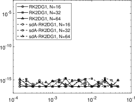
(a) (sdA-)RK2DG1, $m=1$

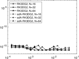
(b) (sdA-)RK3DG2, $m=1$

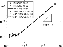
(c) (sdA-)RK4DG3, $m=1$

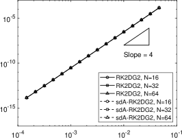
(d) (sdA-)RK2DG2, $m=1$

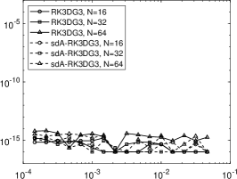
(e) (sdA-)RK3DG3, $m=1$

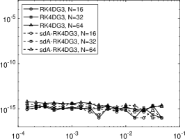
(f) (sdA-)RK4DG3, $m=2$

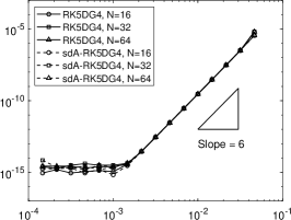
(g) (sdA-)RK5DG4, $m=1$

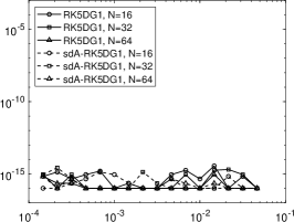
(h) (sdA-)RK5DG1, $m=1$

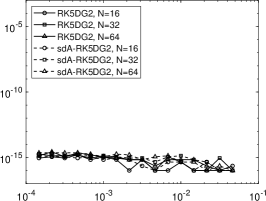
(i) (sdA-)RK5DG2, $m=2$

Figure 5.1. Stability verification for 1D RKDG and sdA-RKDG schemes. The $x$ axis is the CFL number. The $y$ axis is the value of $\delta$ defined in (5.1).

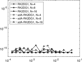
(a) (sdA-)RK2DG1, $m=1$

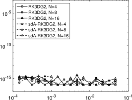
(b) (sdA-)RK3DG2, $m=1$

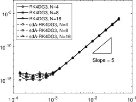
(c) (sdA-)RK4DG3, $m=1$

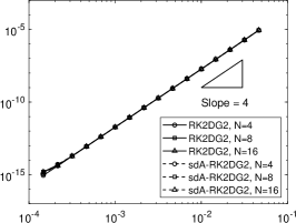
(d) (sdA-)RK2DG2, $m=1$

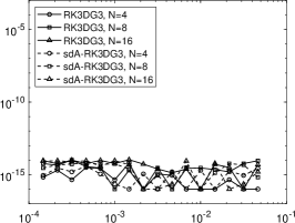
(e) (sdA-)RK3DG3, $m=1$

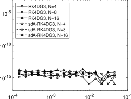
(f) (sdA-)RK4DG3, $m=2$

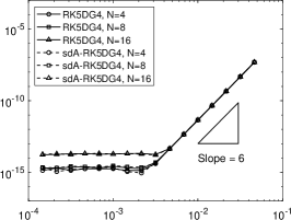
(g) (sdA-)RK5DG4, $m=1$

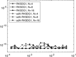
(h) (sdA-)RK5DG1, $m=1$

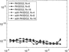
(i) (sdA-)RK5DG2, $m=2$

Figure 5.2. Stability verification for 2D RKDG and sdA-RKDG schemes. The $x$ axis is the CFL number. The $y$ axis is value of $\delta$ defined in (5.1).

5.2. Accuracy tests with smooth solutions

In this test, we consider the linear advection equation with sufficiently smooth solutions. For the 1D problem, we set $u(x,0)=\sin(2\pi x)$, and the exact solution is $u(x,t)=\sin(2\pi(x-t))$. In the 2D problem, we set $u(x,y,0)=\sin(2\pi(x+y))$, and the exact solution is $u(x,y,t)=\sin(2\pi(x+y-2t))$. The final time is set as $t^{n}=1$. We solve the problem using RK$r$DG$k$ and sdA-RK$r$DG$k$ methods with $r=k+1=2,3,4,5$. The time step size is set as $\tau=0.1/(dN)$ for $r=2,3,4$, and $\tau=0.1/(dN^{6/5})$ for $r=5$.

The $L^{2}$ errors of the numerical solutions on 1D uniform meshes, 1D randomly perturbed nonuniform meshes, and 2D uniform meshes are provided in Tables 5.2, 5.3, and 5.4, respectively. As observed, in all cases, the sdA-RKDG schemes achieve the optimal convergence rate, with numerical errors comparable to the corresponding RKDG schemes.

RKDG RK2DG1 RK3DG2 RK4DG3 RK5DG4 $N$ $L^{2}$ error Order $L^{2}$ error Order $L^{2}$ error Order $L^{2}$ error Order 20 6.90e-03 - 5.67e-04 - 3.46e-05 - 1.71e-06 - 40 1.73e-03 2.00 7.12e-05 2.99 2.17e-06 4.00 5.67e-08 4.91 80 4.37e-04 1.98 8.91e-06 3.00 1.35e-07 4.00 1.62e-09 5.13 160 1.10e-04 1.99 1.11e-06 3.00 8.46e-09 4.00 5.07e-11 5.00 320 2.77e-05 1.99 1.39e-07 3.00 5.29e-10 4.00 1.58e-12 5.00 sdA-RKDG sdA-RK2DG1 sdA-RK3DG2 sdA-RK4DG3 sdA-RK5DG4 $N$ $L^{2}$ error Order $L^{2}$ error Order $L^{2}$ error Order $L^{2}$ error Order 20 8.23e-03 - 7.67e-04 - 4.98e-05 - 2.10e-06 - 40 2.10e-03 1.97 9.62e-05 3.00 3.12e-06 4.00 7.03e-08 4.90 80 5.34e-04 1.98 1.20e-05 3.00 1.95e-07 4.00 2.12e-09 5.05 160 1.35e-04 1.99 1.51e-06 3.00 1.22e-08 4.00 6.03e-11 5.13 320 3.38e-05 1.99 1.88e-07 3.00 7.63e-10 4.00 1.85e-12 5.03

Table 5.2. Error table of the RKDG and sdA-RKDG methods for 1D linear advection equation on uniform meshes. $u(x,0)=\sin(2\pi x)$. $t^{n}=1$.

RKDG RK2DG1 RK3DG2 RK4DG3 RK5DG4 $N$ $L^{2}$ error Order $L^{2}$ error Order $L^{2}$ error Order $L^{2}$ error Order 20 7.12e-03 - 6.54e-04 - 4.16e-05 - 2.43e-06 - 40 1.84e-03 1.95 8.06e-05 3.02 2.65e-06 3.97 7.51e-08 5.02 80 4.68e-04 1.97 1.03e-05 2.97 1.70e-07 3.96 1.99e-09 5.24 160 1.16e-04 2.01 1.32e-06 2.97 1.05e-08 4.01 7.72e-11 4.69 320 2.96e-05 1.97 1.60e-07 3.04 6.55e-10 4.01 2.23e-12 5.11 sdA-RKDG sdA-RK2DG1 sdA-RK3DG2 sdA-RK4DG3 sdA-RK5DG4 $N$ $L^{2}$ error Order $L^{2}$ error Order $L^{2}$ error Order $L^{2}$ error Order 20 8.12e-03 - 7.91e-04 - 5.64e-05 - 2.97e-06 - 40 2.09e-03 1.96 1.01e-04 2.97 3.67e-06 3.94 8.72e-08 5.09 80 5.33e-04 1.97 1.28e-05 2.98 2.11e-07 4.12 2.75e-09 4.99 160 1.34e-04 1.99 1.58e-06 3.02 1.31e-08 4.01 7.92e-11 5.12 320 3.33e-05 2.01 2.01e-07 2.98 8.77e-10 3.90 2.48e-12 5.00

Table 5.3. Error table of the RKDG and sdA-RKDG methods for 1D linear advection equation on randomly perturbed nonuniform meshes. Each node is randomly perturbed by $15\%$ of the mesh size. $u(x,0)=\sin(2\pi x)$. $t^{n}=1$.

RKDG RK2DG1 RK3DG2 RK4DG3 RK5DG4 $N$ $L^{2}$ error Order $L^{2}$ error Order $L^{2}$ error Order $L^{2}$ error Order 20 2.54e-02 - 4.06e-03 - 4.36e-04 - 3.88e-05 - 40 6.98e-03 1.87 5.14e-04 2.98 2.74e-05 3.99 1.23e-06 4.98 80 1.87e-03 1.90 6.45e-05 3.00 1.72e-06 4.00 3.82e-08 5.00 160 4.86e-04 1.94 8.06e-06 3.00 1.07e-07 4.00 1.19e-09 5.00 320 1.24e-04 1.97 1.01e-06 3.00 6.72e-09 4.00 3.73e-11 5.00 sdA-RKDG sdA-RK2DG1 sdA-RK3DG2 sdA-RK4DG3 sdA-RK5DG4 $N$ $L^{2}$ error Order $L^{2}$ error Order $L^{2}$ error Order $L^{2}$ error Order 20 2.83e-02 - 4.72e-03 - 5.28e-04 - 4.37e-05 - 40 7.88e-03 1.85 5.97e-04 2.98 3.32e-05 3.99 1.37e-06 4.99 80 2.10e-03 1.91 7.48e-05 3.00 2.08e-06 4.00 4.20e-08 5.03 160 5.41e-04 1.95 9.36e-06 3.00 1.30e-07 4.00 1.30e-09 5.02 320 1.38e-04 1.98 1.17e-06 3.00 8.13e-09 4.00 4.02e-11 5.02

Table 5.4. Error table of the RKDG and sdA-RKDG methods for 2D linear advection equation on uniform meshes. $u(x,y,0)=\sin(2\pi(x+y))$. $t^{n}=1$.

5.3. Accuracy tests with solutions of limited regularity

When $r=k+1$, Theorem 4.10 indicates that the optimal $r$th-order convergence rate for RK$r$DG$k$ schemes can only be attained if $\flat\geq r+1=k+2$. To verify the sharpness of this regularity number, we consider the linear advection equation with the initial condition

$$u(x,0)=\left(\sin(2\pi x)\right)^{\flat-\frac{1}{3}}$$ (5.2)

for the 1D problem. Note that the solution is in $C^{\flat-1}(\overline{\Omega})\cap H^{\flat}(\Omega_{h})$ but not in $C^{\flat}(\overline{\Omega})\cap H^{\flat+1}(\Omega_{h})$ [46, 45]. When we set $\flat=r=k+1$, observations from Tables 5.5 and 5.6 show that both the RK$r$DG$k$ and the sdA-RK$r$DG$k$ methods exhibit suboptimal convergence for $r=k+1=2,3,4,5$. Here we have chosen a large final time to make the order degeneracy observable for $r=k+1=4,5$. Conversely, under the same settings with $\flat=r+1=k+2$, all schemes achieve optimal convergence rates. A similar test has been conducted for the 2D case with the initial condition $u(x,y,0)=\left(\sin(2\pi(x+y))\right)^{\flat-\frac{1}{3}}$, where $r=k+1=2,3$. See Table 5.7.

$\flat$ $\flat=r$ $\flat=r+1$ $\flat=r$ $\flat=r+1$ RKDG RK2DG1 RK3DG2 $N$ $L^{2}$ error Order $L^{2}$ error Order $L^{2}$ error Order $L^{2}$ error Order 80 2.25e-03 - 1.16e-03 - 5.93e-05 - 7.22e-05 - 160 7.14e-04 1.66 2.70e-04 2.10 8.24e-06 2.85 9.07e-06 2.99 320 2.30e-04 1.63 6.59e-05 2.04 1.18e-06 2.81 1.13e-06 3.00 640 7.49e-05 1.62 1.63e-05 2.02 1.75e-07 2.76 1.42e-07 3.00 1280 2.45e-05 1.61 4.84e-06 2.00 2.68e-08 2.70 1.77e-08 3.00 sdA-RKDG sdA-RK2DG1 sdA-RK3DG2 $N$ $L^{2}$ error Order $L^{2}$ error Order $L^{2}$ error Order $L^{2}$ error Order 80 2.00e-03 - 1.24e-03 - 7.36e-05 - 9.76e-05 - 160 6.35e-04 1.66 3.07e-04 2.01 9.73e-06 2.92 1.22e-05 2.99 320 2.05e-04 1.63 7.71e-05 2.00 1.30e-06 2.90 1.53e-06 3.00 640 6.66e-05 1.62 1.93e-05 2.00 1.79e-07 2.86 1.92e-07 3.00 1280 2.19e-05 1.61 4.84e-06 2.00 2.56e-08 2.81 2.40e-08 3.00

Table 5.5. Error table of the RK$r$DG$k$ and the sdA-RK$r$DG$k$ methods for 1D linear advection equation on uniform meshes. $u(x,0)=(\sin(2\pi x))^{\flat-1/3}$. $r=k+1=2,3$. $t^{n}=1$.

$\flat$ $\flat=r$ $\flat=r+1$ $\flat=r$ $\flat=r+1$ RKDG RK4DG3 RK5DG4 $N$ $L^{2}$ error Order $L^{2}$ error Order $L^{2}$ error Order $L^{2}$ error Order 20 4.47e-03 - 7.23e-03 - 3.69e-04 - 5.43e-04 - 40 2.45e-04 4.19 2.72e-04 4.73 1.10e-05 5.07 1.43e-05 5.25 80 1.75e-05 3.81 1.50e-05 4.18 3.65e-07 4.91 4.43e-07 5.01 160 1.38e-06 3.66 9.03e-07 4.05 1.26e-08 4.86 1.39e-08 5.00 320 1.17e-07 3.56 5.57e-08 4.02 4.47e-10 4.82 4.33e-10 5.00 sdA-RKDG sdA-RK4DG3 sdA-RK5DG4 $N$ $L^{2}$ error Order $L^{2}$ error Order $L^{2}$ error Order $L^{2}$ error Order 20 3.55e-03 - 5.68e-03 - 3.97e-04 - 5.94e-04 - 40 2.19e-04 4.02 2.80e-04 4.34 1.24e-05 5.00 1.76e-05 5.08 80 1.58e-05 3.79 1.62e-05 4.11 3.97e-07 4.96 5.37e-07 5.04 160 1.27e-06 3.64 9.80e-07 4.05 1.31e-08 4.92 1.65e-08 5.03 320 1.10e-07 3.52 6.04e-08 4.02 4.49e-10 4.87 5.07e-10 5.02

Table 5.6. Error table of the RK$r$DG$k$ and the sdA-RK$r$DG$k$ methods for 1D linear advection equation on uniform meshes. $u(x,0)=(\sin(2\pi x))^{\flat-1/3}$. $r=k+1=4,5$. $t^{n}=500$.

$\flat$ $\flat=r$ $\flat=r+1$ $\flat=r$ $\flat=r+1$ RKDG RK2DG1 RK3DG2 $N$ $L^{2}$ error Order $L^{2}$ error Order $L^{2}$ error Order $L^{2}$ error Order 20 7.28e-02 - 9.18e-02 - 1.79e-02 - 2.44e-02 - 40 2.20e-02 1.73 2.12e-02 2.11 2.76e-03 2.70 3.88e-03 2.65 80 6.52e-03 1.75 4.55e-03 2.22 3.88e-04 2.83 5.17e-04 2.91 160 2.06e-03 1.66 1.07e-03 2.08 5.34e-05 2.86 6.55e-05 2.98 320 6.66e-04 1.63 2.72e-04 1.98 7.41e-06 2.85 8.21e-06 3.00 sdA-RKDG sdA-RK2DG1 sdA-RK3DG2 $N$ $L^{2}$ error Order $L^{2}$ error Order $L^{2}$ error Order $L^{2}$ error Order 20 6.89e-02 - 8.15e-02 - 2.05e-02 - 2.88e-02 - 40 2.03e-02 1.77 1.98e-02 2.04 3.15e-03 2.70 4.54e-03 2.67 80 6.09e-03 1.74 4.56e-03 2.12 4.36e-04 2.85 6.00e-04 2.92 160 1.93e-03 1.66 1.15e-03 1.99 5.88e-05 2.89 7.60e-05 2.98 320 6.22e-04 1.63 2.97e-04 1.95 7.94e-06 2.89 9.53e-06 3.00

Table 5.7. Error table of the RK$r$DG$k$ and the sdA-RK$r$DG$k$ methods for 2D linear advection equation on uniform meshes. $u(x,y,0)=(\sin(2\pi(x+y)))^{\flat-1/3}$. $r=k+1=2,3$. $t^{n}=1$.

5.4. Tests of matrix sparsity

The efficiency of implementing RKDG and sdA-RKDG schemes can be assessed by counting the total number of nonzero entries in the matrices in the final matrix equation. Below, we consider the 2D problem with $s=r=k+1$. The DG spatial operator is implemented under the orthonormal Legendre basis. We consider four implementations: Horner’s implementation of sdA-RKDG schemes, Horner’s implementation of RKDG schemes, implementation of sdA-RKDG schemes by assembling $\widetilde{R}_{h}$, and implementation of RKDG schemes by assembling $R_{h}$. In Table 5.8, we summarize the number of nonzero matrix entries per mesh cell in a single time step (excluding identity matrices). The results indicate that for 2D problems, sdA-RKDG schemes may offer greater efficiency compared to standard RKDG schemes. For $2\leq s=r=k+1\leq 9$, the computational cost of sdA-RKDG schemes ranges from $70.6\%$ to $86.1\%$ compared to that of RKDG schemes.

$s$ $\mathcal{N}_{\widetilde{R}_{h}-\mathrm{H}}$ $\mathcal{N}_{R_{h}-\mathrm{H}}$ Ratio Prediction $\mathcal{N}_{\widetilde{R}_{h}}$ $\mathcal{N}_{R_{h}}$ $2$ 24 34 70.6% 66.7% 42 46 $3$ 108 150 72.0% 66.7% 306 312 $4$ 332 440 75.5% 70.0% 1354 1360 $5$ 805 1025 78.5% 73.3% 4379 4385 $6$ 1668 2058 81.0% 76.2% 8554 8561 $7$ 3094 3724 83.1% 78.6% 15170 15176 $8$ 5288 6240 84.7% 80.6% 25026 25032 $9$ 8487 9855 86.1% 82.2% 39039 39045

Table 5.8. Nonzero matrix entries per mesh cell in the implementation of the RK$r$DG$k$ and the sdA-RK$r$DG$k$ schemes with $s$ stages, where $s=r=k+1$. Here $\mathcal{N}(A)$ denotes the number of nonzero entries in the matrix $A$, $\mathcal{N}_{\widetilde{R}_{h}-\mathrm{H}}=(\mathcal{N}(L_{h})+(s-1)\mathcal{N}(\widetilde{L}_{h}))/N^{2}$ corresponds to the Horner’s implementation of the sdA-RKDG schemes, and $\mathcal{N}_{R_{h}-\mathrm{H}}=s\mathcal{N}(L_{h})/N^{2}$ corresponds to the Horner’s implementation of the RKDG schemes. The “Ratio” is $\mathcal{N}_{\widetilde{R}_{h}-\mathrm{H}}:\mathcal{N}_{R_{h}-\mathrm{H}}$, and the “Prediction” is $sk+d:s(k+d)=s(s-1)+2:s(s+1)$ as explained in Remark 2.2. $\mathcal{N}_{\widetilde{R}_{h}}$ corresponds to the implementation of the sdA-RKDG schemes by assembling $\widetilde{R}_{h}$, and $\mathcal{N}_{R_{h}}$ corresponds to the implementation of the sdA-RKDG schemes by assembling $R_{h}$.

6. Proofs of technical lemmas

6.1. Proof of Lemma 3.5

We will consider the 1D and 2D cases separately.

1D case. Using the self-adjoint property of $\Pi_{\perp}$, the definition of $L_{h}$, and the integration by parts, one can get

$$\left(\Pi_{\perp}L_{h}w_{h},v_{h}\right)= \left(L_{h}w_{h},\Pi_{\perp}v_{h}\right)$$ (6.1)

$$= \beta\left(w_{h},(\Pi_{\perp}v_{h})_{x}\right)-\beta\sum_{i=1}^{N}\left(({w}_{h}^{-}(\Pi_{\perp}v_{h})^{-})_{i+\frac{1}{2}}-({w}_{h}^{-}(\Pi_{\perp}v_{h})^{+})_{i-\frac{1}{2}}\right)$$

$$= -\beta\left((w_{h})_{x},\Pi_{\perp}v_{h}\right)-\beta\sum_{i=1}^{N}([w_{h}](\Pi_{\perp}v_{h})^{+})_{i-\frac{1}{2}}.$$

Note that $(w_{h})_{x}\in V_{h}^{k-1}$ and $\Pi_{\perp}v_{h}\perp V_{h}^{k-1}$. Thus, $\left((w_{h})_{x},\Pi_{\perp}v_{h}\right)=0$ and

$$\left(\Pi_{\perp}L_{h}w_{h},v_{h}\right)=-\beta\sum_{i=1}^{N}([w_{h}](\Pi_{\perp}v_{h})^{+})_{i-\frac{1}{2}}\leq C\left\llbracket w_{h}\right\rrbracket\left\|\Pi_{\perp}v_{h}\right\|_{\Gamma}.$$ (6.2)

Here we have used the Cauchy–Schwarz inequality. With the inverse estimate (2.20), we get

$$\left\|\Pi_{\perp}v_{h}\right\|_{\Gamma}\leq Ch^{-1/2}\left\|\Pi_{\perp}v_{h}\right\|\leq Ch^{-1/2}\left\|v_{h}\right\|.$$ (6.3)

Substituting (6.3) into (6.2) completes the proof of (3.7a) in the 1D case.

For the proof of (3.7b), note we have [51, 36]

$$\left(L_{h}^{\top}w_{h},v_{h}\right)=-\beta\left(w_{h},(v_{h})_{x}\right)+\beta\sum_{i=1}^{N}\left((w_{h}^{+}v_{h}^{-})_{i+\frac{1}{2}}-(w_{h}^{+}v_{h}^{+})_{i-\frac{1}{2}}\right).$$ (6.4)

Comparing (6.4) to (2.3), $L_{h}^{\top}$ can be defined by replacing the numerical flux $w_{h}^{-}$ in (2.3) by $w_{h}^{+}$ and changing the sign of each term. One can take advantage of this similar structure to prove (3.7b) by following similar lines as those in the proof of (3.7a).

$$\left(\Pi_{\perp}L_{h}^{\top}w_{h},v_{h}\right)=\left(L_{h}^{\top}w_{h},\Pi_{\perp}v_{h}\right)$$ (6.5)

$$= -\beta\left(w_{h},(\Pi_{\perp}v_{h})_{x}\right)+\beta\sum_{i=1}^{N}\left(({w}_{h}^{+}(\Pi_{\perp}v_{h})^{-})_{i+\frac{1}{2}}-({w}_{h}^{+}(\Pi_{\perp}v_{h})^{+})_{i-\frac{1}{2}}\right)$$

$$= \beta\left((w_{h})_{x},\Pi_{\perp}v_{h}\right)+\beta\sum_{i=1}^{N}([w_{h}](\Pi_{\perp}v_{h})^{-})_{i+\frac{1}{2}}=\beta\sum_{i=1}^{N}([w_{h}](\Pi_{\perp}v_{h})^{-})_{i+\frac{1}{2}}$$

$$\leq C\left\llbracket w_{h}\right\rrbracket\left\|\Pi_{\perp}v_{h}\right\|_{\Gamma}\leq Ch^{-\frac{1}{2}}\left\llbracket w_{h}\right\rrbracket\left\|\Pi_{\perp}v_{h}\right\|\leq Ch^{-\frac{1}{2}}\left\llbracket w_{h}\right\rrbracket\left\|v_{h}\right\|.$$

2D case. Similar to the 1D case, we use the self-adjoint property of $\Pi_{\perp}$, the definition of $L_{h}$, and the integration by parts. It yields

$$\left(\Pi_{\perp}L_{h}w_{h},v_{h}\right)=\left(L_{h}w_{h},\Pi_{\perp}v_{h}\right)$$ (6.6)

$$= \left(w_{h},\beta^{x}(\Pi_{\perp}v_{h})_{x}+\beta^{y}(\Pi_{\perp}v_{h})_{y}\right)$$

$$-\sum_{i=1}^{N_{x}}\sum_{j=1}^{N_{y}}\int_{x_{i-\frac{1}{2}}}^{x_{i+\frac{1}{2}}}\beta^{y}\left(w_{h}\left(x,y_{j+\frac{1}{2}}^{-}\right)(\Pi_{\perp}v_{h})\left(x,y_{j+\frac{1}{2}}^{-}\right)-w_{h}\left(x,y_{j-\frac{1}{2}}^{-}\right)(\Pi_{\perp}v_{h})\left(x,y_{j-\frac{1}{2}}^{+}\right)\right)\mathrm{d}x$$

$$-\sum_{i=1}^{N_{x}}\sum_{j=1}^{N_{y}}\int_{y_{j-\frac{1}{2}}}^{y_{j+\frac{1}{2}}}\beta^{x}\left(w_{h}\left(x_{i+\frac{1}{2}}^{-},y\right)(\Pi_{\perp}v_{h})\left(x_{i+\frac{1}{2}}^{-},y\right)-w_{h}\left(x_{i-\frac{1}{2}}^{-},y\right)(\Pi_{\perp}v_{h})\left(x_{i-\frac{1}{2}}^{+},y\right)\right)\mathrm{d}y$$

$$= -\left(\beta^{x}(w_{h})_{x}+\beta^{y}(w_{h})_{y},\Pi_{\perp}v_{h}\right)-\sum_{i=1}^{N_{x}}\sum_{j=1}^{N_{y}}\int_{x_{i-\frac{1}{2}}}^{x_{i+\frac{1}{2}}}\beta^{y}[w_{h}]_{i,j-\frac{1}{2}}(\Pi_{\perp}v_{h})\left(x,y_{j-\frac{1}{2}}^{+}\right)\mathrm{d}x$$

$$-\sum_{i=1}^{N_{x}}\sum_{j=1}^{N_{y}}\int_{y_{j-\frac{1}{2}}}^{y_{j+\frac{1}{2}}}\beta^{x}[w_{h}]_{i-\frac{1}{2},j}(\Pi_{\perp}v_{h})\left(x_{i-\frac{1}{2}}^{+},y\right)\mathrm{d}y.$$

Note that the first term is $0$ since $(\beta^{x}\partial_{x}+\beta^{y}\partial_{y})w_{h}\in V_{h}^{k-1}$ and $\Pi_{\perp}v_{h}\perp V_{h}^{k-1}$. As we have done for the 1D case, we can then prove the lemma by applying the Cauchy–Schwarz inequality, the inverse estimate, and the fact $\left\|\Pi_{\perp}v_{h}\right\|\leq\left\|v_{h}\right\|$. The 2D case of (3.7b) can be proved similarly by rewriting $L_{h}^{\top}$ in a similar form as (6.4). Details are omitted.

6.2. Proof of Lemma 3.14

To prove Lemma 3.14, we need a few preparatory lemmas.

Lemma 6.1 (Discrete integration by parts).

$$\left(L_{h}^{i}w_{h},v_{h}\right)=\sum_{j=0}^{i-1}(-1)^{j+1}\left[L_{h}^{i-j-1}w_{h},L_{h}^{j}v_{h}\right]+(-1)^{i}\left(w_{h},L_{h}^{i}v_{h}\right).$$ (6.7)

Proof.

Recall Proposition 2.1. The lemma can be proved by inductively applying $\left(L_{h}w_{h},v_{h}\right)=-\left[w_{h},v_{h}\right]-\left(w_{h},L_{h}v_{h}\right)$. Details are omitted. ∎

Lemma 6.2.

$$\left\llbracket L_{h}^{i}\Pi_{\perp}L_{h}w_{h}\right\rrbracket\leq Ch^{-i-1}\left\llbracket w_{h}\right\rrbracket\qquad\forall i\geq 0.$$ (6.8)

Proof.

With the inverse estimate $\left\llbracket v_{h}\right\rrbracket\leq Ch^{-\frac{1}{2}}\left\|v_{h}\right\|$ and the property $\left\|L_{h}\right\|\leq Ch^{-1}$, we have

$$\left\llbracket L_{h}^{i}\Pi_{\perp}L_{h}w_{h}\right\rrbracket\leq Ch^{-\frac{1}{2}}\left\|L_{h}^{i}\Pi_{\perp}L_{h}w_{h}\right\|\leq Ch^{-\frac{1}{2}}\left\|L_{h}\right\|^{i}\left\|\Pi_{\perp}L_{h}w_{h}\right\|\leq Ch^{-i-\frac{1}{2}}\left\|\Pi_{\perp}L_{h}w_{h}\right\|.$$ (6.9)

Note from (3.7a), we have $\left\|\Pi_{\perp}L_{h}w_{h}\right\|\leq Ch^{-1/2}\left\llbracket w_{h}\right\rrbracket$. Applying this estimate to (6.9) completes the proof of (6.8). ∎

Now we prove Lemma 3.14.

Proof of Lemma 3.14.

We define $z_{h}$ such that $L_{h}^{\underline{i}}w_{h}=L_{h}^{i_{1}}\Pi_{\perp}L_{h}z_{h}$. In other words,

$$z_{h}= L_{h}^{i_{2}-1}\Pi_{\perp}L_{h}^{i_{3}}\cdots\Pi_{\perp}L_{h}^{i_{|\underline{i}|}}w_{h}$$ (6.10)

$$= \left(L_{h}^{i_{2}-1}\Pi_{\perp}L_{h}\right)\left(L_{h}^{i_{3}-1}\Pi_{\perp}L_{h}\right)\cdots\left(L_{h}^{i_{|\underline{i}|-1}-1}\Pi_{\perp}L_{h}\right)L_{h}^{i_{|\underline{i}|}-1}w_{h}.$$

First, with Lemma 6.1, the triangle inequality, and the Cauchy–Schwarz inequality, we have

$$\left|\left(L_{h}^{\underline{i}}w_{h},v_{h}\right)\right|$$ (6.11)

$$= \left|\left(L_{h}^{i_{1}-1}(L_{h}\Pi_{\perp}L_{h}z_{h}),v_{h}\right)\right|$$

$$= \left|\sum_{j=0}^{i_{1}-2}(-1)^{j+1}\left[L_{h}^{i_{1}-j-1}\Pi_{\perp}L_{h}z_{h},L_{h}^{j}v_{h}\right]+(-1)^{i_{1}-1}\left(L_{h}\Pi_{\perp}L_{h}z_{h},L_{h}^{i_{1}-1}v_{h}\right)\right|$$

$$\leq \sum_{j=0}^{i_{1}-2}\left\llbracket L_{h}^{i_{1}-j-1}\Pi_{\perp}L_{h}z_{h}\right\rrbracket\left\llbracket L_{h}^{j}v_{h}\right\rrbracket+|\left(L_{h}\Pi_{\perp}L_{h}z_{h},L_{h}^{i_{1}-1}v_{h}\right)|.$$

Then we apply Lemmas 6.2 and 3.6 to get

$$\left|\left(L_{h}^{\underline{i}}w_{h},v_{h}\right)\right|\leq C\sum_{j=0}^{i_{1}-2}h^{-(i_{1}-j)}\left\llbracket z_{h}\right\rrbracket\left\llbracket L_{h}^{j}v_{h}\right\rrbracket+Ch^{-1}\left\llbracket z_{h}\right\rrbracket\left\llbracket L_{h}^{i_{1}-1}v_{h}\right\rrbracket$$ (6.12)

$$= C\sum_{j=0}^{i_{1}-1}h^{-(i_{1}-j)}\left\llbracket z_{h}\right\rrbracket\left\llbracket L_{h}^{j}v_{h}\right\rrbracket.$$

Next, recall the definition of $z_{h}$ in (6.10) and apply Lemma 6.2 for $[\underline{i}]-2$ times. We have

$$\left\llbracket z_{h}\right\rrbracket\leq Ch^{-i_{2}-i_{3}-\cdots-i_{[\underline{i}]-1}}\left\llbracket L_{h}^{i_{[\underline{i}]}-1}w_{h}\right\rrbracket\leq Ch^{-|\underline{i}|+i_{1}+i_{[\underline{i}]}}\left\llbracket L_{h}^{i_{[\underline{i}]}-1}w_{h}\right\rrbracket.$$ (6.13)

Finally, one can complete the proof of Lemma 3.14 by substituting (6.13) into (6.12). ∎

6.3. Proof of Lemma 4.2

First, the well-definedness of $\Pi_{G}$ was prove in [28, Lemma 2.4]. Then, (4.5) follows from the standard approximation theorem [4]. See also [28, (2.19)]. Next, for (4.6), the case $\ell=k+2$ is a Cauchy–Schwarz version of [28, (2.30)]. Finally, for the case $1\leq\ell\leq k+1$, one can follow a similar argument as the standard suboptimal error estimate of the DG scheme. To be more specific, with $\eta=\Pi_{G}w-w$, we have

$$\left((\Pi L-L_{h}\Pi_{G})w,v_{h}\right)=\left(Lw,v_{h}\right)-\left(L_{h}\Pi_{G}w,v_{h}\right)=\left(\eta,\beta^{x}(v_{h})_{x}+\beta^{y}(v_{h})_{y}\right)$$ (6.14)

$$-\sum_{i=1}^{N_{x}}\sum_{j=1}^{N_{y}}\int_{x_{i-\frac{1}{2}}}^{x_{i+\frac{1}{2}}}\beta^{y}\left(\eta\left(x,y_{j+\frac{1}{2}}^{-}\right)v_{h}\left(x,y_{j+\frac{1}{2}}^{-}\right)-\eta\left(x,y_{j-\frac{1}{2}}^{-}\right)v_{h}\left(x,y_{j-\frac{1}{2}}^{+}\right)\right)\mathrm{d}x$$

$$-\sum_{i=1}^{N_{x}}\sum_{j=1}^{N_{y}}\int_{y_{j-\frac{1}{2}}}^{y_{j+\frac{1}{2}}}\beta^{x}\left(\eta\left(x_{i+\frac{1}{2}}^{-},y\right)v_{h}\left(x_{i+\frac{1}{2}}^{-},y\right)-\eta\left(x_{i-\frac{1}{2}}^{-},y\right)v_{h}\left(x_{i-\frac{1}{2}}^{+},y\right)\right)\mathrm{d}y$$

$$\leq C\left\|\eta\right\|\left\|v_{h}\right\|_{H^{1}}+C\left\|\eta\right\|_{\Gamma}\left\llbracket v_{h}\right\rrbracket\leq C\left(h^{-1}\left\|\eta\right\|+h^{-\frac{1}{2}}\left\|\eta\right\|_{\Gamma}\right)\left\|v_{h}\right\|.$$

Note with the approximation property of $\eta$ and the trace inequality, it can be seen that $\left\|\eta\right\|\leq C\left\|w\right\|_{H^{\min(\ell,\flat)}}h^{\min(\ell,\flat)}$ and $\left\|\eta\right\|_{\Gamma}\leq C\left\|\eta\right\|^{1/2}\left\|\eta\right\|_{H^{1}}^{1/2}\leq C\left\|w\right\|_{H^{\min(\ell,\flat)}}h^{\min(\ell,\flat)-1/2}$. Substituting these estimates into (6.14) completes the proof of (4.6) for the case $1\leq\ell\leq k+1$.

6.4. Proof of Lemma 4.5

1. (4.10) follows from (4.7) and the standard approximation theory [4].

2. To prove (4.11) for $\overline{\Pi}=\Pi,\Pi_{G}$, we consider (4.10) with $w=L\tilde{w}$, $\ell=\tilde{\ell}-1$, and $\flat=\tilde{\flat}-1$. Note that, in the case $\tilde{w}\in H^{\tilde{\flat}}(\Omega_{h})$, $1\leq\tilde{\ell}\leq k+2$ and $\tilde{\flat}\geq 2$, we have $w\in H^{\flat}(\Omega_{h})$, $0\leq\ell\leq k+1$ and $\flat\geq 1$. Hence (4.10) can be applied, which gives

$$\left\|(I-\overline{\Pi})L\tilde{w}\right\|\leq C\left\|L\tilde{w}\right\|_{H^{\min(\tilde{\ell}-1,\tilde{\flat}-1)}}h^{\min(\tilde{\ell}-1,\tilde{\flat}-1)}\leq C\left\|\tilde{w}\right\|_{H^{\min(\tilde{\ell},\tilde{\flat})}}h^{\min(\tilde{\ell},\tilde{\flat})-1}.$$ (6.15)

We can complete the proof of (4.11) after removing the tilde symbol. The proof for $\overline{\Pi}=\Pi_{k-1}$ is similar.

3. Similarly, for (4.12), we consider (4.8) with $w=L^{i}\tilde{w}$, $\ell=\tilde{\ell}-i$, $\flat=\tilde{\flat}-i$, and $v_{h}=\left(\Pi L-L_{h}\Pi_{G}\right)L^{i}\tilde{w}^{n}$. Note that, in the case $\tilde{w}\in C^{\tilde{\flat}-1}(\overline{\Omega})\cap H^{\tilde{\flat}}(\Omega_{h})$, $1\leq\tilde{\ell}\leq k+2$, and $0\leq i\leq\min(\tilde{\ell},\tilde{\flat})-1$, we have $w\in C(\overline{\Omega})\cap H^{\flat}(\Omega_{h})$ and $1\leq\ell\leq k+2$. Thus, (4.8) holds and

$$\left\|\left(\Pi L-L_{h}\Pi_{G}\right)L^{i}\tilde{w}\right\|\leq C_{d}\left\|L^{i}\tilde{w}\right\|_{H^{\min(\tilde{\ell}-i,\tilde{\flat}-i)}}h^{\min(\tilde{\ell}-i,\tilde{\flat}-i)-1}$$ (6.16)

$$\leq C_{d}\left\|\tilde{w}\right\|_{H^{\min(\tilde{\ell},\tilde{\flat})}}h^{\min(\tilde{\ell},\tilde{\flat})-i-1}.$$

The proof is completed after removing the tilde symbol.

4. Since $\widetilde{L}_{h}=(I-\Pi_{\perp})L_{h}$, adding and subtracting terms gives

$$(\Pi L-\widetilde{L}_{h}\Pi_{G})w= \left(\Pi L-L_{h}\Pi_{G}\right)w+\Pi_{\perp}L_{h}\Pi_{G}w$$ (6.17)

$$= \left(\Pi L-L_{h}\Pi_{G}\right)w+\Pi_{\perp}\left(L_{h}\Pi_{G}-\Pi L\right)w+\Pi_{\perp}\Pi Lw$$

$$= (I-\Pi_{\perp})\left(\Pi L-L_{h}\Pi_{G}\right)w-\Pi_{\perp}(I-\Pi)Lw+\Pi_{\perp}Lw.$$

For $1\leq\ell\leq k+1$, with (4.11) in Lemma 4.5, it can be seen that

$$\left\|\Pi_{\perp}(I-\Pi)Lw\right\|\leq\left\|(I-\Pi)Lw\right\|\leq C\left\|w\right\|_{H^{\min(\ell,\flat)}}h^{\min(\ell,\flat)-1},$$ (6.18)

$$\left\|\Pi_{\perp}Lw\right\|=\left\|(I-\Pi_{k-1})Lw\right\|\leq C\left\|w\right\|_{H^{\min(\ell,\flat)}}h^{\min(\ell,\flat)-1}.$$ (6.19)

With (4.12) in Lemma 4.5, we have

$$\left\|(I-\Pi_{\perp})\left(\Pi L-L_{h}\Pi_{G}\right)w\right\|\leq\left\|\left(\Pi L-L_{h}\Pi_{G}\right)w\right\|\leq C_{d}\left\|w\right\|_{H^{\min(\ell,\flat)}}h^{\min(\ell,\flat)-1}.$$ (6.20)

Applying the triangle inequality to (6.17), and then substituting in the estimates above, we obtain (4.13).

6.5. Proof of Lemma 4.7

Lemma 6.3 (Invertibility of $I+\tau\widetilde{L}_{h}/2$).

$(I+\tau\widetilde{L}_{h}/2)^{-1}$ is well-defined when $\lambda\ll 1$. Moreover, $\left\|(I+\tau\widetilde{L}_{h}/2)^{-1}w_{h}\right\|\leq C\left\|w_{h}\right\|$.

Proof.

Consider

$$\left(I+\frac{\tau}{2}\widetilde{L}_{h}\right)v_{h}=w_{h}.$$ (6.21)

We apply the triangle inequality to get

$$\left\|v_{h}\right\|-\frac{\tau}{2}\left\|\widetilde{L}_{h}\right\|\left\|v_{h}\right\|\leq\left\|w_{h}\right\|.$$ (6.22)

Recall that $\tau\left\|\widetilde{L}_{h}\right\|\leq C\lambda$. When $\lambda\ll 1$, we have $1-\tau\left\|\widetilde{L}_{h}\right\|/2\geq 1-C\lambda/2>0$. Hence

$$\left\|v_{h}\right\|\leq\left(1-\frac{\tau}{2}\left\|\widetilde{L}_{h}\right\|\right)^{-1}\left\|w_{h}\right\|\leq\left(1-\frac{C\lambda}{2}\right)^{-1}\left\|w_{h}\right\|\leq C\left\|w_{h}\right\|.$$ (6.23)

When $w_{h}=0$, (6.23) forces $\left\|v_{h}\right\|=0$, and thus $v_{h}=0$. Therefore $I+\tau\widetilde{L}_{h}/2$ is an injection. Note that $I+\tau\widetilde{L}_{h}/2:V_{h}^{k}\to V_{h}^{k}$ is an operator on a finite-dimensional space. $I+\tau\widetilde{L}_{h}/2$ is an injection implies that $I+\tau\widetilde{L}_{h}/2$ is invertible. By rewriting $v_{h}=(I+\tau\widetilde{L}_{h}/2)^{-1}w_{h}$ in (6.23), we obtain the desired estimate. ∎

Lemma 6.4 (Commutation error of $\widetilde{L}_{h}$).

If $w\in C^{\flat-1}(\overline{\Omega})\cap H^{\flat}(\Omega_{h})$ and $\flat\geq 2$, then

$$\left\|(\Pi_{G}L-\widetilde{L}_{h}\Pi_{G})w\right\|\leq C\left\|w\right\|_{H^{\min(\ell,\flat)}}h^{\min(\ell,\flat)-1}\qquad 1\leq\ell\leq k+1.$$ (6.24)

Proof.

By triangle inequality, we have

$$\left\|(\Pi_{G}L-\widetilde{L}_{h}\Pi_{G})w\right\|\leq\left\|(\Pi L-\widetilde{L}_{h}\Pi_{G})w\right\|+\left\|(I-\Pi)Lw\right\|+\left\|(I-\Pi_{G})Lw\right\|$$ (6.25)

Since $w\in C^{\flat-1}(\overline{\Omega})\cap H^{\flat}(\Omega_{h})$ and $\flat\geq 2$, the regularity assumptions in both (4.13) and (4.11) of Lemma 4.5 hold. Applying these estimates to (6.25) would complete the proof of Lemma 6.4. ∎

Now we prove Lemma 4.7.

Proof of Lemma 4.7.

Since for $w\in C^{\flat-1}(\overline{\Omega})\cap H^{\flat}(\Omega_{h})$ with $\flat\geq 2$, we have $w+\tau Lw/2\in H^{1}(\Omega_{h})$. Thus $\Pi_{G}(w+\tau Lw/2)$ is well-defined. By Lemma 6.3, $\Pi_{\star}w=(I+\tau\widetilde{L}_{h}/2)^{-1}\Pi_{G}(w+\tau Lw/2)$ is also well-defined.

To prove the approximation estimate (4.7), note that

$$\left(\Pi_{\star}-\Pi_{G}\right)w= \left(I+\frac{\tau}{2}\widetilde{L}_{h}\right)^{-1}\Pi_{G}\left(I+\frac{\tau}{2}L\right)w-\Pi_{G}w$$ (6.26)

$$= \left(I+\frac{\tau}{2}\widetilde{L}_{h}\right)^{-1}\Pi_{G}\left(I+\frac{\tau}{2}L\right)w-\left(I+\frac{\tau}{2}\widetilde{L}_{h}\right)^{-1}\left(\Pi_{G}w+\frac{\tau}{2}\widetilde{L}_{h}\Pi_{G}w\right)$$

$$= \frac{\tau}{2}\left(I+\frac{\tau}{2}\widetilde{L}_{h}\right)^{-1}\left(\Pi_{G}L-\widetilde{L}_{h}\Pi_{G}\right)w.$$

Applying Lemmas 6.3 and 6.4, for all $1\leq\ell\leq k+1$, one can get

$$\left\|(\Pi_{\star}-\Pi_{G})w\right\|\leq C\tau\left\|(\Pi_{G}L-\widetilde{L}_{h}\Pi_{G})w\right\|\leq C\tau\left\|w\right\|_{H^{\min(\ell,\flat)}}h^{\min(\ell,\flat)-1}$$ (6.27)

$$\leq C\left\|w\right\|_{H^{\min(\ell,\flat)}}h^{\min(\ell,\flat)}.$$

Using the triangle inequality and (4.10), we have

$$\left\|\left(I-\Pi_{\star}\right)w\right\|\leq\left\|\left(I-\Pi_{G}\right)w\right\|+\left\|\left(\Pi_{G}-\Pi_{\star}\right)w\right\|\leq C\left\|w\right\|_{H^{\min(\ell,\flat)}}h^{\min(\ell,\flat)}.$$ (6.28)

∎

6.6. Proof of Lemma 4.11

Lemma 6.5 (Generalization of Lemma 6.3).

Let $\alpha_{i}=(i!)^{-1}$ for $i=0,1,\cdots,r$. The operator inversion $\left(\sum_{i=1}^{s}\alpha_{i}(\tau\widetilde{L}_{h})^{i-1}\right)^{-1}$ is well-defined if $\lambda\ll 1$. Moreover,

$$\left\|\left(\sum_{i=1}^{s}\alpha_{i}(\tau\widetilde{L}_{h})^{i-1}\right)^{-1}w_{h}\right\|\leq C\left\|w_{h}\right\|.$$ (6.29)

Proof.

Consider $\left(\sum_{i=1}^{s}\alpha_{i}(\tau\widetilde{L}_{h})^{i-1}\right)v_{h}=w_{h}$. Note that $\sum_{i=1}^{s}\alpha_{i}(\tau\widetilde{L}_{h})^{i-1}=I+\sum_{i=2}^{s}\alpha_{i}(\tau\widetilde{L}_{h})^{i-1}$. Then by the triangle inequality, we have

$$\left(1-\sum_{i=2}^{s}|\alpha_{i}|\left(\tau\left\|\widetilde{L}_{h}\right\|\right)^{i-1}\right)\left\|v_{h}\right\|\leq\left\|w_{h}\right\|.$$ (6.30)

Recall that $\tau\left\|\widetilde{L}_{h}\right\|\leq C\lambda$. By taking $\lambda\ll 1$, we can make $1-\sum_{i=2}^{s}|\alpha_{i}|(\tau\left\|\widetilde{L}_{h}\right\|)^{i-1}>0$ and hence $\left\|v_{h}\right\|\leq C\left\|w_{h}\right\|$. As a result, $w_{h}=0$ implies $v_{h}=0$. Therefore, $\sum_{i=1}^{s}\alpha_{i}(\tau\widetilde{L}_{h})^{i-1}$ is an injection on a finite-dimensional space, and hence invertible. The norm estimate also follows from (6.30) by taking $v_{h}=\left(\sum_{i=1}^{s}\alpha_{i}(\tau\widetilde{L}_{h})^{i-1}\right)^{-1}w_{h}$. ∎

Lemma 6.6 (Generalization of Lemma 6.4).

If $w\in C^{\flat-1}(\overline{\Omega})\cap H^{\flat}(\Omega_{h})$ and $\flat\geq 2$, then

$$\left\|(\Pi_{G}L^{i}-\widetilde{L}_{h}^{i}\Pi_{G})w\right\|\leq C\left\|w\right\|_{H^{\min(\ell,\flat)}}h^{\min(\ell,\flat)-i}\qquad\forall 1\leq\ell\leq k+1,$$ (6.31)

where $0\leq i\leq\min(\ell,\flat-1)$.

Proof.

We prove by induction with respect to $i$. The case $i=0$ is trivial, and the case $i=1$ is proved in Lemma 6.4. Now we assume (6.31) holds for $i-1$, and we prove the inequality holds for $i$ with $i\geq 2$. Indeed,

$$(\Pi_{G}L^{i}-\widetilde{L}_{h}^{i}\Pi_{G})w=(\Pi_{G}L^{i-1}-\widetilde{L}_{h}^{i-1}\Pi_{G})Lw+\widetilde{L}_{h}^{i-1}(\Pi_{G}Lw-\widetilde{L}_{h}\Pi_{G}w).$$ (6.32)

Noting that $2\leq i\leq\flat-1$, we have $Lw\in C^{\flat-2}(\overline{\Omega})\cap H^{\flat-1}(\Omega_{h})\subset C^{i-1}(\overline{\Omega})\cap H^{i}(\Omega_{h})\subset C^{1}(\overline{\Omega})\cap H^{2}(\Omega_{h})$. Using the induction hypothesis with $\ell$ replaced by $\ell-1$, we have

$$\left\|(\Pi_{G}L^{i-1}-\widetilde{L}_{h}^{i-1}\Pi_{G})Lw\right\|\leq C\left\|Lw\right\|_{H^{\min(\ell-1,\flat-1)}}h^{\min(\ell-1,\flat-1)-(i-1)}$$ (6.33)

$$\leq C\left\|w\right\|_{H^{\min(\ell,\flat)}}h^{\min(\ell,\flat)-i}.$$

With the fact $\left\|\widetilde{L}_{h}\right\|\leq\left\|L_{h}\right\|\leq Ch^{-1}$ and Lemma 6.4, one can get

$$\left\|\widetilde{L}_{h}^{i-1}(\Pi_{G}Lw-\widetilde{L}_{h}\Pi_{G}w)\right\|\leq Ch^{-(i-1)}\left\|(\Pi_{G}L-\widetilde{L}_{h}\Pi_{G})w\right\|$$ (6.34)

$$\leq C\left\|w\right\|_{H^{\min(\ell,\flat)}}h^{\min(\ell,\flat)-i}.$$

Finally, by applying the triangle inequality to (6.32), and invoking (6.33) and (6.34), we prove (6.31) for $i$. By induction, (6.31) holds for all $0\leq i\leq\min(\ell,\flat-1)$. ∎

Now we prove the approximation estimate of $\Pi_{\star}$.

Proof of Lemma 4.11.

$$\Pi_{\star}w-\Pi_{G}w$$ (6.35)

$$= \left(\sum_{i=1}^{s}\alpha_{i}(\tau\widetilde{L}_{h})^{i-1}\right)^{-1}\left(\Pi_{G}\left(\sum_{i=1}^{q}(i!)^{-1}(\tau L)^{i-1}\right)w+\tau^{q}\sum_{i=q+1}^{s}\alpha_{i}(\tau\widetilde{L}_{h})^{i-1-q{}}\Pi_{G}L^{q}w\right)$$

$$-\Pi_{G}w$$

$$= \left(\sum_{i=1}^{s}\alpha_{i}(\tau\widetilde{L}_{h})^{i-1}\right)^{-1}\left(\Pi_{G}\left(\sum_{i=1}^{q}(i!)^{-1}(\tau L)^{i-1}w\right)+\tau^{q}\sum_{i=q+1}^{s}\alpha_{i}(\tau\widetilde{L}_{h})^{i-1-q{}}\Pi_{G}L^{q}w\right)$$

$$-\left(\sum_{i=1}^{s}\alpha_{i}(\tau\widetilde{L}_{h})^{i-1}\right)^{-1}\left(\left(\sum_{i=1}^{s}\alpha_{i}(\tau\widetilde{L}_{h})^{i-1}\right)\Pi_{G}w\right).$$

Combining the like terms, it yields

$$\Pi_{\star}w-\Pi_{G}w= \left(\sum_{i=1}^{s}\alpha_{i}(\tau\widetilde{L}_{h})^{i-1}\right)^{-1}\left(\sum_{i=1}^{q}(i!)^{-1}\tau^{i-1}\left(\Pi_{G}L^{i-1}-\widetilde{L}_{h}^{i-1}\Pi_{G}\right)w\right)$$ (6.36)

$$+\left(\sum_{i=1}^{s}\alpha_{i}(\tau\widetilde{L}_{h})^{i-1}\right)^{-1}\left(\tau^{q}\sum_{i=q+1}^{s}\alpha_{i}(\tau\widetilde{L}_{h})^{i-1-q}\left(\Pi_{G}L^{q}-\widetilde{L}_{h}^{q}\Pi_{G}\right)w\right).$$

Thus applying the estimate $\left\|\left(\sum_{i=1}^{s}\alpha_{i}(\tau\widetilde{L}_{h})^{i-1}\right)^{-1}\right\|\leq C$ in Lemma 6.5, the triangle inequality, and $\tau\left\|\widetilde{L}_{h}\right\|\leq\lambda$, we have

$$\left\|(\Pi_{\star}-\Pi_{G})w\right\|$$ (6.37)

$$\leq C\sum_{i=1}^{q}\tau^{i-1}\left\|\left(\Pi_{G}L^{i-1}-\widetilde{L}_{h}^{i-1}\Pi_{G}\right)w\right\|+C\tau^{q}\sum_{i=q+1}^{s}\left\|\Pi_{G}L^{q}w-\widetilde{L}_{h}^{q}\Pi_{G}w\right\|$$

$$\leq C\sum_{i=0}^{q}\tau^{i}\left\|\left(\Pi_{G}L^{i}-\widetilde{L}_{h}^{i}\Pi_{G}\right)w\right\|.$$

We apply Lemma 6.6 with $\ell=q\leq\min(r,k+1,\flat-1)$. With the fact $\tau=\lambda h$, one can get

$$\tau^{i}\left\|\left(\Pi_{G}L^{i}-\widetilde{L}_{h}^{i}\Pi_{G}\right)w\right\|\leq C\left\|w\right\|_{H^{q}}\tau^{i}h^{q-i}\leq C\left\|w\right\|_{H^{q}}h^{q}\quad\forall 0\leq i\leq q.$$ (6.38)

Therefore, substituting (6.38) into (6.37), it gives

$$\left\|(\Pi_{\star}-\Pi_{G})w\right\|\leq C\left\|w\right\|_{H^{q}}h^{q}.$$ (6.39)

Finally, recall that $\left\|(I-\Pi_{G})w\right\|\leq C\left\|w\right\|_{H^{q}}h^{q}$ and apply the triangle inequality. We have

$$\left\|(I-\Pi_{\star})w\right\|\leq\left\|(I-\Pi_{G})w\right\|+\left\|(\Pi_{\star}-\Pi_{G})w\right\|\leq C\left\|w\right\|_{H^{q}}h^{q}.$$ (6.40)

∎

7. Conclusions

In this paper, we perform stability analysis and optimal error estimates of a variant version of the widely used RKDG method. We focus on the linear advection equation in both one and two spatial dimensions and consider RKDG schemes of arbitrarily high order. We prove that even if we drop the highest-order polynomial modes at all inner RK stages, the resulting method will still maintain the same type of stability and optimal order of accuracy as those of the original RKDG method.

Through this paper, we establish theoretical groundwork to demonstrate the following fact: Within a multi-stage RK solver for time-dependent PDEs, it is feasible to employ cost-effective and low-order spatial discretizations at specific stages. Doing so allows for the creation of a more efficient fully discrete numerical solver that maintains the same stability and accuracy as the original method. The mathematical tools developed in this paper could be useful for the analysis of other numerical schemes beyond the classical method-of-lines framework and benefit the future development of numerical solvers for time-dependent PDEs.

Appendix A Remarks on error estimates in multi-stage form

In the proof of Theorems 4.6 and 4.10, we formally rewrite the sdA-RKDG scheme into a one-step one-stage scheme and construct the desirable projection accordingly. However, in previous works for proving error estimates of the RKDG method, when constructing the reference function for deriving the error equation, one usually adheres to the multi-stage form of the RK method. Here, we provide remarks on the connections between the two approaches. To avoid unnecessary technicality, we will focus on the second-order case. We assume the exact solution is smooth and consider the 1D case only, for which we have $\Pi L=L_{h}\Pi_{G}$. We assume $\widetilde{L}_{h}=L_{h}$ in this section so that the sdA-RKDG scheme formally coincides with the standard RKDG scheme.

Analysis in multi-stage form. For the error estimate of RK2DG1 scheme, one starts with writing the exact solution $u$ as

$$u^{(2)}=u^{n}+\frac{\tau}{2}Lu^{n}\quad\text{and}\quad u^{n+1}=u^{n}+\tau Lu^{(2)}+\tau\rho^{n}.$$ (A.1)

Next, we multiply a test function in $V_{h}^{k}$ and then integrate by parts, which yields a similar equation as that of the RK2DG1 scheme. While in the strong form, it can be written as

$$\Pi u^{(2)}=\Pi u^{n}+\frac{\tau}{2}\Pi Lu^{n}\quad\text{and}\quad\Pi u^{n+1}=\Pi u^{n}+\tau\Pi Lu^{(2)}+\tau\Pi\rho^{n}.$$ (A.2)

After applying the relationship $\Pi L=L_{h}\Pi_{G}$, we have

$$\Pi u^{(2)}=\Pi u^{n}+\frac{\tau}{2}L_{h}\Pi_{G}u^{n}\quad\text{and}\quad\Pi u^{n+1}=\Pi u^{n}+\tau L_{h}\Pi_{G}u^{(2)}+\tau\Pi\rho^{n}.$$ (A.3)

However, if one directly works on $\Pi u^{n}-u_{h}^{n}$, it will lead to a suboptimal error estimate. The way to get around is to consider $\xi_{h}^{n}=\Pi_{G}u^{n}-u_{h}^{n}$. To this end, we add and subtract terms on both sides to get

$$\Pi_{G}u^{(2)}= \Pi_{G}u^{n}+\frac{\tau}{2}L_{h}\Pi_{G}u^{n}+\tau\nu_{h}^{n,1},$$ (A.4a)

$$\Pi_{G}u^{n+1}= \Pi_{G}u^{n}+\tau L_{h}\Pi_{G}u^{(2)}+\tau\nu_{h}^{n,2}+\tau\Pi\rho^{n}.$$ (A.4b)

Here $\nu_{h}^{n,1}=\tau^{-1}(\Pi_{G}-\Pi)(u^{(2)}-u^{n})$ and $\nu_{h}^{n,2}=\tau^{-1}(\Pi_{G}-\Pi)(u^{n+1}-u^{n})$. The $\nu_{h}^{n,\ell}$ terms here are similar to the $\tilde{\eta}$ terms in [46].

Then, one can subtract (1.4) from (A.4) to get the error equation

$$\xi_{h}^{(2)}= \xi_{h}^{n}+\frac{\tau}{2}L_{h}\xi_{h}+\tau\nu_{h}^{n,1},$$ (A.5a)

$$\xi_{h}^{n+1}= \xi_{h}^{n}+\tau L_{h}\xi_{h}^{(2)}+\tau\nu_{h}^{n,2}+\tau\Pi\rho^{n}.$$ (A.5b)

Note that the error term $\xi_{h}^{n+1}$ satisfies an RK scheme for the linear advection equation together with a source term. Hence to derive optimal error estimates, one typically first derives a stability estimate of the RK scheme for the non-homogeneous equation $u_{t}+\beta u_{x}=f({x},t)$. Then, one applies such stability estimate to (A.5). Together with the fact $\nu_{h}^{n,1}$, $\nu_{h}^{n,2}$, and $\Pi\rho^{n}$ are $\mathcal{O}(\tau^{2}+h^{2})$ terms, one can complete the optimal error estimate.

Difference between $\Pi_{G}$ and $\Pi_{\star}$. The first difference we notice is that in (A.4), we use $\Pi_{G}$ to define the reference function, and in (4.20), we use $\Pi_{\star}$ to define the reference function. When $\widetilde{L}_{h}=L_{h}$, it yields

$$\Pi_{\star}w=\left(I+\frac{\tau}{2}L_{h}\right)^{-1}\Pi_{G}\left(I+\frac{\tau}{2}L\right)w.$$ (A.6)

By simple algebraic manipulation and the relationship $L_{h}\Pi_{G}=\Pi L$, we have

$$\left(\Pi_{\star}-\Pi_{G}\right)w= \left(I+\frac{\tau}{2}L_{h}\right)^{-1}\left(\Pi_{G}\left(I+\frac{\tau}{2}L\right)w-\left(I+\frac{\tau}{2}L_{h}\right)\Pi_{G}w\right)$$ (A.7)

$$= \frac{\tau}{2}\left(I+\frac{\tau}{2}L_{h}\right)^{-1}\left(\Pi_{G}L-L_{h}\Pi_{G}\right)w$$

$$= \frac{\tau}{2}\left(I+\frac{\tau}{2}L_{h}\right)^{-1}\left(\Pi_{G}-\Pi\right)Lw.$$

One can show that, when $\tau\left\|L_{h}\right\|\leq C\lambda\ll 1$, $\left\|\left(I+{\tau}L_{h}/2\right)^{-1}\right\|\leq C$ and thus

$$\left\|\left(\Pi_{\star}-\Pi_{G}\right)w\right\|\leq C\tau\left\|\left(\Pi_{G}-\Pi\right)Lw\right\|\leq C\left\|Lw\right\|_{H^{k+1}}\tau h^{k+1}\leq C\left\|w\right\|_{H^{k+2}}h^{k+2}.$$ (A.8)

Moreover, we have

$$\left\|(\Pi L-L_{h}\Pi_{\star})w\right\|=\left\|\left(L_{h}\Pi_{G}-L_{h}\Pi_{\star}\right)w\right\|\leq C\left\|L_{h}\right\|\left\|\left(\Pi_{G}-\Pi\right)Lw\right\|\leq C\left\|w\right\|_{H^{k+2}}h^{k+1}.$$ (A.9)

It can be seen that $\Pi_{\star}w$ is a $\mathcal{O}(h^{k+2})$ order approximation of $\Pi w$ and the operator $\Pi_{\star}$ also satisfies the superconvergence property. Although $\Pi_{G}$ and $\Pi_{\star}$ are mathematically different, they are indeed very close and both satisfy the essential properties in Proposition 4.3.

Compact form of (A.4). For further comparison, we rewrite (A.4) into a compact form

$$\Pi_{G}u^{n+1}=\Pi_{G}u^{n}+\tau L_{h}\Pi_{G}u^{n}+\frac{\tau^{2}}{2}L_{h}^{2}\Pi_{G}u^{n}+\tau\left(\tau L_{h}\nu_{h}^{n,1}+\nu_{h}^{n,2}+\Pi\rho^{n}\right).$$ (A.10)

Note, if one replaces $\Pi_{G}$ in (A.10) by $\Pi_{\star}$, then this is of a similar form as that in (4.20). In (A.10), one needs to show that $\tau L_{h}\nu_{h}^{n,1}$, $\nu_{h}^{n,2}$, and $\Pi\rho_{h}^{n}$ are $\mathcal{O}(\tau^{2}+h^{2})$ terms. While in (A.10), one needs to show that $\nu_{h}^{n}$, $\zeta_{h}^{n}$, and $\Pi\rho^{n}$ are $\mathcal{O}(\tau^{2}+h^{2})$ terms. In both cases, we write the reference function as $\overline{\Pi}u^{n+1}=R_{h,2}\overline{\Pi}u^{n}+\tau\mathcal{O}(\tau^{2}+h^{2})$, where $\overline{\Pi}=\Pi_{G},\Pi_{\star}$.

Multi-stage form of (4.20). When $\widetilde{L}_{h}=L_{h}$, one can rewrite (4.20) into a multi-stage form.

$$\Pi_{\star}u^{(2)}= \Pi_{\star}u^{n}+\frac{\tau}{2}L_{h}\Pi_{\star}u^{n},$$ (A.11a)

$$\Pi_{\star}u^{n+1}= \Pi_{\star}u^{n}+\tau L_{h}\Pi_{\star}u^{(2)}+\tau\left(\Pi\rho^{n}+\nu_{h}^{n}+\zeta_{h}^{n}\right).$$ (A.11b)

Note, if one replaces $\Pi_{\star}$ in (A.11) by $\Pi_{G}$, this is of a similar form as that in (4.20). Only the source terms are distributed differently across stages.

References

• [1] J. Ai, Y. Xu, C.-W. Shu, and Q. Zhang. ${L}^{2}$ error estimate to smooth solutions of high order Runge–Kutta discontinuous Galerkin method for scalar nonlinear conservation laws with and without sonic points. SIAM Journal on Numerical Analysis, 60(4):1741–1773, 2022.
• [2] D. N. Arnold, F. Brezzi, B. Cockburn, and L. D. Marini. Unified analysis of discontinuous Galerkin methods for elliptic problems. SIAM Journal on Numerical Analysis, 39(5):1749–1779, 2002.
• [3] P. Brenner, M. Crouzeix, and V. Thomée. Single step methods for inhomogeneous linear differential equations in Banach space. RAIRO. Analyse Numérique, 16(1):5–26, 1982.
• [4] S. C. Brenner and L. R. Scott. The mathematical theory of finite element methods. Springer, 2008.
• [5] F. Brezzi, L. D. Marini, and E. Süli. Discontinuous Galerkin methods for first-order hyperbolic problems. Mathematical Models and Methods in Applied Sciences, 14(12):1893–1903, 2004.
• [6] E. Burman, A. Ern, and M. A. Fernández. Explicit Runge–Kutta schemes and finite elements with symmetric stabilization for first-order linear PDE systems. SIAM Journal on Numerical Analysis, 48(6):2019–2042, 2010.
• [7] B. Burnett, S. Gottlieb, and Z. J. Grant. Stability analysis and performance evaluation of additive mixed-precision Runge-Kutta methods. Communications on Applied Mathematics and Computation, pages 1–34, 2023.
• [8] B. Burnett, S. Gottlieb, Z. J. Grant, and A. Heryudono. Performance evaluation of mixed-precision Runge-Kutta methods. In 2021 IEEE High Performance Extreme Computing Conference (HPEC), pages 1–6. IEEE, 2021.
• [9] P. Castillo, B. Cockburn, D. Schötzau, and C. Schwab. Optimal a priori error estimates for the $hp$-version of the local discontinuous Galerkin method for convection–diffusion problems. Mathematics of Computation, 71(238):455–478, 2002.
• [10] Q. Chen, Z. Sun, and Y. Xing. The Runge–Kutta discontinuous Galerkin method with compact stencils for hyperbolic conservation laws. SIAM Journal on Scientific Computing, 46(2):A1327–A1351, 2024.
• [11] Q. Chen, Z. Sun, and Y. Xing. The Runge–Kutta discontinuous Galerkin method with stage-dependent polynomial spaces for hyperbolic conservation laws. arXiv preprint arXiv:2402.15150, 2024.
• [12] Y. Cheng, X. Meng, and Q. Zhang. Application of generalized Gauss–Radau projections for the local discontinuous Galerkin method for linear convection-diffusion equations. Mathematics of Computation, 86(305):1233–1267, 2017.
• [13] B. Cockburn, B. Dong, and J. Guzmán. Optimal convergence of the original DG method for the transport-reaction equation on special meshes. SIAM Journal on Numerical Analysis, 46(3):1250–1265, 2008.
• [14] B. Cockburn, S. Hou, and C.-W. Shu. The Runge–Kutta local projection discontinuous Galerkin finite element method for conservation laws. IV. the multidimensional case. Mathematics of Computation, 54(190):545–581, 1990.
• [15] B. Cockburn, G. E. Karniadakis, and C.-W. Shu. Discontinuous Galerkin methods: theory, computation and applications, volume 11. Springer Science & Business Media, 2012.
• [16] B. Cockburn, S.-Y. Lin, and C.-W. Shu. TVB Runge–Kutta local projection discontinuous Galerkin finite element method for conservation laws III: one-dimensional systems. Journal of Computational Physics, 84(1):90–113, 1989.
• [17] B. Cockburn and C.-W. Shu. TVB Runge–Kutta local projection discontinuous Galerkin finite element method for conservation laws. II. general framework. Mathematics of Computation, 52(186):411–435, 1989.
• [18] B. Cockburn and C.-W. Shu. The Runge–Kutta local projection ${P}^{1}$-discontinuous-Galerkin finite element method for scalar conservation laws. ESAIM: Mathematical Modelling and Numerical Analysis, 25(3):337–361, 1991.
• [19] B. Cockburn and C.-W. Shu. The Runge–Kutta discontinuous Galerkin method for conservation laws V: multidimensional systems. Journal of Computational Physics, 141(2):199–224, 1998.
• [20] B. Cockburn and C.-W. Shu. Runge–Kutta discontinuous Galerkin methods for convection-dominated problems. Journal of Scientific Computing, 16(3):173–261, 2001.
• [21] A. Ern and J.-L. Guermond. Invariant-domain-preserving high-order time stepping: I. explicit Runge–Kutta schemes. SIAM Journal on Scientific Computing, 44(5):A3366–A3392, 2022.
• [22] S. Gottlieb, D. Ketcheson, and C.-W. Shu. Strong stability preserving Runge-Kutta and multistep time discretizations. World Scientific, 2011.
• [23] S. Gottlieb, C.-W. Shu, and E. Tadmor. Strong stability-preserving high-order time discretization methods. SIAM Review, 43(1):89–112, 2001.
• [24] Z. J. Grant. Perturbed Runge–Kutta methods for mixed precision applications. Journal of Scientific Computing, 92(1):6, 2022.
• [25] G. S. Jiang and C.-W. Shu. On a cell entropy inequality for discontinuous Galerkin methods. Mathematics of Computation, 62(206):531–538, 1994.
• [26] C. Johnson and J. Pitkäranta. An analysis of the discontinuous Galerkin method for a scalar hyperbolic equation. Mathematics of Computation, 46(173):1–26, 1986.
• [27] P. LeSaint and P. Raviart. On a finite element method for solving the neutron transport equation. In Mathematical Aspects of Finite Elements in Partial Differential Equations, Proceedings of a Symposium Conducted by the Mathematics Research Center, the University of Wisconsin-Madison, Madison, WI, USA, pages 1–3, 1974.
• [28] Y. Liu, C.-W. Shu, and M. Zhang. Optimal error estimates of the semidiscrete discontinuous Galerkin methods for two dimensional hyperbolic equations on Cartesian meshes using ${P}^{k}$ elements. ESAIM: Mathematical Modelling and Numerical Analysis, 54(2):705–726, 2020.
• [29] X. Meng, C.-W. Shu, and B. Wu. Optimal error estimates for discontinuous Galerkin methods based on upwind-biased fluxes for linear hyperbolic equations. Mathematics of Computation, 85(299):1225–1261, 2016.
• [30] W. Pazner and P.-O. Persson. Stage-parallel fully implicit Runge–Kutta solvers for discontinuous Galerkin fluid simulations. Journal of Computational Physics, 335:700–717, 2017.
• [31] T. E. Peterson. A note on the convergence of the discontinuous Galerkin method for a scalar hyperbolic equation. SIAM Journal on Numerical Analysis, 28(1):133–140, 1991.
• [32] H. Ranocha and P. Öffner. ${L}_{2}$ stability of explicit Runge–Kutta schemes. Journal of Scientific Computing, 75(2):1040–1056, 2018.
• [33] H. Ranocha, M. Sayyari, L. Dalcin, M. Parsani, and D. I. Ketcheson. Relaxation Runge-Kutta methods: Fully-discrete explicit entropy-stable schemes for the Euler and Navier-Stokes equations. SIAM Journal on Scientific Computing, 42(2):A612–A638, 2020.
• [34] W. H. Reed and T. Hill. Triangular mesh methods for the neutron transport equation. Technical report, Los Alamos Scientific Lab., N. Mex.(USA), 1973.
• [35] C.-W. Shu. Discontinuous Galerkin methods: general approach and stability. Numerical Solutions of Partial Differential Equations, 201, 2009.
• [36] Z. Sun and C.-W. Shu. Stability analysis and error estimates of Lax–Wendroff discontinuous Galerkin methods for linear conservation laws. ESAIM: Mathematical Modelling and Numerical Analysis, 51(3):1063–1087, 2017.
• [37] Z. Sun and C.-W. Shu. Stability of the fourth order Runge–Kutta method for time-dependent partial differential equations. Annals of Mathematical Sciences and Applications, 2(2):255–284, 2017.
• [38] Z. Sun and C.-W. Shu. Strong stability of explicit Runge–Kutta time discretizations. SIAM Journal on Numerical Analysis, 57(3):1158–1182, 2019.
• [39] Z. Sun and C.-W. Shu. Error analysis of Runge–Kutta discontinuous Galerkin methods for linear time-dependent partial differential equations. arXiv preprint arXiv:2001.00971, 2020.
• [40] Z. Sun, Y. Wei, and K. Wu. On energy laws and stability of Runge–Kutta methods for linear seminegative problems. SIAM Journal on Numerical Analysis, 60(5):2448–2481, 2022.
• [41] Z. Sun and Y. Xing. On generalized Gauss–Radau projections and optimal error estimates of upwind-biased DG methods for the linear advection equation on special simplex meshes. Journal of Scientific Computing, 95(2):40, 2023.
• [42] E. Tadmor. From semidiscrete to fully discrete: Stability of Runge–Kutta schemes by the energy method. II. Collected Lectures on the Preservation of Stability under Discretization, Lecture Notes from Colorado State University Conference, Fort Collins, CO, 2001 (D. Estep and S. Tavener, eds.), Proceedings in Applied Mathematics, SIAM, 109:25–49, 2002.
• [43] V. Thomée. Galerkin finite element methods for parabolic problems, volume 25. Springer Science & Business Media, 2007.
• [44] Y. Xu, X. Meng, C.-W. Shu, and Q. Zhang. Superconvergence analysis of the Runge-Kutta discontinuous Galerkin methods for a linear hyperbolic equation. Journal of Scientific Computing, 84(1):23, 2020.
• [45] Y. Xu, C.-W. Shu, and Q. Zhang. Stability analysis and error estimate of the explicit single step time marching discontinuous Galerkin method with stage-dependent numerical flux parameters for a linear hyperbolic equation in one dimension. submitted to Journal of Scientific Computing.
• [46] Y. Xu, C.-W. Shu, and Q. Zhang. Error estimate of the fourth-order Runge–Kutta discontinuous Galerkin methods for linear hyperbolic equations. SIAM Journal on Numerical Analysis, 58(5):2885–2914, 2020.
• [47] Y. Xu and Q. Zhang. A note on stability analysis of two dimensional Runge-Kutta discontinuous Galerkin methods. Communications on Applied Mathematics and Computation, to appear.
• [48] Y. Xu, Q. Zhang, C.-W. Shu, and H. Wang. The ${L}^{2}$-norm stability analysis of Runge–Kutta discontinuous Galerkin methods for linear hyperbolic equations. SIAM Journal on Numerical Analysis, 57(4):1574–1601, 2019.
• [49] Q. Zhang and C.-W. Shu. Error estimates to smooth solutions of Runge–Kutta discontinuous Galerkin methods for scalar conservation laws. SIAM Journal on Numerical Analysis, 42(2):641–666, 2004.
• [50] Q. Zhang and C.-W. Shu. Error estimates to smooth solutions of Runge–Kutta discontinuous Galerkin method for symmetrizable systems of conservation laws. SIAM Journal on Numerical Analysis, 44(4):1703–1720, 2006.
• [51] Q. Zhang and C.-W. Shu. Stability analysis and a priori error estimates of the third order explicit Runge–Kutta discontinuous Galerkin method for scalar conservation laws. SIAM Journal on Numerical Analysis, 48(3):1038–1063, 2010.