An Accessible Instrument for Measuring Soft Material Mechanical Properties

Abstract

Soft material research has seen significant growth in recent years, with emerging applications in robotics, electronics, and healthcare diagnostics where understanding material mechanical response is crucial for precision design. Traditional methods for measuring nonlinear mechanical properties of soft materials require specially sized samples that are extracted from their natural environment to be mounted on the testing instrument. This has been shown to compromise data accuracy and precision in various soft and biological materials. To overcome this, the Volume Controlled Cavity Expansion (VCCE) method was developed. This technique tests soft materials by controlling the formation rate of a liquid cavity inside the materials at the tip of an injection needle, and simultaneously measuring the resisting pressure which describes the material response. Despite VCCE’s early successes, expansion of its application beyond academia has been hindered by cost, size, and expertise. In response to this, the first portable, bench-top instrument utilizing VCCE is presented here. This device, built with affordable, readily available components and open-source software, streamlines VCCE experimentation without sacrificing performance or precision. It is especially suitable for space-limited settings and designed for use by non-experts, promoting widespread adoption. The instrument’s efficacy was demonstrated through testing Polydimethylsiloxane (PDMS) samples of varying stiffness. This study not only validates instrument performance, but also sets the stage for further advancements and broader applications in soft material testing. All data, along with acquisition, control, and post-processing scripts, are made available on GitHub.

I Introduction

Soft materials have been an active area of research within academia and industry alike. Fields traditionally reliant on rigid materials, such as robotics Kim, Laschi, and Trimmer (2013); Majidi (2014); Roche et al. (2014) and electronics Harris, Elias, and Chung (2016); Liu, Pharr, and Salvatore (2017); Rogers, Someya, and Huang (2010); Li et al. (2023); Ziaie et al. (2004) are increasingly adopting soft materials due to their adaptability and utility in anthropomimetic design. In the field of biology, mechanics research has contributed to disease detection, Yeh et al. (2002); Paszek et al. (2005); Samani and Plewes (2007); Last et al. (2011); Budday et al. (2015) food science, Finney (1967); Solomon and Jindal (2007) and tissue engineering, Engler et al. (2004); Kong et al. (2005); Vedadghavami et al. (2017) which has opened new fields in organ 3D printing Shopova et al. (2023); Jammalamadaka and Tappa (2018); Murphy and Atala (2014); Radenkovic, Solouk, and Seifalian (2016) and understanding of biological materials Ye et al. (2015); Patel and Gohil (2012); Sharma et al. (2014).

Significant challenges still exist in accurately measuring mechanical properties of soft materials. Commonly, biological tissues that are excised exhibit altered properties upon testing Nickerson et al. (2008); Zimberlin, McManus, and Crosby (2010). Further, in some instances biological material is geometrically contorted to meet standards of conventional testing methods, such as tensile testing, which complicates material characterization Malone et al. (2018); Krasokha et al. (2010). Further, while indentation and rheometry methods for viscoelastic analysis have been utilized, Balooch et al. (1998); Zheng and Mak (1999); Mahaffy et al. (2004); VanLandingham et al. (2005); Hu et al. (2010); Budday et al. (2015) the understanding of material properties past the linear-elastic regime becomes limited Lin et al. (2009); Style et al. (2013). This has led to a fragmented understanding of soft material properties and has limited insight into materials’ nonlinear behaviors.

To address these issues, a novel method known as Volume Controlled Cavity Expansion (VCCE) was developed Raayai-Ardakani et al. (2019); Raayai-Ardakani, Earl, and Cohen (2019). VCCE offers an approach to measure the complex nonlinear responses of soft materials. It utilizes incompressible fluid, which is controllably injected, via a needle syringe system, locally into the material, while concurrently measuring pressure. This yields a detailed pressure-volume relation that captures the material’s nonlinear response, enabling users to discern parameters such as age, hydration, or other tested conditions. Additionally, this measured result can be fit to relevant constitutive material models, such as the neo-Hookean Gent and Lindley (1959), Ogden Ogden (1972), or Fung Chuong and Fung (1983) models, to determine mechanical properties of interest. This protocol has been successfully applied to a diverse array of materials including brain tissue Mijailovic et al. (2021), blood clots Varner et al. (2023), and liver Nafo and Al-Mayah (2021), showcasing its versatility and effectiveness, and has also been extended to Polydimethylsiloxane (PDMS) Chockalingam et al. (2021) to highlight the application of VCCE in evaluating Mullin’s effect Mullins (1969) and viscoelastic properties.

VCCE is the extension of the Needle Induced Cavitation Rheology (NICR) Delbos et al. (2012); Fuentes-Caparrós et al. (2019); Chin et al. (2013); Polio et al. (2018); Zimberlin, McManus, and Crosby (2010); Cui et al. (2011); Zimberlin et al. (2007); Crosby and McManus (2011); Zimberlin and Crosby (2010); Cui et al. (2011); Delbos et al. (2012); Blumlein, Williams, and McManus (2017); Kundu and Crosby (2009) method, which has represented a shift in how researchers have been able to evaluate soft materials. Though similar, the NICR method does not control volume and can only recover a single material parameter prior to fracture given its reliance on the cavitation instability. Through VCCE, the rate at which the fluid volume is introduced in the material and concurrently measure pressure allowing multiple material properties to be recovered.

Despite its potential, VCCE has primarily been implemented using mechanical testing apparatuses such as universal testing machines Varner et al. (2023); Chockalingam et al. (2021); Raayai-Ardakani, Earl, and Cohen (2019); Raayai-Ardakani et al. (2019) which are used due to the high degree of precision required when displacing a plunger in a syringe-based system. Unfortunately, such systems pose barriers in terms of size (approximately 2m. x 1m. x 1m.), weight (700+ lbs.), power (220VAC) and cost ($150,000+)ins (2024). These limitations have restricted VCCE’s accessibility to researchers and industry professionals who have not only the financial resources to purchase these units, but also the facility and personnel resources to adequately dedicate space and time to become proficient for VCCE application.

In response to this, we developed the first bench-top VCCE testing instrument, designed with Consumer Off-The-Shelf (COTS) components and accompanying open-access data-acquisition software, instructions, and data-processing code cohen-mechanics group (2024). This tool can offer immediate benefit to hospital environments where users face various equipment challenges Zumba, Zumba, and Zumba (2023); RAWLINSON (1978); Tung et al. (2018); Marin and Mills (2015). Similarly, this system offers simplicity in measurement and data collection which enable academic and industry researchers to discover soft material phenomena towards medical diagnostics, failure criteria, and mechanical properties.

II Volume-Controlled Cavity Expansion

Expansion of a fluid bubble in VCCE is performed using a syringe, connected in-line to a pressure sensor. The syringe needle is inserted into the material and through controlling the syringe plunger movement we are able to recover a pressure-volume response that represents the material nonlinear behavior under local spherical loading. Often, researchers then opt to fit constitutive material models, to recover elastic properties of interest.

VCCE can be conducted using various expansion and retraction scenarios. In this validation, we expand a bubble, without retraction, beyond the fracture limit with a constant volumetric flow rate. This experimental approach enables us to capture the elastic behavior, critical pressure before fracture, fracture progression, and viscoelastic relaxation of the material, facilitating validation of the proposed bench-top instrument (Fig.1).

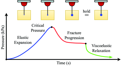
Figure 1: VCCE protocol: constant fluid injection via a needle-based system to recover the fully nonlinear response of a material under local loading conditions.

II.1 Verification via neo-Hookean Material Model

For validation of our bench-top unit, we use PDMS, which has previously been shown Raayai-Ardakani et al. (2019) to be well-characterized by the neo-Hookean model Gent and Lindley (1959) in the quasi-static range. For this, we first define the circumferential stretch, $\lambda$:

$$\lambda=\frac{{a}}{A},$$ (1)

where the effective radius of the spherical cavity, $a$, is divided by the effective initial defect radius, $A$. As shown in earlier studiesRaayai-Ardakani et al. (2019), the initial defect, and subsequent expanding cavity, is well captured by the spherical assumption. For this, we define the cavity, as an effective sphere, that expands to effective radius, $a$, in a soft material of undeformed radius, $B$, which under the influence of pressure, $p$, deforms to effective radius, $b$ (Fig.2).

Figure 2: An incompressible cavity expanding within an incompressible material of modulus, $E$, exerting pressure, $p$, at the cavity site.

A result (Eq.2) from the neo-Hookean modelGent and Lindley (1959) that describes the elastic expansion of the PDMS will be used in our instrumentation validation. Additionally, reproducing a result from Shabnam et al in Fig.3, cases for varying ratios of $B/A$ are shown with their impact towards the $p/E$ response.

$$\frac{p}{E}=\frac{5}{6}-\frac{2}{3\lambda}-\frac{1}{6\lambda^{4}}$$ (2)

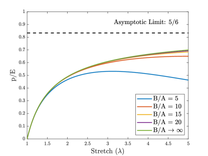
Figure 3: The role of sample size highlighted with respect to effective initial defect size for the neo-Hookean hyperelastic model.

For verification, we intend to produce fluid cavities of effective final radius, $a$=1.3mm, with effective initial defect sizes, $A$$\approx$0.25mm, corresponding to $\lambda$$\approx$5. In order to neglect boundary effects in our analysis, and particularly in fracture progression, we need sample sizes of $B/A$$\approx$20 indicating $B$$\approx$5mm as sufficient (Fig.3). Notably, if our focus were solely on presenting elastic data, specifically where $\lambda$$\approx$2, it would be adequate to concentrate on cases where $B/A$$\approx$10 and $B$$\approx$2.5mm.

For the result in Eq.2, the relationship between the system pressure, $p$, and the elastic modulus, $E$, manifests an asymptotic trend. As the pressure increases, it approaches a limit at 5/6 $E$. Given this result does not encompass fracture, it is difficult to ascertain the explicit range of stiffnesses VCCE may immediately apply. For this, we limit our attention to materials exhibiting critical pressures upwards of 100kPa prior to fracture.

III Instrumentation

This instrument, constructed using readily available components and costing less than $5000 USD, streamlines the evaluation soft materials using the VCCE method. The system can evaluate soft materials across a wide range of elastic moduli: 1, 10, and 100+ kPa, bringing VCCE testing within reach of users with limited technical background. Significantly, this instrument ensures errors remain below 5% for both measures of volume and pressure up to 100kPa, even at a material’s critical pressure where errors peak.

This system decomposes VCCE into two parimary subsystems: mechanical and electrical. Details on these subsystems and their components are provided below.

III.1 Bench-top Overview

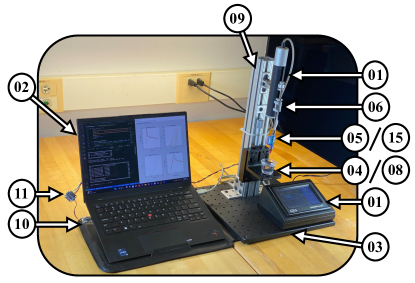
Figure 4: Assembled bench-top VCCE unit with major components listed in Table 1.

Table 1: Bill of Materials

[##]	Component Name	QTY
[01]	UMP3T & Controller w/ USB Cable	1
[02]	Laptop Computer	1
[03]	Optical Breadboard Baseplate	1
[04]	Translation Stage with Standard Micrometer	1
[05]	PendoTech Pressure Sensor	1
[06]	Hamilton 10$\mu$L Syringe	1
[07]	Aluminum Bolt-Together Corner-Bracket	5
[08]	Right-Angle Bracket with Counterbored Slots	1
[09]	T-slotted Framing Rail	1
[10]	RP2040 USB Key	1
[11]	Nuvoton NAU7802 24-Bit ADC	1
[12]	$\frac{1}{4}-20$ Socket Head Screws	18
[13]	T-Slotted Framing Fasteners	14
[14]	QT-to-QT Cable	1
[15]	25G Luer Lock Connection Needle	1
[16]	Water:PBS (9:1) Solution	0.4g

The bench-top system, as depicted in Fig.4 and with components shown in Table 1, is presented here in a high-level overview. The system is designed to work with laptop computers equipped with a minimum of two USB Type-A ports. Specifically, these ports are allocated for distinct functions: one for data acquisition - particularly pressure data - and the other for managing controls hardware. Data acquisition is facilitated through a PendoTech pressure sensor, connected to a 10$\mu$L syringe. This sensor is sequentially connected to an analog-to-digital converter and then a microcontroller-based USB key. The USB key, once inserted into the laptop computer, is accessed and controlled via Python scripting in Visual Studio Code, enabling data collection.

The selected hardware components include commercially available syringe microinjector systems from World Precision Instruments (WPI), specifically the UMP3T and MICROTOUCH 2T models. These systems are directly connected to the latop computer through USB and interrogated via the same Python scripting that handles data collection. Simultaneous data acquisition through two USB ports enables the synchronization of pressure readings with fluid expelled into the soft material. The proper correlation of pressure to volume generates accurate nonlinear response profiles for tested materials.

Before initiating data collection, the bench-top frame requires assembly. The microinjector subassembly is mounted onto a T-slotted framing structure, stabilized by an optical breadboard baseplate. Positioned directly beneath the microinjector subassembly and affixed to the T-slotted frame is a rack-and-pinion translation stage, outfitted with an embedded micrometer acting as the sample stage. This stage raises the soft material and inserts the needle into the sample in preparation for a VCCE test. The process of elevating the stage to introduce the sample into the needle elaborated in Section IV.2, is designed to create an initial cavity within the material, establishing a consistent and repeatable zero-condition for subsequent material analysis. Once inserted, a VCCE test may be performed and is outlined in greater detail in Section IV.

III.2 Soft Materials & Structural Compliance

In VCCE testing, maintaining minimal system compliance is crucial due to the nature of soft, viscoelastic materials, which are sensitive to changes in testing conditions due to instrumentation compliance. During a VCCE test, the material under examination is effectively in series with the system’s structure. As a result, when a load is applied, deformation occurs in both the material and the system, analogous to springs in series, impacting accuracy. To mitigate this, our design incorporates rigid materials, such as aluminum and steel. For elements that necessitate flexibility, like pressure sensors, we confirm that their influence on the overall system stiffness is negligible, especially relative to the test materials. This approach also prompts us to characterize the compliance of "incompressible" fluids and assess its impact on our specific system.

III.3 The Mechanical Subsystem

The mechanical system can significantly affect the data collected. Deformations in the mechanical subsystem during operation lead to losses in volume measurement. Hence, it is essential to evaluate each component within the subsystem to gauge their impact.

Assessing mechanical subsystem underpinning the VCCE methodology begins with examination of the instrument’s structural framework. This encompasses all structural components, including fastening hardware. For this, materials having a hardness greater than or equal to aluminum were chosen. These components are characterized by an approximate Young’s Modulus, denoted as $E$, equating to 70 GPa. When considering compliance within our instrument, we are only concerned with the dynamic, or operating state, where a liquid cavity is introduced into the soft material. During this transition, the needle tip bears the primary load, causing downstream components to undergo deformation—albeit to a lesser extent than the needle itself. This phenomenon results in a measurable deflection, symbolized by $\delta$, across a components cross-sectional area, $A$, which should be evaluated under maximum operational conditions. We have the capability to test our system up to the sensor’s maximum pressure of 500kPa; however, the peak pressures of most soft materials rarely reach such levels before fracture, even if their elastic modulus surpasses that figure. Therefore, we focus our analysis on local peak pressures up to 100kPa.

In complex systems, such as syringe microinjectors, it is important to examine how forces are transmitted from soft materials through pressure sensors, syringes, and motor assemblies - referred to here as the syringe subsystem - separate from the larger structural loop. The system reaction forces are mainly at the points of force application, with the syringe subassembly being the primary site of these interactions.

In our system, focusing on the forces local to the microinjector, we start by analyzing the syringe plunger. In operation, the observed volumetric losses arise from axial compression. To understand this, we use the following deformation relationship to evaluate the force due to the cavity growth, $F$, and length of the plunger, $L$:

$$\delta=\frac{FL}{AE},$$ (3)

Subsequently deriving the volumetric loss in operation due to axial compression, $\Delta{V_{c}}$, as follows:

$$\Delta{V_{c}}=\frac{FL}{E}.$$ (4)

In Table 2, the aluminum Hamilton 10$\mu$L syringe plunger, exhibits negligible volumetric losses at local pressures of 100kPa. Based on this, if the Young’s modulus of a component material, $E_{c}$, compared to the expected value for a tested soft material, $E_{s}$, yields a ratio $\frac{E_{s}}{E_{c}}$ significantly less than one (i.e., $\frac{E_{s}}{E_{c}}<<1$), the component is expected to have a negligible impact on the pressure-volume response.

Additionally, a secondary source of measurement compliance, and system failure, associated with the syringe plunger would be buckling. Buckling within the syringe was assessed using Euler’s critical load equation (Eq.5), focusing on the critical length at which buckling might occur under peak operating forces, $F_{c}$. Given area moment of inertia, $I$, and the effective length factor, $K$, we consider Euler’s critical load for syringe plungers exhibiting (1) rotation-fixed, translation-fixed, and (2) rotation-fixed, translation-free end conditions, resulting in a theoretical $K$ of 1.0 or recommended design value of 1.2 for $K$:

$$F_{c}=\frac{\pi^{2}EI}{KL^{2}}.$$ (5)

Frictional forces, primarily between the Teflon-coated glass syringe walls and the aluminum plunger, significantly contribute to the peak force, estimated at 1.0N Roth (2020). The operational state, under peak cavity expansion forces ($\sim$0.02N) and frictional forces, yields an effective buckling length of 80.7mm at 5kPa, 80.3mm at 50kPa, and 80.0mm at 100kPa, which are considerably beyond the syringe plunger’s maximum length of 65.0mm, mitigating buckling concerns.

Note that observations indicate buckling phenomena within the syringe plunger occur after the system has been idle for an extended period, typically spanning weeks. This interval allows for the evaporation of the Water:PBS solution, hereafter referred to as PBS, leading to salt deposits at the interface between the syringe plunger and the glass syringe body. Such accumulation markedly increases the system’s expected frictional forces elevating buckling risks. Therefore, if the unit is to be left unattended for weeks, it is recommended to disassemble and empty the syringe subassembly.

Evaluating the pressure sensor - the internal MEMS component - at high pressures, will follow a deflection profile similar to those found in Kirchoff-Love Plate Theory Love (1888) where the deflection, $w$, of a thin-disc of height, $h$, and the load the disc experiences, $q$, follows:

$$\nabla^{4}{w}=\frac{-q}{D},$$ (6)

where, $D$, is the flexural rigidity of our system and follows:

$$D=\frac{Eh^{3}}{12(1-\nu^{2})}.$$ (7)

Assuming the MEMS diaphragm is axisymmetric, $\frac{\partial}{\partial{\theta}}=0$, and that our distributed load is uniform, the equation reduces to:

$$\frac{1}{r}\frac{\partial}{\partial{r}}(r\frac{\partial}{\partial{r}}(\frac{1}{r}\frac{\partial}{\partial{r}}(r\frac{\partial{w}}{\partial{r}})))=\frac{-q}{D},$$ (8)

which, when applying clamped boundary conditions at $w=\frac{\partial{w}}{\partial{r}}=0$ for ($r=a$) (where $a$ is the radius of the MEMS diapgrahm), and knowing the stress must remain finite ($\frac{\partial^{2}{w}}{\partial{r^{2}}}$), the deflection profile for our clamped-clamped thin disc reduces to the following:

$$w=\frac{-q}{64D}[(r^{2}-a^{2})^{2}].$$ (9)

Integrating over the surface of the diaphragm yields the following Kirchoff-Love volumetric change equation:

$$\Delta{V_{MEMS}}=\frac{-\pi{a^{6}q}}{192D}.$$ (10)

In Table 2, for the MEMS diaphragm with a radius of 1mm and thickness of 0.1mm, the measured volumetric losses are 0.5nL at a peak pressure of 5kPa, 4.7nL at 50kPa, and 9.5nL at 100kPa. These findings suggest a negligible impact for samples experiencing peak pressures within the 50kPa range; however, the significance of volumetric loss begins to increase for samples that may encounter peak pressures of 100kPa.

Table 2: Table of notable volumetric losses in structure and system as pressure increases in samples collected. Components are from Table 1.

[##]	Eq.	$E$ (Pa)	$\nu$	$K$ (Pa)	$\Delta{V_{5kPa}}$ (nL)	$\frac{\Delta{V_{5kPa}}}{<V_{c}>}$ (%)	$\Delta{V_{50kPa}}$	$\frac{\Delta{V_{50kPa}}}{<V_{c}>}$	$\Delta{V_{100kPa}}$	$\frac{\Delta{V_{100kPa}}}{<V_{c}>}$	$\frac{E_{s}}{E_{c}}$
[05]	(14)	2.4e9	0.35	–	0.5	0.1	4.5	1.2	9.1	2.4	2.5e-4
[05]	(10)	5e6	0.48	–	0.5	0.1	4.7	1.3	9.5	2.5	0.1
[06]	(14)	60e9	0.20	–	2.5e-3	6.5e-4	2.5e-2	6.5e-3	5.0e-2	1.3e-2	1.0e-5
[06]	(4)	70e9	–	–	1.19e-3	3.1e-4	1.2e-2	3.1e-3	2.4e-2	6.1e-3	8.6e-6
[15]	(14)	1.5e9	0.42	–	0.4	0.1	3.7	1.0	7.4	2.0	4.0e-4
[15]	(14)	193e9	0.29	–	6.8e-5	1.8e-5	6.8e-4	1.8e-4	1.3e-3	3.6e-4	3.1e-6
[16]	(15)	–	–	2.22e9	0.9	0.2	9.0	2.4	18.0	4.8	–

In syringe microinjector systems, interaction between the internal motor and an attached syringe generates a pulsatile flow effect which arises as harmonic compliance in the nonlinear response. This necessitates the selection of a syringe that minimizes this phenomenon. For a 10$\mu$L Hamilton syringe, the flow regime for this instrument, especially at maximum fluid volume rates, $Q$, of 657$\frac{nL}{s}$, is viscous for a PBS solution. This is determined based on its dynamic viscosity, $\mu$, of 1.0mPa-s, density, $\rho$, of 1000$\frac{kg}{m^{3}}$, and diameter, $D$, of 0.3048mm:

$$Re=\frac{\rho UD}{\mu}=2.74,$$ (11)

Which indicates a laminar flow profile as characterized by the Reynolds number, $Re$. The implementation of ball bearings within syringe microinjector stepper motors enhances precision Fukada, Fang, and Shigeno (2011); however, those same bearings introduce harmonic oscillations Saruhan et al. (2014), observable within pressure measurements. This interaction between motor dynamics, transient inertial forces, and viscous forces is described by a material’s density, $\rho$, the frequency of the pulsatile flow, $\omega$, and the characteristic radius, $R$, through the dimensionless Womersley number, $\alpha$:

$$\alpha=R\sqrt{\frac{\omega\rho}{\mu}},$$ (12)

where, $\alpha$, highlights the balance between oscillatory inertial effects and viscous forces within the flow. The significance of $\alpha$ in syringe diameter selection becomes evident: a large diameter may amplify transient inertial effects, thereby distorting measurements, whereas an excessively small diameter risks injecting insufficient fluid volumes, reducing how much of the material’s nonlinear response is recovered.

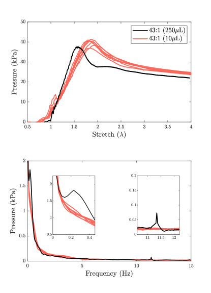
Figure 5: The impact of varying the syringe size from 10$\mu$L (red) to 250$\mu$L (black) within VCCE protocols and how undesirable frequencies begin to emerge and impact the overall measurement of soft materials.

In assessing the impact of syringe diameter on a cost-effective VCCE system, a comparison between 250$\mu$L and 10$\mu$L syringes was performed. This comparison evaluated a 43:1 PDMS sample at $Q$=300$\frac{nL}{s}$.

In Fig.5, the pressure-stretch response reveals a prominent, slowly varying signal of significant magnitude at low stretches, suggesting a perceived increase in material stiffness at lower stretch values. This area is critical for the application of constitutive models, especially the derived result from the neo-Hookean model (Eq.2). Additionally, the emergence of the higher-frequency signal may affect the system’s signal-to-noise ratio; however, this is of lesser concern relative to the lower-frequency signal. Especially at lower stretches where constitutive models are most applicable, the 250$\mu$L syringe presents significant challenges in recovering material properties, due to pulsatile flow effects of frequency 0.23Hz. Larger stretch values ultimately align with the dataset’s equilibrium, suggesting the initial flow characteristics are transient and diminish over time; however, this equilibration manifests late in the pressure response, highlighting the importance of minimizing syringe volume to enhance precision in diagnostics and model fitting.

For this, a Hamilton 1700 series gas-tight syringe, specifically the 10$\mu$L variant, was utilized. In terms of volumetric loss observed during operation, the syringe body can be analogized to a thick-walled pressure vessel with borosilicate glass’s material properties, $\nu$ being 0.2, and $E$ being 60GPa. This body was with external, $P_{o}$ and internal pressures, $P_{i}$, and respective radii, $r_{o}$ and $r_{i}$:

$$\Delta{r}=\frac{1-\nu}{E}\left(\frac{P_{i}r_{i}^{2}-P_{o}r_{o}^{2}}{r_{o}^{2}-r_{i}^{2}}\right)r+\frac{1+\nu}{E}\left(\frac{(P_{i}-P_{o})r_{i}^{2}r_{o}^{2}}{(r_{o}^{2}-r_{i}^{2})r}\right)$$ (13)

$$\Delta{V_{s}}=\pi h_{s}\left(\Delta{r_{r_{i}}}^{2}+2\Delta{r_{r_{i}}}r_{i}-2\Delta{r_{r_{o}}}r_{o}-\Delta{r_{r_{o}}}^{2}\right).$$ (14)

Evaluation at pressures of 5kPa, 50kPa, and 100kPa revealed that volumetric losses were assessed to be less than one nanoliter, as detailed in Table 2, indicating that the syringe body’s contribution to measurement inaccuracies was negligible. This study was extended to include analysis of components such as the needle and the luer-tipped needle connector, which are constructed from stainless steel 304 and polycarbonate, respectively. The evaluation indicates negligible radial volumetric losses for the stainless steel 25G needle, while the polypropylene luer-tipped needle exhibits greater losses of 9.1nL at critical pressures nearing 100kPa (Table 2). For the polypropolene luer-tipped needle connector, this value is likely overestimated due to the presence of reinforcing longitudinal ribs and a tapered geometry that was not accounted for. Additionally, the PendoTech pressure sensor, which expands radially and is made of polycarbonate material with a Young’s modulus of 2.4 GPa and a $\nu$ of 0.35, yields results comparable to those of the polypropylene luer-tipped needle connector (Table 2). At a critical pressure of 100 kPa, the deformation is measured at 9.1nL, which is similarly negligible. Nonetheless, this acknowledges the potential for deformation of less rigid components to influence the overall accuracy of diagnostic outcomes.

The last component to be assessed is the PBS solution. Specifically, we are interested in its compressibility at peak operating pressures. Utilizing the bulk modulus, $K$, of water at 2.22GPa, and an initial volume of PBS, $V_{o}$, of 0.40g, the compressibility of the PBS solution can be calculated as follows:

$$\Delta{V_{w}}=-\frac{P{V_{o}}}{K}.$$ (15)

In Table 2, the PBS, contributes to a perceived volumetric loss in measurement of 0.9nL at peak pressures of 5kPa, 9.0nL at 50kPa, and 18.0nL at 100kPa, with 4.8% measurement error at peak operating pressures. The findings reveal that samples subjected to peak pressures within the 50kPa range are minimally affected; however, the significance of volumetric loss becomes more pronounced at peak pressures approaching and exceeding 100kPa. In many systems, PBS’s compressibility is negligible and can usually be overlooked until measurements are taken at significantly higher peak pressures, at which stage detailed post-processing is required to separate water compressibility effects from the properties of the soft material.

III.4 The Electrical Subsystem

III.4.1 Pressure Sensing Configuration

The initial component of the electrical subsystem incorporates a PendoTech single-use pressure sensor, designed to measure both static and dynamic pressures of gases and liquids. The sensor operates via a Wheatstone bridge configuration Hoffmann (1974), where pressure is recorded through balancing a resistor bridge, and correlating the change in resistance (or voltage) at equilibrium, to a measure of pressure.

The specific sensor used, is capable of measuring pressures ranging -11.5 to 75 psi. The claims regarding the variability and accuracy of the sensor are crucial because they impact results by influencing the measurement of pressure. The sensor’s accuracy is delineated as follows: $\pm$2% for the 0 to 6 psi range, $\pm$3% for the 6 to 30 psi range, and $\pm$5% for the 30 to 60 psi range. Notably, the sensor’s accuracy claims extend only to 60 psi (413.7kPa), necessitating caution beyond this threshold. Experiments within the 60-75 psi range should be conducted with sensors calibrated against verified pressure gauges to ensure reliability.

III.4.2 Signal Processing and Power Supply

Signal conversion from the MEMS-based PendoTech pressure sensor to a computer-interpretable format is achieved using Nuvoton’s NAU7802, a 24-Bit Analog-to-Digital Converter (ADC) specifically designed for Wheatstone bridge sensors. The digital output is interfaced with a RP2040 microcontroller embedded USB Key, which facilitates data transmission to the host computer via serial communication. Power to the pressure sensor is provided directly from the host computer’s USB port, with voltage regulation provided by the RP2040 microcontroller, ensuring compatibility with the Inter-Integrated Circuit (I2C) communication protocol. To minimize the signal-to-noise ratio of the measurements, the operating voltage should be minimized. In this setup, an unregulated 5.00VDC from a USB port is first regulated down to 3.30VDC within the RP2040, and then further reduced to 3.00VDC for the pressure sensor. This is achieved using a single cable path and USB port. The received signal, in volts, is converted to a measure of pressure via the following conversion 0.2584mV/V/psi where the supply voltage used for calculation is 3.00VDC.

Further, calibration would be necessary if the temperature of the system were varying in time. To this end, we begin all tests through writing to the Nuvoton ADC 0x11 hexadecimal register and enabling temperature sensing. We record temperature. then automatically archive the value in our master test logs for each test. Checks between tests should be performed to ensure that temperature is constant throughout. If not, a correction factor of 0.3$\frac{mmHg}{C}$ becomes necessary when temperature varies.

IV Methods

IV.1 PDMS Fabrication Procedure

PDMS samples were prepared utilizing base:crosslinker ratios of 43:1, 45:1, and 47:1. The elastomer formulation was Sylgard 184. Each ratio mixture was separately processed in 150mL resin containers, designed for compatibility with the Thinky SR-500 planetary mixer, creating a homogeneous blend of components.

The PDMS base and crosslinker mixtures were subjected to a comprehensive two-phase mixing regimen within the planetary mixer. Each phase consisted of a 30-second mix at a controlled speed to ensure thorough integration of the base and crosslinker without introducing excessive air bubbles.

Following the mixing process, the homogenized PDMS was immediately transferred to a vacuum chamber. The degassing stage removed entrapped air and helps to avoid bubble formation within the material. Subsequently, the degassed mixture was poured into disposable plastic 2oz cups.

The filled 2oz containers were then placed in a curing oven set to 100C for a duration of two hours. This curing protocol was optimized to facilitate a complete cross-linking reaction. Samples were then allowed to rest at room temperature for eight days post-curing. This additional resting period was to ensure any residual crosslinking reactions were complete, stabilizing the material’s properties while minimizing potential long-term stiffening effects that could arise in PDMS.

IV.2 Testing Protocol

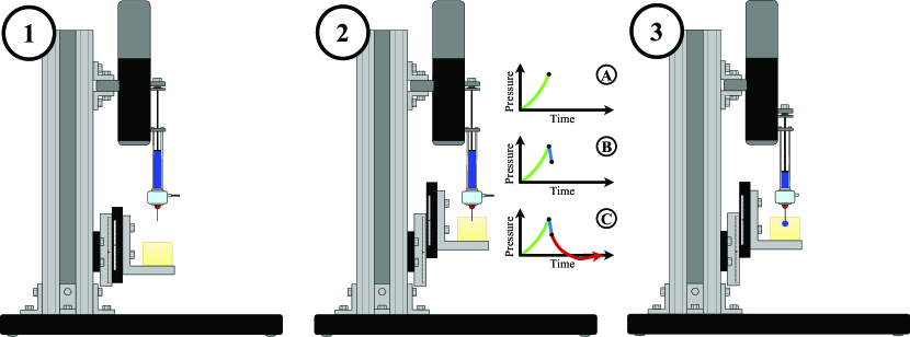
Figure 6: VCCE testing is performed in three stages: 1) loading a sample on the translation stage, 2) raising the translation stage into the syringe assembly and 2.A-C) zeroing pressure, and lastly, 3) control the rate of cavity creation within the material.

Data acquisition and motor control in our system are managed through a Python script, VCCE_CONTROL_CODE.py, run in Visual Studio Code. This script integrates both controls and data acquisition, streamlining the experimental process.

For new users, it’s necessary to download and install the latest firmware for the RP2040 USB key. This firmware has been archived and can be found in the Nonlinear Solid Mechanics Group GitHub. Once the firmware is installed, and other supporting materials for this project are downloaded/installed, the setup is complete, and the system is ready for use.

Before conducting experiments on soft materials, a dynamic calibration test with PBS is essential to account for any potential losses due to fluid and frictional forces (Fig.7) which are averaged and subtracted out from the final soft material datasets. This involves placing the PBS solution in direct contact with the syringe needle where the syringe needle is slightly under the PBS surface and running the VCCE_CONTROL_CODE.py script. Users will be guided through the VCCE process and then prompted to select the desired testing parameters for this initial calibration. In the context of this study, we selected a constant volumetric flow rate of 300$\frac{nL}{s}$ for a final cavity radius of 1.3mm. Following these selections, the test commences, with data saved to the TEST_DATA folder directory for later post-processing.

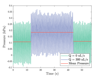
Figure 7: Measured PBS calibration for a 10$\mu$L syringe at 300$\frac{nL}{s}$.

Once the initial water calibration is completed, the testing of soft materials can commence. Microinjector systems, characterized by their bi-directional motor functionality, necessitate a specific minimum engagement distance between the syringe plunger carrier and the threaded rod that connects to the stepper motor. For the WPI UMP3T setup, this distance is approximately 100$\mu$m. Utilizing a 10$\mu$L syringe as the test instrument, the system requires an advancement of approximately 34.5 steps to begin testing, with each step dispensing approximately 0.6nL, totaling an approximate 20nL of fluid expulsion before the initiation of any tests. Upon activation of the VCCE_CONTROL_CODE.py, the motor is programmed to move approximately 50nL at a delivery rate of 100$\frac{nL}{s}$ to prime the system. Adjustments for larger syringe volumes are facilitated through modifications to the primeMotor() function within the script. Following this preliminary step, the ADC is calibrated to zero to reflect current environmental conditions.

Table 3: Insertion Procedure Data – Distance Traveled

Sample	$z_{p}$ (mm)	$z_{f}$ (mm)	$z_{r}$ (mm)	$z_{t}$ (mm)
43-1	-12.0	-5.0	+5.0	-12.0
43-2	-15.0	-5.0	+4.0	-16.0
43-3	-15.0	-5.0	+5.0	-15.0
43-4	-13.0	-5.0	+5.0	-13.0
43-5	-12.0	-5.0	+4.0	-13.0
43-6	-15.0	-5.0	+4.0	-16.0
43-7	-15.0	-5.0	+4.0	-16.0
45-1	-15.0	-5.0	+5.0	-15.0
45-2	-15.0	-5.0	+4.0	-16.0
45-3	-16.0	-5.0	+4.0	-17.0
45-4	-15.0	-5.0	+5.0	-15.0
45-5	-17.0	-5.0	+4.0	-18.0
45-6	-15.0	-5.0	+4.0	-16.0
45-7	-15.0	-5.0	+4.0	-16.0
47-1	-17.0	-5.0	+5.0	-17.0
47-2	-17.0	-5.0	+4.0	-18.0
47-3	-16.0	-5.0	+5.0	-16.0
47-4	-15.0	-5.0	+5.0	-15.0
47-5	-16.0	-5.0	+4.0	-17.0
47-6	-15.0	-5.0	+4.0	-16.0
47-7	-17.0	-5.0	+4.0	-18.0

The needle insertion process involves real-time pressure feedback displayed in the Visual Studio Code terminal. The idealized pressure response as a needle inserts a soft material, prior to testing, may be seen in Fig.6.2.A-C, where Fig.6.1-3 outlines the VCCE testing procedure. In Fig.6.2.A, the green region represents the needle being inserted into the material, depressing the surface of a material, but the needle has not been fractured the material surface yet. In Fig.6.2.B, the blue region represents when the needle has fractured the material surface, after a distance, $z_{p}$ (Table 3), and a near instantaneous drop in pressure is seen. To increase adhesion between the needle surface and material, the needle is further plunged a distance, $z_{f}$ (Table 3), into the material. Afterwards in Fig.6.2.C, the needle is slowly retracted, by a distance, $z_{f}$ (Table 3), until the pressure reaches zero. The total distance traveled relative to the material surface for each insertion, $z_{t}$, may be seen in Table 3. Completing the insertion procedure, an initial defect is created, which will be the basis for constitutive analysis. It also indicates that the testing setup is prepared for fluid injection and the subsequent VCCE testing as seen in Fig.6.3.

After completing the needle insertion procedure, the user enters the main VCCE testing protocol. Here, the user may opt for radial control, which governs the expansion of the cavity by its radius, or volumetric control, which governs expansion by total volume of fluid per unit time. Although radial control can provide a more precise measure of a material’s true elastic modulus, its implementation is not common for COTS microinjector systems due to their discrete control biases.

Given the UMP3T’s architecture as a discrete control system, a form of segmented volumetric control (pseudo-radial control) has been developed and is available for use at our GitHub; however, this approach is generally discouraged as the MICROTOUCH controller can introduce delays of 0.2 seconds as it processes new commands. Therefore, for the sake of consistency and to mitigate the controller’s limitations, constant volumetric control was employed throughout the experiments. Each test maintained a steady flow rate of 300$\frac{nL}{s}$ until reaching a predefined cavity radius of 1.3mm, equivalent to a total injection volume, $V_{T}$, of 9202.8nL. Following injection, a 60-second relaxation period for the material was allowed, enabling observation of viscoelastic relaxation.

Post-experiment, the data was archived for processing. The entire testing sequence was executed 21 times, in direct succession, to ensure reliability and repeatability.

V Results, Validation, & Discussion

Data were collected and analyzed from 21 consecutive tests, spanning samples with PDMS base to crosslinker ratios of 43:1, 45:1, and 47:1 (Fig.8). Each ratio group was represented by 7 distinct tests, designed to elucidate key mechanical properties from the elastic expansion, critical pressure, and fracture progression (Fig.1). Comprehensive datasets, encompassing all collected data and further observations on viscoelastic relaxation, are accessible via the GitHubcohen-mechanics group (2024).

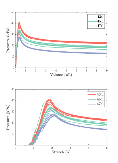
Figure 8: Material response curves for 21 successive tests of testing PDMS of ratios 43:1 (red), 45:1 (green), and 47:1 (blue) for both $p-v$ response curves and $p-\lambda$ curves.

The samples collected, nearly indistinguishable in their stiffness by human touch, exhibit clear trends prior to constitutive fitting (Fig.8). Quantitatively, parameters that can be derived, such as the volume at which the material fractures, $V_{c}$, energy up until fracture, $U_{c}$, critical pressure before fracture, $P_{c}$, and total energy within the system, $U_{s}$, are documented in Table 4 for each sample collected. The local maxima of the datasets, $P_{c}$, are observed to decrease with an increase in the base to cross-linker ratio in PDMS, suggesting a correlation between material stiffness and critical pressure preceding fracture onset. Specifically, the average critical pressures for ratios of 43:1, 45:1, and 47:1 are 39.76$\pm 1.54$kPa, 34.12$\pm 2.23$kPa, and 27.57$\pm 1.70$kPa, respectively. These values reflect the decreasing energy threshold the sample can endure prior to fracturing. Moreover, the PDMS material is noted to fracture at volumes measured in nanoliters, with the 43:1 ratio fracturing at an average volume of 390.6$\pm 45.3$nL, 45:1 at 374.5$\pm 38.9$nL, and 47:1 at 366.1$\pm 19.1$nL.

By employing numerical integration of the PDMS results up to the critical pressure, we are able to calculate the total energy within the system prior to fracture:

$$U_{c}=\int_{0}^{V_{c}}p\,dV.$$ (16)

Additionally, we are able integrate the entire nonlinear response, up until the total volume injected, $V_{T}$, to represent the total energy within the system:

$$U_{s}=\int_{0}^{V_{T}}p\,dV.$$ (17)

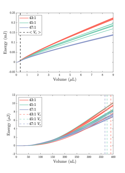
Figure 9: Cumulative energy within the system evaluated through the nonlinear response of the material, $U_{s}$ (top), and available energy within the system evaluated up until fracture, $U_{c}$ (bottom), with average volumes of fracture for each PDMS ratio indicated.

Displaying the cumulative integration yielding $U_{s}$ and $U_{c}$ in Fig.9, with top plot depicting $U_{s}$, and bottom plot depicting $U_{c}$, we observe the energies of each sample converging as volume increases. Particularly, in the top figure, we observe that the average volume at which all samples fractured, $<V_{c}>$, represents only a small fraction of the total dataset. Further analysis of this minor portion reveals significant overlap in energies, with groupings beginning to form right at the average values of $V_{c}$ each material fractured.

Figure 10: Energy within the system evaluated through the nonlinear response of the material, $U_{s}$ (top), and available energy within the system evaluated up until fracture, $U_{c}$ (bottom).

Further, showing the distribution of energy in Fig.10, for both $U_{s}$ (top) and $U_{c}$ (bottom), we see the instrument performs well in being able to differentiate materials based on their ability to sustain energy due to in-vivo loading conditions when evaluating over the entire nonlinear response, particularly, 43:1 yielded, $U_{s}$, equal to 0.23$\pm$0.003mJ, 45:1 equal to 0.19$\pm$0.009mJ, and 47:1 equal to 0.14$\pm$0.002mJ. When focusing on the region before fracture, the system still effectively groups energy, and trends can be observed as 43:1 yielded, $U_{c}$, equal to 9.13$\pm$0.88$\mu$J, 45:1 equal to 7.72$\pm$0.90$\mu$J and 47:1 equal to 6.36$\pm$0.31$\mu$J. This outcome suggests this instrument may be useful in the biological domain for distinguishing between healthy and diseased tissue when a sufficiently large volume is expanded or understanding how material toughness varies with a host of variables, such as time since tissue resection, hydration of tissue, or even material toughness under different pre-load conditions.

In preparation for fitting a constitutive model, an examination was conducted to characterize the noise within the system, analyzed as a function of stretch (Fig.11). This was performed by implementing a moving mean filter across the original datasets and subtracting this output from the initial data to extract peak-to-peak noise levels. Subsequently, the resultant noise, expressed in terms of pressure, was categorized into bins based on stretch intervals of 0.25.

In Fig.11, it is seen at low stretches, and equivalently early times, that noise can be expected to be largest during measurement. This peak-to-peak noise, is attributed to dynamic events in the electronics subsystem. This effect has the potential to be mitigated by using slower volumetric flow rates than 300$\frac{nL}{s}$; however, it is later shown that 300$\frac{nL}{s}$ does not ultimately impact the region of stretch that was fit to the neo-Hookean model.

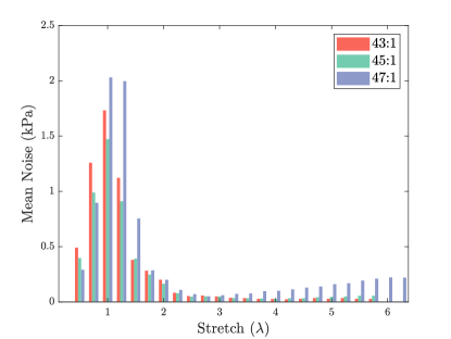
Figure 11: Mean peak-to-peak noise between the different samples depicted in $\lambda$ domains.

Additionally, an increase in system noise is observed as the material tested becomes softer. This phenomenon is also linked to the electrical subsystem components. It is hypothesized that the current sensing modality, which employs Wheatstone bridges to measure slowly varying signals, may possess inherent limitations for soft materials at higher stretches, where pressure is slowly varying. These limitations necessitate further investigation into different conversion modalities to enhance the accuracy and reliability of measurements in future studies. This insight underscores the importance of continuous improvement in the sensing technologies used for characterizing the mechanical properties of soft materials, especially if systems costs and form-factor are to remain competitive.

The data was subsequently analyzed utilizing the neo-Hookean constitutive model to attain a measure of the elastic modulus for each PDMS ratio tested. Specifically, the modulus reported throughout is an instantaneous elastic modulus, $E_{i}$, due to initially high stretch rate expansionsChockalingam et al. (2021). The fitting procedure remained consistent across all PDMS ratios. Initially, the dynamic pressure response obtained from the infusion of the PBS solution into another cup of PBS at a constant volumetric flow rate of 300$\frac{nL}{s}$ was subtracted from the PDMS data. Subsequently, the nonlinear results for PDMS were truncated between the geometric values of the effective radius, $a$, of the 25G needle (0.2575mm) and the radius of critical pressure for each sample. Point-pairs along the slope were identified and assessed to determine the segment with the highest slope, adhering to the principle that the point-pair method, when utilized to draw lines of best fit, serves as a smoothing technique across regions of interest. This approach is particularly effective for the linear, monotonically increasing elastic branch of the PDMS data.

The point-pair exhibiting the steepest slope was then extrapolated to identify the abscissa, which corresponds to a potential initial defect size, $A$. This initial value is necessary for the subsequent minimization to attain stretch, $\lambda$. Given the application of point-pairs as a pseudo-smoothing method to ascertain the initial defect size, it was necessary to retrieve the actual, raw data points within the delimited point-pair range. This retrieval of data, denoted the fitting region in Fig.12, was executed using a region of interest extraction, selecting the 55% mark within the accumulated dataset as a reference. The lower and upper bounds for the region of interest were set at 20% and 30% of its total length, respectively. These bounds, combined with the 55% data location, delineate the specific segment of the elastic branch for each sample that was subjected to fitting with the neo-Hookean model.

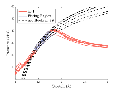
Figure 12: Highlighting the neo-Hookean fitting procedure for 43:1 PDMS samples. The fitting region, illustrates where the spherical cavity assumption holds true and is a region of high elastic energy.

As seen in Fig.12, the neo-Hookean model, while adept at describing the elastic properties of materials, falls short in capturing the fracture mechanics of hyperelastic materials subjected to large deformations. Thus, the utility of the neo-Hookean model is primarily confined to providing insights into the elastic characteristics of materials - the instantaneous elastic modulus for our validation.

To accurately determine the instantaneous elastic modulus, $E_{i}$, alongside a fitted initial defect size, $A$, and the corresponding stretch value, $\lambda$, the least-squares method was used:

$$\min_{\lambda,E}\sum\left(p_{i}-E\left(\frac{5}{6}-\frac{2}{3\lambda}-\frac{1}{6\lambda^{4}}\right)\right)^{2},$$ (18)

where, $p_{i}$, denotes the measured pressure values and $i$ encompasses the total count of observations over which the summation is executed. For the process of optimizing the model parameters, initial estimations are provided for the instantaneous elastic modulus, bounded between 1 and 500kPa. The initial guesses for the defect size are constrained by the bounds of the negative and positive values of the extrapolated point-pair abscissa exhibiting the largest slope. Through this constrained optimization approach, we are able to derive fitted values for the initial defect instantaneous elastic moduli, and stretch.

Table 4: Assembled experimental information of neo-Hookean fits, peak recorded pressures, and values of energy.

Sample	$V_{i}$ (nL)	$V_{c}$ (nL)	$\lambda_{c}$	$P_{c}$ (kPa)	$E_{i}$ (kPa)	$U_{c}$ ($\mu$J)	$U_{s}$ (mJ)
43-1	60.8	354.0	1.80	40.9	110.1	8.31	0.231
43-2	53.0	399.7	1.96	38.5	94.5	9.62	0.223
43-3	58.2	353.9	1.83	40.4	111.7	8.21	0.226
43-4	55.8	359.9	1.86	41.3	108.5	8.60	0.231
43-5	58.2	393.5	1.89	39.8	106.0	9.20	0.232
43-6	60.9	389.7	1.86	40.5	109.9	9.22	0.230
43-7	78.3	483.3	1.83	36.9	96.3	10.74	0.226
45-1	56.5	411.2	1.94	34.0	83.5	8.61	0.202
45-2	51.0	408.2	2.00	32.9	79.6	8.30	0.191
45-3	54.7	356.5	1.87	33.6	85.0	7.11	0.188
45-4	50.5	392.2	1.98	33.4	79.7	8.35	0.192
45-5	71.0	306.2	1.63	39.0	114.0	6.57	0.200
45-6	56.1	348.1	1.84	32.1	82.8	6.66	0.174
45-7	54.1	398.8	1.95	33.8	83.9	8.44	0.193
47-1	45.5	372.0	2.01	27.0	65.1	6.25	0.141
47-2	42.8	379.8	2.07	26.2	64.3	6.37	0.140
47-3	40.6	376.8	2.10	26.1	64.9	6.21	0.141
47-4	43.9	376.2	2.05	27.4	66.4	6.61	0.142
47-5	48.3	380.8	1.99	27.8	68.2	6.86	0.143
47-6	44.6	339.3	1.97	31.2	84.5	6.32	0.144
47-7	36.4	337.7	2.10	27.5	68.5	5.87	0.140

Fitted average values for the initial defect sizes, $A$, exhibit a downward trend with the values for 43:1 ratio being 0.243$\pm$0.010mm, for 45:1 being 0.237$\pm$0.009mm, and for 47:1 being 0.217$\pm$0.006mm. This observed trend suggests that softer materials may produce smaller initial defects, reflecting ease of defect formation. Similarly, critical stretch values, $\lambda_{f}$, indicative of the stretch at which fracture is presumed to occur, exhibit an upward trend as the material softens. Specifically, the average $\lambda_{c}$ values are 1.86$\pm$0.05 for the 43:1 ratio, 1.89$\pm$0.13 for the 45:1 ratio, and 2.04$\pm$0.05 for the 47:1 ratio. This pattern aligns with the expectation that softer materials can undergo greater deformation before fracturing.

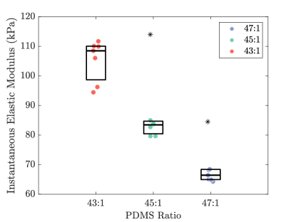
Figure 13: Box plots illustrating the instantaneous elastic modulus, $E_{i}$, for the 43:1 (red), 45;1 (green), and 47:1 (blue) PDMS ratios.

In Fig.13, the fitted instantaneous elastic moduli, $E_{i}$, demonstrate a decreasing trend as the base:crosslinker ratio in PDMS increases, which aligns with theoretical expectations. The average elastic modulus values for each PDMS ratio are 105.28$\pm$7.02kPa for 43:1, 86.91$\pm$12.12kPa for 45:1, and 68.84$\pm$7.10kPa for 47:1, differentiating the mechanical properties of the samples, even at low sample sizes ($N$=7).

An argument could be made regarding whether the samples labeled 45-5 and 47-6 constitute outliers in comparison to the remainder of the dataset (Table 4). At first glance, these values might seem anomalous; however, revisiting the energy discussion from earlier and looking at both $U_{s}$ and $U_{c}$ (Fig.10 & Table 4), we see their energies fall within acceptable ranges for similar base:crosslinker ratios with minimal overlapping in $U_{c}$ and no overlapping in $U_{s}$. This suggests that the discrepancy may not be due to inherent material properties, but rather extraneous factors, such as pre-test conditions, where material may have been lodged in the needle, adversely affecting the volumetric expansion process, or the sample exhibited discrepancies during the curing process.

In light of these considerations, the decision to retain these datasets in all calculations, rather than treat them as outliers was deliberate, even though their outlier treatment would greatly collapse the instantaneous elastic moduli results: 43:1 equaling 105.28$\pm$7.02kPa, and 45:1 equaling 82.40$\pm$2.24kPa, and 47:1 equaling 66.23 $\pm$1.77kPa. This serves to underscore the inherent variability encountered in testing soft materials. Despite such variability, the overall results maintain a general concordance with established trends and comparisons with analogous materials. Further, it highlights the potential utility of the energy metric as a cross-check for constitutive modeling or potentially even a stand-alone metric for material diagnostics. Thus, the inclusion of these datasets enriches the validation by providing a more nuanced understanding of the experimental challenges and the robustness of the findings, even in the face of potential procedural anomalies.

VI Summary and Conclusions

In this study, we have pioneered an innovative bench-top testing instrument for the VCCE method, specifically designed to advance the analysis of soft materials. This instrument stands as the first of its kind, transforming VCCE into a portable, user-friendly format suitable for space-constrained environments. Our development not only simplifies the VCCE testing process but also ensures accessibility without compromising on the accuracy or depth of material analysis. By examining PDMS samples across a range of base:crosslinker ratios, we validated instrument utility and simultaneously illustrate diagnostic utility of this instrument for broad audience adoption.

This instrument marks a significant step forward in soft material characterization and opens opportunities for further improvements. Recent advancements in VCCE, such as adopting continuous control through Dynamic Instron machines, suggests pathways to enhance radial fluidic injection rates into soft materials. While this current setup faces limitations in achieving continuous control due to the main microinjector component, future designs focusing on reduced reliance of proprietary microinjectors will overcome this challenge.

The introduction of a bench-top VCCE instrument represents crucial advancement in the understanding of soft material mechanics. It facilitates deeper material property insights and promise new research avenues, aiming to improve both theoretical and practical approaches in soft material science. As we look ahead, the continued evolution of this technology and methodology will undoubtedly yield significant contributions to the field, enhancing our ability to explore and understand the complex world of soft materials.

CRediT authorship contribution statement

Brendan M Unikewicz: Writing – review & editing, Writing – original draft, Visualization, Validation, Software, Design, Methodology, Investigation, Formal analysis, Data collection & curation, Conceptualization Andre M Pincot: Writing - review & editing, Writing - draft methodology, figure captions, figure curation, Supplementary data collection & curation Tal Cohen: Writing – review & editing, Supervision, Methodology, Funding acquisition, Conceptualization

Declaration of Competing Interest

The authors declare that they have no known competing financial interests or personal relationships that could have appeared to influence the work reported in this paper.

Data Availability

The data that support the findings of this study are openly available in our GitHub:

github.com/cohen-mechanics-group/cots-benchtop-vcce

Appendix A Appendixes

A.1 Boundary Effects in the neo-Hookean Model

Shabnam et al, 2019, showed the influence of boundary effects in the neo-Hookean model. Defining the circumferential stretch at the boundary as $\lambda_{b}$:

$$\lambda_{b}=\frac{b}{B}\left[\left(1+\left(\lambda^{3}-1\right)\right)\left(\frac{A}{B}\right)^{3}\right]^{1/3}.$$ (19)

The undeformed and deformed states of a material body are characterized by their respective inner and outer radii, $A$ and $B$ for the undeformed configuration, and $a$ and $b$ for the deformed configuration. The ratio, $\frac{B}{A}$, captures the relationship between the size of the boundary and the initial defect size. This ratio’s significance is underscored in our investigation of boundary effects on material stretch during assumed cavitation events. To this end, we employed multiple $\frac{B}{A}$ ratios, aiming to elucidate their impact on the anticipated stretch values within various cavitation geometries:

$$\frac{p}{E}=\frac{1}{6}\left(\lambda_{b}^{-4}+4\lambda_{b}^{-1}-\lambda^{-4}-4\lambda^{-1}\right).$$ (20)

A.2 Structural Volumetric Losses: Beams and Columns

When considering the scaling of the instrument or if T-slot framing and fasteners are shown to deform significantly, a thorough evaluation of the structural loop becomes important. While not pertinent for our proposed instrument, if readers opt for subtle differences in components and their assembly, the structure’s frame can be decomposed into two primary configurations: beams and columns. For an optimized representation of worst-case operational scenarios, beams are approximated with a uniform cross-sectional area and are considered to be purely end-loaded to maximize total deflection. Equations describing the perceived volumetric losses in measurement, for the beam and column orientations, as you move along a direction, $x$, are thus:

$$\delta(x)=\frac{Fx^{2}}{6EI}(3L-x),$$ (21)

which, upon integration, translates to a total volumetric loss for cantilever beams, $\Delta{V_{b}}$:

$$\Delta{V_{b}}=\frac{1}{8}\frac{FL^{4}}{EI}w,$$ (22)

where the area moment of inertia, $I$, is defined as $I=\frac{bh^{3}}{12}$ for a square cross-section with side lengths $b=h$. In the context of columns, particularly the main post subjected to a moment, $M$, at each end, the deformation is described by:

$$\delta(x)=\frac{Mx^{2}}{2EI}.$$ (23)

Leading to a volumetric change, $\Delta{V_{p}}$, for post members (columns):

$$\Delta{V_{p}}=\frac{ML^{3}}{6EI}w.$$ (24)

A.3 Manufacturing Specification for Pressure Sensor

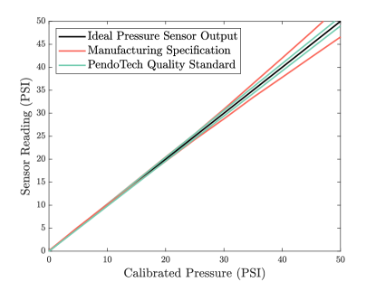
Figure 14: Technical specification for PendoTech pressure sensor.

The calibration of the PendoTech pressure sensor, illustrated in Figure 14, shows the ideal sensor response in black, the actual variation in response from testing a series of 100 sensors in red, and the quality standard for sensor performance in green. Sensors falling outside the green lines are not shipped to customers, determining the effective pressure resolution used throughout this study.

References

- Kim, Laschi, and Trimmer (2013) S. Kim, C. Laschi, and B. Trimmer, “Soft robotics: a bioinspired evolution in robotics,” Trends in biotechnology 31, 287–294 (2013).
- Majidi (2014) C. Majidi, “Soft robotics: a perspective—current trends and prospects for the future,” Soft robotics 1, 5–11 (2014).
- Roche et al. (2014) E. T. Roche, R. Wohlfarth, J. T. Overvelde, N. V. Vasilyev, F. A. Pigula, D. J. Mooney, K. Bertoldi, and C. J. Walsh, “A bioinspired soft actuated material,” Adv. Mater 26, 1200–1206 (2014).
- Harris, Elias, and Chung (2016) K. D. Harris, A. L. Elias, and H.-J. Chung, “Flexible electronics under strain: a review of mechanical characterization and durability enhancement strategies,” Journal of materials science 51, 2771–2805 (2016).
- Liu, Pharr, and Salvatore (2017) Y. Liu, M. Pharr, and G. A. Salvatore, “Lab-on-skin: a review of flexible and stretchable electronics for wearable health monitoring,” ACS nano 11, 9614–9635 (2017).
- Rogers, Someya, and Huang (2010) J. A. Rogers, T. Someya, and Y. Huang, “Materials and mechanics for stretchable electronics,” science 327, 1603–1607 (2010).
- Li et al. (2023) L. Li, L. Han, H. Hu, and R. Zhang, “A review on polymers and their composites for flexible electronics,” Materials Advances 4, 726–746 (2023).
- Ziaie et al. (2004) B. Ziaie, A. Baldi, M. Lei, Y. Gu, and R. A. Siegel, “Hard and soft micromachining for biomems: review of techniques and examples of applications in microfluidics and drug delivery,” Advanced drug delivery reviews 56, 145–172 (2004).
- Yeh et al. (2002) W.-C. Yeh, P.-C. Li, Y.-M. Jeng, H.-C. Hsu, P.-L. Kuo, M.-L. Li, P.-M. Yang, and P. H. Lee, “Elastic modulus measurements of human liver and correlation with pathology,” Ultrasound in medicine & biology 28, 467–474 (2002).
- Paszek et al. (2005) M. J. Paszek, N. Zahir, K. R. Johnson, J. N. Lakins, G. I. Rozenberg, A. Gefen, C. A. Reinhart-King, S. S. Margulies, M. Dembo, D. Boettiger, et al., “Tensional homeostasis and the malignant phenotype,” Cancer cell 8, 241–254 (2005).
- Samani and Plewes (2007) A. Samani and D. Plewes, “An inverse problem solution for measuring the elastic modulus of intact ex vivo breast tissue tumours,” Physics in Medicine & Biology 52, 1247 (2007).
- Last et al. (2011) J. A. Last, T. Pan, Y. Ding, C. M. Reilly, K. Keller, T. S. Acott, M. P. Fautsch, C. J. Murphy, and P. Russell, “Elastic modulus determination of normal and glaucomatous human trabecular meshwork,” Investigative ophthalmology & visual science 52, 2147–2152 (2011).
- Budday et al. (2015) S. Budday, R. Nay, R. De Rooij, P. Steinmann, T. Wyrobek, T. C. Ovaert, and E. Kuhl, “Mechanical properties of gray and white matter brain tissue by indentation,” Journal of the mechanical behavior of biomedical materials 46, 318–330 (2015).
- Finney (1967) E. Finney, “Dynamic elastic properties of some fruits during growth and development,” Journal of Agricultural Engineering Research 12, 249–256 (1967).
- Solomon and Jindal (2007) W. Solomon and V. Jindal, “Modeling changes in rheological properties of potatoes during storage under constant and variable conditions,” LWT-Food Science and Technology 40, 170–178 (2007).
- Engler et al. (2004) A. J. Engler, M. A. Griffin, S. Sen, C. G. Bonnemann, H. L. Sweeney, and D. E. Discher, “Myotubes differentiate optimally on substrates with tissue-like stiffness: pathological implications for soft or stiff microenvironments,” The Journal of cell biology 166, 877–887 (2004).
- Kong et al. (2005) H. J. Kong, J. Liu, K. Riddle, T. Matsumoto, K. Leach, and D. J. Mooney, “Non-viral gene delivery regulated by stiffness of cell adhesion substrates,” Nature materials 4, 460–464 (2005).
- Vedadghavami et al. (2017) A. Vedadghavami, F. Minooei, M. H. Mohammadi, S. Khetani, A. R. Kolahchi, S. Mashayekhan, and A. Sanati-Nezhad, “Manufacturing of hydrogel biomaterials with controlled mechanical properties for tissue engineering applications,” Acta biomaterialia 62, 42–63 (2017).
- Shopova et al. (2023) D. Shopova, A. Yaneva, D. Bakova, A. Mihaylova, P. Kasnakova, M. Hristozova, Y. Sbirkov, V. Sarafian, and M. Semerdzhieva, “(bio) printing in personalized medicine—opportunities and potential benefits,” Bioengineering 10, 287 (2023).
- Jammalamadaka and Tappa (2018) U. Jammalamadaka and K. Tappa, “Recent advances in biomaterials for 3d printing and tissue engineering,” Journal of functional biomaterials 9, 22 (2018).
- Murphy and Atala (2014) S. V. Murphy and A. Atala, “3d bioprinting of tissues and organs,” Nature biotechnology 32, 773–785 (2014).
- Radenkovic, Solouk, and Seifalian (2016) D. Radenkovic, A. Solouk, and A. Seifalian, “Personalized development of human organs using 3d printing technology,” Medical hypotheses 87, 30–33 (2016).
- Ye et al. (2015) E. Ye, P. L. Chee, A. Prasad, X. Fang, C. Owh, V. J. J. Yeo, and X. J. Loh, “Supramolecular soft biomaterials for biomedical applications,” In-Situ Gelling Polymers: For Biomedical Applications , 107–125 (2015).
- Patel and Gohil (2012) N. R. Patel and P. P. Gohil, “A review on biomaterials: scope, applications & human anatomy significance,” Int. J. Emerg. Technol. Adv. Eng 2, 91–101 (2012).
- Sharma et al. (2014) S. Sharma, D. Srivastava, S. Grover, and V. Sharma, “Biomaterials in tooth tissue engineering: a review,” Journal of clinical and diagnostic research: JCDR 8, 309 (2014).
- Nickerson et al. (2008) C. S. Nickerson, J. Park, J. A. Kornfield, and H. Karageozian, “Rheological properties of the vitreous and the role of hyaluronic acid,” Journal of biomechanics 41, 1840–1846 (2008).
- Zimberlin, McManus, and Crosby (2010) J. A. Zimberlin, J. J. McManus, and A. J. Crosby, “Cavitation rheology of the vitreous: mechanical properties of biological tissue,” Soft Matter 6, 3632–3635 (2010).
- Malone et al. (2018) F. Malone, E. McCarthy, P. Delassus, P. Fahy, J. Kennedy, A. Fagan, and L. Morris, “The mechanical characterisation of bovine embolus analogues under various loading conditions,” Cardiovascular engineering and technology 9, 489–502 (2018).
- Krasokha et al. (2010) N. Krasokha, W. Theisen, S. Reese, P. Mordasini, C. Brekenfeld, J. Gralla, J. Slotboom, G. Schrott, and H. Monstadt, “Mechanical properties of blood clots–a new test method,” Materialwissenschaft und Werkstofftechnik 41, 1019–1024 (2010).
- Balooch et al. (1998) M. Balooch, I.-C. Wu-Magidi, A. Balazs, A. Lundkvist, S. Marshall, G. Marshall, W. Siekhaus, and J. Kinney, “Viscoelastic properties of demineralized human dentin measured in water with atomic force microscope (afm)-based indentation,” Journal of Biomedical Materials Research: An Official Journal of The Society for Biomaterials, The Japanese Society for Biomaterials, and the Australian Society for Biomaterials 40, 539–544 (1998).
- Zheng and Mak (1999) Y. Zheng and A. Mak, “Extraction of quasi-linear viscoelastic parameters for lower limb soft tissues from manual indentation experiment,” (1999).
- Mahaffy et al. (2004) R. Mahaffy, S. Park, E. Gerde, J. Käs, and C.-K. Shih, “Quantitative analysis of the viscoelastic properties of thin regions of fibroblasts using atomic force microscopy,” Biophysical journal 86, 1777–1793 (2004).
- VanLandingham et al. (2005) M. R. VanLandingham, N.-K. Chang, P. Drzal, C. C. White, and S.-H. Chang, “Viscoelastic characterization of polymers using instrumented indentation. i. quasi-static testing,” Journal of Polymer Science Part B: Polymer Physics 43, 1794–1811 (2005).
- Hu et al. (2010) Y. Hu, X. Zhao, J. J. Vlassak, and Z. Suo, “Using indentation to characterize the poroelasticity of gels,” Applied Physics Letters 96 (2010).
- Lin et al. (2009) D. C. Lin, D. I. Shreiber, E. K. Dimitriadis, and F. Horkay, “Spherical indentation of soft matter beyond the hertzian regime: numerical and experimental validation of hyperelastic models,” Biomechanics and modeling in mechanobiology 8, 345–358 (2009).
- Style et al. (2013) R. W. Style, C. Hyland, R. Boltyanskiy, J. S. Wettlaufer, and E. R. Dufresne, “Surface tension and contact with soft elastic solids,” Nature communications 4, 2728 (2013).
- Raayai-Ardakani et al. (2019) S. Raayai-Ardakani, Z. Chen, D. R. Earl, and T. Cohen, “Volume-controlled cavity expansion for probing of local elastic properties in soft materials,” Soft matter 15, 381–392 (2019).
- Raayai-Ardakani, Earl, and Cohen (2019) S. Raayai-Ardakani, D. R. Earl, and T. Cohen, “The intimate relationship between cavitation and fracture,” Soft matter 15, 4999–5005 (2019).
- Gent and Lindley (1959) A. Gent and P. Lindley, “Internal rupture of bonded rubber cylinders in tension,” Proceedings of the Royal Society of London. Series A. Mathematical and Physical Sciences 249, 195–205 (1959).
- Ogden (1972) R. W. Ogden, “Large deformation isotropic elasticity–on the correlation of theory and experiment for incompressible rubberlike solids,” Proceedings of the Royal Society of London. A. Mathematical and Physical Sciences 326, 565–584 (1972).
- Chuong and Fung (1983) C. Chuong and Y. Fung, “Three-dimensional stress distribution in arteries,” (1983).
- Mijailovic et al. (2021) A. S. Mijailovic, S. Galarza, S. Raayai-Ardakani, N. P. Birch, J. D. Schiffman, A. J. Crosby, T. Cohen, S. R. Peyton, and K. J. Van Vliet, “Localized characterization of brain tissue mechanical properties by needle induced cavitation rheology and volume controlled cavity expansion,” Journal of the Mechanical Behavior of Biomedical Materials 114, 104168 (2021).
- Varner et al. (2023) H. Varner, G. P. Sugerman, M. K. Rausch, and T. Cohen, “Elasticity of whole blood clots measured via volume controlled cavity expansion,” Journal of the Mechanical Behavior of Biomedical Materials 143, 105901 (2023).
- Nafo and Al-Mayah (2021) W. Nafo and A. Al-Mayah, “Measuring the hyperelastic response of porcine liver tissues in-vitro using controlled cavitation rheology,” Experimental Mechanics 61, 445–458 (2021).
- Chockalingam et al. (2021) S. Chockalingam, C. Roth, T. Henzel, and T. Cohen, “Probing local nonlinear viscoelastic properties in soft materials,” Journal of the Mechanics and Physics of Solids 146, 104172 (2021).
- Mullins (1969) L. Mullins, “Softening of rubber by deformation,” Rubber chemistry and technology 42, 339–362 (1969).
- Delbos et al. (2012) A. Delbos, J. Cui, S. Fakhouri, and A. J. Crosby, “Cavity growth in a triblock copolymer polymer gel,” Soft Matter 8, 8204–8208 (2012).
- Fuentes-Caparrós et al. (2019) A. M. Fuentes-Caparrós, B. Dietrich, L. Thomson, C. Chauveau, and D. J. Adams, “Using cavitation rheology to understand dipeptide-based low molecular weight gels,” Soft Matter 15, 6340–6347 (2019).
- Chin et al. (2013) M. S. Chin, B. B. Freniere, S. Fakhouri, J. E. Harris, J. F. Lalikos, and A. J. Crosby, “Cavitation rheology as a potential method for in vivo assessment of skin biomechanics,” Plastic and reconstructive surgery 131, 303e–305e (2013).
- Polio et al. (2018) S. R. Polio, A. N. Kundu, C. E. Dougan, N. P. Birch, D. E. Aurian-Blajeni, J. D. Schiffman, A. J. Crosby, and S. R. Peyton, “Cross-platform mechanical characterization of lung tissue,” PloS one 13, e0204765 (2018).
- Cui et al. (2011) J. Cui, C. H. Lee, A. Delbos, J. J. McManus, and A. J. Crosby, “Cavitation rheology of the eye lens,” Soft Matter 7, 7827–7831 (2011).
- Zimberlin et al. (2007) J. A. Zimberlin, N. Sanabria-DeLong, G. N. Tew, and A. J. Crosby, “Cavitation rheology for soft materials,” Soft Matter 3, 763–767 (2007).
- Crosby and McManus (2011) A. J. Crosby and J. J. McManus, “Blowing bubbles to study living material,” Physics Today 64, 62–63 (2011).
- Zimberlin and Crosby (2010) J. A. Zimberlin and A. J. Crosby, “Water cavitation of hydrogels,” Journal of Polymer Science Part B: Polymer Physics 48, 1423–1427 (2010).
- Blumlein, Williams, and McManus (2017) A. Blumlein, N. Williams, and J. J. McManus, “The mechanical properties of individual cell spheroids,” Scientific reports 7, 7346 (2017).
- Kundu and Crosby (2009) S. Kundu and A. J. Crosby, “Cavitation and fracture behavior of polyacrylamide hydrogels,” Soft Matter 5, 3963–3968 (2009).
- ins (2024) “Materials testing systems - instron,” (2024), accessed: April 4, 2024.
- cohen-mechanics group (2024) cohen-mechanics group, “cots-benchtop-vcce,” https://github.com/cohen-mechanics-group/cots-benchtop-vcce (2024), accessed: April 15, 2024.
- Zumba, Zumba, and Zumba (2023) G. G. Zumba, J. G. Zumba, and H. G. Zumba, “The contribution of the physical space in medical space,” Human Factors in Architecture, Sustainable Urban Planning and Infrastructure 89 (2023).
- RAWLINSON (1978) C. RAWLINSON, “Space utilization in hospitals,” Journal of Architectural Research , 4–12 (1978).
- Tung et al. (2018) M. Tung, R. Sharma, J. S. Hinson, S. Nothelle, J. Pannikottu, and J. B. Segal, “Factors associated with imaging overuse in the emergency department: a systematic review,” The American journal of emergency medicine 36, 301–309 (2018).
- Marin and Mills (2015) J. R. Marin and A. M. Mills, “Developing a research agenda to optimize diagnostic imaging in the emergency department: An executive summary of the 2015: Academic emergency medicine: Consensus conference,” Pediatric Emergency Care 31, 876–882 (2015).
- Roth (2020) C. B. Roth, Local Probing and Modelling of Viscoelasticity in Soft Materials, Masterthesis, Ecole Polytechnique Fédérale de Lausanne, Lausanne, Switzerland (2020), advanced Volume Controlled Cavity Expansion, Mechanical Engineering.
- Love (1888) A. E. H. Love, “Xvi. the small free vibrations and deformation of a thin elastic shell,” Philosophical Transactions of the Royal Society of London.(A.) , 491–546 (1888).
- Fukada, Fang, and Shigeno (2011) S. Fukada, B. Fang, and A. Shigeno, “Experimental analysis and simulation of nonlinear microscopic behavior of ball screw mechanism for ultra-precision positioning,” Precision Engineering 35, 650–668 (2011).
- Saruhan et al. (2014) H. Saruhan, S. Saridemir, A. Qicek, and I. Uygur, “Vibration analysis of rolling element bearings defects,” Journal of applied research and technology 12, 384–395 (2014).
- Hoffmann (1974) K. Hoffmann, Applying the wheatstone bridge circuit (HBM Darmstadt, Germany, 1974).