Quantum study of the CH photodissociation in full dimension Neural Networks potential energy surfaces
Abstract
CH, a cornerstone intermediate in interstellar chemistry, has recently been detected for the first time by the James Webb Space Telescope. The photodissociation of this ion is studied here. Accurate explicitly correlated multi-reference configuration interaction ab initio calculations are done, and full dimensional potential energy surfaces are developed for the three lower electronic states, with a fundamental invariant neural network method. The photodissociation cross section is calculated using a full dimensional quantum wave packet method, in heliocentric Radau coordinates. The wave packet is represented in angular and radial grids allowing to reduce the number of points physically accessible, requiring to push up the spurious states appearing when evaluating the angular kinetic terms, through a projection technique. The photodissociation spectra, when employed in astrochemical models to simulate the conditions of the Orion Bar, results in a lesser destruction of CH compared to that obtained when utilizing the recommended values in the kinetic database for astrochemistry (KIDA).
I Introduction
The long-sought-after CH cation has been recently detected for the first time in a protoplanetary disk (d203-506) illuminated by the strong far ultraviolet (FUV) radiation field from nearby massive stars in Orion’s Trapezium cluster Berné et al. (2023). This detection was only possible in the infrared, through vibrational spectroscopy, at 1400 cm-1, within the PDRs4All program using the James Webb Space Telescope (JWST). This highly symmetric cation, with a planar configuration, has no permanent dipole moment and thus cannot be observed through microwave rotational spectroscopy. On the contrary, the rotational spectra of its deuterated isotopologues, such as CH2D+ or CHD, has been experimentally characterized Gärtner et al. (2013); Jusko et al. (2017); Töpfer et al. (2018), but only a tentative detection of CH2D+ has been reported so far Roueff et al. (2013).
Hydrides are the first molecules to form in the interstellar medium (ISM) and provide crucial information on the physical conditions, such as the cosmic-ray ionization rate and H2/H abundance ratios Gerin et al. (2016). The precise determination of their abundances is key to the following chemistry in the ISM. Carbon hydrides are of paramount importance because the allotropy of carbon triggers the molecular complexity in space: from organic and prebiotic molecules, to polycyclic aromatic hydrocarbons (PAH’s), amorphous carbon and many different minerals. CH cations are particularly important because ion-molecule reactions are typically faster and the low ionization energy of carbon (11.3 eV), below that of hydrogen (13.6 eV), produces high C+/C abundance ratios in molecular gas irradiated by FUV (6 eV E 13.6 eV). Carbon cations present very anomalous properties, giving rise to the development of the field of the carbocation chemistryPrakash and v. R. Schleyer (1997); Olah and Orakash (2004), where the spectroscopic characterization of these species, pioneered by Takeshi Oka Crofton et al. (1988); Jagod et al. (1992); White et al. (1999); Wang et al. (2013), plays an important role not only in astrochemistry but also in combustion chemistry.
The smallest CH+ carbocation is formed in C + H or C+ + H2 reactions. The reaction C+ + H2 is endothermic by 0.5 eV Gerlich et al. (1987), but it becomes exothermic for vibrationally excited H Hierl et al. (1997). It is known that enhanced abundances of FUV-pumped vibrationally excited H2 significantly increase the reactivity of H2 in FUV-irradiated molecular cloudsA. G. G. M. Tielens and D. Hollenbach (1985); Sternberg and Dalgarno (1995); Agúndez et al. (2010), so-called photodissociation regions (PDRs). Indeed, observations of PDRs reveal the presence of vibrationally excited H2 up to in several interstellar PDR’sKaplan et al. (2017, 2021). The use of quantum state-to-state rate constants in chemical formation and excitation models applied to the formation of CH+ describes very well the observed rotational emission lines detected in PDRs Zanchet et al. (2013); Faure et al. (2017).
Once CH+ is formed, the successive addition of hydrogen atoms occurs via reactive collisions with H2, in exothermic or nearly thermoneutral reactions of the type H2 + CH H + CH. This sequence stops at CH, because the reaction H2 + CH is very slow and no CH products are observed in several experimentsSmith et al. (1982); Asvanay et al. (2004); Asvany et al. (2018). The reaction to form the floppy methane cation R. Signorell and F. Merkt (1999); Wörner et al. (2006), CH, is endothermic and is not expected to be formed in this hydrogenation sequence. Instead, CH is probably formed from neutral CH4 by photoionization or electron impact, and this cation can react again with H2 to form CH Asvany et al. (2004), a very floppy cation whose infrared spectra have been widely studiedSchreiner et al. (1993); White et al. (1999); Asvany et al. (2015).
The relative stability of CH with H2 makes this cation play an important role in the formation of more complex molecules Dalgarno (1985); Wakelam et al. (2010); Chabot et al. (2020). The deuteration of CH is relatively fast Smith et al. (1982); Asvanay et al. (2004); Asvany et al. (2018) and its deuterated isotopologues are considered to be determinant in the gas phase formation of complex deuterated molecules, whose observed abundance is several orders of magnitude higher than expected based on the cosmic D/H ratio. Moreover, since the rovibrational spectra of CH can be observed by JWST, CH is expected to be a useful diagnostic to determine the physical conditions of FUV-irradiated environments (from clouds to protoplanetary disksBerné et al. (2023); Henning et al. (2024)).
The vibrational spectroscopy of CH has been the subject of many theoretical Kraemer and Spirko (1991); Yu and Sears (2002); Nyman and Yu (2019); Changala, P. B. et al. (2023) and experimental Crofton et al. (1985, 1988); Jagod et al. (1992); Asvany et al. (2018) studies. The photoionization of the neutral methyl radical has also been studied using several techniques Blush et al. (1993); Wiedmann et al. (1994); Liu et al. (2001); Schulenburg et al. (2006); Taatjes et al. (2008); Loison (2010); B. K. Cunha de Miranda and C. Alcaraz and M. Elhanine and B. Noller and P. Hemberger and I. Fischer and G. A. Garcia and H. Soldi-Lose⊥ and B. Gans and L. A. Vieira Mendes and S. Boyé-Péronne and S. Douin and J. Zabka and P. Botschwina (2010); B. Gans and L. A. Vieira Mendes and S. Boyé-Pérone and S. Douin and G. García and H. Soldi-Lose and B. Cunha de Miranda anid C. Alcaraz and N. Carrasco and P. Pernot and D. Gauyacq (2010); Changala, P. B. et al. (2023), which also gives information of the rovibrational structure of the CH cation.
The photodissociation cross sections of CH+, CH and CH have been reported previously Heays et al. (2017). However, there is only one study on the photodissociation of CH carried out nearly 50 years ago Blint et al. (1976), in which vertical excitation was considered from the planar equilibrium geometry on the ground electronic state. It was concluded that the oscillator strength leading to dissociation from the ground electronic state is very low. It is worth mentioning that, in the kinetic data base for astrochemistry (KIDA), the recommended rate constant for the photodissociation of CH under the local mean interstellar radiation field is s-1 (see also Ref. Tielens (2010)). The value of s-1 is rather high according to the previous study Blint et al. (1976), and it is therefore important to determine the photodissociation rate of CH more accurately.
The objective of this work is to study the photodissociation cross-section of CH using quantum full dimension dynamics to properly assess the destruction of this cation under different FUV radiation fields. The work is distributted as follows. In section II the ab initio calculations of the first electronic states of CH are described. The neural network fitting of the first three electronic states are described in section III. The vibrational bound states of the ground electronic states are described in section IV. The transition dipole moments and their fit are described in section V. The calculation of the photodissociation cross section are described in section VI, and their use in astrochemical models in section VII. Finally, section VIII is devoted to extract some conclusions.
II Electronic states
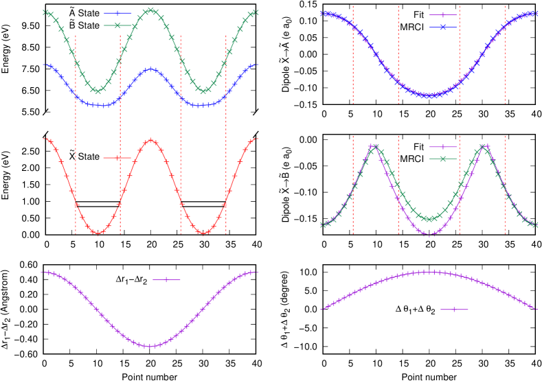
The three lower electronic states of CH are calculated using the explicitly correlated internally contracted multi-reference configuration interaction (ic-MRCI-F12) method Werner and Knowles (1988); Shiozaki and Werner (2011), with the MOLPRO suite of programs Werner et al. (2012) and the cc-pCVTZ-F12 electronic basis setHill et al. (2010). The molecular orbitals are optimized using the state-averaged complete active space self-consistent field (SA-CASSCF) method, with 7 active orbitals, for the three lower singlet electronic states. Hereafter, the origin of energy is set at the planar equilibrium configuration of the ground state, with a C–H distance of 1.0892 Å, in very good agreement with previous calculations Blint et al. (1976); Kraemer and Spirko (1991); Yu and Sears (2002); Delsaut (2015). An energy diagram of the three first electronic states is shown in Fig. 1.
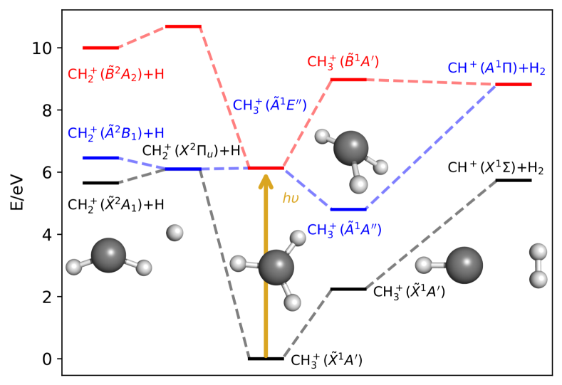
The ground electronic state correlates adiabatically with the CH() + H and CH+() + H2 asymptotes, which are both located at 6 eV over the equilibrium configuration. The ground and first excited electronic states tend to the linear CH() + H fragments, presenting a Renner-Teller interaction. The path towards the formation of CH+ + H2 can be seen as a subsequent step after the formation of CH + H, where the H approaches one of the CH’s hydrogens, which is in an almost linear configuration. The C–H bond breaks while the H–H forms towards the CH++H2 geometry. Due to the proximity of these geometries to the CH linear configuration, the process occurs close to a conical intersection (CI). The first adiabatic excited electronic states does not lead to CH+ in the ground state but in the excited , a degenerate state towards which the second excited state also correlates.
Considering a vertical excitation, the first electronic state corresponds to the double degenerate , at the highly symmetric geometry of the ground equilibrium geometry, as reported previously Blint et al. (1976); Delsaut (2015). The next excited states in the Franck-Condon region, the and , are 13 eV higher, close to the atomic hydrogen ionization and are not expected to contribute significantly.
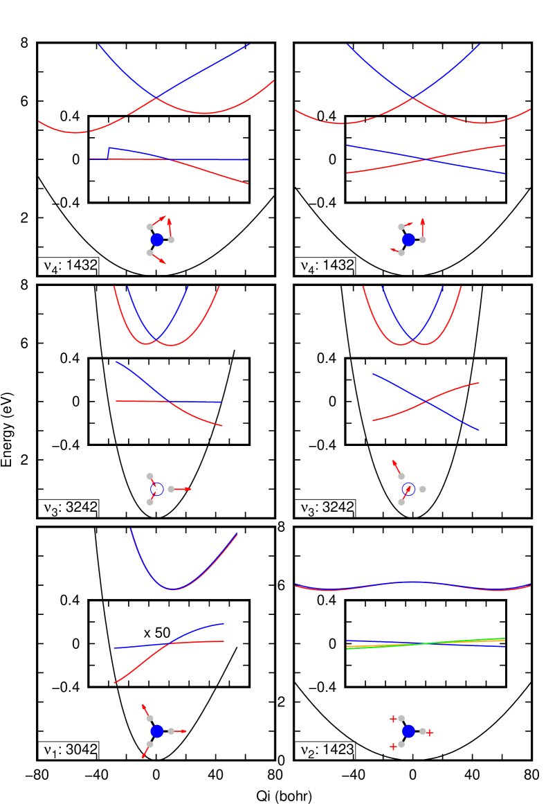
The cuts of the potential along the normal coordinates of the ground state are shown in Fig. 2. These normal modes are in good agreement with previously reported ones Blint et al. (1976); Delsaut (2015) and correspond to the singly degenerate states, , the symmetric stretching, and , the umbrella vibration, and two degenerate vibrations, and . The elongation of the normal coordinates for and remains in the and symmetry, respectively, and the two excited electronic states remain degenerate. This degeneracy is broken along the degenerate vibrations, and , showing the typical CI behavior of the Jahn-Teller effect, with the seam at the configuration of highest symmetry.
III Neural network potential energy sufaces fitting
New analytical full dimensional potential energy surfaces (PESs) have been developed to describe the three lower adiabatic electronic states of CH. A fundamental invariant neural network (FI–NN)Shao et al. (2016) takes into account the exact permutation symmetry of the three hydrogen atoms. Three FI–NN are trained –one for each of the three adiabatic energies. While a single FI–NN could handle the calculation of the three electronic states, this setup provides more flexibility in order to make use of the most accurate PESs for different tasks: vibrational state calculation in the ground electronic state and quantum dynamics in the excited states. Moreover, the data from the third excited state tends to be noisier due to interactions with higher excited states, what could interfere with the training process.
In all cases, the multilayer perceptron (MLP) architecture is used, which involves two hidden layers with 50 neurons each. Hyperbolic tangents are used as activations between the hidden layers. The input features are represented by fundamental invariants (FI) of the functions, with and the interatomic distance between atoms and . There is a total of nine FI for the A3B case, which expressions are provided elsewhere FId . The mathematical expression of the MLPs is the standard one, where the values of the th neuron in the layer are computed through those from the previous layer and a trainable set of weights () and bias (). represents the activation function —the hyperbolic tangent or linear function.
| (1) |
The MLPs are trained on a set of nearly 25000 energies computed at a ic-MRCI-F12/cc-pCVTZ-F12 level of theory with MOLPRO 2012. An extra set of about 5000 energies is left as test set. A total of ten models are trained, but only the one which better performs on the test set is used. Building this energy dataset is performed in an iterative process, which starts with a rather small set of geometries computed from normal mode displacements of equilibrium geometries and then includes data from minimum energy paths or quantum and classical dynamics on intermediate fits of the system. These fits are done up to 15 eV and 25 eV for the two first and third electronic states, respectively.
The training process is similar to those previously described for H and OH + H2CO systems del Mazo-Sevillano et al. (2021, 2023) and is performed with an in-house Python code based on PyTorch libraryPaszke et al. (2019). An L-BFGS optimizerLiu and Nocedal (1989) is used and the loss function is the Mean Square Error (MSE) error of the predicted energies compared with the ic-MRCI-F12/cc-pCVTZ-F12 energies:
| (2) |
where is the total amount of training data and is the th energy. The asterisk indicates ab initio energy.
The Root Mean Square Error (RMSE) of the three PES is presented in table 1 for several energy ranges. The errors are shown in meV units. The PES for the state remains accurate up to electronic energies of 6–7 eV, enough to compute highly accurate vibrational states. The PESs for the and states remain accurate up to higher electronic energies, although the latter presents larger errors, in part due to the difficulty to converge the ab initio calculations for this state, which interacts with higher excited electronic states.
| E /eV | State | State | State |
|---|---|---|---|
| – | – | ||
| – | |||
In the following we analyse in more detail the and states. Fig. 3 presents the relaxed PES over two radial coordinates and , using heliocentric Radau coordinates as defined below. For the state there is a minimum, corresponding to a CH (). The minimum in the state is in the Franck–Condon region and corresponds to CH ().
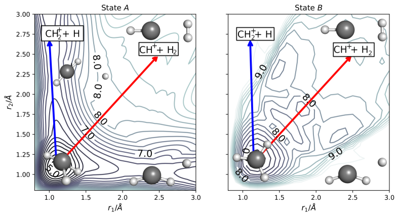
The path to the CH + H product occurs in the state after surpassing a low energy transition state less than 1 eV above the minimum. On the other hand, the path to the CH+ + H2 is highly endothermic, eV over the minimum, with no barrier. The path towards the formation of CH + H can be merely explain as a C–H elongation —related to the elongation of the coordinate in Fig 3. The path towards CH+ + H2 is not so direct, and proceeds via elongation of one of the C–H distances getting close to a CH configuration. After this, the second distance elongates breaking a C–H bond while forming the H2 molecule. In both cases the minimum energy paths get close to an almost linear configuration of the CH —a state, degenerate with the ground electronic state— what implies that and electronic states get close in energy as the photodissociation process occurs.
Regarding the reactions on the state we find that both reactions are highly endothermic. The Franck–Condon region becomes the absolute minimum with no other product close in energy as the CH + H in the electronic state. Hence, we do not expect reactivity in this state to be important up to photon energies eV and eV for CH+ + H2 and CH + H respectively. For this reason, we expect the CH in the electronic state to remain mostly bounded for the photon energies of interest in this work.
IV Bound vibrational states
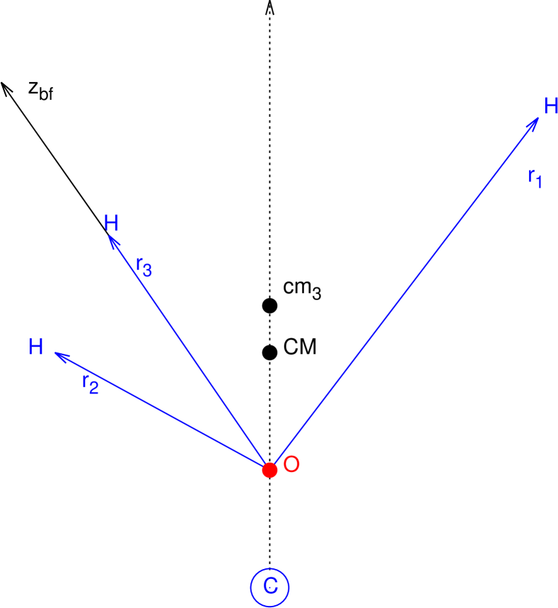
The bound state calculations are done in two steps: first, the eigenvalues are calculated using an iterative non-orthogonal Lanczos methodCullum and Willoughby (1985), and second, a conjugate gradient methodFröberg (1985); Wyatt (1989) is used to obtain the eigenvectors. These procedures are implemented in a parallel MPI form using heliocentric Radau coordinates Smith (1980); Yu and Muckerman (2002); Yu and Sears (2002), illustrated in Fig. 4. Three vectors are defined, corresponding to the distance of each hydrogen to a center O, situated along the line joining the centers-of-mass of CH and H3. This center O is chosen to make zero the kinetic coupling terms among the vectors , and the Hamiltonian thus built is formally identical to that of Jacobi coordinatesSmith (1980); Yu and Muckerman (2002). A body-fixed frame is chosen, in which lies parallel to the -axis, and is in the body-fixed plane. Thus the coordinates are separated as three external Euler angles, , defining the body-fixed frame, and six internal coordinates , and . The wave functions, for a given total angular momentum , are described as
where are Wigner rotation matrices Zare (1988), with and being the projections of the total angular momentum on the space-fixed and body-fixed frames respectively.
The internal coordinates are described in grids. Sinc Discrete Variable Representation (DVR) Colbert and Miller (1992) is used to describe the radial coordinates, non-orthogonal Gauss-Legendre DVR Corey and Lemoine (1992); Corey et al. (1993) to describe , and equispaced points in the interval to describe . The evaluation of each kinetic term is done by transforming to finite basis representation (FBR), where it is analytical. This transformation is done sequentially, one internal coordinate by one, to save computation time as it is done in other approaches representing the wave function in the FBR and then transforming sequentially to the DVR to evaluate the potentialGoldfield (2000); Lin and Guo (2002).
Representing the wave functions in grids for internal coordinates has the advantage of saving many points, the so called L-shaped gridsMowrey (1991), thus reducing considerably the memory and time requirements of the calculations. However, the numerical sequential method done to transform from DVR to FBR, usually introduces spurious states when evaluating the rotational kinetic terms using finite DVR grid points. To avoid this problem, we have developed a projection method to move the spurious states up, out of the physical energy interval of interest, as described in the appendix.
The bound state calculations are done using a grid of 20 DVR points in the radial coordinates, , in the interval Å, 30 Gauss-Legendre points for , and 61 points in . About 104 Lanczos iterations were done to converge the eigenvalues.
Fig. 5 shows the cuts of the density probability associated to some bound states; those corresponding to the ground and first excitation on each mode (, , , ) for total angular momentum . Their energies are tabulated in Table. 2. The heliocentric Radau coordinates are well adapted to describe the permutation symmetry of the hydrogen atoms, but in this first implementation no symmetry–adapted basis functions or grids are used. For the degenerate modes ( and ) only one case is shown.
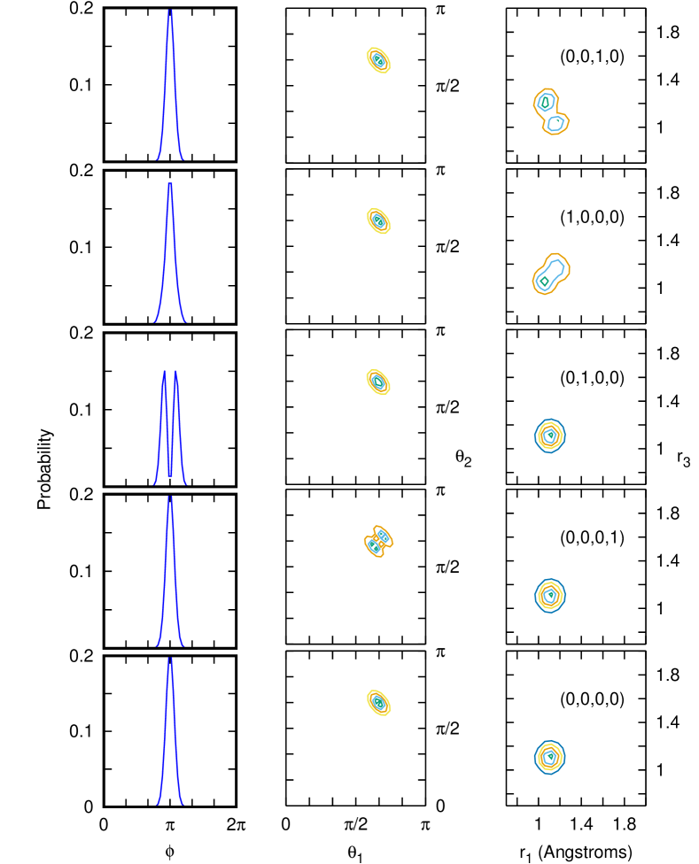
| vibrational mode | This work | Ref.Kraemer and Spirko (1991) | Ref.Changala, P. B. et al. (2023) |
|---|---|---|---|
| 2947.82 | 2949.8 | 2943.43 | |
| 1424.53 | 1432.5 | 1405.72 | |
| 3113.50 | 3091.3 | 3109.06 | |
| 1393.91 | 1399.3 | 1394.98 |
The lowest eigenvalues for each vibrational mode corresponding to the bound states in the ground electronic state are listed in Table 2, together with other theoretical values for comparison. The values of Ref. Changala, P. B. et al. (2023) were obtained to simulate the rovibrational spectra observed in the d203-506 protoplanetary disk and experimental data. The present results are within 5 cm-1 accurate with respect to those previously reported Kraemer and Spirko (1991); Yu and Sears (2002); Changala, P. B. et al. (2023), except for the mode, which deviates 20 cm-1. Previous calculations are based on local fits for the potential, thus describing only the bound states. In this work, however, the potential energy surfaces are global, , they are built to describe the bound states and the fragmentation regions towards the CH+ + H2 and the CH + H products. For these reasons, we consider this new PES as accurate enough to describe the photodissociation dynamics, with nearly spectroscopic accuracy.
V Transition dipole moments
The transition dipole moments required for the and electronic excitation are calculated with MOLPRO programs Werner et al. (2012), and to avoid the randomness of the phase of adiabatic eigenvectors, a biorthogonal transformation is used between consecutive points along lines. The Cartesian projections of the transition dipole moments are also shown, in the boxed inset in Fig. 2, for the and excitations, with the molecule being in the plane for the equilibrium geometry. In all cases, the transition dipole moments are zero at , corresponding to the equilibrium geometry. Only corresponds to a motion out of the plane of the planar geometry, and it is the only one to have non zero components in , and axis. For the rest of the normal modes, only the component , perpendicular to the plane of the molecule, is non-zero. This transition dipole moment corresponds to a transition between two of the bonding orbitals of the C+ atom (mostly corresponding to a hybridization) to an unoccupied orbital, out of the plane Delsaut (2015). As a consequence of the CI of the and excited states in geometriesGuan et al. (2020), there is a sign change of the real electronic part of the wave function under a 2 rotation in the vibrational coordinates, a special case of Berry’s geometrical phase.Herzberg and Longuet-Higgins (1963); Berry (1984); Xie et al. (2017)
The three components of both transition dipole moments have been fitted to an analytical function, based on mono–dimensional grids for each internal heliocentric Radau coordinates. The fits are localized in the CH () well, switching to zero outside this region. There is no general method for an accurate representation of the dipole moment for polyatomic molecules, using an appropriate functional form. Because the dipole moment is a vector property, its fit is more complicated than that for the energiesGuan et al. (2020). One alternative is to use a diabatic representation where the dipole moment is diagonal. In this work we are interested in fitting the adiabatic transition dipole moments between the ground electronic state and the excited and () states.
The phase of the adiabatic transition dipole moment is arbitrary, because it depends on the phase of the electronic wavefunctions and . In addition, the adiabatic representation becomes inadequate near CIs Guan et al. (2020), because real-valued adiabatic electronic wavefunction changes sign when transported around a CI (geometric or Berry phase)Berry (1984); Xie et al. (2017). In order to make the transition dipole moment continuous, we have calculated the overlap of each electronic state with the same electronic state at a reference geometry –the equilibrium geometry of the ground electronic state– using the biorthogonalization method as programmed in MOLPRO programWerner et al. (2012). The signs of and are corrected in order to make the overlap positive, and then corrects the phase of . Therefore, in the adiabatic approximation we have not taken into account this change of sign of real electronic wave functions that produces a change of sign of the transition dipole moment when the conical intersection is surrounded in nuclear configuration space.
Once corrected the sign, in order to fit the transition dipole moment, we have expanded each component of the dipole moment as a function of symmetry coordinates of the point group, defined in terms of the Heliocentric Radau coordinates defined above as
being and the variation with respect to equilibrium values, Å and and where is selected as the out-of-plane variation of the Radau angle with respect to the equilibrium value, .
As shown in Fig. 2, the stretching mode corresponds to the variation of the symmetry coordinate, that belongs to the irrep of the point group. As a consequence, the only non-zero component is the out-of-plane component, although in this case it is practically zero, and can be discarded. The bending mode corresponds to the variation of the out-of-plane coordinate. This mode belongs to the irrep of the point group. In this case the non-zero components are the component for the transition and the component for the transition. The other modes are degenerated, and corresponds to the irrep. corresponds to stretching modes, which can be described by and , while correspond to bending modes that are described by and . In this cases the non-zero component of the transition dipole is the component.
Since the ( ) coordinates do not take into account the symmetry properties of the dipole moment with respect to the exchange of two hydrogens, they are antisymmetrized as
where is the permutation operator for atoms and and where is a phase to take into account the symmetry of each component with respect to permutation of two hydrogens. When the dipole is antisymmetric with respect to the permutation, is obtained as the sign of the maximum value of or . Finally, each Cartesian component of the transition dipole moment for the transition from to states is expanded as a series in this symmetry coordinates
with in this case and where are also developed as a serie
where is the degree of the polynomial, and where the expansion has been multiplied by a Gaussian function in order to avoid extremely large values of the dipole moment in regions very far from the equilibrium position.
In Fig. 6 we show the variation of the transition dipole moment when the symmetry coordinates and are varied simultaneously, following a sinusoidal movement.
VI Photodissociation cross section
The photodissociation cross section is calculated for each transition with a wave packet method, using the heliocentric Radau coordinate, as described above for the bound state calculations. The modified Chebyshev propagator Mandelshtam and Taylor (1995); Chen and Guo (1996); Gray and Balint-Kurti (1998); González-Lezana et al. (2005) is used to integrate the Schrödinger equation as
| (4) | |||||
where is the scaled Hamiltonian, with and , and being the minimum and maximum energy values of the Hamiltonian of the system represented in the grid/basis using in the propagation. The wave packet at time and eigenfunctions at energy are expressed in terms of the Chebyshev iterations, , as
| (5) |
with
| (6) | |||||
with being a Bessel function of the first kind.
The absorption cross section is then given by
with and denoting the real part. For finite propagations (in this case 1000 Chebyshev iterations), the right–hand side of Eq. VI is multiplied by , with in the present case.
The wave packet is represented in grids for the internal radial and angular coordinates, using the projection method to shift up the spurious solutions described in the appendix. The angular grids are those used for bound states, while the radial grids are extended to 50 points, keeping the same density of points. The initial wave packet is built for the =0 =1 transition as described previouslyPaniagua et al. (1999); Aguado et al. (2003); Chenel et al. (2016), combining the bound state with the transition dipole moment to the final electronic states, or , and projecting on a final . This is done for several bound states with different values. The wave packet is propagated about 1000 iterations. At each iteration the autocorrelation function is evaluated, and photoabsorption cross section is obtained by a Chebyshev transformation to the energy domain González-Lezana et al. (2005).
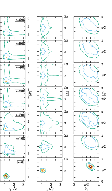
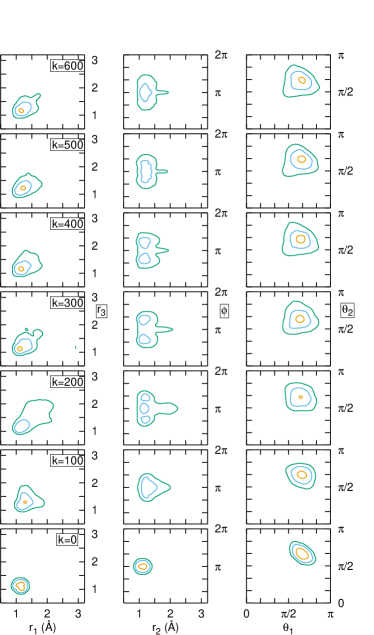
In Fig. 7, contour plots of the density probability of the wave packet component, , are shown for the (left panels) and (right panels) transitions, for several values of
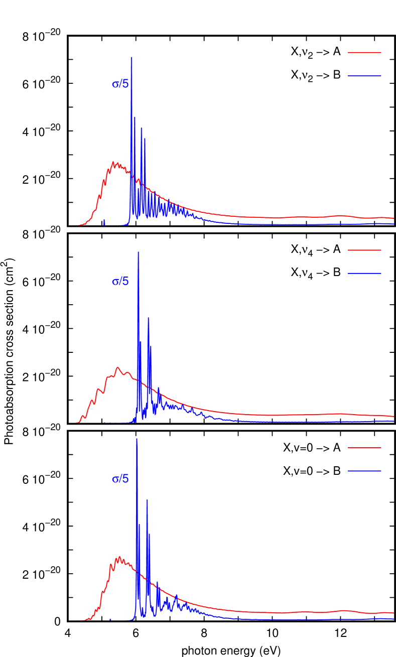
The photoabsorption cross section towards the and electronic states are shown in Fig. 8 for different initial vibrational states. To explain the differences between absorption to and states, it is important to remind that they present a conical intersection at the Franck-Condon region. Thus, the state corresponds to a local maximum which tends rapidly to the dissociation limits. One of these limits corresponds to the CH + H products, slightly below the vertical excitation. On the other side, towards the CH + H2 products there is an avoided crossing between the and state, from which the potential energy increases monotonically towards the CH + H2 asymptote, at 8.68 eV. The absorption spectrum shows a broad band characteristic of a direct dissociation, mostly below photon energies of 8 eV (corresponding to total energies of 8.84 eV). Clearly, the dissociation must be towards the lower CH + H products, which is also supported by the inspection of the wave packet dynamics and the PESs. The absorption band shows some weak peaks at the lower energies associated to resonances originated by the well around the minimum CH in Fig. 1, which are above the CH + H dissociation limit.
The upper part of the conical intersection, the state, corresponds to a well, showing dissociation limits at 10.6 eV (CH + H) and 8.68 eV (CH + H). Moreover, the PES shows a barrier of 10 eV when elongating one distance towards the CH + H products. As a consequence the absorption corresponds to resonant bound–bound transitions, with the wave packet oscillating around the Franck-Condon regions showing many recurrences, mostly at photon energies below 9 eV ( at total energies of 9.84 eV). Above this energy, the system can dissociate in the adiabatic state, what occurs with a low probability. Therefore, most of the wave packet should dissociate by tunnelling at the CI, which tends mainly towards the CH + H products.
The spectra of vibrationally excited CH(, =4,2) shows very similar patterns. The bands for all vibrational states considered are very close, with a shift in the photon energy of 1400 cm-1 (0.174 eV) between the ground and the two excited vibrational states. The spectrum for shows a different intensity pattern as compared to that of the ground vibrational, as a result of the excitation on the angles. However, the for gets closer to that of the ground, what is explained by the shallower dependence of the potential on the out-of-plane angle .
VII Astrochemical modeling
The photodestruction of CH in strongly FUV-irradiated objects (such as interstellar PDRs and protoplanetary disks) is determined by the photodissociation rate, , the integral of the photodissociation cross section with energy dependent FUV radiation field. Using Draine’s Draine (1978) mean interstellar radiation field, the CH photodissociation rate is s-1, 7.24 s-1 and 7.13 s-1 for the ground vibrational state ( in Fig. 8), and for the and excited vibrational states, respectively, with a very minor increase with vibrational excitation of 5-7 . These values are about 300 times lower than the value of s-1 recommended in KIDA data base. Moreover, KIDA suggests that two photodestruction products, CH and CH+, form at the same rate, while according to this work the only product is CH + H.
The photodissociation rate calculated here is rather low, in agreement with the previous estimation by Blint and co-workers Blint et al. (1976). The values reported for CH+, CH and CH are , and 2 s-1, respectivelyHeays et al. (2017). These rates are higher than those obtained here for CH by a factor of 30. The reason for this is attributed to the “forbidden” nature of the transition dipole moment of CH at the equilibrium configuration.
In interstellar clouds strongly illuminated by FUV photons, photoionization of carbon atoms produces a high abundance of electrons, which rapidly recombine with cations, producing excited neutral systems that dissociate. This dissociative recombination (DR) process is very fast, because of the strong Coulomb interactions, of the order of 10-7 s-1. Because of the large difference between the photodissociation and DR rates (of about 4 orders of magnitude), it is expected that the destruction of CH is dominated by electrons and not by photons.
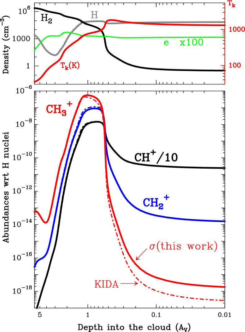
To show the effect of the photodissociation cross section obtained in this work, and the competition with other processes, Fig. 9 shows an example obtained with the Meudon PDR model Le Petit et al. (2006); Goicoechea and Le Bourlot (2007) of a strongly FUV-irradiated molecular cloud, with a FUV radiation field times the mean interstellar radiation field in the solar neighbourhood, and a constant thermal pressure K cm-3. These parameters are appropriate to the Orion Bar PDR, an irradiated rim of the Orion molecular cloudGoicoechea et al. (2016). The upper panel of Fig. 9 shows the predicted gas density, electron density, and temperature profile as a function of depth into the molecular cloud (in magnitudes of visual extinction, AV). The lower panel shows the resulting abundance profiles, with respect to H nuclei, for the main species discussed in the text. The continuous curves refer to a model that integrates the wavelength-dependent CH photodissociation cross-sections determined in this work for the A and B electronic states and leading to CH as products. The dashed curve shows a model that uses the CH photodissociation rate recommended in KIDA. The dominant process destroying CH is dissociative recombination with electrons, thus the two models predict relatively similar abundance profiles. The role of CH photodissociation is more clearly seen at the very edge of the PDR, at low AV, where the flux and energy of FUV photons is high. Here, the model using the recommended rate in KIDA is not realistic and underestimates the CH abundance by a factor of about 6. Such difference explains the need of realistic evaluations of the rate constants used in the astrochemical models.
VIII Conclusions
A quantum treatment is developed to study the photodissociation of the CH cation below 13.6 eV. Accurate full dimension PESs are generated using a FI-NN method for the three lower electronic states based on ic-MRCI-F12/cc-pCVTZ-F12 ab initio. The transition dipole moments are also fit locally in the region around the equilibrium configuration covering the vibrational bound states in the ground electronic state.
The bound states and wave packet dynamics are studied using heliocentric Radau coordinates, well adapted to account for the permutation symmetry of the three hydrogen atoms. A full grid representation of the internal (radial and angular) coordinates is implemented, allowing saving of memory and computation time due to the L-shape method that allow to discard the grid points with high energy out of the energy range of physical interest. To do so, it was found necessary to apply a projection method to push up the spurious states appearing when evaluating the angular kinetic terms using a sequential transformation from a non-direct DVR basis set to the FBR representation. This is implemented in the home made MadWave4 code, a MPI parallel code written in Fortran.
The calculated bound eigenvalues in the ground electronic states are in good agreement with previous theoretical and experimental ones. The photodissociation cross section from several initial vibrational states towards the excited and electronic states have been calculated using a quantum wave packet method. The initial vibrational excitation has little influence in the photodissociation dynamics and the calculated photodissociation rate is about 300 times lower than the recommended one in the KIDA data base for astrochemistry.
The possible fragmentation products in the adiabatic representation is mostly towards the CH+ H products for the state. On the electronic state, however, most of the absorption spectrum corresponds to the bound region, and without including non-adiabatic transitions the wave packet cannot yield to dissociation. It is considered that this bound wave packet could be trasferred to the state, where it can dissociate. A diabatization of the electronic Hamiltonian is being done to consider the non-adiabatic transitions needed to a proper description of the branching ratios. This is left for a future work
The effect of the calculated cross section in interstellar regions strongly illuminated by FUV photons is analyzed using the Meudon PDR code applied to the Orion Bar as a prototype. It is found that the dominant destruction mechanism of CH is the dissociative recombination with electrons, and that the use of the KIDA photodissociation rate underestimates the CH abundance, demonstrating the need of realistic evaluation of rate constants in astrochemical models.
IX Supplementary Material
The three Neural Network PESs, in fortran programs, and the photodissociation cross section obtained for the ground vibrational state obtained in this work are supplied in the Supplementary information, giving detailed information about how to be used.
X Acknowledgements
The research leading to these results has received funding from MICIN (Spain) under grants PID2021-122549NB-C21, PID2021-122549NB-C22 and PID2019-106110GB-I00. We thank the PDRs4All-JWST-ERS team for their work in planning, obtaining, and calibrating the spectroscopic observations that led to the detection of interstellar CH.
XI Data availability Statement
The data that support the findings of this study are available from the corresponding author upon reasonable request.
Appendix A Projecting up spurious solutions
We describe here a method to eliminate spurious states that appear when using fdiscrete variable representation (DVR) and a sequential transformation to the finite basis representation (FBR) to evaluate the angular kinetic terms.
Spherical harmonics, , form a complete FBR set, and are non-direct products of functions in (normalized associated Legendre polynomials depending on the projection) and . The transformation to a DVR in and coordinates Corey and Lemoine (1992), formed by direct products of Gauss-Legendre points in and equispaced points in , is usually done in consecutive steps to reduce computational effort as Goldfield (2000); Lin and Guo (2002)
| (8) |
where are equispaced points in the and are Gauss-Legendre points in the interval, used for all projections . In the intermediate representation -independent Gauss-Legendre grid of points is not complete for all values because at the extreme values the associated Legendre polynomials tends to zero as . We can define a -dependent closure relationship in a finite FBR and DVR representation as
| (9) |
and a graphical representation is shown in Fig. 10.
Clearly, for near 0 and the closure relation is far from unity as increases, and this introduces some spurious states using finite grids/basis. When using the DVR-FBR transformation to evaluate rotational kinetic energy, these spurious states will tend to have zero energy and look like spikes. To remove these states in the physical window of the bound state or wave packet propagation, these states are shifted up in energy by using the projector . To do so, once the wave function is expressed in the intermediate representation as , the action of the rotational operator takes the form
where is a high positive constant, and here is chosen as the highest value of the potential energy. The three terms in the previous equation are evaluated as successive multiplication of a matrix and a vector, to save computation time.
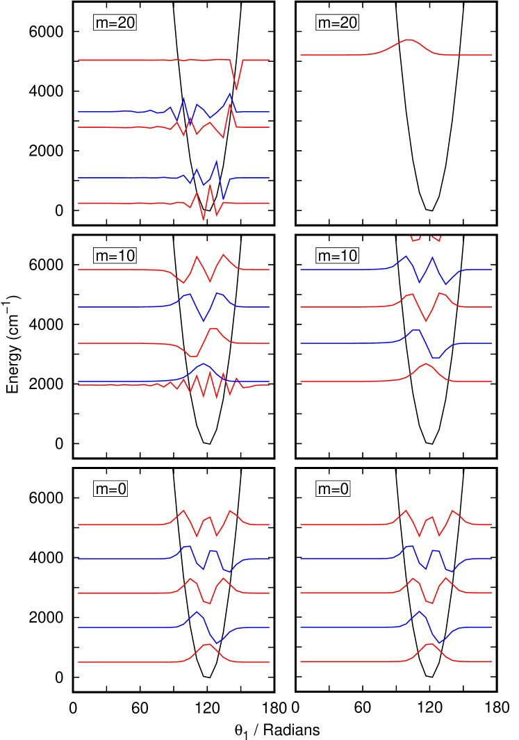
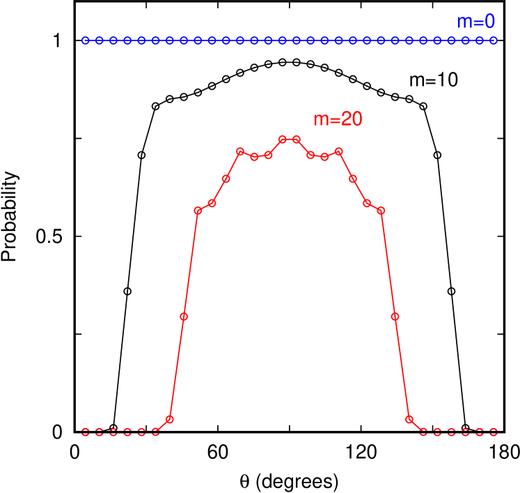
To illustrate the problem and the solution of this problem in Fig. 11 the mono-dimensional eigenfunctions for are shown, which are obtained with and without the projection technique to push up the spurious solutions for different -values, the projection of in the body-fixed frame. For =0, no difference is found. For , the first eigen-function is spurious and it disappears when the projection up technique is applied. For =20 the situation is even worse, and at least five spurious states appears, which are corrected and pushed up. This problem is very notorious when calculating bound states, because the lower eigen values are mainly spurious. In wave packet propagations, this problem is in the angular representation of the Hamiltonian, and it becomes less evident, but this problem is a source of inaccuracies.
References
- Berné et al. (2023) O. Berné, M.-A. Martin-Drumel, I. Schroetter, and et al., Nature 621, 56 (2023).
- Gärtner et al. (2013) S. Gärtner, J. Krieg, A. Klemann, O. Asvany, S. Brünken, and S. Schlemmer, J. Phys. Chem. A 112, 9975 (2013).
- Jusko et al. (2017) P. Jusko, A. Stoffels, S. Thorwirthi, S. Brünken, S. Schlemmer, and O. Asvany, J. Mol. Spectroscopy 332, 59 (2017).
- Töpfer et al. (2018) M. Töpfer, T. Salomon, H. Kohguchi, O. Dopfer, K. M. T. Yamada, S. Schlemmer, and O. Asvany, Phys. Rev. Lett. 121, 143001 (2018).
- Roueff et al. (2013) E. Roueff, M. Guerin, D. C. Lis, A. Wootten, N. Marcelino, J. Cernicharo, and B. Tercero, J. Phys. Chem. A 117, 9959 (2013).
- Gerin et al. (2016) M. Gerin, D. A. Neufeld, and J. R. Goicoechea, Ann. Rev. Astron. Astrophys. 54, 181 (2016).
- Prakash and v. R. Schleyer (1997) G. K. S. Prakash and P. v. R. Schleyer, Stable carbocation chemistry (John Wiley and Sons, New York, 1997).
- Olah and Orakash (2004) G. A. Olah and G. K. S. Orakash, Carbocation chemistry (John Wiley and Sons, Hoboken, 2004).
- Crofton et al. (1988) M. W. Crofton, M.-F. Jagod, B. D. Rehfuss, W. A. Kreiner, and T. Oka, J. Chem. Phys. 88, 666 (1988).
- Jagod et al. (1992) M. Jagod, M. Rösslein, M.-F. Gabrys, D. D. Rehfuss, F. Scappini, M. W. Crofton, and T. Oka, J. Chem. Phys. 97, 7111 (1992).
- White et al. (1999) E. T. White, J. Tang, and T. Oka, Science 284, 135 (1999).
- Wang et al. (2013) H. Wang, C. Neese, C. Morong, M. Kleshcheva, and T. Oka, J. Phys. Chem. A 117, 9908 (2013).
- Gerlich et al. (1987) D. Gerlich, R. Disch, and S. Scherbarth, J. Chem. Phys. 87, 350 (1987).
- Hierl et al. (1997) P. M. Hierl, R. A. Morris, and A. A. Viggiano, J. Chem. Phys. 106, 10145 (1997).
- A. G. G. M. Tielens and D. Hollenbach (1985) A. G. G. M. Tielens and D. Hollenbach, AstroPhys. J. 291, 722 (1985).
- Sternberg and Dalgarno (1995) A. Sternberg and A. Dalgarno, AstroPhys. J. Suppl. 99, 565 (1995).
- Agúndez et al. (2010) M. Agúndez, J. R. Goicoechea, J. Cernicharo, A. Faure, and E. Roueff, AstroPhys. J. , 662 (2010).
- Kaplan et al. (2017) K. F. Kaplan, H. L. Dinerstein, H. Oh, G. N. Mace, H. Kim, K. R. Sokal, M. D. Pavel, S. Lee, S. Pak, C. Park, J. Sok Oh, and D. T. Jaffe, AstroPhys. J. 838, 152 (2017).
- Kaplan et al. (2021) K. F. Kaplan, H. L. Dinerstein, H. Kim, and D. T. Jaffe, AstroPhys. J. 919, 27 (2021).
- Zanchet et al. (2013) A. Zanchet, B. Godard, N. Bulut, O. Roncero, P. Halvick, and J. Cernicharo, ApJ 766, 80 (2013).
- Faure et al. (2017) A. Faure, P. Halvick, T. Stoecklin, P. Honvault, E. Epe, J. Z. Mezei, O. Motapon, I. F. Schneider, J. Tennyson, O. Roncero, N. Bulut, and A. Zanchet, Mon. Not. Royal Astronm. Soc. 469, 612 (2017).
- Smith et al. (1982) D. Smith, N. G. Adams, and E. Alge, J. Chem. Phys. 77, 1261 (1982).
- Asvanay et al. (2004) O. Asvanay, S. Schlemmer, and D. Gerlich, AstroPhys. J. 617, 685 (2004).
- Asvany et al. (2018) O. Asvany, S. Thorwirth, B. Redlich, and S. Schlemmer, J. Mol. Spectroscopy , 1 (2018).
- R. Signorell and F. Merkt (1999) R. Signorell and F. Merkt, J. Chem. Phys. 110, 2309 (1999).
- Wörner et al. (2006) H. J. Wörner, R. van der Veen, and F. Merkt, Phys. Rev. Lett. 97, 173003 (2006).
- Asvany et al. (2004) P. Asvany, I. Savic, S. Schlemmer, and D. Gerlich, Chem. Phys. 298, 97 (2004).
- Schreiner et al. (1993) P. R. Schreiner, S.-J. Kim, H. F. S. III, and P. von Rague Schleyer, J. Chem. Phys. 99, 3716 (1993).
- Asvany et al. (2015) O. Asvany, K. M. T. Yamada, S. Brünken, A. Potapov, and S. Schlemmer, Science 347, 1346 (2015).
- Dalgarno (1985) A. Dalgarno, in Proceedings of the Advanced Research Workshop, Bad Windsheim, West Germany, July 8-14, 1984 (A86-39726 18-90), edited by G. H. F. Dierksen, W. F. Huebner, and P. W. Langhoff (Dordretch: Springer Netherlands, 1985) p. 3.
- Wakelam et al. (2010) V. Wakelam, I. Smith, E. Herbst, J. Troe, W. Geppert, H. Linnartz, K. Öberg, E. Roueff, M. Agúndez, P. Pernot, H. M. Cuppen, J. C. Loison, and D. Talbi, Space Science Rev. 156, 13 (2010).
- Chabot et al. (2020) M. Chabot, T. IdBarkach, K. Béroff, F. L. Petit, and V. Wakelam, Astron. AstroPhys. 640, 115 (2020).
- Henning et al. (2024) T. Henning, I. Kamp, M. Samland, A. M. Arabhavi, J. Kanwar, E. F. van Dishoeck, M. Guedel, P.-O. Lagage, C. Waelkens, A. Abergel, O. Absil, D. Barrado, A. Boccaletti, J. Bouwman, A. C. o. Garatti, V. Geers, A. M. Glauser, F. Lahuis, C. Nehme, G. Olofsson, E. Pantin, T. P. Ray, B. Vandenbussche, L. B. F. M. Waters, G. Wright, V. Christiaens, R. Franceschi, D. Gasman, R. Guadarrama, H. Jang, M. Morales-Calderon, N. Pawellek, G. Perotti, D. Rodgers-Lee, J. Schreiber, K. Schwarz, B. Tabone, M. Temmink, M. Vlasblom, L. Colina, T. R. Greve, and G. Oestlin, arXiv e-prints , arXiv:2403.09210 (2024), arXiv:2403.09210 [astro-ph.EP] .
- Kraemer and Spirko (1991) W. P. Kraemer and V. Spirko, J. Mol. Spectroscopy 149, 235 (1991).
- Yu and Sears (2002) H.-G. Yu and T. J. Sears, J. Chem. Phys. 117, 666 (2002).
- Nyman and Yu (2019) G. Nyman and H.-G. Yu, AIP advances 9, 095017 (2019).
- Changala, P. B. et al. (2023) Changala, P. B., Chen, N. L., Le, H. L., Gans, B., Steenbakkers, K., Salomon, T., Bonah, L., Schroetter, I., Canin, A., Martin-Drumel, M.-A., Jacovella, U., Dartois, E., Boyé-Péronne, S., Alcaraz, C., Asvany, O., Brünken, S., Thorwirth, S., Schlemmer, S., Goicoechea, J. R., Rouillé, G., Sidhu, A., Chown, R., Van De Putte, D., Trahin, B., Alarcón, F., Berné, O., Habart, E., and Peeters, E., Astron. AstroPhys. 680, A19 (2023).
- Crofton et al. (1985) M. W. Crofton, W. A. Kreiner, M.-F. Jagod, B. D. Rehfuss, and T. Oka, J. Chem. Phys. 83, 3702 (1985).
- Blush et al. (1993) J. A. Blush, P. Chen, R. T. Wiedmann, and M. G. White, J. Chem. Phys. 98, 3557 (1993).
- Wiedmann et al. (1994) R. T. Wiedmann, M. G. White, K. Wang, and V. McKoy, J. Chem. Phys. 100, 4738 (1994).
- Liu et al. (2001) X. Liu, R. L. Gross, and A. G. Suits, Science 294, 2527 (2001).
- Schulenburg et al. (2006) A. M. Schulenburg, C. Alcaraz, G. Grassi, and F. Merkt, J. Chem. Phys. 125, 104310 (2006).
- Taatjes et al. (2008) C. A. Taatjes, D. L. Osborn, T. M. Selby, G. Meloni, H. Fan, and S. T. Pratt, J. Phys. Chem. A 112, 9336 (2008).
- Loison (2010) J.-C. Loison, J. Phys. Chem. A 114, 6515 (2010).
- B. K. Cunha de Miranda and C. Alcaraz and M. Elhanine and B. Noller and P. Hemberger and I. Fischer and G. A. Garcia and H. Soldi-Lose⊥ and B. Gans and L. A. Vieira Mendes and S. Boyé-Péronne and S. Douin and J. Zabka and P. Botschwina (2010) B. K. Cunha de Miranda and C. Alcaraz and M. Elhanine and B. Noller and P. Hemberger and I. Fischer and G. A. Garcia and H. Soldi-Lose and B. Gans and L. A. Vieira Mendes and S. Boyé-Péronne and S. Douin and J. Zabka and P. Botschwina, J. Phys. Chem. A 114, 4818 (2010).
- B. Gans and L. A. Vieira Mendes and S. Boyé-Pérone and S. Douin and G. García and H. Soldi-Lose and B. Cunha de Miranda anid C. Alcaraz and N. Carrasco and P. Pernot and D. Gauyacq (2010) B. Gans and L. A. Vieira Mendes and S. Boyé-Pérone and S. Douin and G. García and H. Soldi-Lose and B. Cunha de Miranda anid C. Alcaraz and N. Carrasco and P. Pernot and D. Gauyacq, J. Phys. Chem. A 114, 3237 (2010).
- Heays et al. (2017) A. N. Heays, A. D. Bosman, and E. F. van Dishoeck, Astron. AstroPhys. 602, A105 (2017).
- Blint et al. (1976) R. J. Blint, R. F. Marshall, and W. D. Watson, AstroPhys. J. 206, 627 (1976).
- Tielens (2010) A. Tielens, The Physics and Chemistry of the Interstellar Medium (Cambridge University Press, 2010).
- Werner and Knowles (1988) H. J. Werner and P. J. Knowles, J. Chem. Phys. 89, 5803 (1988).
- Shiozaki and Werner (2011) T. Shiozaki and H.-J. Werner, J. Chem. Phys. 134, 184104 (2011).
- Werner et al. (2012) H.-J. Werner, P. J. Knowles, G. Knizia, F. R. Manby, and M. Schütz, WIREs Comput Mol Sci 2, 242 (2012).
- Hill et al. (2010) J. Hill, S. Maxumder, and K. Peterson, J.Chem. Phys. 132, 054108 (2010).
- Delsaut (2015) M. Delsaut, Methyl Cation in Astrochemistry: ab initio study of its formation, Ph.D. thesis, Faculté des Sciences, Université Libre de Bruxelles, (2015).
- Shao et al. (2016) K. Shao, J. Chen, Z. Zhao, and D. H. Zhang, Journal of Chemical Physics 145, 071101 (2016).
- (56) “Github repository with fi definitions,” https://github.com/pablomazo/FI, accessed: 2024-01-09.
- del Mazo-Sevillano et al. (2021) P. del Mazo-Sevillano, A. Aguado, and O. Roncero, The Journal of Chemical Physics 154, 094305 (2021).
- del Mazo-Sevillano et al. (2023) P. del Mazo-Sevillano, D. Félix-González, A. Aguado, C. Sanz-Sanz, D. Kwon, and O. Roncero, Mol. Phys. , e2183071 (2023).
- Paszke et al. (2019) A. Paszke, S. Gross, F. Massa, A. Lerer, J. Bradbury, G. Chanan, T. Killeen, Z. Lin, N. Gimelshein, L. Antiga, A. Desmaison, A. Kopf, E. Yang, Z. DeVito, M. Raison, A. Tejani, S. Chilamkurthy, B. Steiner, L. Fang, J. Bai, and S. Chintala, in Advances in Neural Information Processing Systems 32, edited by H. Wallach, H. Larochelle, A. Beygelzimer, F. d’Alché Buc, E. Fox, and R. Garnett (Curran Associates, Inc., 2019) pp. 8024–8035.
- Liu and Nocedal (1989) D. C. Liu and J. Nocedal, Mathematical Programming 45, 503 (1989).
- Yu and Muckerman (2002) H.-G. Yu and J. T. Muckerman, J. Mol. Spectroscopy , 11 (2002).
- Cullum and Willoughby (1985) J. Cullum and R. Willoughby, Lanczos Algorithms for Large Symmetric Eigenvalues Computations (Birkhäuser, Boston, 1985).
- Fröberg (1985) C.-E. Fröberg, Numerical Mathematics: Theory and Computer Applications (The Benjamin/Cummings Publishing Company, 1985).
- Wyatt (1989) R. E. Wyatt, Adv. Chem. Phys. LXXIII, 231 (1989).
- Smith (1980) F. T. Smith, Phys. Rev. Lett. 45, 1157 (1980).
- Zare (1988) R. Zare, Angular Momentum (John Wiley and Sons, Inc., 1988).
- Colbert and Miller (1992) D. T. Colbert and W. H. Miller, J. Chem. Phys. 96, 1982 (1992).
- Corey and Lemoine (1992) G. C. Corey and D. Lemoine, J. Chem. Phys. 97, 4115 (1992).
- Corey et al. (1993) G. C. Corey, J. W. Tromp, and D. Lemoine, in Numerical grid methods and their application to Schrödinger equation, edited by C. Cerjan (Kluwer Academic Publishers, 1993) p. 1.
- Goldfield (2000) E. M. Goldfield, Comp. Phys. Comm. 128, 178 (2000).
- Lin and Guo (2002) S. Y. Lin and H. Guo, J. Chem. Phys. 117, 5183 (2002).
- Mowrey (1991) R. C. Mowrey, J. Chem. Phys. 94, 7098 (1991).
- Guan et al. (2020) Y. Guan, H. Guo, and D. R. Yarkony, Journal of Chemical Theory and Computation 16, 302 (2020), https://doi.org/10.1021/acs.jctc.9b00898 .
- Herzberg and Longuet-Higgins (1963) G. Herzberg and H. C. Longuet-Higgins, Discuss. Faraday 35, 77 (1963).
- Berry (1984) M. V. Berry, Proc. R. Soc. Lond. A392, 4557 (1984).
- Xie et al. (2017) C. Xie, D. R. Yarkony, and H. Guo, Phys. Rev. A 95, 022104 (2017).
- Mandelshtam and Taylor (1995) V. A. Mandelshtam and H. S. Taylor, J. Chem. Phys. 102, 7390 (1995).
- Chen and Guo (1996) R. Chen and H. Guo, J. Chem. Phys. 105, 3569 (1996).
- Gray and Balint-Kurti (1998) S. K. Gray and G. G. Balint-Kurti, J. Chem. Phys. 108, 950 (1998).
- González-Lezana et al. (2005) T. González-Lezana, A. Aguado, M. Paniagua, and O. Roncero, J. Chem. Phys. 123, 194309 (2005).
- Paniagua et al. (1999) M. Paniagua, A. Aguado, M. Lara, and O. Roncero, J. Chem. Phys. 111, 6712 (1999).
- Aguado et al. (2003) A. Aguado, M. Paniagua, C. Sanz-Sanz, and O. Roncero, J. Chem. Phys. 119, 10088 (2003).
- Chenel et al. (2016) A. Chenel, O. Roncero, A. Aguado, M. Agúndez, and J. Cernicharo, J. Chem. Phys. 144, 144306 (2016).
- Draine (1978) Draine, AstroPhysical J. 37, 595 (1978).
- Le Petit et al. (2006) F. Le Petit, C. Nehmé, J. Le Bourlot, and E. Roueff, Astrophys. J. 164, 506 (2006), astro-ph/0602150 .
- Goicoechea and Le Bourlot (2007) J. R. Goicoechea and J. Le Bourlot, Astronomy Astrophys. 467, 1 (2007), astro-ph/0702033 .
- Goicoechea et al. (2016) J. R. Goicoechea, J. Pety, S. Cuadrado, J. Cernicharo, E. Chapillon, A. Fuente, M. Gerin, C. Joblin, N. Marcelino, and P. Pilleri, Nature 537, 207 (2016), arXiv:1608.06173 .