*mainfig/extern/\finalcopy
A Learning Paradigm for Interpretable Gradients
Abstract
This paper studies interpretability of convolutional networks by means of saliency maps. Most approaches based on Class Activation Maps (CAM) combine information from fully connected layers and gradient through variants of backpropagation. However, it is well understood that gradients are noisy and alternatives like guided backpropagation have been proposed to obtain better visualization at inference. In this work, we present a novel training approach to improve the quality of gradients for interpretability. In particular, we introduce a regularization loss such that the gradient with respect to the input image obtained by standard backpropagation is similar to the gradient obtained by guided backpropagation. We find that the resulting gradient is qualitatively less noisy and improves quantitatively the interpretability properties of different networks, using several interpretability methods.
1 INTRODUCTION
The improvement of deep learning models in the last decade has led to their adoption and penetration into most application sectors. Since these models are highly complex and opaque, the requirement for interpretability of their predictions receives a lot of attention [Lipton, 2018]. Explanation and transparency becomes a legal requirements for systems used in high-stakes and high-risk decisions.
In this work, we focus on the visual interpretability of deep learning models. Model interpretability is often categorized into transparency and post-hoc methods. Transparency aims at producing models where the inner process or part of it can be understood. Post-hoc methods consider models as black-boxes and interpret decisions mainly based on inputs and outputs.
In visual recognition, most methods focus on post-hoc interpretability by means of saliency maps. These maps highlight the most important areas of an image related to the network prediction. Initial works focused on using gradients for visualization, such as guided backpropagation [Springenberg et al., 2014]. CAM [Zhou et al., 2016] later proposed a class-specific linear combination of feature maps and opened the way to numerous weighting strategies.
Most CAM-based methods use backpropagation in one way or another. Recognizing that the gradients obtained this way are noisy, methods like SmoothGrad [Smilkov et al., 2017] and SmoothGrad-CAM++ [Omeiza et al., 2019] improve the quality of saliency maps by denoising the gradients. However, this requires several forward passes, thus comes with increased cost at inference.
In this work, we rather propose a learning paradigm for model training that regularizes gradients to improve the performance of interpretability methods. In particular, we add a regularization term to the loss function that encourages the gradient in the input space to align with the gradient obtained by guided back-propagation. This has a smoothing effect on gradient and is shown to improve the power of model interpretations.
Figure 1 summarizes our method. At training, each input image is forwarded through the network to compute the cross-entropy loss. Standard and guided backpropagation is performed back to the input image space, where our regularization term is computed. This term is added to the loss and backpropagated only through the standard backpropagation branch.
The key contributions of this work are as follows:
-
•
We introduce a new learning paradigm to regularize gradients.
-
•
Using different networks, we show that our method improves the gradient quality and the performance of several interpretability methods using multiple metrics, while preserving accuracy.
2 RELATED WORK
Interpretability of deep neural network decisions is a problem that receives increasing interest. As interpretability is not simple to define, Lipton [Lipton, 2018] proposes some common ground, definitions and categorization for interpretability methods. For instance, transparency aims at making models simple so it is humanly possible to provide an explanation of its inner mechanism. By contrast, post-hoc methods consider models as black boxes and study the activations leading to a specific output.
LIME [Ribeiro et al., 2016] and SHAP [Lundberg and Lee, 2017] are probably the most popular post-hoc methods that are model agnostic and provide local information. Concerning image recognition tasks, it is common to generate saliency maps highlighting the areas of an image that are responsible for a specific prediction. Several of these methods are either based on backpropagation and its variants or on Class Activation Maps (CAM) that weigh the importance of activation maps.
2.1 Gradient-based approaches
Gradient-based approaches assess the impact of distinct image regions on the prediction based on the partial derivative of the model prediction function with respect to the input. A simple saliency map can be the partial derivative obtained by a single backward pass through the model [Simonyan et al., 2014].
Guided backpropagation [Springenberg et al., 2014] enhances explanations by removing negative gradients through ReLU units. For better visualization, SmoothGrad [Smilkov et al., 2017] applies noise to the input and derives saliency maps based on the average of resulting gradients. Layer-wise Relevance Propagation (LRP) [Bach et al., 2015] reallocates the prediction score through a custom backward pass across the network.
Our method has a similar objective as SmoothGrad [Smilkov et al., 2017] but instead of using several forward passes at inference, we regularize gradients using guided backpropagation during training. Thus we obtain better gradients without modifying the inference process and our method can be used with any interpretability method at inference.
2.2 CAM-based approaches
Class Activation Maps [Zhou et al., 2016] produces a saliency map that highlights the areas of an image that are the most responsible for a CNN decision. The saliency map is computed as a linear combinations of feature maps from a given layer. Different variants of CAM are proposed by defining different weighting coefficients. Grad-CAM [Selvaraju et al., 2017], for instance, spatially averages the gradient with respect to feature maps. Grad-CAM++ [Chattopadhay et al., 2018] improves object localization by using positive partial derivatives and measuring recognition and localization metrics.
It is possible to extend CAM to multiple layers [Jiang et al., 2021] and to improve sensitivity [Sundararajan et al., 2017] and conservation [Montavon et al., 2018] by the addition of axioms [Fu et al., 2020]. Score-CAM [Wang et al., 2020] is a gradient-free method that computes weighting coefficients by maximizing the Average Increase metric [Chattopadhay et al., 2018]. Further improvement can be obtained by means of test-time optimization [Zhang et al., 2023].
Some works provide explanations that not only localize salient parts of images, but also provide theoretical bases on the effect of modifying such regions for a given input [Fu et al., 2020]. An exhaustive alternative performs ablation experiments to highlight such parts [Ramaswamy et al., 2020].
All these approaches apply at inference, without modifying the model or the training process. By contrast, our work applies at training with the objective of improving the quality of gradients, which is much needed for gradient-based methods. Thus, our method is orthogonal and can be used with any of these approaches at inference.
2.3 Double backpropagation
Double backpropagation is a general regularization paradigm, first introduced by Drucker and Le Cun [Drucker and Le Cun, 1991] to improve generalization. The idea is used to avoid overfitting [Philipp and Carbonell, 2018], help transfer [Srinivas and Fleuret, 2018], cope with noisy labels [Luo et al., 2019], and more recently to increase adversarial robustness [Lyu et al., 2015, Simon-Gabriel et al., 2018, Ross and Doshi-Velez, 2018, Seck et al., 2019, Finlay et al., 2018]. It aims at penalizing the [Seck et al., 2019], or norm of the gradient with respect to the input image.
Our method is related and regularizes the standard gradient by aligning it with the guided gradient, obtained by guided backpropagation [Springenberg et al., 2014].
3 BACKGROUND
3.1 Guided backpropagation
The derivative of with respect to is . By the chain rule, a signal is then propagated backwards through the unit to as , where is the partial derivative of any scalar quantity of interest, e.g. a loss , with respect to .
Guided backpropagation [Springenberg et al., 2014] changes this to , masking out values corresponding to negative entries of both the forward () and the backward () signals and thus preventing backward flow of negative gradients.
Standard backpropagation through an entire network with this particular change for units is called guided backpropagation. The corresponding guided “partial derivative” or guided gradient of scalar quantity with respect to is denoted by . This method allows sharp visualization of high-level activations conditioned on input images.
3.2 CAM-based methods
CAM-based methods build a saliency map as a linear combination of feature maps. Given a target class and a set of 2D feature maps , the saliency map is defined as
| (1) |
where the weight determines the contribution of channel to class . The saliency map and the feature maps are both non-negative because of using activation functions. Different CAM-based methods differ primarily in the definition of the weights .
CAM [Zhou et al., 2016]
originally defines as the weight connecting channel to class in the classifier, assuming are the feature maps of the last convolutional layer, which is followed by global average pooling (GAP) and a fully connected layer.
Grad-CAM [Selvaraju et al., 2017]
is a generalization of CAM for any network. If is the logit of class , the weights are obtained by GAP of the partial derivatives of with respect to elements of feature map of any given layer,
| (2) |
where denotes the value at spatial location of feature map and is the total number of locations.
Guided Grad-CAM elementwise-multiplies the saliency maps obtained by Grad-CAM and guided backpropagation, after adjusting spatial resolutions. The resulting visualizations are both class-discriminative (by Grad-CAM) and contain fine-grained detail (by guided backpropagation).
Grad-CAM++ [Chattopadhay et al., 2018]
is a generalization of Grad-CAM, where partial derivatives of with respect to are followed by as in guided backpropagation and GAP is replaced by a weighted average:
| (3) |
The weights of the linear combination are
| (4) |
Score-CAM [Wang et al., 2020]
computes the weights based on the increase in confidence [Chattopadhay et al., 2018] for class obtained by masking (element-wise multiplying) the input image with feature map :
| (5) |
where is upsampling to the spatial resolution of , is linear normalization to range , is the Hadamard product, is the network mapping of input image to class probability vectors and is a baseline image.
While Score-CAM does not require gradients to compute saliency maps, (5) requires one forward pass through the network for each channel .
4 METHOD
Preliminaries
We consider an image classification network with parameters , which maps an input image to a vector of predicted class probabilities . At inference, we predict the class of maximum confidence , where is the probability of class . At training, given training images and target labels , we compute the classification loss
| (6) |
where is cross-entropy:
| (7) |
Updates of parameters are performed by an optimizer, based on the standard partial derivative (gradient) of the classification loss with respect to , obtained by standard back-propagation.
Motivation
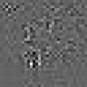
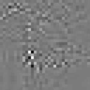
Due to non-linearities like ReLU activations and downsampling like max-pooling or convolution stride greater than , the standard gradient is noisy [Smilkov et al., 2017]. This is shown by visualizing the gradient with respect to an input image . By contrast, the guided gradient [Springenberg et al., 2014] does not suffer much from noise and preserves sharp details. The difference of the two gradients is illustrated in Figure 1.
The main motivation of this work is that introducing a regularization term during training could make the standard gradient behave similarly to the corresponding guided gradient , while maintaining the predictive power of the classifier . We hypothesize that, if this is possible, it will improve the quality of all gradients with respect to intermediate activations and therefore the quality of saliency maps obtained by CAM-based methods [Zhou et al., 2016, Selvaraju et al., 2017, Chattopadhay et al., 2018, Wang et al., 2020] and the interpretability of network . The effect may be similar to that of SmoothGrad [Smilkov et al., 2017], but without the need for several forward passes at inference.
Regularization
Given an input training image and its target labels , we perform a forward pass through and compute the probability vectors and the contribution of to the classification loss (6).
We then obtain the standard gradients and the guided gradients with respect to by two separate backward passes. Since the whole process is differentiable (w.r.t. ) at training, we stop the gradient computation of the latter, so that it only serves as a “teacher”. We define the regularization loss
| (8) |
where is an error function between the two gradient images, considered below.
The total loss is defined as
| (9) |
where is a hyperparameter determining the regularization strength. should be large enough to smooth the gradient without decreasing the classification accuracy or harming the training process.
Updates of the network parameters are based on the standard gradient of the total loss w.r.t. , using any optimizer. At inference, one may use any interpretability method to obtain a saliency map at any layer.
Error function
Given two gradient images consisting of pixels each, we consider the following error functions to compute the regularization loss (8).
-
1.
Mean absolute error (MAE):
(10) -
2.
Mean squared error (MSE):
(11)
We also consider the following two similarity functions, with a negative sign.
-
3.
Cosine similarity:
(12) where denotes inner product.
-
4.
Histogram intersection (HI):
(13)
Algorithm
Our method is summarized in algorithm 1 and illustrated in Figure 1. It is interesting to note that the entire computational graph depicted in Figure 1 involves one forward and two backward passes. This graph is then differentiated again to compute , which involves one more forward and backward pass, since the guided backpropagation branch is excluded. Thus, each training iteration requires five passes through instead of two in standard training.
5 EXPERIMENTS
5.1 Experimental setup
In the following sections, we evaluate the effect of our approach on recognition and interpretability.
Models and datasets
We train and evaluate a ResNet-18 [He et al., 2016] and a MobileNet-V2 [Sandler et al., 2018] on CIFAR-100 [Krizhevsky, 2009]. ResNets are the most common CNNs and the ResNet-18 is particularly adapted to low resolution images. MobileNet-V2 is a widely used compact CNN. CIFAR-100 contains 60.000 images of 100 categories, split in 50.000 for training and 10.000 for testing. Each image has a resolution of pixels.
Settings
To obtain competitive performance and ensure the replicability of our method, we follow the methodology by weiaicunzai111https://github.com/weiaicunzai/pytorch-cifar100. In particular, we train for 200 epochs, with a batch-size of 128 images, SGD optimizer, initial learning rate and learning rate decay by a factor of 5 on epochs 60, 120 and 160.
At inference, we generate explanations following popular attribution methods derived from CAM [Zhou et al., 2016], from the pytorch-grad-cam library from Jacob Gildenblat222https://github.com/jacobgil/pytorch-grad-cam.
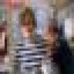
| Input | Grad-CAM | Grad-CAM++ | Score-CAM | Ablation-CAM | |||||
|---|---|---|---|---|---|---|---|---|---|
| Baseline | Ours | Baseline | Ours | Baseline | Ours | Baseline | Ours | ||
|
Man |
 |
 |
 |
 |
 |
 |
 |
 |
 |
|
Girl |
 |
 |
 |
 |
 |
 |
 |
 |
 |
|
Woman |
 |
 |
 |
 |
 |
 |
 |
 |
 |
|
Lobster |
 |
 |
 |
 |
 |
 |
 |
 |
 |
|
Couch |
 |
 |
 |
 |
 |
 |
 |
 |
 |
5.2 Faithfulness metrics
Faithfulness evaluation [Chattopadhay et al., 2018] offers insight on the regions of an image that are considered important for recognition, as highlighted by the saliency map . Specifically, given a target class , an image and a saliency map are element-wise multiplied to obtain a masked image
This masked image is similar to the original image on the salient areas and black on the non-salient ones. To evaluate the quality of saliency maps, we forward both the original image and its masked version through the network to obtain the predicted probabilities and respectively. We then compute a number of metrics as defined below.
Average Drop (AD)
aims at quantifying how much predictive power is lost when we consider the masked image compared to the original one. Lower is better.
| (14) |
Average Increase (AI)
is also known as Increase of Confidence and measures the percentage of examples of the dataset where the masked image offers a higher probability than the original for the target class. Higher is better.
| (15) |
Average Gain (AG)
is recently introduced in [Zhang et al., 2023] and designed to be a symmetric complement of AD, replacing AI. It aims at quantifying how much predictive power is gained when we consider the masked image compared to the original one. Higher is better.
| (16) |
5.3 Causal metrics
Causality evaluation [Petsiuk et al., 2018] aims at evaluating the effect of masking certain elements of the image in the predictive power of a model. Two metrics are defined as follows. Histograms and average values can be computed per image. Following most previous work, we only show average values over the test set.
Insertion
starts from a blurry image and gradually inserts (unblurs) pixels of the original image, ranked by decreasing saliency as defined in a given saliency map. At each iteration, images are passed through the network to compute the predicted probabilities and compare to the original.
Deletion
gradually removes the pixels by replacing them by black, starting from the most salient pixels. As for insertion, we compute the predicted probabilities at each iteration.
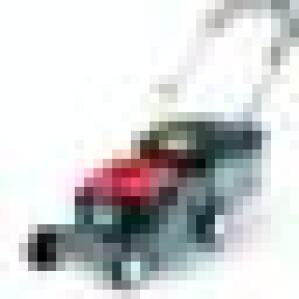
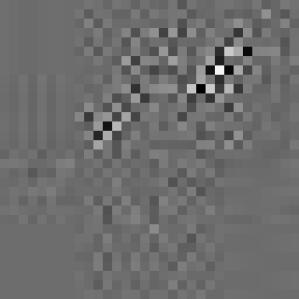
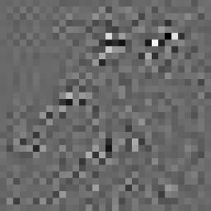
| Input | Baseline | Ours | |
|---|---|---|---|
|
Bed |
 |
 |
 |
|
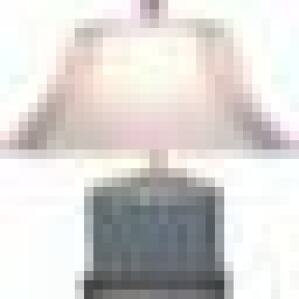
Lamp |
 |
 |
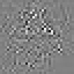 |
|
Lawnmower |
 |
 |
 |
|
Maple Tree |
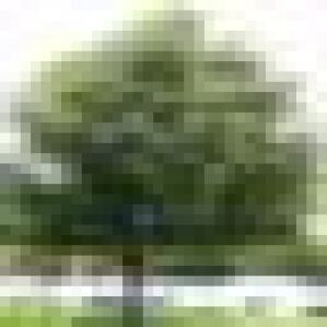 |
 |
 |
|
Sunflower |
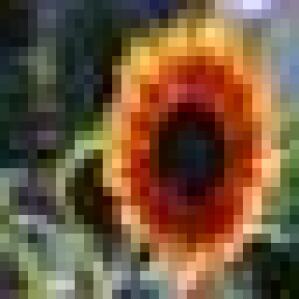 |
 |
 |
5.4 Qualitative results
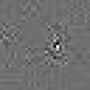
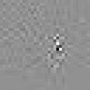
We visualize the effect of our approach on saliency maps and gradients, obtained for the baseline model vs. the one trained with our approach.
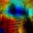
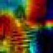
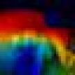
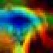
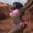
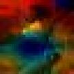
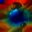
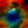
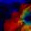
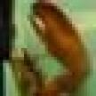
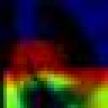
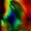
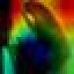
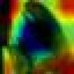
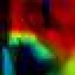
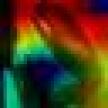
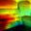
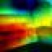
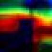
Figure 2 shows saliency maps. We observe the differences brought by our training method. The differences are particularly important for Grad-CAM, which directly averages the gradient to weigh feature maps. Interestingly, the differences are smaller for Score-CAM, which is not gradient-based but only obtains changes of predicted probabilities.
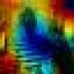
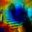
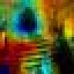
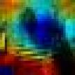
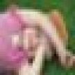
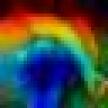
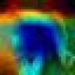
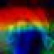
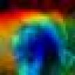
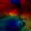
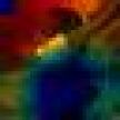
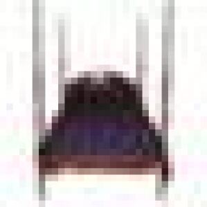
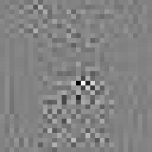
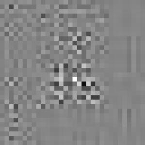
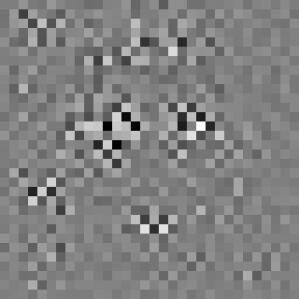
Figure 3 shows gradients. We observe slightly less noise with our method, while the object of interest is better covered by gradient activations.
| Model | Error | Acc | |
|---|---|---|---|
| ResNet-18 | Baseline | – | 73.42 |
| Ours | 72.86 | ||
| MobileNet-V2 | Baseline | – | 59.43 |
| Ours | 62.36 |
| ResNet-18 | ||||||
|---|---|---|---|---|---|---|
| Method | Error | AD | AG | AI | Ins | Del |
| Grad-CAM | Baseline | 30.16 | 15.23 | 29.99 | 58.47 | 17.47 |
| Ours | 28.09 | 16.19 | 31.53 | 58.76 | 17.57 | |
| Grad-CAM++ | Baseline | 31.40 | 14.17 | 28.47 | 58.61 | 17.05 |
| Ours | 29.78 | 15.07 | 29.60 | 58.90 | 17.22 | |
| Score-CAM | Baseline | 26.49 | 18.62 | 33.84 | 58.42 | 18.31 |
| Ours | 24.82 | 19.49 | 35.51 | 59.11 | 18.34 | |
| Ablation-CAM | Baseline | 31.96 | 14.02 | 28.33 | 58.36 | 17.14 |
| Ours | 29.90 | 15.03 | 29.61 | 58.70 | 17.37 | |
| Axiom-CAM | Baseline | 30.16 | 15.23 | 29.98 | 58.47 | 17.47 |
| Ours | 28.09 | 16.20 | 31.53 | 58.76 | 17.57 | |
| MobileNet-V2 | ||||||
| Method | Error | AD | AG | AI | Ins | Del |
| Grad-CAM | Baseline | 44.64 | 6.57 | 25.62 | 44.64 | 14.34 |
| Ours | 40.89 | 7.31 | 27.08 | 45.57 | 15.20 | |
| Grad-CAM++ | Baseline | 45.98 | 6.12 | 24.10 | 44.72 | 14.76 |
| Ours | 40.76 | 6.85 | 26.46 | 45.51 | 14.92 | |
| Score-CAM | Baseline | 40.55 | 7.85 | 28.57 | 45.62 | 14.52 |
| Ours | 36.34 | 9.09 | 30.50 | 46.35 | 14.72 | |
| Ablation-CAM | Baseline | 45.15 | 6.38 | 25.32 | 44.62 | 15.03 |
| Ours | 41.13 | 7.03 | 26.10 | 45.38 | 15.12 | |
| Axiom-CAM | Baseline | 44.65 | 6.57 | 25.62 | 44.64 | 15.27 |
| Ours | 40.89 | 7.31 | 27.08 | 45.57 | 15.20 | |
5.5 Quantitative results
We evaluate the effect of training a given model using our proposed approach with faithfulness and causality metrics. As shown in Table 1 and Table 2, we obtain improvements on both networks and on four out of five interpretability metrics, while remaining within half percent or improving accuracy relative to the baseline, standard backpropagation.
The improvements are higher for faithfulness metrics AD, AG, and AI. Insertion gets a smaller but consistent improvement. Deletion is mostly inferior with our method, but with a very small difference. This may be due to limitations of the metrics, as reported in previous works [Zhang et al., 2023].
It is interesting to note that improvements on Score-CAM mean that our training not only improves gradient but also builds better activation maps, since Score-CAM only relies on those.
| Error function | Acc | AD | AG | AI | Ins | Del |
|---|---|---|---|---|---|---|
| Baseline | 73.42 | 30.16 | 15.23 | 29.99 | 58.47 | 17.47 |
| Cosine | 72.86 | 28.09 | 16.19 | 31.53 | 58.76 | 17.57 |
| Histogram | 73.88 | 30.39 | 14.78 | 29.38 | 58.52 | 17.35 |
| MAE | 73.41 | 30.33 | 15.06 | 29.61 | 58.13 | 17.95 |
| MSE | 73.86 | 29.64 | 15.19 | 30.11 | 59.05 | 18.02 |
| Acc | AD | AG | AI | Ins | Del | |
|---|---|---|---|---|---|---|
| 73.42 | 30.16 | 15.23 | 29.99 | 58.47 | 17.47 | |
| 73.71 | 29.52 | 15.17 | 30.03 | 59.23 | 17.45 | |
| 72.99 | 30.53 | 15.82 | 30.56 | 59.04 | 17.96 | |
| 72.46 | 30.10 | 16.06 | 30.67 | 57.47 | 17.80 | |
| 72.86 | 28.09 | 16.20 | 31.53 | 58.76 | 17.57 | |
| 73.28 | 28.97 | 15.75 | 31.16 | 58.99 | 17.50 | |
| 73.00 | 28.93 | 16.13 | 31.55 | 59.66 | 17.95 | |
| 73.30 | 28.44 | 16.02 | 31.31 | 58.64 | 17.48 | |
| 73.04 | 29.28 | 15.23 | 30.47 | 58.74 | 17.47 |
5.6 Ablation Experiments
Using ResNet-18 and Grad-CAM attributions, we analyze the effect of the error function and the regularization coefficient (9) on our approach.
Error function
As shown in Table 3, we obtain a consistent improvement on most metrics for all error functions. Accuracy remains stable within half percent of the original model. However, most options have little or negative effect on deletion. Cosine similarity provides improvements in most metrics, while maintaining deletion performance. We thus choose cosine error function by default.
Regularization coefficient
As shown in Table 4, our method is not very sensible to the regularization coefficient . The value of works better in general and is thus selected as default.
6 CONCLUSION
In this paper, we propose a new training approach to improve the gradient of a CNN in terms of interpretability. Our method forces the gradient with respect to the input image obtained by backpropagation to align with the gradient coming from guided backpropagation. The results of our training are evaluated according to several interpretability methods and metrics. Our method offers consistent improvement on most metrics for two networks, while remaining within a small margin of the standard gradient in terms accuracy.
7 ACKNOWLEDGEMENT
This work has received funding from the UnLIR ANR project (ANR-19-CE23-0009), the Excellence Initiative of Aix-Marseille Universite - A*Midex, a French “Investissements d’Avenir programme” (AMX-21-IET-017). Part of this work was performed using HPC resources from GENCI-IDRIS (Grant 2020-AD011011853 and 2020-AD011013110).
REFERENCES
- Bach et al., 2015 Bach, S., Binder, A., Montavon, G., Klauschen, F., Müller, K.-R., and Samek, W. (2015). On pixel-wise explanations for non-linear classifier decisions by layer-wise relevance propagation. PloS one, 10(7).
- Chattopadhay et al., 2018 Chattopadhay, A., Sarkar, A., Howlader, P., and Balasubramanian, V. N. (2018). Grad-CAM++: Generalized gradient-based visual explanations for deep convolutional networks. In WACV.
- Drucker and Le Cun, 1991 Drucker, H. and Le Cun, Y. (1991). Double backpropagation increasing generalization performance. In IJCNN.
- Finlay et al., 2018 Finlay, C., Oberman, A. M., and Abbasi, B. (2018). Improved robustness to adversarial examples using Lipschitz regularization of the loss.
- Fu et al., 2020 Fu, R., Hu, Q., Dong, X., Guo, Y., Gao, Y., and Li, B. (2020). Axiom-based Grad-CAM: Towards accurate visualization and explanation of CNNs. arXiv preprint arXiv:2008.02312.
- He et al., 2016 He, K., Zhang, X., Ren, S., and Sun, J. (2016). Deep residual learning for image recognition. In CVPR.
- Jiang et al., 2021 Jiang, P.-T., Zhang, C.-B., Hou, Q., Cheng, M.-M., and Wei, Y. (2021). LayerCAM: Exploring hierarchical class activation maps for localization. TIP.
- Krizhevsky, 2009 Krizhevsky, A. (2009). Learning multiple layers of features from tiny images. pages 32–33.
- Lipton, 2018 Lipton, Z. C. (2018). The mythos of model interpretability: In machine learning, the concept of interpretability is both important and slippery. Queue, 16(3):31–57.
- Lundberg and Lee, 2017 Lundberg, S. M. and Lee, S.-I. (2017). A unified approach to interpreting model predictions. In NeurIPS.
- Luo et al., 2019 Luo, Y., Zhu, J., and Pfister, T. (2019). A simple yet effective baseline for robust deep learning with noisy labels. arXiv preprint arXiv:1909.09338.
- Lyu et al., 2015 Lyu, C., Huang, K., and Liang, H.-N. (2015). A unified gradient regularization family for adversarial examples. In international conference on data mining.
- Montavon et al., 2018 Montavon, G., Samek, W., and Müller, K.-R. (2018). Methods for interpreting and understanding deep neural networks. Digital Signal Processing, 73:1–15.
- Omeiza et al., 2019 Omeiza, D., Speakman, S., Cintas, C., and Weldermariam, K. (2019). Smooth Grad-CAM++: An enhanced inference level visualization technique for deep convolutional neural network models. arXiv preprint arXiv:1908.01224.
- Petsiuk et al., 2018 Petsiuk, V., Das, A., and Saenko, K. (2018). RISE: Randomized input sampling for explanation of black-box models. arXiv preprint arXiv:1806.07421.
- Philipp and Carbonell, 2018 Philipp, G. and Carbonell, J. G. (2018). The nonlinearity coefficient-predicting generalization in deep neural networks. arXiv preprint arXiv:1806.00179.
- Ramaswamy et al., 2020 Ramaswamy, H. G. et al. (2020). Ablation-CAM: Visual explanations for deep convolutional network via gradient-free localization. In WACV.
- Ribeiro et al., 2016 Ribeiro, M. T., Singh, S., and Guestrin, C. (2016). ” why Should I Trust You?” explaining the Predictions of Any Classifier. In SIGKDD.
- Ross and Doshi-Velez, 2018 Ross, A. S. and Doshi-Velez, F. (2018). Improving the adversarial robustness and interpretability of deep neural networks by regularizing their input gradients. In AAAI.
- Sandler et al., 2018 Sandler, M., Howard, A., Zhu, M., Zhmoginov, A., and Chen, L.-C. (2018). MobileNetv2: Inverted residuals and linear bottlenecks. In CVPR.
- Seck et al., 2019 Seck, I., Loosli, G., and Canu, S. (2019). L 1-norm double backpropagation adversarial defense. arXiv preprint arXiv:1903.01715.
- Selvaraju et al., 2017 Selvaraju, R. R., Cogswell, M., Das, A., Vedantam, R., Parikh, D., and Batra, D. (2017). Grad-CAM: Visual explanations from deep networks via gradient-based localization. In ICCV.
- Simon-Gabriel et al., 2018 Simon-Gabriel, C.-J., Ollivier, Y., Bottou, L., Schölkopf, B., and Lopez-Paz, D. (2018). Adversarial vulnerability of neural networks increases with input dimension.
- Simonyan et al., 2014 Simonyan, K., Vedaldi, A., and Zisserman, A. (2014). Deep inside convolutional networks: Visualising image classification models and saliency maps. ICLR Workshop.
- Smilkov et al., 2017 Smilkov, D., Thorat, N., Kim, B., Viégas, F., and Wattenberg, M. (2017). Smoothgrad: removing noise by adding noise. arXiv preprint arXiv:1706.03825.
- Springenberg et al., 2014 Springenberg, J. T., Dosovitskiy, A., Brox, T., and Riedmiller, M. (2014). Striving for simplicity: The all convolutional net. arXiv preprint arXiv:1412.6806.
- Srinivas and Fleuret, 2018 Srinivas, S. and Fleuret, F. (2018). Knowledge transfer with jacobian matching. In International Conference on Machine Learning, pages 4723–4731. PMLR.
- Sundararajan et al., 2017 Sundararajan, M., Taly, A., and Yan, Q. (2017). Axiomatic attribution for deep networks. In ICML.
- Wang et al., 2020 Wang, H., Wang, Z., Du, M., Yang, F., Zhang, Z., Ding, S., Mardziel, P., and Hu, X. (2020). Score-CAM: Score-weighted visual explanations for convolutional neural networks. In CVPR work.
- Zhang et al., 2023 Zhang, H., Torres, F., Sicre, R., Avrithis, Y., and Ayache, S. (2023). Opti-CAM: Optimizing saliency maps for interpretability. arXiv preprint arXiv:2301.07002.
- Zhou et al., 2016 Zhou, B., Khosla, A., Lapedriza, A., Oliva, A., and Torralba, A. (2016). Learning deep features for discriminative localization. In CVPR.