MiniMol: A Parameter-Efficient Foundation Model for Molecular Learning

Abstract

In biological tasks, data is rarely plentiful as it is generated from hard-to-gather measurements. Therefore, pre-training foundation models on large quantities of available data and then transfer to low-data downstream tasks is a promising direction. However, how to design effective foundation models for molecular learning remains an open question, with existing approaches typically focusing on models with large parameter capacities. In this work, we propose MiniMol, a foundational model for molecular learning with 10 million parameters. MiniMol is pre-trained on a mix of roughly 3300 sparsely defined graph- and node-level tasks of both quantum and biological nature. The pre-training dataset includes approximately 6 million molecules and 500 million labels. To demonstrate the generalizability of MiniMol across tasks, we evaluate it on downstream tasks from the Therapeutic Data Commons (TDC) ADMET group showing significant improvements over the prior state-of-the-art foundation model across 17 tasks. MiniMol will be a public and open-sourced model for future research.

1 Introduction

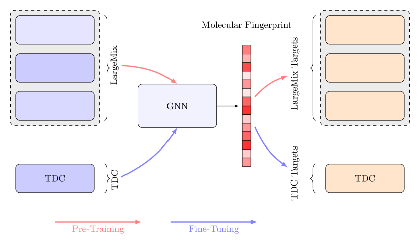
Figure 1: Workflow overview of the MiniMol pre-training and downstream task evaluation. MiniMol is pre-trained on the LargeMix datasets. Then MiniMol embeddings are used as molecular fingerprints for downstasks such as those in TDC.

Accurate prediction of molecular properties plays an essential role in many applications, including novel drug discovery (stokes_deep_2020; jin_deep_2021; wallach_atomnet_2015), efficient catalyst development (zitnick_introduction_2020), and materials design (reiser_graph_2022). Traditionally, Density Functional Theory (DFT) methods (nakata2017pubchemqc) accurately compute molecular properties by physics simulation, but are computationally demanding even for small molecules, and becomes intractable in large scale of biological systems (10.3389/fchem.2023.1106495). Consequently, deep learning methods such as Graph Neural Networks (GNNs) (masters2023gps++; gasteiger2019directional) and graph transformers (rampavsek2022recipe) have achieved significant success in molecular representation learning. This is demonstrated in the recent Open Graph Benchmark (OGB) Large Scale Challenge where on the PCQM4Mv2 dataset, deep learning models produce accurate approximations of DFT while being significantly faster (lu2023highly; masters2023gps++). In addition, by training on DFT calculations and biological tasks, ML models can predict complex biochemical properties not possible with DFT alone. Therefore, building foundation models that capture chemical and biological knowledge from large amounts of pre-training data and adapt it for a wide range of downstream low-data tasks is a promising next step.

Prior work on foundational models for molecular learning has typically adopted the common practices used in computer vision and natural language processing, aiming for large model capacity and pre-training dataset size. Molecular foundation models such as MolE (mendez-lucio_mole_2022), ChemBERTa-2 (ahmad_chemberta-2_2022) and Galactica (taylor_galactica_2022) directly receive SMILES strings (weininger1989smiles) of molecules as input. However, a number of equally valid SMILES strings can denote the same molecule thus SMILES string based models are unable to represent the symmetries underlying the molecular graphs. Therefore, large amounts of pre-training data and a large model capacity is required to properly learn these symmetries. Recently, ULTRA (galkin_2023_ultra), a foundational model for knowledge graphs, demonstrated that properly respecting the symmetries of the underlying data alleviates the need for large models in order to beat task-specific baselines. Specifically, ULTRA improves the state-of-the-art on a wide variety of knowledge graph reasoning tasks with only 177K parameters. Therefore, we leverage the permutation invariant property of GNNs to build a generally-capable and parameter-efficient foundation model for molecular fingerprinting.

In this work, we propose MiniMol, a parameter-efficient foundation model for molecular learning based on GNN backbone. MiniMol is pre-trained on the Graphium LargeMix dataset (beaini2023towards) with around 6 million molecules and 526 million data labels. The pre-training strategy of Graphium is multi-level and multi-task meaning that over 3300 sparsely defined tasks on both graph and node level are trained jointly. MiniMol demonstrates strong downstream task performance on the Therapeutic Data Commons (TDC) ADMET group (huang2021therapeutics). Figure 1 shows a simplified diagram of this idea. Our main contributions are as follows:

• In this work, we propose MiniMol, a parameter-efficient foundation model with a GINE backbone of 10 million parameters, pre-trained on around 3300 biological and quantum tasks on the graph and node level of molecules.

• We demonstrate that the molecular fingerprint from MiniMol is highly transferable to downstream tasks. On the TDC benchmark, the current state of the art for a single model applied to all tasks (a foundation model) is MolE, which achieves a mean rank of 5.4, when compared against the specialized per-task models on the leaderboard. MiniMol achieves a mean rank of 3.6 and outperforms MolE on 17 tasks.

• We conduct a thorough performance correlation analysis between the pre-training datasets and downstream tasks. We found that PCQM4M_G25 dataset often has a negative correlation with downstream tasks thus highlighting the importance of understanding the correlation between pre-training tasks and downstream tasks.

• MiniMol will be a public and open-sourced model for future research. With only 10% of the parameters of prior state-of-the-art, MiniMol offers strong downstream performance and lower compute requirement to adapt.

Reproducibility: We include the code and weight checkpoint for MiniMol needed to reproduce the experiments as supplementary materials.

2 Related Work

2.1 Molecular Fingerprints

Traditional molecular fingerprints such as Extended Connectivity Fingerprint (ECFP) (rogers2010extended), RDkit fingerprints (landrum2013rdkit) and MAP4 (capecchi2020one) are designed for molecular characterization, similarity searching, and structure-activity modelling, with wide applications in drug discovery. However, they encode the presence of particular substructures within the molecule and should be manually customized for specific applications. In addition, it is shown that different types of fingerprints perform better for specific categories of molecules. For example, substructure fingerprint (kim2021exploring) has the best performance on small molecules such as drugs while atom-pair fingerprints (awale2014atom) are best suited for large molecules such as peptides. Even SOTA fingerprints can suffer from embedding collisions due to how sub-structures are resolved (probst_reaction_2022). From large molecular datasets, foundation models aim to learn a universal and descriptive molecular representation as practical molecular fingerprints for downstream tasks. Our MiniMol model generates strong fingerprints for various tasks on the TDC benchmark as indicated by downstream task performance.

2.2 Foundational Models in ML.

In Natural Language Processing (NLP) and Computer Vision (CV), foundation models have achieved significant progress, especially for Large Language Models (LLMs) (achiam2023gpt). Foundation models are often pre-trained on a mixture of data across a wide range of tasks. Downstream tasks with low amounts of data can then be solved using low-resource, inexpensive fine-tuning (tian2023fine; borzunov2023distributed). Multi-modal datasets have been used with LLMs to align a single model representation across domains (team2023gemini; betker2023improving). In most areas, these general properties have typically been emergent from extremely large models.

2.3 Foundational Models in Molecular Learning.

Initial unsupervised transformer-based designs most closely replicate work in NLP (honda_smiles_2019; wang_smiles-bert_2019; honda_smiles_2019), representing molecules as SMILES strings (weininger_smiles_1988). These models leverage extremely large but low-fidelity unlabelled molecule datasets. Early FMs can achieve strong results on some small, out-of-domain tasks. However, generalizability to a wide variety of tasks remains limited (zhu_dual-view_2021; liu_towards_2023; mendez-lucio_mole_2022; luo_molfm_2023). Recent state-of-the-art in molecular property prediction employs geometric deep learning, often with an MPNN or Graph Transformer, trained with supervised labels of molecular properties (ying_transformers_2021; velickovic_graph_2017; dwivedi_generalization_2020). Recent work by  (masters_gps_2023) has shown promising potential for MPNN scaling in-depth and total parameters for predicting the quantum properties of molecules. Recent work COATI (kaufman_coati_2023) is based on SMILES and point clouds, utilizing a multi-modal encoder-decoder scheme designed for molecule regression tasks. Significantly, shoghi_molecules_2023 demonstrates the importance of multi-task pre-training on a range of length scales for low-resource fine-tuning and extracting learned representations for molecular property prediction (MPP). In this work, we use graph-based representations of molecules, which provide rich chemical and structural information. MiniMol is pre-trained on a large number of molecular properties of both quantum and biological tasks while demonstrating strong performance across many downstream tasks.

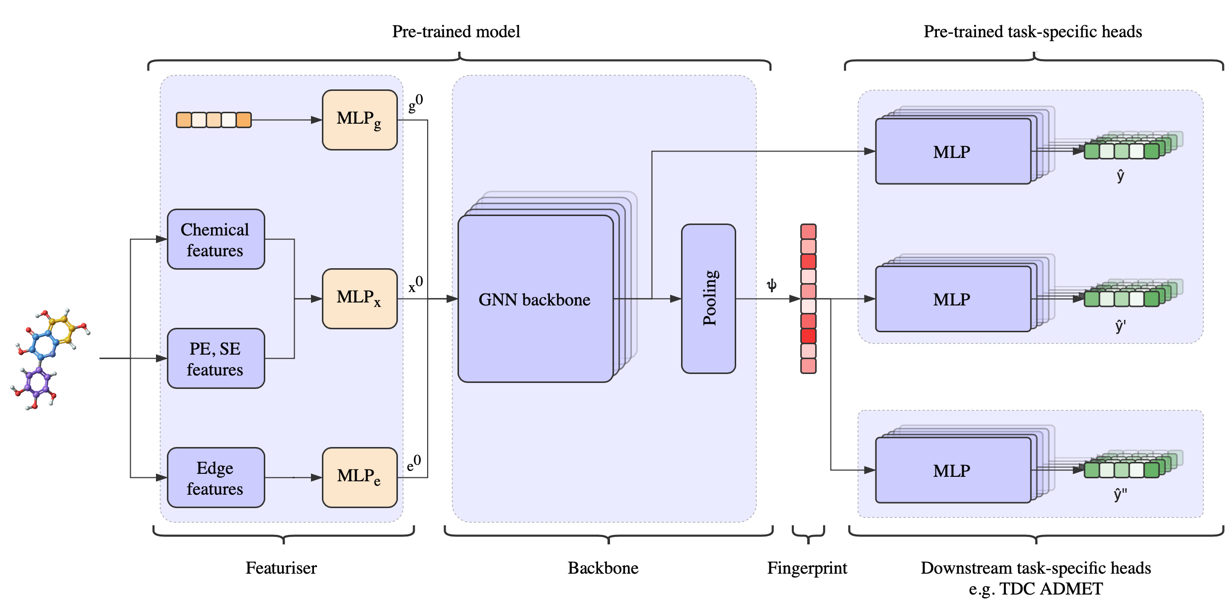
Figure 2: Schematic of the architecture of MiniMol. An example molecule is featurized in the first block. Node feature vectors are created by combining chemical features with positional and structural encodings, edge features are generated using RDKit and a random initial global vector is generated. Each initial vector is processed with a separate embedding MLP. The backbone of the model is a stack of MPNN layers, which output the molecular fingerprint $\psi$ after pooling. The pre-pooling output is used for pre-training on node-level tasks, in our case, PCQM4M_N4. The fingerprint $\psi$ is used either for pre-training multiple graph-level task heads or as an input to the downstream tasks, including the full set of ADMET tasks from the TDC benchmarks.

3 Method

Here, we present our architecture for pre-training on the LargeMix datasets (beaini_towards_2023), extracting fingerprints and subsequently fine-tuning to downstream tasks (see Fig. 2).

3.1 Molecular Representation

Each molecule is modelled as a graph $\mathcal{G}$ with $N$ nodes representing the atoms and $M$ edges representing the bonds. We denote the set of edges with $\mathcal{E}$. The atom and bond features are generated using RDKit, providing a set of categorical and floating values, and the atomic features are concatenated with positional and structural embeddings. From (masters_gps_2023; rampasek_recipe_2022) the Laplacian eigenvectors and eigenvalues, and the random walk probabilities, were found to be most beneficial. The input node feature vectors are the concatenation of these features

$$X^{0}=\left[X^{\mathrm{atom}}|X^{\mathrm{LapVec}}|X^{\mathrm{LapVal}}|X^{\mathrm{RW}}\right],$$

and edge features are the bond features $E^{0}=\left[E^{\mathrm{bond}}\right]$. A global node is added to each graph, providing an additional connection to every node. It was shown in (li_learning_2017)) that the global node dramatically improves graph-level representation. This acts both as routing between otherwise distant portions of the graph and as a readout node for the graph property. It is initialized with a random vector. Each of the nodes, edges, and global features are initially embedded into the model dimensions using a two-layer MLP each (eq 1 - 3).

$$x^{0}=\texttt{MLP}_{x}\left(X^{0}\right)\quad\in\mathbb{R}^{N\times d_{\mathrm{node}}}$$ (1)

$$e^{0}=\texttt{MLP}_{e}\left(E^{0}\right)\quad\in\mathbb{R}^{M\times d_{\mathrm{edge}}}$$ (2)

$$g^{0}=\texttt{MLP}_{g}(\texttt{rand}_{g}\left(0\right))\quad\in\mathbb{R}^{d_{\mathrm{global}}}$$ (3)

3.2 Model

Given the initial node, edge and graph embeddings we update them through multiple layers of message-passing to obtain final node embeddings

$$x^{\text{final}}=\texttt{GNN}(x^{0},e^{0},g^{0}),$$

where GNN is a chosen GNN backbone. As described later in Section 4, we try three different backbone GNNs, namely GCN (kipf2016semi), GINE (hu_strategies_2020; xu_how_2019) and MPNN++ (masters2023gps++). We briefly describe the different architectures here.

GCN

The GCN (kipf_semi-supervised_2016) incorporates only the node embeddings. Concretely, the $\ell$-th layer of a GCN is defined as

$$x_{i}^{\ell+1}=\sum_{j\in\mathcal{N}(i)\cup\{i\}}\dfrac{1}{\sqrt{d_{i}d_{j}}}x_{j}^{\ell},$$

where $\mathcal{N}(i)$ denotes the set of neighbors of $i$ and $d_{i}$ and $d_{j}$ denote the degree of nodes $i$ and $j$, respectively.

GINE

GINE is an extension of GIN (xu_how_2019) to additionally incorporate edge embeddings (hu_strategies_2020). Concretely, the $\ell$-th layer of GINE is defined as

$$x_{i}^{\ell+1}=\texttt{MLP}\Big{(}(1-\epsilon)\cdot x_{i}^{\ell}\sum_{j\in\mathcal{N}(i)}\texttt{ReLU}(x_{j}^{\ell}+e^{\ell}_{ij})\Big{)},$$

where $\epsilon$ is a learnable scalar. Compared to GCN, GINE is more expressive as it has the same expressive power for graph isomorphism test as the $1$-Weisfeiler-Leman algorithm (xu_how_2019). Further, GINE has been used previously for pre-training graph neural networks (hu_strategies_2020).

MPNN++

The Message Passing Neural Network (MPNN) module in (masters2023gps++) called MPNN++, is designed to incorporate and update node-, edge- and graph-level embeddings. The MPNN++ is a complex architecture as it aggregates messages from adjacent nodes, incident edges and global graph-level embeddings. In addition, the MPNN++ uses layer-wise skip connections for node-, edge- and graph-level embeddings; see LABEL:sec:mpnn_details for a detailed description of the MPNN++ layer. We include MPNN++ as a backbone in our experiments.

3.3 Pre-training

MiniMol is jointly pre-trained with many supervised tasks on both the graph and node levels. The total loss minimized during training is a summation of each of the pre-training tasks, accounting for label sparsity per molecule. There is a rich literature on how to combine losses for multi-task learning (crawshaw2020multi), although in this case, the tasks are a combination of regression and classification, meaning the losses are not naturally commensurate. The mean absolute error (MAE) loss is used for the PCQM dataset (N4 and G25 tasks), the binary cross-entropy (BCE) loss is used for the PCBA tasks, and the hybrid cross-entropy (HCE) loss from (beaini_towards_2023) is used for the L1000 datasets. Concretely, we compute the final loss $\mathcal{L}$ as

$$\mathcal{L}=\mathcal{L}_{\text{L1000}}+\mathcal{L}_{\text{PCBA}}+\mathcal{L}_{\text{N4}}+\frac{1}{k}\mathcal{L}_{\text{G25}}.$$

where $k$ is a scaling constant and we set $k=5$ to account for data imbalance on the G25 dataset (see more discussion in Section 4).

3.4 Downstream Fingerprinting

For downstream tasks, we generate the global embeddings of the final layer of MiniMol from a given molecule which is also referred to as molecular fingerprints. This is more compute efficient and easy to use when compared to fine-tuning the entire model from end-to-end. In addition, generating meaningful molecular fingerprints for downstream tasks is an important aspect of the foundation model of molecular learning.

More specifically, we first extract fingerprints for all unique molecules in a given downstream task and subsequently use the fingerprints as molecular representation to train a small Multilayer Perceptron (MLP) for making task-specific predictions. To generate the fingerprints from MiniMol, we compute the final node-, edge- and graph-level embeddings as described in Section 3.2 and subsequently obtain fingerprints by pooling the final node embeddings, e.g., via max pooling, obtaining

$$\psi=\sum_{i\in\mathcal{G}}x^{\text{final}}_{i}$$

for the fingerprint vector $\psi$.

There are several advantages of using molecular fingerprints for downstream tasks when compared to end-to-end fine-tuning. First, the above procedure allows a significantly more efficient way to train a model on low-data downstream tasks. Molecular fingerprints are pre-computed for a given set of molecules with a single forward pass from the model and then used for many downstream tasks or hyperparameter sweeps. Second, the downstream model is less likely to overfit when only the downstream MLP is trainable as there are fewer trainable parameters. Next, the use of molecular fingerprints for downstream tasks in this way matches existing workflows in the bio-chemistry domain increasing the practical utility of the method. Finally, as fingerprints are simply embedding vectors, practitioners are not required to access the architecture or weight of the pre-trained model thus only the expertise to train a task head (or MLP) is required.

4 Experimental Details

In our experiments, we pre-train MiniMol on LargeMix (beaini_towards_2023) for various GNN backbones and subsequently fine-tune to all 22 tasks in the ADMET Group of the TDC benchmark.

4.1 Pre-training

MiniMol uses the LargeMix datasets from (beaini_towards_2023) for pre-training, consisting of approximately 6M molecules and a total of 526M targets, which have been summarized in Table  1. The datasets are described below.

PCQM4M_G25_N4. This dataset contains 3.8M molecules from the PCQM dataset (hu2021ogb), from the OGB-LSC challenge. The dataset consists of quantum chemistry calculations for 25 molecular graph-level properties, and 4 node-level properties per atom, resulting in about 400M labelled data points.

PCBA. This dataset contains 1.5M molecules from the OGBG-PCBA dataset (hu2020open). This bioassay dataset, derived experimentally from high-throughput screening methods, details the impact of the molecules on living cells across 1328 sparse labels. This results in about 100M labelled data points.

L1000_VCAP and L1000_MCF7. These datasets contain 26k molecules from the L1000 dataset (subramanian2017next) which details the change to gene expression profiles and cellular processes when exposed to the molecules in the dataset across about 1000 labels and 26M data points.

Table 1: Overview of the datasets in LargeMix.

Dataset	# Molecules	# Labels	# Data Points	% of All Data Points
PCQM4M_G25	3.81M	25 (G)	93M	17%
PCQM4M_N4	3.81M	4 (N)	197.7M	37%
PCBA_132B	1.56M	1328 (G)	224.4M	41%
L1000_VCAP	15K	978 (G)	15M	3%
L1000_MCF7	12K	978 (G)	11M	2%

These diverse labels from fundamental quantum chemistry properties to macro-scale cellular impact encourage a single general representation of the molecule suitable for downstream tasks. The combined LargeMix contains multiple task labels per molecule. The datasets only partially overlap thus requiring the model to generalize across domains from sparse labels on molecules. Following (mendez-lucio_mole_2022), we filter out molecules with more than 100 heavy atoms. In addition, we remove molecules in the ADMET group test sets from our pre-training data to avoid potential leakage of test labels (7% of MCF7, 4% of VCAP, 0.6% of PCBA, 0.07% of PCQM4M_G25/N4). During pre-training we split the dataset into 92% training, 4% validation, and 4% test data.

To cover a range of GNN backbones with increasing complexity, we pre-train GCN, GINE, and finally MPNN++ models and subsequently evaluate their downstream performance on the TDC ADMET group datasets. Each model consists of 16 GNN layers with hidden dimensions adjusted such that all models have around 10M parameters. We train each model for 100 epochs using the Adam optimizer, with a maximum learning rate of $3e^{-4}$, 5 warm-up epochs and linear learning rate decay.

4.2 Benchmarking on TDC ADMET Group

Here, we describe the ADMET group of the TDC benchmark which we use to evaluate the downstream performance of MiniMol. The Therapeutics Data Commons (TDC) (huang2021therapeutics) is a platform designed to facilitate the assessment and development of AI methods in drug discovery. It particularly emphasizes identifying the most effective AI techniques for this purpose. Within TDC, the ADMET Benchmark Group specializes in single-instance prediction, offering a standardized suite of 22 datasets for molecular property prediction. These datasets vary in size, ranging from 475 to 13,130 molecules, and encompass tasks in both regression and classification. The datasets span a breadth of molecular properties, categorized into Absorption, Distribution, Metabolism, Excretion, and Toxicity. To ensure fair comparability, scaffold splits are employed, with 80% of data for training and 20% for testing.

A diverse array of models, including random forests, GNNs, and CNNs, are evaluated on these tasks. Their performance is showcased on the TDC leaderboard which includes various models trained with SMILES or other encoding strategies. To benchmark MiniMol, we first build an ensemble by training a distinct model on each fold in 5-fold cross-validation. While building the ensemble, the best epoch is selected based on validation loss, and to distinguish which ensemble to select for testing (e.g. while choosing one out of the sweep), the ensemble’s mean validation metric is used. Final test scores are derived from the top ensemble, with error bars reported from five trials (see Appendix LABEL:sec:ensembling_strategy for pseudo code). Table 5.1 presents the performance of three GNN architectures (GCN, GINE, MPNN++) across various datasets and two computational budgets for sweeping hyperparameters of the dataset-specific models. Since our fingerprinting approach permits fast evaluation of downstream predictors, we conduct extensive hyperparameter sweeping across all tasks (see Appendix LABEL:sec:hyperparameter_selection for more details about the hyperparameter selection). For CPU-only runs, training a downstream model only takes 1 to 10 minutes per model per dataset.

Table 2: Results on downstream evaluation of MiniMol (GINE) with max pooling on TDC ADMET benchmarks, and comparison to the TDC leaderboard and MolE. The rank is determined for each dataset individually, on a set of 7 scores, which include the test results from the TOP5 leaderboard, MolE and MiniMol. The best result is shown in green and the top three results are highlighted in purple.

—l—l—r—r—l—l—c—l—c— TDC Dataset Leaderboard Jan. 2024 MolE MiniMol (GINE)
Name Size Metric SOTA Result Result Rank Result Rank
Absorption Caco2 Wang 906 MAE ($\downarrow$) 0.276 $\pm$ .005 0.310 $\pm$ .010 6 0.324 $\pm$ .012 7
Bioavailability Ma 640 AUROC ($\uparrow$) 0.748 $\pm$ .033 0.654 $\pm$ .028 7 0.699 $\pm$ .008 6
Lipophilicity AZ 4,200 MAE ($\downarrow$) 0.467 $\pm$ .006 0.469 $\pm$ .009 3 0.455 $\pm$ .001 1
Solubility AqSolDB 9,982 MAE ($\downarrow$) 0.761 $\pm$ .025 0.792 $\pm$ .005 5 0.750 $\pm$ .012 1
HIA Hou 578 AUROC ($\uparrow$) 0.989 $\pm$ .001 0.963 $\pm$ .019 7 0.994 $\pm$ .003 1
Pgp Broccatelli 1,212 AUROC ($\uparrow$) 0.938 $\pm$ .002 0.915 $\pm$ .005 7 0.994 $\pm$ .002 1
Distrib. BBB Martins 1,975 AUROC ($\uparrow$) 0.920 $\pm$ .006 0.903 $\pm$ .005 7 0.923 $\pm$ .002 1
PPBR AZ 1,797 MAE ($\downarrow$) 7.526 $\pm$ .106 8.073 $\pm$ .335 6 7.807 $\pm$ .188 4
VDss Lombardo 1,130 Spearman ($\uparrow$) 0.713 $\pm$ .007 0.654 $\pm$ .031 3 0.570 $\pm$ .015 7
Metabolism CYP2C9 Veith 12,092 AUPRC ($\uparrow$) 0.859 $\pm$ .001 0.801 $\pm$ .003 5 0.819 $\pm$ .001 4
CYP2D6 Veith 13,130 AUPRC ($\uparrow$) 0.790 $\pm$ .001 0.682 $\pm$ .008 6 0.718 $\pm$ .003 5
CYP3A4 Veith 12,328 AUPRC ($\uparrow$) 0.916 $\pm$ .000 0.867 $\pm$ .003 7 0.878 $\pm$ .001 5
CYP2C9 Substrate 666 AUPRC ($\uparrow$) 0.441 $\pm$ .033 0.446 $\pm$ .062 2 0.481 $\pm$ .013 1
CYP2D6 Substrate 664 AUPRC ($\uparrow$) 0.736 $\pm$ .024 0.699 $\pm$ .018 7 0.726 $\pm$ .006 2
CYP3A4 Substrate 667 AUROC ($\uparrow$) 0.667 $\pm$ .019 0.670 $\pm$ .018 1 0.644 $\pm$ .006 6
Excret. Half Life Obach 667 Spearman ($\uparrow$) 0.576 $\pm$ .025 0.549 $\pm$ .024 4 0.493 $\pm$ .002 7
Clearance Hepatocyte 1,102 Spearman ($\uparrow$) 0.536 $\pm$ .020 0.381 $\pm$ .038 7 0.448 $\pm$ .006 4
Clearance Microsome 1,020 Spearman ($\uparrow$) 0.630 $\pm$ .010 0.607 $\pm$ .027 6 0.652 $\pm$ .007 1
Toxicity LD50 Zhu 7,385 MAE ($\downarrow$) 0.552 $\pm$ .009 0.823 $\pm$ .019 7 0.588 $\pm$ .010 3
hERG 648 AUROC ($\uparrow$) 0.880 $\pm$ .002 0.813 $\pm$ .009 7 0.849 $\pm$ .007 6
Ames 7,255 AUROC ($\uparrow$) 0.871 $\pm$ .002 0.883 $\pm$ .005 1 0.856 $\pm$ .001 5
DILI 475 AUROC ($\uparrow$) 0.925 $\pm$ .005 0.577 $\pm$ .021 7 0.944 $\pm$ .007 1
TDC Leaderboard Mean Rank: 5.4 3.6

5 Empirical Results

Here, we present our experimental results for both pre-training and fine-tuning on fingerprints.

5.1 Pre-training on LargeMix

We present our pre-training results for MiniMol with GCN, GINE and MPNN++ as backbone GNNs on LargeMix in Section 5.1. Here, we observe that pre-training performance is only marginally affected by the choice of the backbone GNN. Moreover, the pre-training performance of a given GNN backbone also varies with tasks. For example, on the graph- and node-level regression tasks of PCQM4M_G25 and PCQM4M_N4 the MPNN++ backbone performs consistently better while GINE performs best on the classification tasks of PCBA_1328. On L1000_VCAP we observe roughly comparable results across all metrics with a slight advantage of GINE in terms of AUROC. Finally, on L1000_MCF7, GCN and GINE are largely on par with the MPNN++ showing worse performance in terms of AUROC. Most importantly, no single backbone is superior to the other two. Next, we present our results of fine-tuning these models to the ADMET group benchmark of TDC using our fingerprinting approach.

Table 3: Results for GNN 10M baselines on LargeMix dataset. We report performance metrics on the test set for each dataset in LargeMix separately. The best scores per metric per dataset are marked in bold.

l—l—cccc   Model
Dataset Metric GCN GINE MPNN
Pcqm4m_g25 MAE $\downarrow$ 0.218 0.208 0.200
Pearson $\uparrow$ 0.884 0.889 0.892
$R^{2}$ $\uparrow$ 0.790 0.799 0.803
Pcqm4m_n4 MAE $\downarrow$ 0.025 0.022 0.021
Pearson $\uparrow$ 0.975 0.979 0.980
$R^{2}$ $\uparrow$ 0.952 0.959 0.961
Pcba_1328 CE $\downarrow$ 0.033 0.033 0.033
AUROC $\uparrow$ 0.777 0.784 0.782
AP $\uparrow$ 0.286 0.302 0.287
L1000_vcap CE $\downarrow$ 0.061 0.061 0.061
AUROC $\uparrow$ 0.500 0.514 0.500
AP $\uparrow$ 0.504 0.504 0.506
L1000_mcf7 CE $\downarrow$ 0.059 0.058 0.059
AUROC $\uparrow$ 0.533 0.531 0.519
AP $\uparrow$ 0.513 0.516 0.514

Table 4: The effect of specific GNN architectures in the backbone of the fingerprinting model on the downstream performance. The rank is determined for each dataset individually, on a set of 7 scores, which include the test results from the TOP5 TDC leaderboard, MolE and MiniMol. Here, all models used sum pooling, whereas our best model uses max pooling.

@r—c—c—c@ MiniMol backbone Mean Rank # Top1 Results # Top3 Results
MPNN++ 4.8 3 6
GCN 4.4 4 8
GINE 3.9 5 10

5.2 Downstream performance on TDC

Here, we present our fine-tuning results on the ADMET group datasets of TDC; see Section 5.1 for a comparison of different backbone GNNs in terms of downstream performance. GINE demonstrates a significant empirical advantage as the GNN backbone for downstream tasks. Thus, in Section 4.2, we compare MiniMol (GINE), to the TDC leaderboard and the current state-of-the-art, MolE (mendez-lucio_mole_2022). MiniMol with GINE backbone, achieves top 1 performance on 8 tasks, setting a new state-of-the-art on these datasets. Moreover, MiniMol (GINE) achieves top-3 performance on 10 tasks. Therefore, MiniMol (GINE) is shown to be a versatile model across a wide range of tasks, competing with or exceeding the performance of the best task-specialized architectures. We report TDC leaderboard results up until January 2024. In addition, MiniMol (GINE) outperforms MolE on 17 datasets, indicating that with only 10% of the parameters, our MiniMol approach is favourable to MolE in downstream performance across many molecular tasks. For our best model, we explored different pooling methods, see Appendix  LABEL:sec:pooling_experiments.

In Table  5, we compare MiniMol to other fingerprinting methods using the same evaluation downstream adaptation method as ours, so the only difference is the quality of generated fingerprints.

Table 5: Comparison of MiniMol to other molecular fingerprinting models using the same evaluation method as ours, including ensembles.

Model	Mean rank	$>$MoIE	TOP1	TOP3
MiniMol	3.6	17	8	10
AGBT (chen2021algebraic)	5.7	10	1	4
MolFormer (ross2022large)	5.7	7	0	4
BET (chen2021extracting)	6.1	7	1	2

Table 6: Correlation analysis (Spearman’s rho) between pre-training validation and downstream performance. The green color indicates positive correlation , and red a negative correlation. Results with a p-value over 10% are blank. See §LABEL:sec:correlation for discussion.

l—l—c—c—c—c—c—c—c—c—c—c Dataset Metric Overall Loss L1000_MCF L1000_VCAP PCBA PCQM4M_G25 PCQM4M_N4

Loss AUROC Loss AUROC Loss AUROC Loss MAE Loss (MAE)
Caco2 Wang MAE 0.590 0.651 0.762 0.718
Bioavailability Ma AUROC 0.397
Lipophilicity AZ MAE 0.459 0.561 0.568 0.539 0.683 0.627 -0.389
Solubility AqSolDB MAE 0.434 0.472 0.588 0.7 0.739 0.704
HIA Hou AUROC 0.427 0.489 0.603 0.382 0.548 0.768 0.645 -0.337
Pgp Broccatelli AUROC 0.444 0.577 0.361 0.497 -0.387
BBB Martins AUROC 0.634 0.436 0.583 0.378 0.481 0.483 0.364 -0.492
PPBR AZ MAE 0.476 0.436
VDss Lombardo Spearman 0.408 0.343 0.351
CYP2C9 Veith AUPRC 0.432 0.649 0.711 0.747 0.829 0.557 0.551
CYP2D6 Veith AUPRC 0.566 0.641 0.487 0.624 0.704 0.616 0.585
CYP3A4 Veith AUPRC 0.523 0.649 0.713 0.72 0.818 0.584 0.608
CYP2C9 Substrate AUPRC 0.523 0.558 -0.377 -0.445 -0.566 -0.586
CYP2D6 Substrate AUPRC
CYP3A4 Substrate AUROC 0.409 0.468
Half Life Obach Spearman 0.503 0.671 0.498
Clearance Hepatocyte Spearman 0.374
Clearance Microsome Spearman 0.599 0.496
LD50 Zhu MAE 0.501 0.543 0.522 0.586 0.617 0.339 0.342
hERG AUROC 0.57 0.42 0.453
AMES AUROC 0.791 0.591 0.486 0.629 0.643 0.604 -0.628 0.528
DILI AUROC 0.376 0.49 0.416 0.567 0.454
Sum 5.622 4.883 6.496 2.269 7.959 9.712 7.749 2.499 -2.232 2.028