Importance of Disjoint Sampling in Conventional and Transformer Models for Hyperspectral Image Classification

Abstract

Disjoint sampling is critical for rigorous and unbiased evaluation of state-of-the-art (SOTA) models. When training, validation, and test sets overlap or share data, it introduces a bias that inflates performance metrics and prevents accurate assessment of a model’s true ability to generalize to new examples. This paper presents an innovative disjoint sampling approach for training SOTA models on Hyperspectral image classification (HSIC) tasks. By separating training, validation, and test data without overlap, the proposed method facilitates a fairer evaluation of how well a model can classify pixels it was not exposed to during training or validation. Experiments demonstrate the approach significantly improves a model’s generalization compared to alternatives that include training and validation data in test data. By eliminating data leakage between sets, disjoint sampling provides reliable metrics for benchmarking progress in HSIC. Researchers can have confidence that reported performance truly reflects a model’s capabilities for classifying new scenes, not just memorized pixels. This rigorous methodology is critical for advancing SOTA models and their real-world application to large-scale land mapping with Hyperspectral sensors. The source code is be available at https://github.com/mahmad00/Disjoint-Sampling-for-Hyperspectral-Image-Classification.

I Introduction

Hyperspectral Image Classification (HSIC) plays a pivotal role in various domains such as remote sensing [1], earth observation [2], urban planning [3], agriculture [4], forestry [5], target/object detection [6], mineral exploration [7], environmental monitoring [8, 9], climate change [10] food processing [11, 12], bakery products [13], bloodstain identification [14, 15], and meat processing [16, 17]. The rich spectral information provided by HSIs, often spanning hundreds of narrow bands, presents both challenges and opportunities for effective classification [18]. In recent years, Convolutional Neural Networks (CNNs) [19], Graph-based CNNs (GCNNs) [20, 21] and Transformers [22, 23] models have demonstrated remarkable success in various computer vision tasks, prompting researchers to explore their potential in HSI analysis. However, the computational complexity and memory requirements associated with processing the entire hyperspectral (HS) data pose significant challenges [24]. In this context, this work focuses on the importance of disjoint sampling in training, validation, and testing such models for HSIC.

Random sampling for data splitting can lead to several issues. It can result in non-representative training, validation, and test sets, causing models to overfit or underfit the data. Different random splits produce inconsistent results, making it hard to draw meaningful conclusions [25, 26]. Random sampling offers no control over data distribution, introducing bias in imbalanced datasets. It hinders the reproducibility of experimental results and limits the exploration of data relationships. Disjoint sampling is an important yet often overlooked consideration when evaluating spatial-spectral classification models. As demonstrated by the works [21, 27, 28, 29, 30, 1, 31], traditional evaluations using overlapping training and test samples can lead to biased results and unfair assessments of model performance. Their work presents a systematic evaluation of conventional and 3D convolutional neural network (CNN) models trained on disjoint HS samples and evaluated on disjoint validation sets. In addition to reporting overall accuracy, they analyze statistical measures like precision, recall, and F1-score to better validate the model’s generalized performance. Their results show that models trained on disjoint samples generalize better to unseen data, compared to models trained on the entire dataset. Their findings highlight the importance and feasibility of using disjoint sampling approaches to robustly evaluate conventional and 3D CNN models, which have large capacities and could overfit standard evaluations without adequate disjoint training and testing.

Even though these methodologies [21, 28, 30] meticulously employ disjoint sets for training, validation, and testing their models, there’s a notable inconsistency in their approach when it comes to generating land-cover maps. Specifically, many of these methods deviate from the disjoint sampling principle by utilizing the entire HSI dataset for land-cover classification (Thematic Maps). This practice introduces a conflict between the reported accuracy and the methodology employed. To address this inconsistency, it is essential to advocate for the use of disjoint test sets exclusively for generating land-cover maps. By doing so, the evaluation process aligns more closely with the principles of unbiased model assessment. It ensures that the model is confronted with truly unseen data during the map generation phase, fostering a more accurate representation of its real-world performance. This refined approach contributes to the transparency and reliability of reported accuracies, ultimately enhancing the credibility of land-cover mapping results in hyperspectral imaging studies.

Moreover, disjoint sampling is essential for training and evaluating deep models in HSI-based land cover classification. This method involves carefully selecting diverse and representative samples from various regions, land cover types, and environmental conditions to overcome biased or non-representative training data limitations [32]. It ensures the model learns robust features, enhancing classification performance and adaptability to unseen data. Additionally, disjoint sampling facilitates fair and accurate model evaluation by keeping training, validation, and testing samples separate [33]. Furthermore, it enhances model interpretability as diverse samples help the model learn distinctive spectral characteristics associated with different land cover classes. This interpretability is crucial for building trust in the model’s predictions and ensuring successful deployment in real-world applications. Furthermore, disjoint sampling is crucial in training SOTA models for HSIC, notably for CNN and Spatial-Spectral Transformer-based models. It enhances generalization, ensures fair evaluation, and enables result interpretability. This sampling strategy empowers researchers to maximize the potential of HS data, creating accurate models for diverse applications. The use of disjoint training, validation, and test samples is imperative in HSIC for various reasons, such as:

Unbiased Evaluation and Hyperparameter Tuning: It is crucial to evaluate HSIC models using completely separate and disjoint data for training, validation, and testing in order to properly assess a model’s true ability to generalize to new unknown examples [27]. The validation set plays a critical role in systematically developing a customized model for optimal performance. During training, numerous hyperparameters shape characteristics such as architecture and complexity but are not informed by the training data, necessitating impartial evaluation of candidate models to select the best-performing configuration. Through an iterative process of training models with varying hyperparameters on the training set and then evaluating their generalization ability solely on the held-out validation set, the ideal hyperparameter values producing a model specifically tailored to the nuances captured in the full dataset can be identified. By maintaining a rigorous separation of samples, we obtain an honest measure of the model’s predictive power on genuinely new observations and can be confident that it has learned to generalize, not memorize, enabling accurate classification of instances well beyond the initial data used to build the model [1].

Preventing Data Leakage and Mitigating Overfitting: Maintaining disjoint samples for training, validation, and testing is crucial to obtaining an accurate evaluation of a model’s true generalization performance [21, 33]. Utilizing disjoint subsets of the data for each stage of model development plays a critical role in enhancing generalization performance. By training on distinct partitions in an iterative fashion, the model is compelled to deduce underlying patterns common across diverse examples rather than potentially noisome idiosyncrasies within a single fixed training sample [34, 35]. This discourages the memorization of spurious characteristics unique to a single snapshot of data and instead cultivates the ability to accurately handle a broader array of presentations, both seen and novel. In this paper, we have made the following contributions:

1. We present a novel approach for generating disjoint train, validation, and test splits for HSIC. By ensuring the disjoint splits, the approach eliminates data leakage between subsets which can bias performance evaluations.

2. The proposed technique also provides a practical implementation for creating disjoint train, validation, and test splits from ground truth data in HSIC. This allows researchers to obtain unbiased performance evaluations and reliable comparisons between HSIC models.

3. By offering a standardized approach for creating evaluation splits, the proposed technique enhances the reproducibility and transparency of HSIC research. It fosters a more rigorous and standardized evaluation of classification models in the HSI domain.

In the subsequent section, we present our proposed methodology. Section III provides the experimental results and their discussion, and Section IV concludes the paper.

II Proposed Methodology

Let’s consider HSI data composed of $B$ spectral bands, each with a spatial resolution of $M\times N$ pixels. The HSI data cube, denoted as $X\in\mathbb{R}^{(M\times N\times B)}$, is initially partitioned into overlapping 3D patches [23, 36]. Each patch is centered at a spatial location $(\alpha,\beta)$ and covers a spatial extent of $S\times S$ pixels across all $B$ bands. The total number of 3D patches ($m$) extracted from $X$ (i.e., $X\in\mathbb{R}^{(S\times S\times B)}$) is given by $(M-S+1)\times(N-S+1)$. A patch located at $(\alpha,\beta)$ is represented as $P_{\alpha,\beta}$ and spans spatially from $\alpha-\frac{S-1}{2}$ to $\alpha+\frac{S-1}{2}$ in width and $\beta-\frac{S-1}{2}$ to $\beta+\frac{S-1}{2}$ in height. The labeling of these patches is determined by the label assigned to the central pixel within each patch as described in Algorithm 1.

Input : HSI, GT, WS

1 r, c, b $\leftarrow$ dimensions of HSI;

2 margin $\leftarrow$ WS / 2;

3 Pad $\leftarrow$ pad HSI with zeros on all sides;

4 Cubes $\leftarrow$ create an array of size (r $\times$ c, WS, WS, b);

5 Labels $\leftarrow$ create an array of size (r $\times$ c) ;

6 patchIndex $\leftarrow$ 0;

7 for rr $\leftarrow$ margin to rr + margin do

8       for cc $\leftarrow$ margin to cc + margin do

9             cube $\leftarrow$ select a sub-array from Pad Cubes[patchIndex, :, :, :] $\leftarrow$ cube;

10             Labels[patchIndex] $\leftarrow$ GT[rr - margin, cc - margin];

11             patchIndex $\leftarrow$ patchIndex + 1;

12            

13      

14return Cubes, Labels;

Algorithm 1 Create 3D HSI Patches

Figure 1: The HSI cube is initially divided into overlapping 3D patches, as described in Algorithm 1. Each patch is centered at a spatial point and covers a $WS\times WS$ pixel extent across all spectral bands. These patches are then used in Algorithm 2 to create a disjoint train, validation, and test splits based on the geographical locations of the HSI samples. The selected samples are inputted into various models for feature learning and optimization. The processed features are subsequently passed through a fully connected layer for classification, and the softmax function is applied to generate class probability distributions. These distributions are used to generate the final ground truth maps for the disjoint validation, disjoint test, and full HSI test sets.

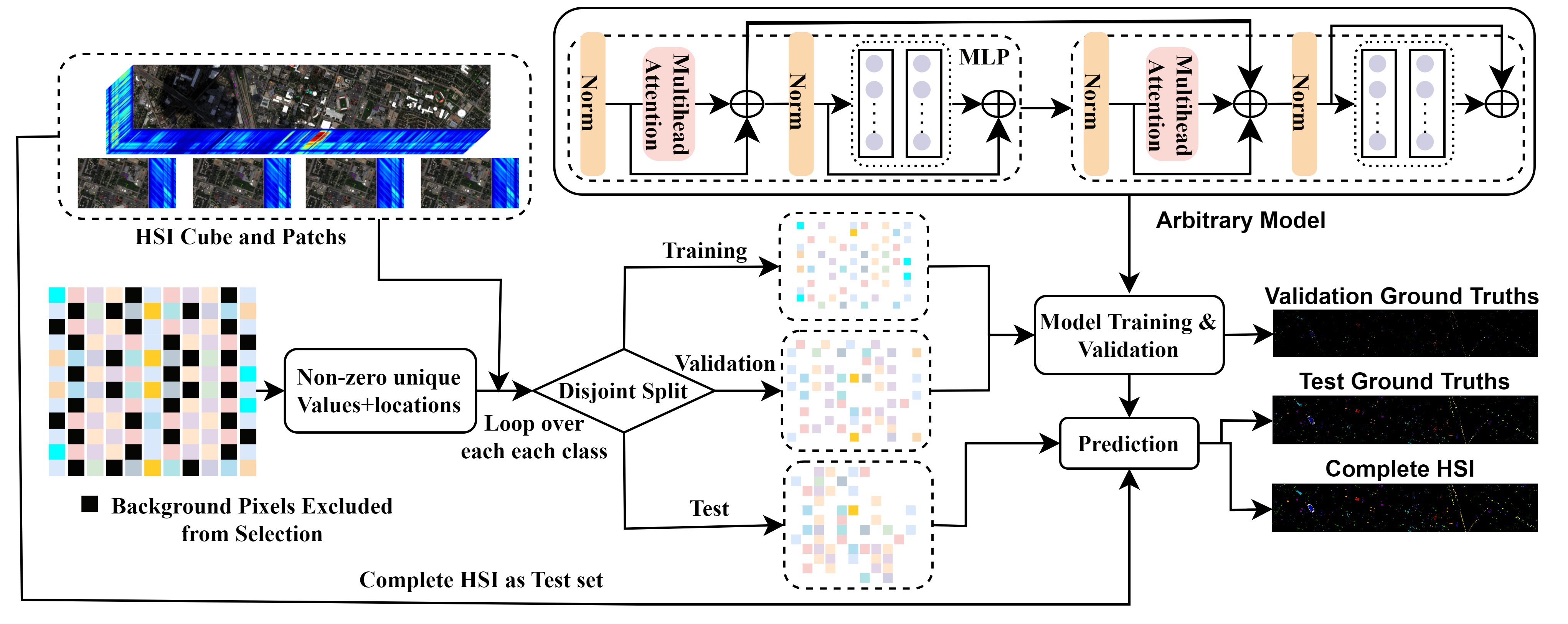
The 3D patches extracted from the HSI are used to generate separate training, validation, and test sets using the proposed splitting algorithm. The key algorithm, titled ”Disjoint Train, Validation, and Test Split”, handles dividing the HSI data into the respective portions. It takes the ground truth labels (GT) and ratios for the test and validation sets (teRatio and vrRatio) as inputs. The unique values in the GT labels and their frequency counts are identified, excluding zeros. An iterative process is then used to create disjoint training, validation, and test sets based on these unique values and their indices. The resulting indices are utilized to extract and organize the corresponding hyperspectral cubes and labels for each set. This ensures the subsets are separate while maintaining the integrity of spectral classes during model training and evaluation. The algorithm outputs the training, validation, and test samples along with their matching labels. This partitioning approach contributes to the robustness and reliability of the subsequent analysis.

Input : GT, p, m

1 flattened $\leftarrow$ GT.flatten();

2 unique $\leftarrow$ np.unique(flattened);

3 nonzero_indices $\leftarrow$ np.where(unique $\neq$ 0)[0];

4 unique $\leftarrow$ unique[nonzero_indices];

5 TrInd, VaInd, TeInd $\leftarrow$ [], [], [];

6 for value $\leftarrow$ unique do

7       C_ind $\leftarrow$ np.where(flattened == value)[0];

8       Tr_ind, Te_ind $\leftarrow$ train_test_split(C_ind, p);

9       Tr_ind, V_ind $\leftarrow$ train_test_split(Tr_ind, m);

10       TrInd.extend(Tr_ind);

11       VaInd.extend(V_ind);

12       TeInd.extend(Te_ind);

13      

Algorithm 2 Disjoint Train, Validation, and Test Split

Let us consider that $n$, $m$, and $p$ represent the finite numbers of labeled training, validation, and test samples, respectively, selected from $X$ (HSI dataset) to form the training set $D_{TR}={(x_{i},y_{i})}_{i=1}^{n}$ and the validation set $D_{V}={(x_{i},y_{i})}_{i=1}^{m}$. The remaining samples constitute the test set $D_{TE}={(x_{i},y_{i})}_{i=1}^{p}$. It is important to note that the intersection of the training set, validation set, and test set, denoted as $D_{TR}\cap D_{V}\cap D_{TE}$, is an empty set ($\phi$), ensuring the distinctiveness of the samples in each set as shown in Algorithm 2 and Figure 1.

III Experimental Results and Discussion

III-A Experimental Datasets

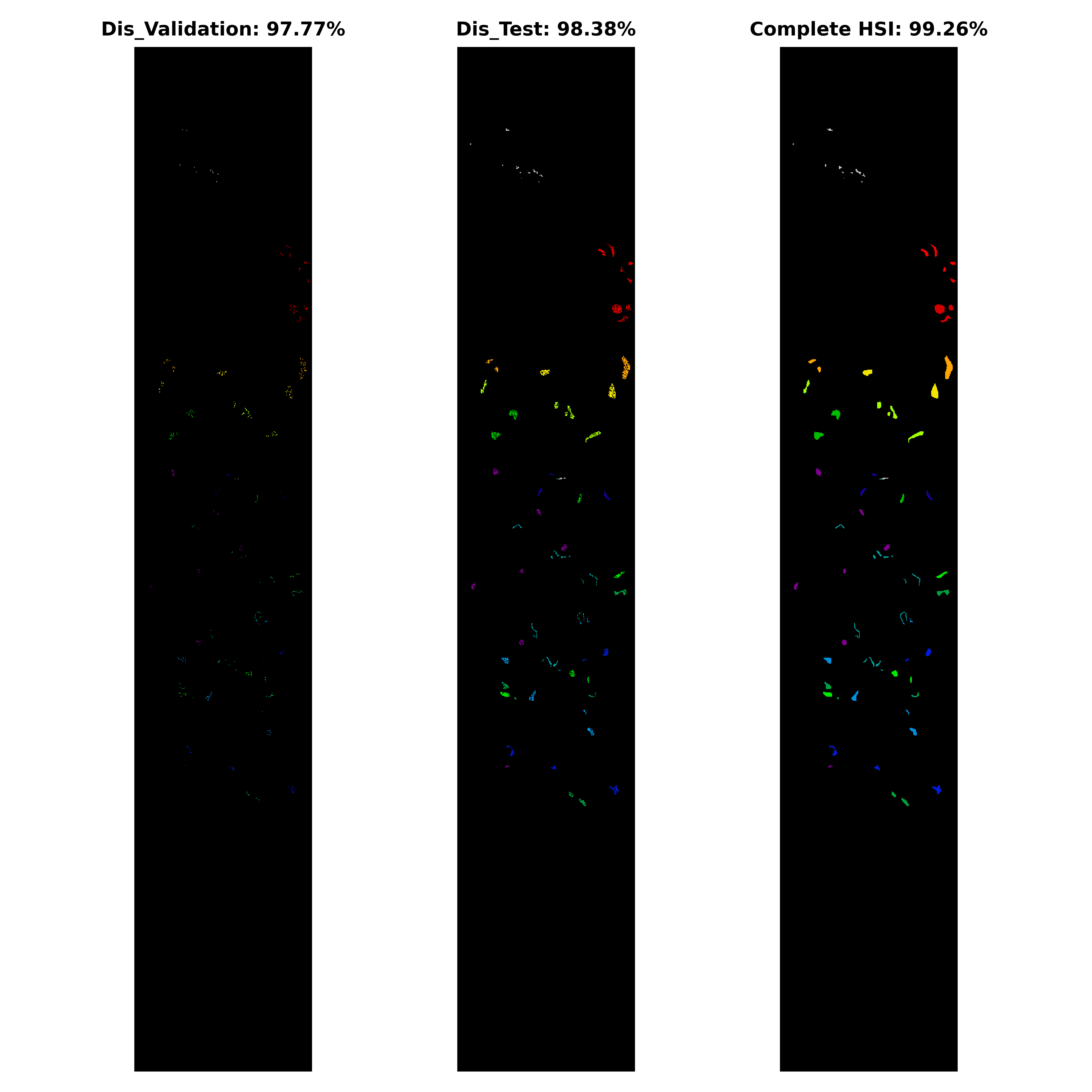
In order to further highlight the importance and the proposed procedure of disjoint sampling in HSIC, the following datasets are used. The University of Houston: The University of Houston HSI dataset consists of 144 spectral bands spanning wavelengths from 380 nm to 1050 nm, the dataset encompasses an imaged spatial region measuring 349 x 1905 pixels at a resolution of 2.5 meters per pixel. Additionally, the dataset annotates 15 labeled classes pertaining to urban land use and land cover types. The disjoint train, validation, and test samples are presented in Table I and Figure 2.

TABLE I: University of Houston Dataset: Disjoint sets of training (Tr), validation (Va), and test (Te) samples were chosen, with their geographical locations (Excluding background samples) illustrated in Figure 2, to train various SOTA models.

Class	Tr	Va	Te	Class	Tr	Va	Te
Healthy grass	75	300	876	Road	75	300	877
Stressed grass	75	301	878	Highway	73	295	859
Synthetic grass	41	168	488	Railway	74	296	865
Trees	74	299	871	Parking Lot 1	73	296	864
Soil	74	298	870	Parking Lot 2	28	112	329
Water	19	78	228	Tennis Court	25	103	300
Residential	76	304	888	Running Track	39	159	462
Commercial	74	299	871	-	-	-	-

Figure 2: University of Houston Dataset: Geographical locations of the disjoint train, validation, and test samples presented in Table I.

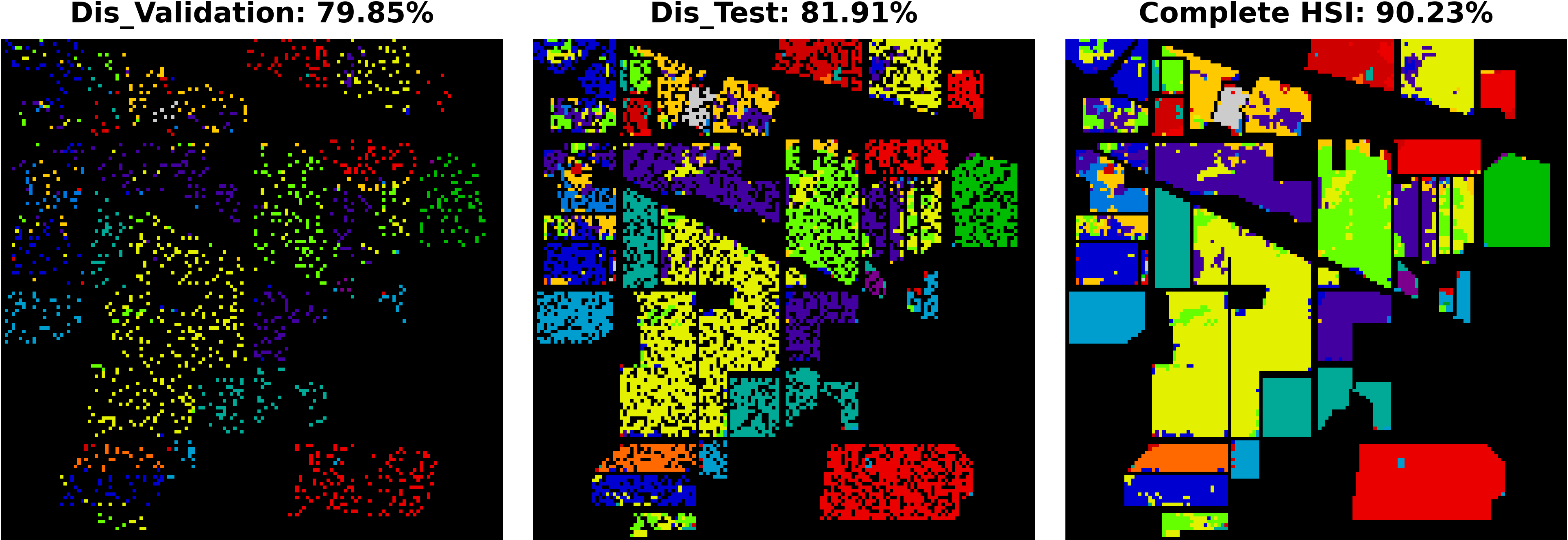
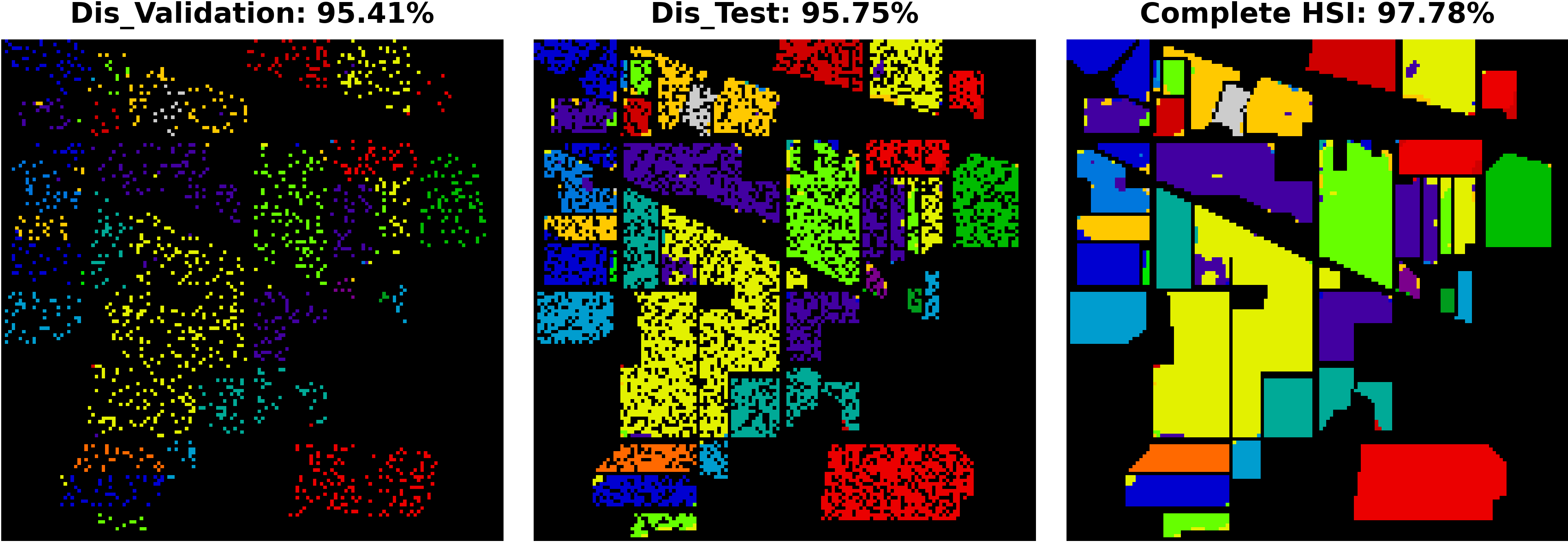
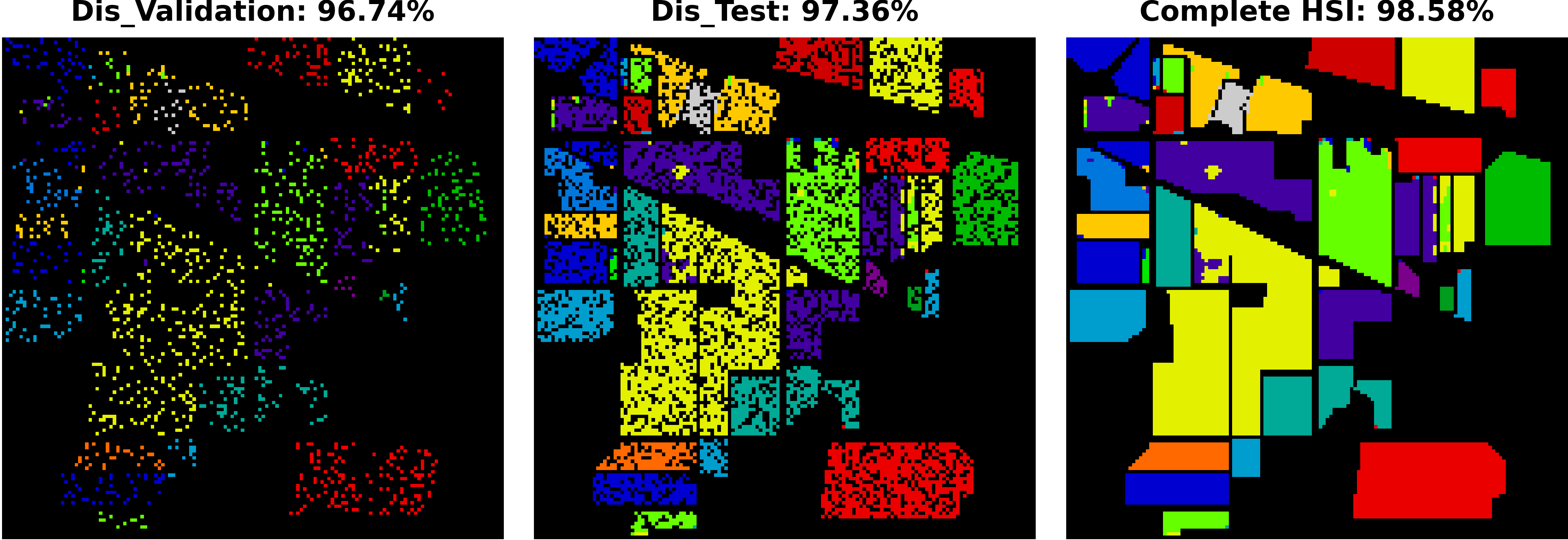
Indian Pines: The Indian Pines dataset was collected by the Airborne Visible/Infrared Imaging Spectrometer (AVIRIS) over an agricultural site in Northwestern Indiana. It consists of 145 x 145 pixels with spectral information across 224 narrow bands ranging from 0.4 to 2.5 micrometers. The major land cover classes in the dataset included agricultural land, forest, highways, rail lines, low-density housing, and built structures separated by smaller roads. Crops such as corn and soybeans covered less than 5% of typical growing areas as the June image showed early stages of development. Ground truths designate 16 non-mutually exclusive classes. The number of bands was reduced to 200 by removing wavelengths associated with water absorption. The disjoint train, validation, and test samples are presented in Table II and Figure 3.

TABLE II: Indian Pines Dataset: Disjoint sets of training (Tr), validation (Va), and test (Te) samples were chosen, with their geographical locations (Excluding background samples) illustrated in Figure 3, to train various SOTA models.

Class	Tr	Va	Te	Class	Tr	Va	Te
Alfalfa	6	7	33	Oats	3	3	14
Corn-notill	214	214	1000	Soybean-notill	145	146	681
Corn-mintill	124	125	581	Soybean-mintill	368	368	1719
Corn	35	36	166	Soybean-clean	88	89	416
Grass-pasture	72	72	339	Wheat	30	31	144
Grass-trees	109	110	511	Woods	189	190	886
Grass-mowed	4	4	20	Buildings	57	58	271
Hay-windrowed	71	72	335	Stone-Steel	13	14	66

Figure 3: Indian Pines: Geographical locations of the disjoint train, validation, and test samples presented in Table II.

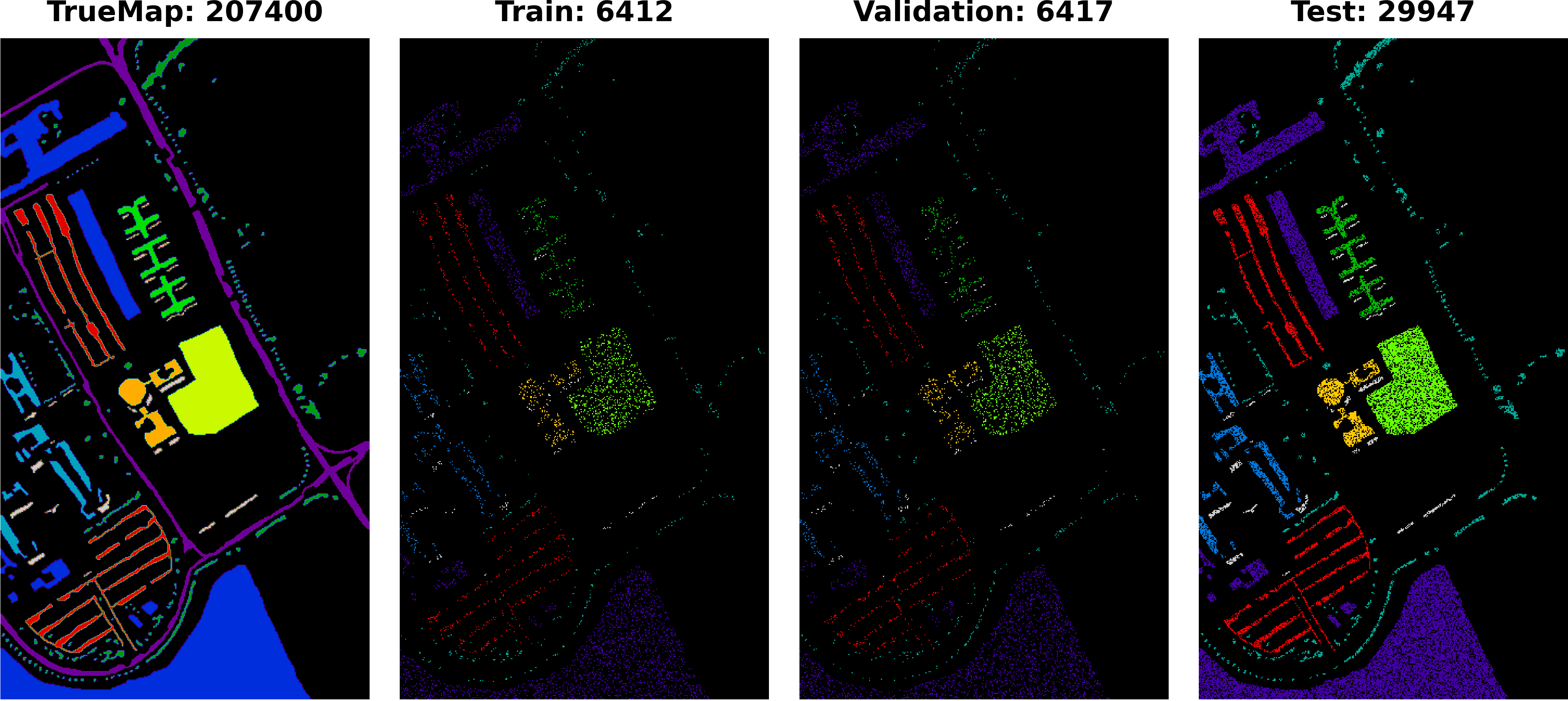
Pavia University: The Pavia University HSI dataset was captured using the reflective optics system imaging spectrometer, this dataset consists of an image with 610×340 pixels and 115 spectral bands. It has 9 classes of urban materials - including asphalt, meadows, gravel, trees, metal sheets, bare soil, bitumen, brick, and shadows - comprising 42,776 labeled samples in total. The disjoint train, validation, and test samples are presented in Table III and Figure 4.

TABLE III: Pavia University Dataset: Disjoint sets of training (Tr), validation (Va), and test (Te) samples were chosen, with their geographical locations (Excluding background samples) illustrated in Figure 4, to train various SOTA models.

Class	Tr	Va	Te	Class	Tr	Va	Te
Asphalt	994	995	4642	Soil	754	754	3521
Meadows	2797	2797	13055	Bitumen	199	200	931
Gravel	314	315	1470	Bricks	552	552	2578
Trees	459	460	2145	Shadows	142	142	663
Painted	201	202	942	-	-	-	-

Figure 4: Pavia University Dataset: Geographical locations of the disjoint train, validation, and test samples presented in Table III.

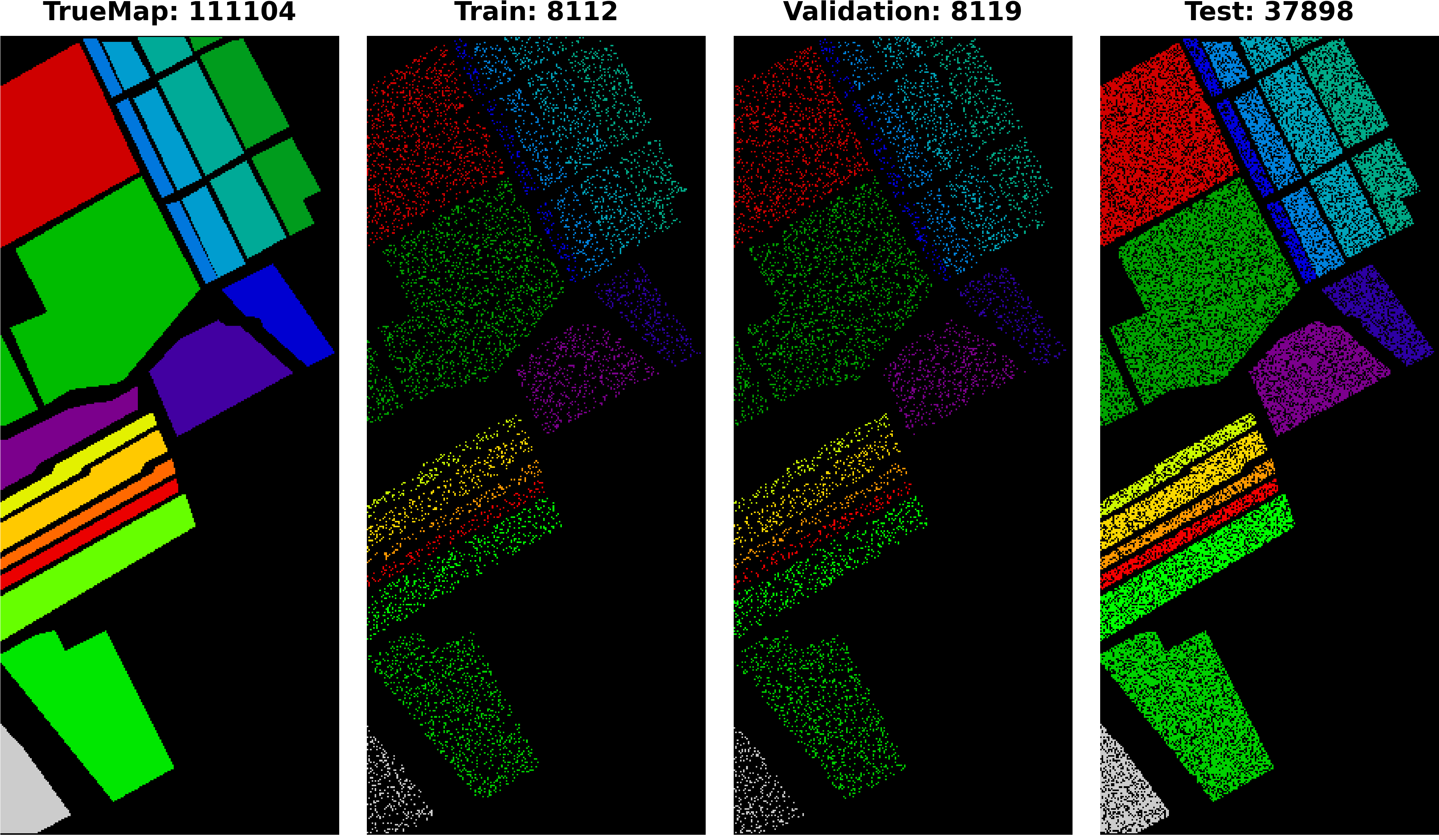
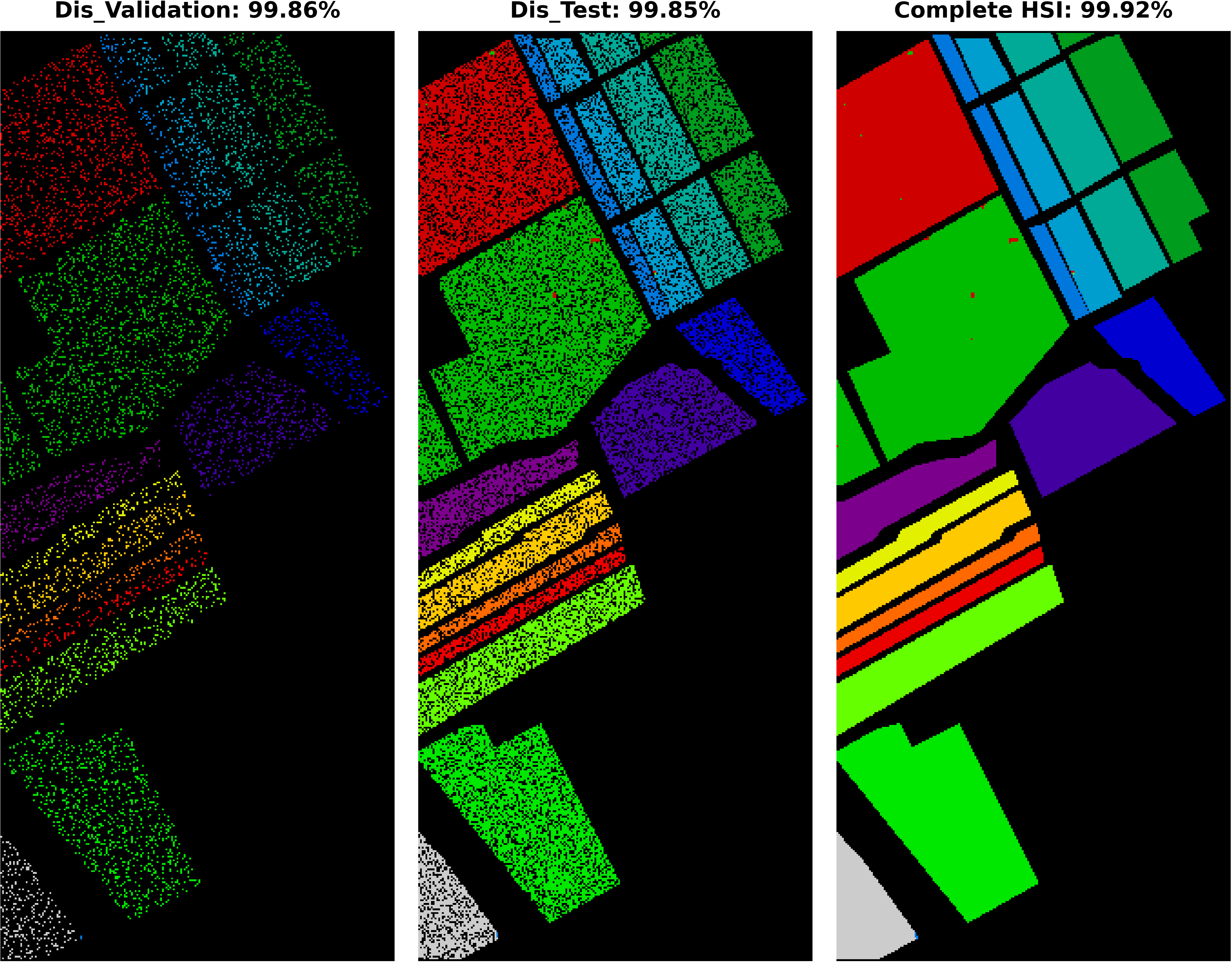
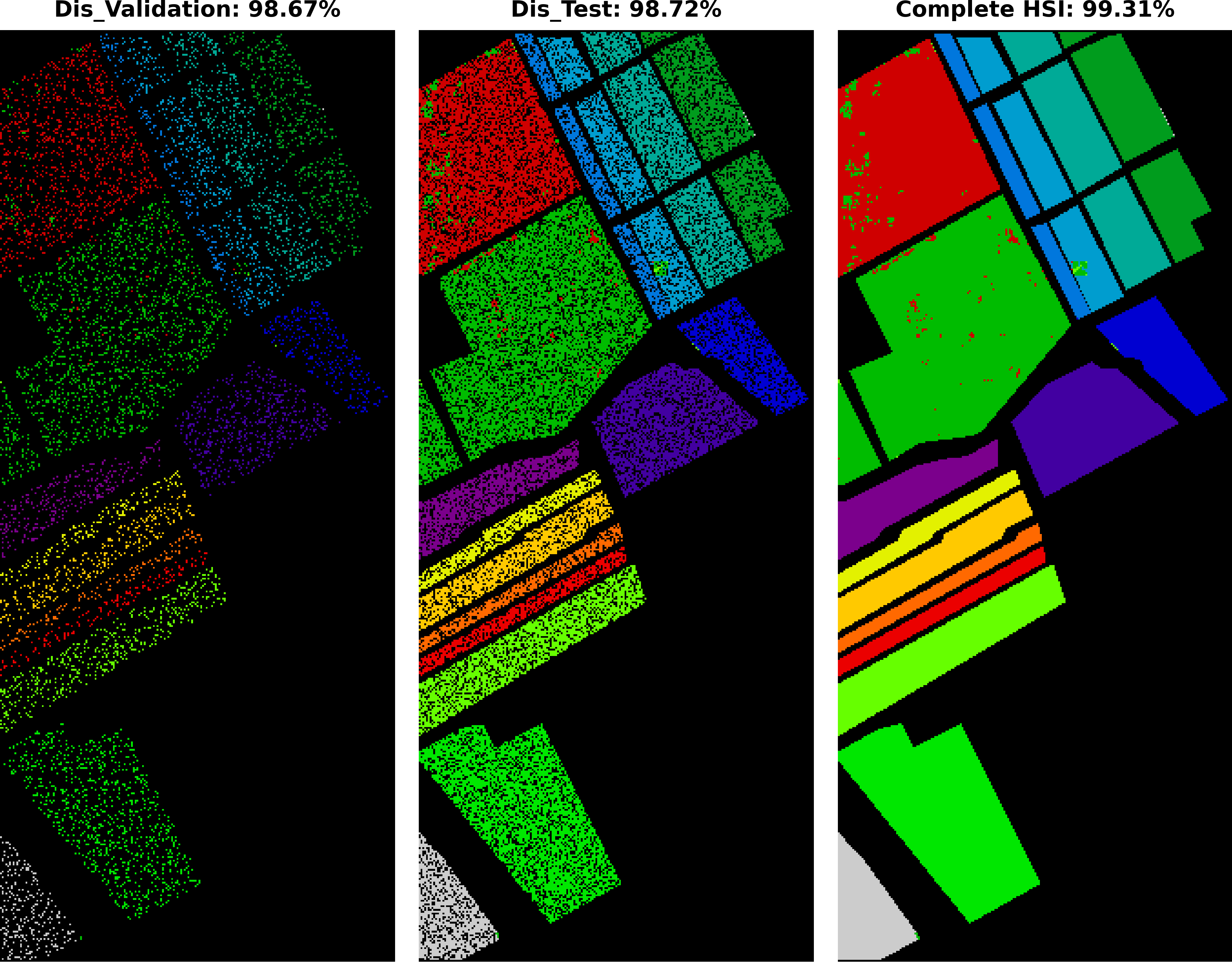
Salinas: The Salinas HSI dataset is collected using the 224-band AVIRIS sensor over Salinas Valley, California, this dataset is characterized by high spatial resolution at 3.7 meters per pixel. The study area encompasses 512 lines by 217 samples after removing 20 bands obscured by water absorption. Land cover types within the dataset include vegetables, bare soils, and vineyard fields. The Salinas ground truth annotates 16 classes. The disjoint train, validation, and test samples are presented in Table IV and Figure 5.

TABLE IV: Salinas Dataset: Disjoint sets of training (Tr), validation (Va), and test (Te) samples were chosen, with their geographical locations (Excluding background samples) illustrated in Figure 5, to train various SOTA models.

Class	Tr	Va	Te	Class	Tr	Va	Te
Weeds 1	301	301	1407	Soil vinyard develop	930	930	4343
Weeds 2	558	559	2609	Corn Weeds	491	492	2295
Fallow	296	296	1384	Lettuce 4wk	160	160	748
Fallow rough plow	209	209	976	Lettuce 5wk	289	289	1349
Fallow smooth	401	402	1875	Lettuce 6wk	137	137	642
Stubble	593	594	2772	Lettuce 7wk	160	161	749
Celery	536	537	2506	Vinyard untrained	1090	1090	5088
Grapes untrained	1690	1691	7890	Vinyard trellis	271	271	1265

Figure 5: Salinas Dataset: Geographical locations of the disjoint train, validation, and test samples presented in Table IV.

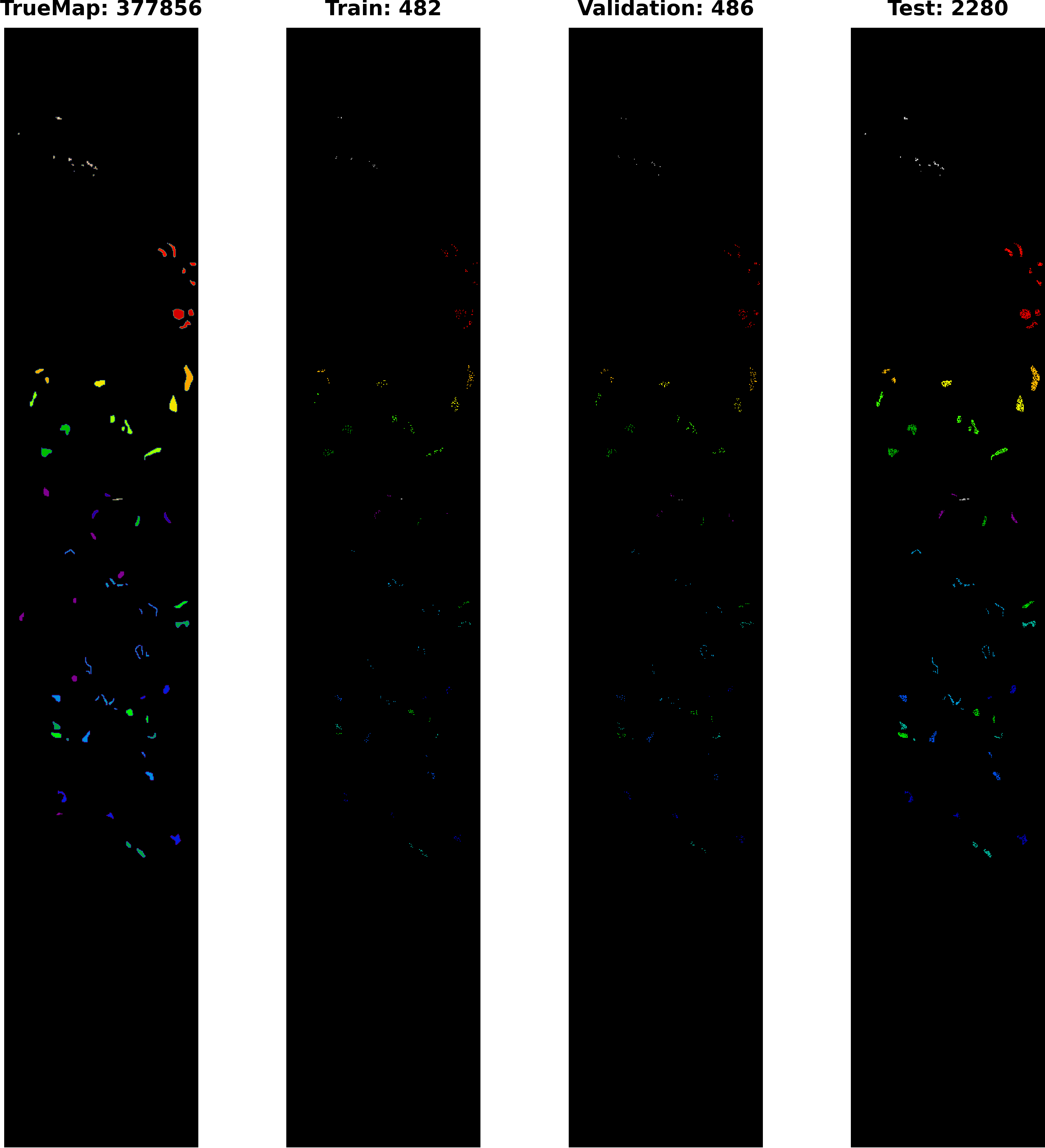
Botswana: The NASA EO-1 satellite acquired hyperspectral imagery of the Okavango Delta region in Botswana from 2001-2004 using the Hyperion sensor to collect 30m resolution data across 242 bands from 400-2500nm over a 7.7km strip. The data analyzed from May 31, 2001, consisted of observations of 14 land cover classes representing seasonal swamps, occasional swamps, and drier woodlands in the distal delta region after preprocessing removed uncalibrated and noisy bands covering water absorption and retaining 145 bands. The disjoint train, validation, and test samples are presented in Table V and Figure 6.

TABLE V: Botswana Dataset: Disjoint sets of training (Tr), validation (Va), and test (Te) samples were chosen, with their geographical locations (Excluding background samples) illustrated in Figure 6, to train various SOTA models.

Class	Tr	Va	Te	Class	Tr	Va	Te
Water	40	41	189	Island Interior	30	30	143
Hippo Grass	15	15	71	Woodlands	47	47	220
Floodplain Grasses 1	37	38	176	Acacia Shrublands	37	37	174
Floodplain Grasses 2	32	32	151	Acacia Grasslands	45	46	214
Reeds 1	40	40	189	Short Mopane	27	27	127
Riparian	40	40	189	Mixed Mopane	40	40	188
Firescar 2	38	39	182	Exposed Soils	14	14	67

Figure 6: Botswana Dataset: Geographical locations of the disjoint train, validation, and test samples presented in Table V.

III-B Experimental Settings

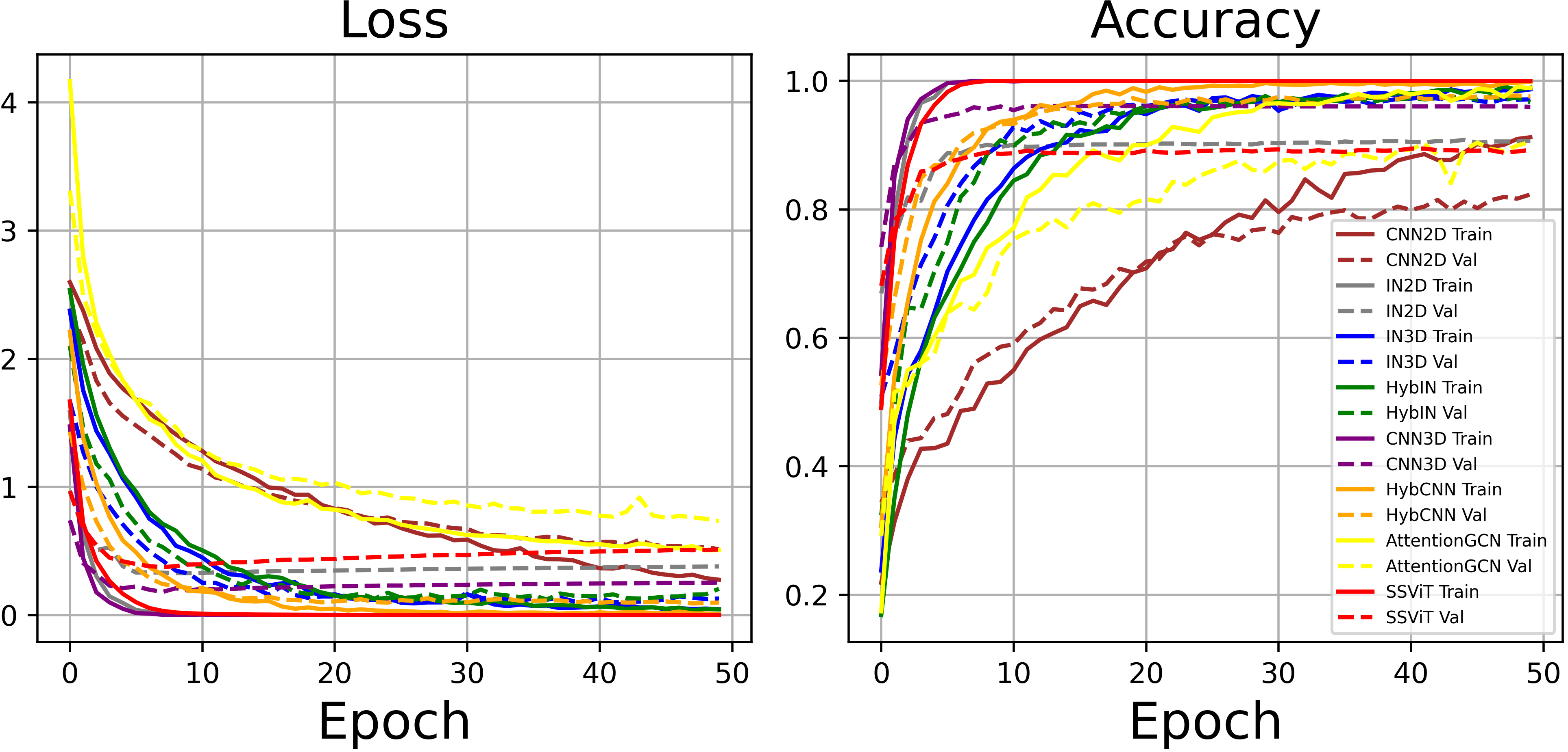
In this section, we present comprehensive experimental settings for various deep learning models, including 3D CNN [19], Hybrid Inception Net [37], 3D Inception Net [38], 2D Inception Net [39], 2D CNN [40], Hybrid CNN [41], Attention Graph CNN [21], and Spatial-Spectral Transformer [23]. Prior to training, 3D overlapped patches are extracted using an $8\times 8$ window size, as outlined in Algorithm 1. All models in this study are trained using the Adam optimizer with a learning rate of 0.0001, a decay rate of 1e-06, and a batch size of 56 for 50 epochs. The loss and accuracy trend is presented in Figure 7 for all the competing methods.

Figure 7: Loss and Accuracy trends for all the competing methods.

The 2D CNN model is trained using four convolutional layers with kernel sizes of $(3\times 3\times 8,16,32,64)$ and the same padding with $(8,16,32,64)$ number of filters, respectively. Following the convolutional layers, two dense layers are utilized with a dropout rate of 0.4%. Finally, a classification layer is added with the number of output units corresponding to the number of classes in the HSI dataset. The 3D CNN model is trained using four convolutional layers with kernel sizes of $(3\times 3\times 7,5,3,3)$ with $(8,16,32,64)$ number of filters, respectively. Following the convolutional layers, two dense layers are utilized and finally, a classification layer is added with the number of output units corresponding to the number of classes in the HSI dataset. The Hybrid CNN model is trained using three 3D convolutional layers with kernel sizes of $(3\times 3\times 7,5,3)$, followed by a reshaped layer to transform the features into 2D to learn spatial features using $3\times 3)$ kernel with 64 filters. Following the convolutional layers, two dense layers are utilized with a dropout rate of 0.4%. Finally, a classification layer is added with the number of output units corresponding to the number of classes in the HSI dataset.

The 2D Inception Net architecture consists of three blocks with the following configurations. In the first block, three 2D convolutional layers are used. The first layer employs a $(1\times 1)$ kernel with 30 filters, the second layer uses a $(3\times 3)$ kernel with 20 filters, and the third layer utilizes a $(1\times 1)$ kernel with 10 filters. In the second block, three 2D convolutional layers are utilized. The first layer has a $(1\times 1)$ kernel with 40 filters, the second layer employs a $(5\times 5)$ kernel with 20 filters, and the third layer uses a $(1\times 1)$ kernel with 10 filters. The third block begins with a 2D max pooling operation using a $(3\times 3)$ kernel and the same padding. This is followed by two 2D convolutional layers with $(1\times 1)$ kernels and the same padding. The filters for these layers are set to 20 and 10, respectively. Afterward, the outputs from all three blocks are concatenated, and a convolutional layer with a $(1\times 1)$ kernel and 128 filters is applied. Following the convolutional layer, two dense layers are deployed. Finally, a classification layer is added with the number of output units corresponding to the number of classes in the HSI dataset.

The 3D Inception Net architecture consists of three blocks with the following configurations. In the first block, three 3D convolutional layers are used. The first layer employs a $(5\times 5\times 7)$ kernel with 30 filters, the second layer uses a $(3\times 3\times 5)$ kernel with 20 filters, and the third layer utilizes a $(3\times 3\times 3)$ kernel with 10 filters and the same padding in all three layers. In the second block, three 3D convolutional layers are utilized. The first layer has a $(5\times 5\times 7)$ kernel with 40 filters, the second layer employs a $(3\times 3\times 5)$ kernel with 20 filters, and the third layer uses a $(3\times 3\times 3)$ kernel with 10 filters and the same padding in all three layers. The third block begins with three 3D convolutional layers with $(5\times 5\times 7)$ kernel with 60 filters, the second layer uses a $(3\times 3\times 5)$ kernel with 30 filters, and the third layer utilizes a $(3\times 3\times 3)$ kernel with 10 filters and the same padding in all three layers. Afterward, the outputs from all three blocks are concatenated, and a convolutional layer with a $(1\times 1\times 1)$ kernel and 128 filters is applied. Following the convolutional layer, two dense layers are deployed with a 0.4% dropout rate. Finally, a classification layer is added with the number of output units corresponding to the number of classes in the HSI dataset.

(a) 2D CNN

(b) 3D CNN

(c) Hybrid CNN

(d) 2D IN

(e) 3D IN

(f) Hybrid IN

(g) GCN

(h) Transformer

Figure 8: Indian Pines Dataset: Land cover maps for disjoint validation, test, and the entire HSI used as a test set are provided. Comprehensive class-wise results can be found in Table VI.

TABLE VI: Indian Pines Dataset: Per class comparative results of various SOTA models are showcased on disjoint validation and test sets. Additionally, results on the entire HSI dataset serving as the test set are also presented. The comparative methods include 3D CNN [19], Hybrid Inception Net (Hybrid IN) [37], 3D Inception Net (3D IN) [38], 2D Inception Net (2D IN) [39], 2D CNN [40], Hybrid CNN [41], Attention Graph CNN (Attention GCN) [21], and Spatial-Spectral Transformer [23]. The geographical maps for each model for disjoint validation, test, and complete test are presented in Figure 8.

Class	2D CNN			3D CNN			Hybrid CNN			2D IN			3D IN			Hybrid IN			Attention GCN			SSViT
	Va	Te	HSI	Va	Te	HSI	Va	Te	HSI	Va	Te	HSI	Va	Te	HSI	Va	Te	HSI	Va	Te	HSI	Va	Te	HSI
Alfalfa	57.14	69.69	99.87	85.71	75.75	99.92	100.00	96.97	99.99	100.00	93.94	99.98	100.00	90.91	99.97	100.00	93.94	99.98	71.43	60.61	99.86	100.00	90.91	99.97
Corn-notill	74.76	75.4	78.36	92.52	94.10	94.75	92.53	92.80	93.77	84.58	84.20	86.62	97.66	97.30	97.76	95.33	96.00	96.50	76.64	71.30	75.70	85.51	84.70	87.11
Corn-mintill	76.8	81.06	82.77	96.00	97.76	97.83	97.60	99.83	99.52	84.80	86.40	88.19	96.80	98.45	98.43	97.60	99.66	99.40	60.80	61.96	66.14	82.4	84.34	86.39
Corn	58.33	45.78	54.85	94.44	89.16	91.56	94.44	95.18	95.78	88.89	79.52	83.97	100.00	98.80	99.16	88.89	88.55	90.30	63.89	53.61	62.03	58.33	48.80	57.81
Grass-pasture	94.44	94.10	95.03	97.22	96.76	97.31	98.61	97.94	98.34	95.83	95.28	96.07	98.61	97.05	97.72	95.83	96.76	97.10	90.28	89.97	91.30	94.44	96.17	96.48
Grass-trees	100.	99.41	99.58	99.09	99.41	99.45	100.00	99.80	99.86	98.18	99.41	99.32	100.00	99.80	99.86	100.00	100.00	100.00	98.18	98.63	98.77	99.09	99.22	99.32
Grass-mowed	0.	0.	7.14	100.00	100.00	100.00	100.00	100.00	100.00	75.00	70.00	75.00	75.00	70.00	75.00	25.00	20.00	25.00	25.00	5.00	14.29	75.00	75.00	78.57
Hay-windrowed	98.611	98.50	98.74	100	99.70	99.79	100.00	100.00	100.00	100.00	98.21	98.74	100.00	100.00	100.00	100.00	100.00	100.00	98.61	95.52	96.65	98.61	99.40	99.37
Oats	0.	0.	5.0	66.66	71.43	75.00	66.67	85.71	85.00	33.33	71.43	70.00	0.00	28.57	35.00	0.00	28.57	30.00	0.00	21.43	30.00	0.00	78.57	70.00
Soybean-notill	75.34	74.44	77.77	92.47	91.34	92.80	91.78	93.10	93.93	86.30	81.64	85.08	91.78	94.42	94.86	88.36	91.48	92.18	81.51	79.00	82.41	82.19	82.97	85.39
Soybean-mintill	85.05	88.24	89.16	97.83	97.27	97.76	99.73	99.71	99.76	89.40	92.15	92.91	98.10	98.49	98.66	98.91	98.72	98.94	86.14	87.73	89.33	91.58	92.03	93.16
Soybean-clean	58.42	63.22	67.11	92.13	96.88	96.63	93.26	96.88	96.80	91.01	90.87	92.24	89.89	97.12	96.46	97.75	96.88	97.47	50.56	49.76	56.16	79.78	80.53	83.31
Wheat	83.87	95.13	94.14	100.00	100.00	100.00	100.00	100.00	100.00	96.77	99.31	99.02	100.00	97.92	98.54	100.00	98.61	99.02	96.77	92.36	94.15	93.55	99.31	98.54
Woods	97.36	97.40	97.78	96.32	97.29	97.55	98.95	99.32	99.37	98.42	99.10	99.13	98.95	98.53	98.81	98.95	99.21	99.30	97.37	97.18	97.63	97.89	96.73	97.39
Buildings	75.86	81.91	83.67	100	97.79	98.45	100.00	98.89	99.22	86.21	92.25	92.49	100.00	98.15	98.70	100.00	97.42	98.19	77.58	75.65	79.53	93.10	94.83	95.34
Stone-Steel	50.	83.33	79.56	92,86	96.97	96.77	100.00	100.00	100.00	92.86	98.48	97.85	100.00	100.00	100.00	100.00	100.00	100.00	78.57	83.33	84.95	92.86	100.00	98.92
Kappa	79.85	81.91	90.23	95.41	95.75	97.78	96.74	97.36	98.58	89.35	89.88	94.74	96.74	97.38	98.59	96.22	96.68	98.22	79.67	78.29	88.76	87.86	88.29	93.93
OA	82.33	84.17	93.10	95.97	96.27	98.43	97.14	97.69	99.00	90.64	91.13	96.29	97.14	97.70	99.00	96.69	97.09	98.74	82.20	81.06	92.08	89.34	89.74	95.71
AA	67.88	71.73	75.66	93.95	93.85	95.97	95.85	97.26	97.58	87.60	89.51	91.04	90.42	91.59	93.06	87.86	87.86	88.96	72.08	70.19	76.18	87.72	87.72	89.19
Time (S)	1.54	1.68	8.74	0.45	1.39	9.80	0.53	0.81	8.64	0.85	1.39	10.96	1.48	3.14	14.84	0.89	2.68	12.75	1.18	1.38	10.27	1.28	2.24	14.72

(a) 2D CNN

(b) 3D CNN

(c) Hybrid CNN

(d) 2D IN

(e) 3D IN

(f) Hybrid IN

(g) GCN

(h) Transformer

Figure 9: Pavia University Dataset: Land cover maps for disjoint validation, test, and the entire HSI used as a test set are provided. Comprehensive class-wise results can be found in Table VII.

TABLE VII: Pavia University Dataset: Per class comparative results of various SOTA models are showcased on disjoint validation and test sets. Additionally, results on the entire HSI dataset serving as the test set are also presented. The comparative methods include 3D CNN [19], Hybrid Inception Net (Hybrid IN) [37], 3D Inception Net (3D IN) [38], 2D Inception Net (2D IN) [39], 2D CNN [40], Hybrid CNN [41], Attention Graph CNN (Attention GCN) [21], and Spatial-Spectral Transformer [23]. The geographical maps for each model for disjoint validation, test, and complete test are presented in Figure 9.

Class	2D CNN			3D CNN			Hybrid CNN			2D IN			3D IN			Hybrid IN			Attention GCN			SSViT
	Va	Te	HSI	Va	Te	HSI	Va	Te	HSI	Va	Te	HSI	Va	Te	HSI	Va	Te	HSI	Va	Te	HSI	Va	Te	HSI
Asphalt	99.70	99.87	99.99	99.80	99.78	99.99	100.00	99.83	99.99	98.59	98.97	99.96	99.40	99.05	99.97	100.00	100.00	100.00	98.29	98.32	99.94	98.29	98.15	99.94
Meadows	99.96	99.95	99.96	99.96	100.00	99.99	99.96	99.99	99.99	99.89	99.96	99.96	99.96	100.00	99.99	99.89	99.91	99.92	99.82	99.90	99.89	100.00	98.91	99.94
Gravel	94.29	94.35	95.19	98.41	97.55	98.04	98.41	98.50	98.71	93.65	93.67	94.62	97.46	97.76	98.05	97.14	97.69	97.95	87.30	85.17	86.04	89.21	88.76	90.52
Trees	98.91	99.07	99.18	99.13	99.39	99.25	99.13	99.49	99.51	96.96	97.86	98.04	98.26	98.97	99.02	99.78	99.86	99.87	95.43	96.41	96.57	97.39	98.60	98.63
Painted	100.00	100.00	100.00	100.00	100.00	100.00	100.00	100.00	100.00	100.00	99.89	99.93	100.00	100.00	100.00	100.00	100.00	100.00	100.00	100.00	100.00	100.00	100.00	100.00
Soil	99.87	99.20	99.42	100.00	100.00	100.00	100.00	100.00	100.00	99.34	98.64	98.95	100.00	99.94	99.96	100.00	100.00	100.00	100.00	99.43	99.60	99.73	99.03	99.28
Bitumen	98.00	98.82	98.87	99.50	99.36	99.47	99.50	99.79	99.77	96.50	97.96	98.05	99.50	99.79	99.77	100.00	99.68	99.77	94.00	93.34	94.29	97.00	96.24	96.92
Bricks	96.56	97.05	97.42	98.73	99.19	99.24	99.46	99.34	99.46	96.56	96.47	97.01	99.28	99.50	99.54	99.28	98.80	99.02	96.56	97.40	97.64	94.38	93.91	94.89
Shadows	100.00	98.79	99.16	99.30	99.40	99.47	99.30	99.85	99.79	100.00	98.49	98.94	100.00	99.85	99.94	100.00	99.70	99.79	99.30	99.25	99.37	99.30	99.55	99.58
Kappa	98.95	98.95	99.55	99.57	99.60	99.83	99.69	99.73	99.88	98.31	98.40	99.31	99.42	99.48	99.77	99.65	99.62	99.84	97.62	97.61	98.90	97.81	97.69	99.02
OA	99.21	99.21	99.86	99.67	99.70	99.95	99.77	99.79	99.96	98.72	98.79	99.79	99.56	99.61	99.93	99.74	99.72	99.95	98.21	98.20	99.66	98.39	98.26	99.70
AA	98.59	98.57	98.80	99.43	99.41	99.52	99.53	99.64	99.69	97.94	97.99	98.38	99.32	99.43	99.58	99.57	99.51	99.59	96.74	96.58	97.04	97.26	97.13	97.74
Time (S)	1.05	2.91	85.48	1.42	3.52	90.00	0.80	5.47	83.94	1.47	3.81	85.17	2.98	11.53	139.04	2.90	7.13	105.40	1.80	5.01	100.10	2.49	10.61	144.50

(a) 2D CNN

(b) 3D CNN

(c) Hybrid CNN

(d) 2D IN

(e) 3D IN

(f) Hybrid IN

(g) GCN

(h) Transformer

Figure 10: University Houston Dataset: Land cover maps for disjoint validation, test, and the entire HSI used as a test set are provided. Comprehensive class-wise results can be found in Table VIII.

TABLE VIII: University of Houston Dataset: Per class comparative results of various SOTA models are showcased on disjoint validation and test sets. Additionally, results on the entire HSI dataset serving as the test set are also presented. The comparative methods include 3D CNN [19], Hybrid Inception Net (Hybrid IN) [37], 3D Inception Net (3D IN) [38], 2D Inception Net (2D IN) [39], 2D CNN [40], Hybrid CNN [41], Attention Graph CNN (Attention GCN) [21], and Spatial-Spectral Transformer [23]. The geographical maps for each model for disjoint validation, test, and complete test are presented in Figure 10.

Class	2D CNN			3D CNN			Hybrid CNN			2D IN			3D IN			Hybrid IN			Attention GCN			SSViT
	Va	Te	HSI	Va	Te	HSI	Va	Te	HSI	Va	Te	HSI	Va	Te	HSI	Va	Te	HSI	Va	Te	HSI	Va	Te	HSI
Healthy grass	97.33	96.69	99.99	97.00	97.95	99.99	99.33	99.09	99.99	98.67	98.63	99.99	99.33	98.86	99.99	100.00	99.54	99.99	94.33	94.18	99.99	98.00	98.17	99.99
Stressed grass	99.67	99.20	99.36	99.67	98.86	99.12	99.67	98.97	99.20	99.67	98.97	99.20	99.67	99.32	99.44	99.34	98.41	98.72	98.67	98.41	98.56	99.34	98.75	98.96
Synthetic grass	98.81	99.39	99.28	95.83	96.31	96.41	97.02	97.95	97.85	95.24	92.83	93.83	98.21	98.16	98.28	98.81	98.57	98.71	97.62	97.54	97.70	97.02	96.11	96.56
Trees	100.00	99.77	99.84	98.33	98.85	98.79	98.99	99.54	99.44	99.33	98.74	98.95	99.67	99.89	99.84	99.33	99.66	99.60	90.30	89.44	90.03	97.32	97.93	97.91
Soil	100.00	100.00	100.00	99.66	100.00	99.92	100.00	100.00	100.00	100.00	99.89	99.92	100.00	100.00	100.00	100.00	100.00	100.00	99.66	99.77	99.76	100.00	99.89	99.92
Water	78.21	82.46	82.46	92.31	95.18	94.77	97.44	99.12	98.77	79.49	85.09	84.62	92.31	91.23	92.00	97.44	97.81	97.85	75.64	75.44	76.92	94.87	95.61	95.69
Residential	95.07	94.14	94.72	96.05	96.28	96.45	98.36	98.54	98.58	95.39	94.26	94.87	98.36	97.75	98.03	98.68	98.09	98.34	84.54	86.26	86.67	92.76	94.37	94.32
Commercial	85.28	85.19	85.85	97.66	97.70	97.83	97.66	97.82	97.91	99.33	95.64	96.78	94.98	97.82	97.27	96.32	97.36	97.27	81.94	84.27	84.65	93.98	96.90	96.38
Road	91.67	89.28	90.50	94.33	92.82	93.61	97.33	95.78	96.41	94.33	91.33	92.57	94.00	92.93	93.61	94.33	92.93	93.69	83.00	80.62	82.35	91.66	91.33	91.93
Highway	93.90	93.83	94.21	98.98	98.72	98.86	95.93	95.81	95.93	97.63	96.97	97.31	99.32	99.30	99.35	99.32	99.30	99.35	91.53	93.95	93.72	97.63	97.21	97.47
Railway	95.27	96.30	96.28	98.31	98.15	98.30	100.00	99.77	99.84	99.66	99.65	99.68	99.32	99.31	99.35	99.66	98.03	98.54	93.24	91.56	92.47	98.99	98.38	98.62
Parking Lot 1	94.93	95.49	95.62	98.99	99.88	99.68	98.65	99.54	99.35	97.64	98.03	98.05	98.99	99.77	99.59	98.99	99..88	99.68	95.27	93.52	94.32	98.65	99.19	99.10
Parking Lot 2	63.39	62.92	65.25	79.46	81.46	82.09	93.75	96.96	96.38	85.71	88.15	88.27	94.64	94.83	95.10	96.43	96.05	96.38	50.00	52.88	55.01	59.82	68.99	68.65
Tennis Court	97.09	96.67	96.96	99.03	98.00	98.36	99.03	98.67	98.83	90.29	87.00	88.55	99.03	100.00	99.77	96.12	100.00	99.07	90.29	90.00	90.65	97.09	95.67	96.26
Running Track	100.00	99.78	99.85	100.00	100.00	100.00	100.00	100.00	100.00	100.00	98.92	99.24	100.00	100.00	100.00	100.00	100.00	100.00	95.27	92.42	94.09	100.00	100.00	100.00
Kappa	93.91	93.7	96.99	97.00	97.14	98.61	98.29	98.38	99.20	96.85	95.93	98.16	98.05	98.17	99.11	98.38	98.23	99.17	89.35	89.13	94.79	95.44	96.01	98.02
OA	94.37	94.18	99.88	97.23	97.36	99.94	98.42	98.50	99.97	97.09	96.24	99.92	98.20	98.31	99.96	98.50	98.37	99.97	90.16	89.96	99.79	95.79	96.31	99.92
AA	92.71	92.74	93.34	96.37	96.68	96.95	98.21	98.50	98.56	95.49	94.94	95.46	97.86	97.94	98.11	98.32	98.37	99.48	88.23	88.02	89.13	94.48	95.23	95.45
Time (S)	1.63	2.54	320.98	0.76	1.58	323.42	0.47	1.12	309.30	0.63	1.38	362.58	1.78	4.55	542.21	1.24	2.85	449.60	2.07	2.73	342.90	2.04	3.76	533.75

TABLE IX: Botswana Dataset: Per class comparative results of various SOTA models are showcased on disjoint validation and test sets. Additionally, results on the entire HSI dataset serving as the test set are also presented. The comparative methods include 3D CNN [19], Hybrid Inception Net (Hybrid IN) [37], 3D Inception Net (3D IN) [38], 2D Inception Net (2D IN) [39], 2D CNN [42], Hybrid CNN [41], Attention Graph CNN (Attention GCN) [21], and Spatial-Spectral Transformer [23]. The geographical maps for each model for disjoint validation, test, and complete test are presented in Figure 11.

Class	2D CNN			3D CNN			Hybrid CNN			2D IN			3D IN			Hybrid IN			Attention GCN			SSViT
	Va	Te	HSI	Va	Te	HSI	Va	Te	HSI	Va	Te	HSI	Va	Te	HSI	Va	Te	HSI	Va	Te	HSI	Va	Te	HSI
Water	100.00	100.00	100.00	100.00	98.94	99.99	97.56	100.00	99.99	100.00	100.00	100.00	100.00	100.00	100.00	100.00	100.00	100.00	97.56	99.47	99.99	100.00	100.00	100.00
Hippo Grass	53.33	53.52	60.40	100.00	100.00	100.00	100.00	100.00	100.00	100.00	100.00	100.00	100.00	100.00	100.00	100.00	100.00	100.00	80.00	50.70	62.38	100.00	100.00	100.00
Floodplain Grasses 1	100.00	100.00	100.00	100.00	100.00	100.00	100.00	100.00	100.00	100.00	100.00	100.00	100.00	100.00	100.00	100.00	100.00	100.00	89.47	87.50	89.64	100.00	100.00	100.00
Floodplain Grasses 2	96.88	99.34	99.07	100.00	100.00	100.00	100.00	100.00	100.00	100.00	100.00	100.00	100.00	100.00	100.00	100.00	100.00	100.00	93.75	99.34	98.60	100.00	100.00	100.00
Reeds 1	87.5	92.06	92.19	100.00	99.47	99.63	95.00	97.35	97.40	87.5	90.48	91.45	90.00	94.18	94.42	97.50	100.00	99.63	92.50	95.24	95.54	87.50	93.12	93.31
Riparian	82.50	82.54	85.13	95.00	94.71	95.54	87.50	92.06	92.57	90.00	95.24	95.17	95.00	95.24	95.91	90.00	94.71	94.80	87.50	86.77	88.85	92.50	94.71	95.17
Firescar 2	100.00	98.35	98.84	100.00	98.90	99.23	100.00	100.00	100.00	100.00	100.00	100.00	100.00	100.00	100.00	100.00	100.00	100.00	100.00	100.00	100.00	100.00	100.00	100.00
Island Interior	96.67	98.60	98.52	100.00	95.10	96.55	100.00	96.50	97.54	100.00	95.80	97.04	100.00	100.00	100.00	100.00	100.00	100.00	86.67	93.01	93.10	100.00	100.00	100.00
Woodlands	82.98	85.00	86.94	97.87	96.36	97.13	100.00	100.00	100.00	100.00	95.45	96.82	100.00	100.00	100.00	100.00	100.00	100.00	100.00	98.64	99.04	100.00	97.73	98.41
Acacia Shrublands	100.00	100.00	100.00	100.00	100.00	100.00	100.00	100.00	100.00	100.00	100.00	100.00	100.00	100.00	100.00	100.00	100.00	100.00	97.30	88.51	91.53	100.00	100.00	100.00
Acacia Grasslands	93.48	97.66	97.38	100.00	100.00	100.00	100.00	100.00	100.00	93.48	95.79	96.07	97.83	99.07	99.02	100.00	100.00	100.00	93.48	85.51	88.85	97.83	99.07	99.02
Short Mopane	88.89	87.40	89.50	100.00	100.00	100.00	100.00	100.00	100.00	92.59	97.64	97.24	100.00	100.00	100.00	100.00	100.00	100.00	85.19	90.55	99.16	100.00	99.21	99.44
Mixed Mopane	100.00	100.00	100.00	100.00	100.00	100.00	100.00	100.00	100.00	100.00	99.47	99.63	100.00	100.00	100.00	100.00	100.00	100.00	95.00	94.15	95.15	100.00	99.47	99.62
Exposed Soils	92.86	89.55	91.58	92.86	97.01	96.84	100.00	100.00	100.00	92.85	92.54	93.68	92.86	95.52	95.79	92.86	97.01	96.84	71.43	70.15	74.74	92.86	97.01	96.84
Kappa	91.97	92.96	96.88	99.11	98.48	99.39	98.22	98.81	99.44	96.66	97.10	98.72	98.22	98.81	99.44	98.66	99.43	99.7	91.97	90.48	96.02	97.77	98.38	99.26
OA	92.59	93.51	99.95	99.18	98.60	99.99	98.35	98.90	99.99	96.91	97.32	99.98	98.35	98.90	99.99	98.77	99.47	99.99	92.59	91.23	99.94	97.94	98.51	99.98
AA	91.08	91.72	92.83	98.98	98.61	98.92	98.58	98.99	99.11	96.89	97.32	97.65	98.26	98.86	98.94	98.60	99.41	99.38	90.70	88.54	90.61	97.91	98.59	98.70
Time (S)	1.67	0.71	91.08	0.50	0.73	173.25	0.20	0.33	169.01	0.81	0.52	153.69	0.78	1.34	269.21	0.61	1.34	231.29	0.71	0.70	185.74	1.01	1.35	276.85

(a) 2D CNN

(b) 3D CNN

(c) Hybrid CNN

(d) 2D IN

(e) 3D IN

(f) Hybrid IN

(g) GCN

(h) Transformer

Figure 11: Botswana Dataset:

TABLE X: Salinas Dataset: Per class comparative results of various SOTA models are showcased on disjoint validation and test sets. Additionally, results on the entire HSI dataset serving as the test set are also presented. The comparative methods include 3D CNN [19], Hybrid Inception Net (Hybrid IN) [37], 3D Inception Net (3D IN) [38], 2D Inception Net (2D IN) [39], 2D CNN [40], Hybrid CNN [41], Attention Graph CNN (Attention GCN) [21], and Spatial-Spectral Transformer [23]. The geographical maps for each model for disjoint validation, test, and complete test are presented in Figure 12.

Class	2D CNN			3D CNN			Hybrid CNN			2D IN			3D IN			Hybrid IN			Attention GCN			SSViT
	Va	Te	HSI	Va	Te	HSI	Va	Te	HSI	Va	Te	HSI	Va	Te	HSI	Va	Te	HSI	Va	Te	HSI	Va	Te	HSI
Weeds 1	100	100	100	100	100	100	100	100	100	100	100	100	100	100	100	100	100	100	100	100	100	100	100	100
Weeds 2	100	100	100	99.64	100	99.95	100	100	100	100	100	100	100	100	100	100	100	100	100	100	100	100	100	100
Fallow	100	100	100	99.32	99.64	99.65	100	100	100	99.66	99.78	99.80	100	100	100	100	100	100	98.65	99.71	99.60	99.32	99.71	99.70
Fallow rough plow	100	99.90	99.93	100	100	100	100	100	100	100	99.80	99.86	100	100	100	99.52	100	99.93	98.56	99.28	99.21	99.52	99.90	99.86
Fallow smooth	97.26	98.19	98.32	99.25	99.20	99.33	98.76	99.20	99.07	97.26	97.55	97.87	99.75	100	99.96	99.75	99.95	99.93	98.01	97.87	98.21	98.76	98.51	98.77
Stubble	100	100	100	100	100	100	100	100	100	100	100	100	100	100	100	100	100	100	100	100	100	100	100	100
Celery	100	100	100	100	100	100	100	100	100	99.81	99.80	99.83	100	100	100	100	100	100	100	100	100	100	100	100
Grapes untrained	99.53	99.21	99.38	99.59	99.54	99.62	99.88	99.68	99.76	98.11	98.18	98.45	99.88	99.85	99.88	99.82	99.67	99.74	98.17	98.16	98.35	97.99	97.68	98.09
Soil vinyard develop	100	100	100	100	100	100	100	100	100	100	100	100	100	100	100	100	100	100	100	99.98	99.98	100	100	100
Corn Weeds	100	100	100	100	100	100	100	100	100	100	100	100	100	99.96	99.97	100	100	100	100	99.91	99.94	100	100	100
Lettuce 4wk	99.38	99.73	99.72	100	100	100	100	100	100	100	99.86	99.91	100	100	100	100	100	100	98.75	98.80	98.88	100	100	100
Lettuce 5wk	100	100	100	100	100	100	100	100	100	100	100	100	100	100	100	100	100	100	100	100	100	100	100	100
Lettuce 6wk	100	100	100	100	100	100	100	100	100	100	100	100	100	100	100	100	100	100	99.28	99.84	99.78	100	100	100
Lettuce 7wk	99.38	100	99.91	100	100	100	100	100	100	100	100	100	100	100	100	100	100	100	100	100	100	100	100	100
Vinyard untrained	97.25	96.91	97.37	99.82	99.84	99.86	99.91	99.86	99.89	95.41	95.48	96.15	99.72	99.88	99.88	100	99.72	99.81	95.60	94.99	95.46	97.80	96.76	97.40
Vinyard trellis	99.63	99.53	99.61	100	99.84	99.89	99.26	99.76	99.72	99.26	99.68	99.67	100	100	100	100	100	100	99.89	99.13	99.22	100	100	100
Kappa	99.29	99.23	99.59	99.78	99.81	99.89	99.86	99.85	99.92	98.67	98.72	99.31	99.92	99.94	99.97	99.93	99.88	99.94	98.63	98.60	99.20	99.09	98.88	99.42
OA	99.36	99.31	99.71	99.80	99.83	99.93	99.88	99.87	99.94	98.81	98.85	99.52	99.93	99.95	99.98	99.94	99.89	99.96	98.77	98.75	99.45	99.19	98.99	99.60
AA	99.53	99.59	99.64	99.85	99.88	99.89	99.86	99.91	99.90	99.35	99.38	99.47	99.96	99.98	99.98	99.94	99.96	99.96	99.12	99.23	99.29	99.59	99.53	99.61
Time (S)	1.23	5.56	44.41	1.45	5.56	47.61	0.82	5.56	47.67	2.84	5.67	43.78	5.33	14.52	72.51	2.85	9.15	61.40	3.07	5.93	49.99	2.87	20.92	78.67

(a) 2D CNN

(b) 3D CNN

(c) Hybrid CNN

(d) 2D IN

(e) 3D IN

(f) Hybrid IN

(g) GCN

(h) Transformer

Figure 12: Salinas Dataset: Land cover maps for disjoint validation, test, and the entire HSI used as a test set are provided. Comprehensive class-wise results can be found in Table X.

The hybrid Inception Net architecture consists of three blocks with the following configurations. In the first block, three 3D convolutional layers are used. The first layer has a $(5\times 5\times 7)$ kernel with 30 filters, the second layer uses a $(3\times 3\times 5)$ kernel with 20 filters, and the third layer employs a $(3\times 3\times 3)$ kernel with 10 filters. The same padding is applied in all three layers. Following the convolutional layer, a reshaped layer is used to convert the features from 3D to 2D. Next, a 2D max-pooling layer with a $(3\times 3)$ filter is applied, followed by three 2D convolutional layers. Each of these layers uses a $(1\times 1)$ kernel with 16, 32, and 64 filters, respectively. The same padding is used for all three layers. The same configuration is repeated for the second and third blocks, with the numbers of filters set to 40, 20, and 10 for the 3D convolutional layers, and 16, 32, and 64 for the 2D convolutional layers in the second block, and 60, 30, and 10 for the 3D convolutional layers, and 16, 32, and 64 for the 2D convolutional layers in the third block. Afterward, the outputs from all three blocks are concatenated, and a convolutional layer with a $(1\times 1\times 1)$ kernel and 128 filters is applied. Following the convolutional layer, two dense layers are deployed with a 0.4% dropout rate. Finally, a classification layer is added with the number of output units corresponding to the number of classes in the HSI dataset.

The Attention Graph-based CNN [21] and Transformers [23] models are trained according to the settings specified in their respective papers. The Transformer model, in particular, is used without the wavelet transformation and consists of 4 layers with 8 heads to compute the final maps. A dropout rate of 0.1 is applied to the classification layers. For more detailed information, please refer to the original papers.

III-C Experimental Results and Discussion

This section provides a detailed exploration of experimental results in comparison to the state-of-the-art (SOTA) works published in recent years. While many recent research endeavors present extensive experimental outcomes to highlight the strengths and weaknesses of their approaches, it is noteworthy that the experimental results in the literature may follow diverse protocols. For instance, the selection of training, validation, and test samples might be randomly done, and the percentage distribution may be identical. However, there could be variations in the geographical locations of each model, as these models may have undergone training, validation, and testing at different times. Comparative models may have been executed in multiple instances, either sequentially or in parallel, introducing a new set of training, validation, and test samples with the same number or percentage. Consequently, to ensure a fair comparison between the works proposed in the literature and the current study, it is imperative to employ identical experimental settings and execute them with the same set of training, validation, and test samples. This approach ensures a consistent and unbiased evaluation of the proposed methodologies against existing benchmarks.

A prevalent concern in the majority of recent literature is the presence of overlapping training and test samples. When training and validation samples are randomly selected, with or without considering the aforementioned point, the data split often includes overlapping samples. This situation introduces bias to the model, as overlapping implies the model has already encountered the training and validation samples, leading to inflated accuracy metrics. To prevent this issue, this study ensures that, despite the random selection of samples, the intersection between training, test, and validation samples remains consistently empty for all competing methods. This measure aims to maintain the integrity of the model evaluation process and uphold the reliability of accuracy assessments.

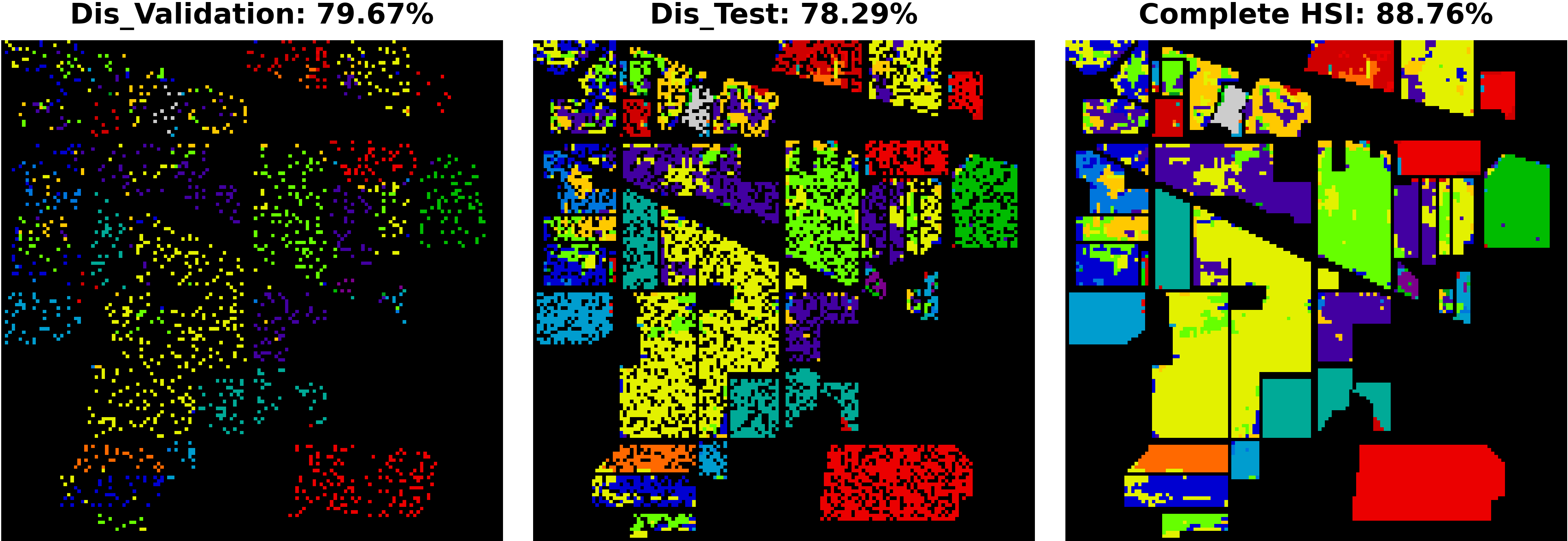
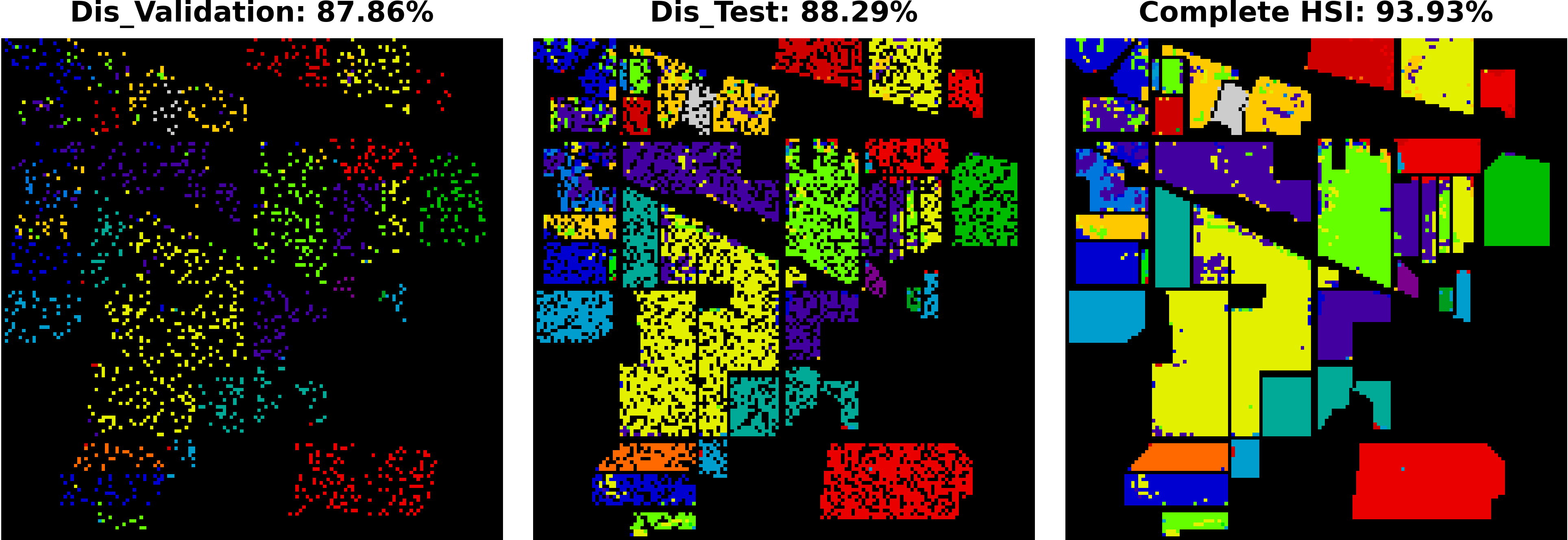
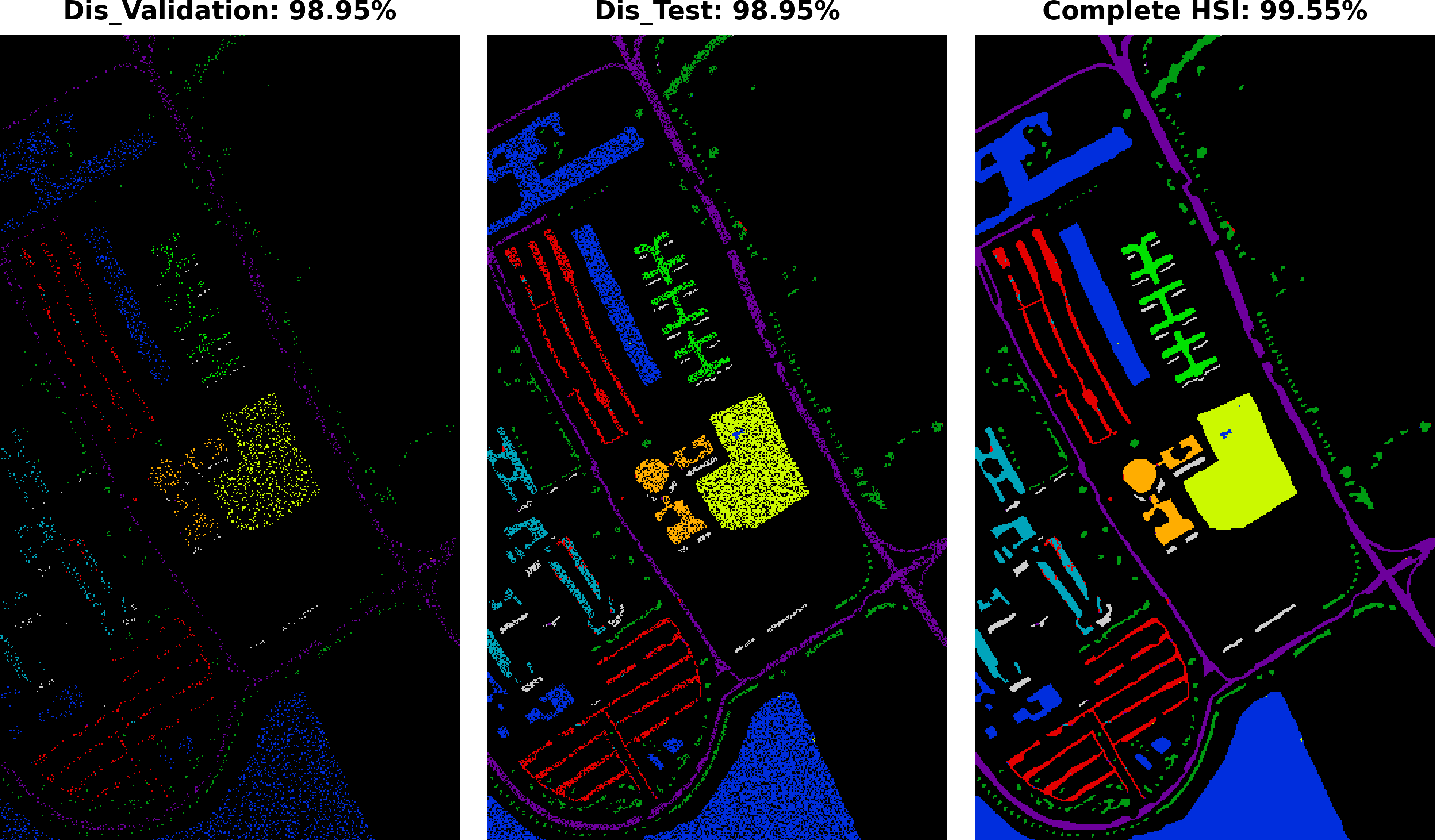
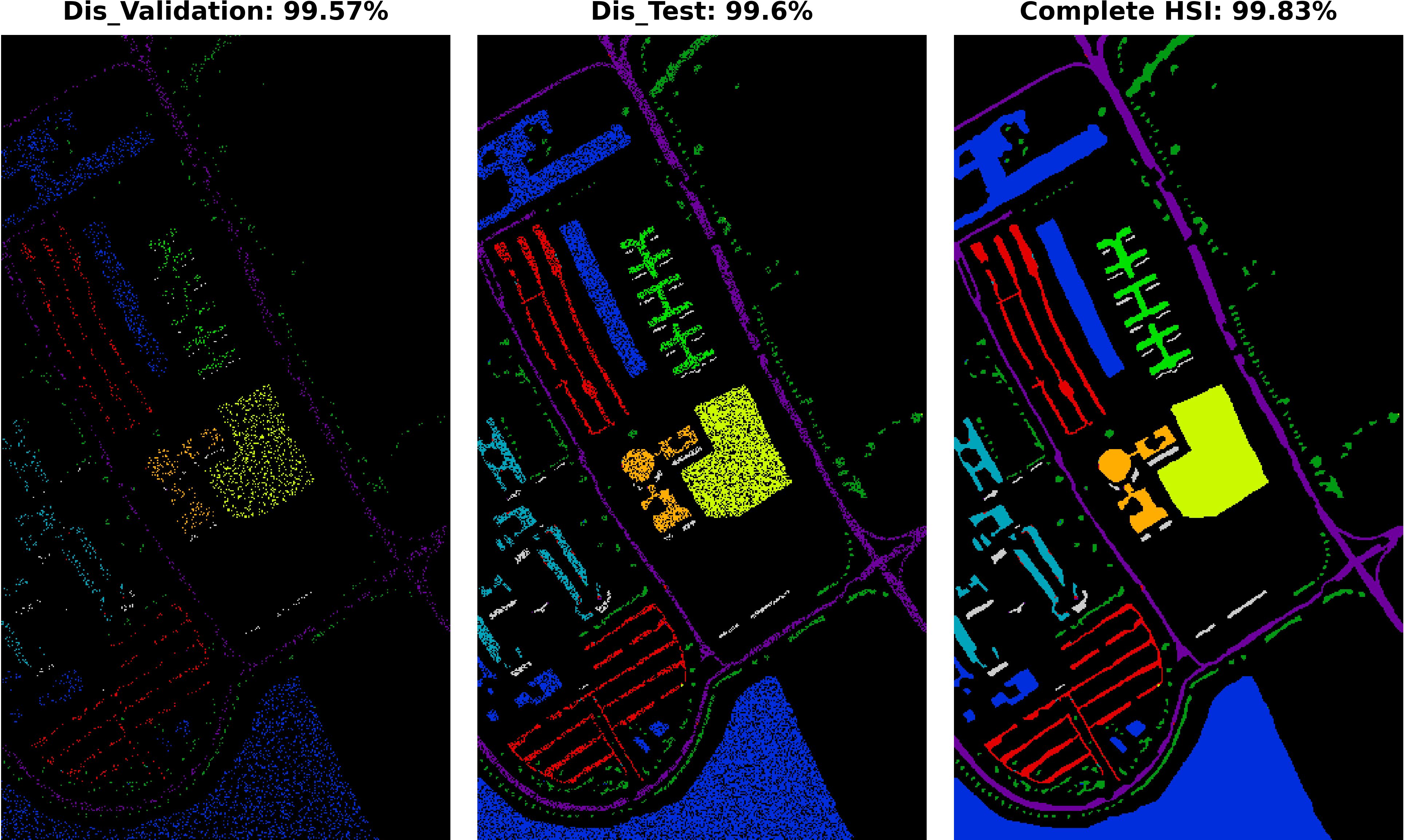
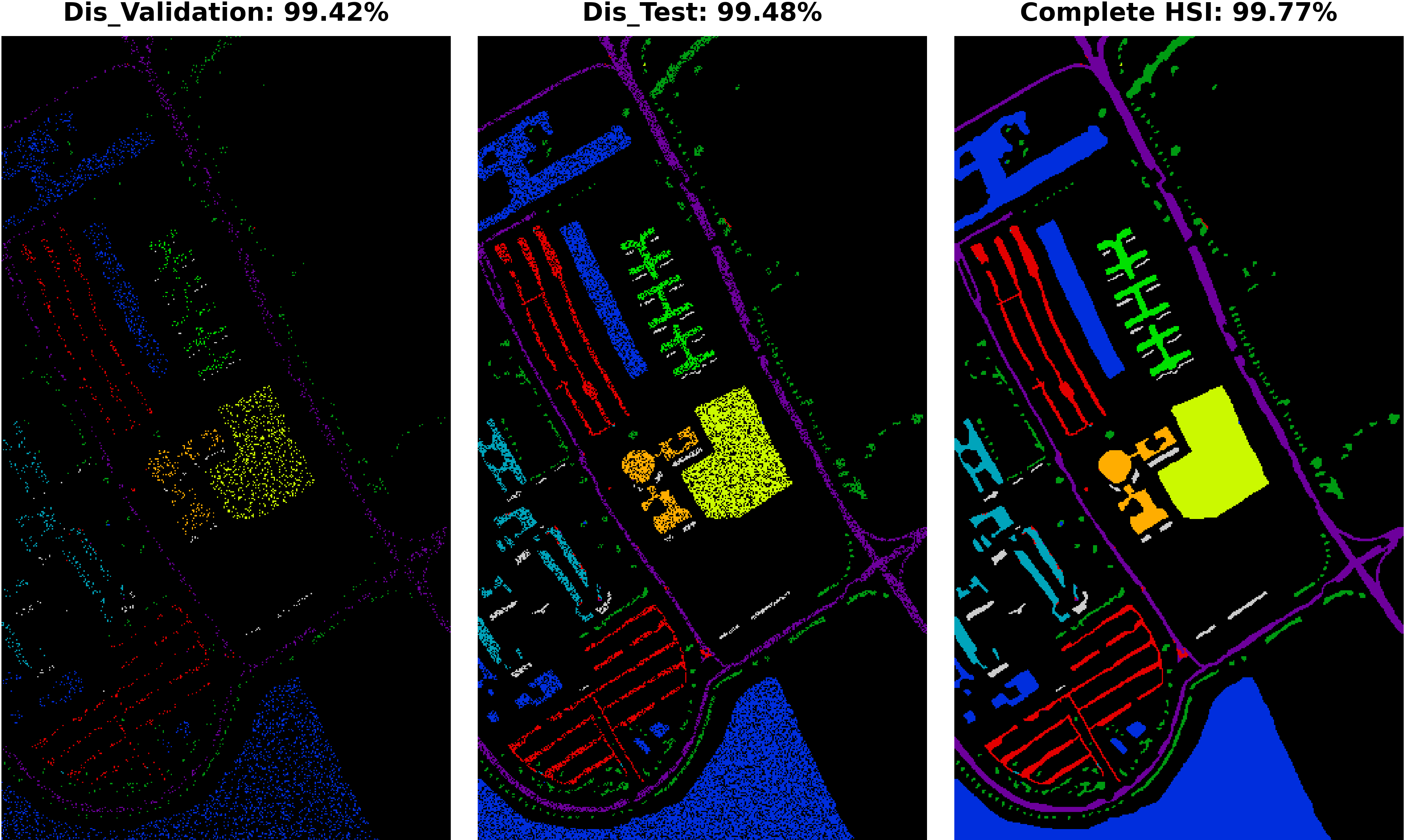
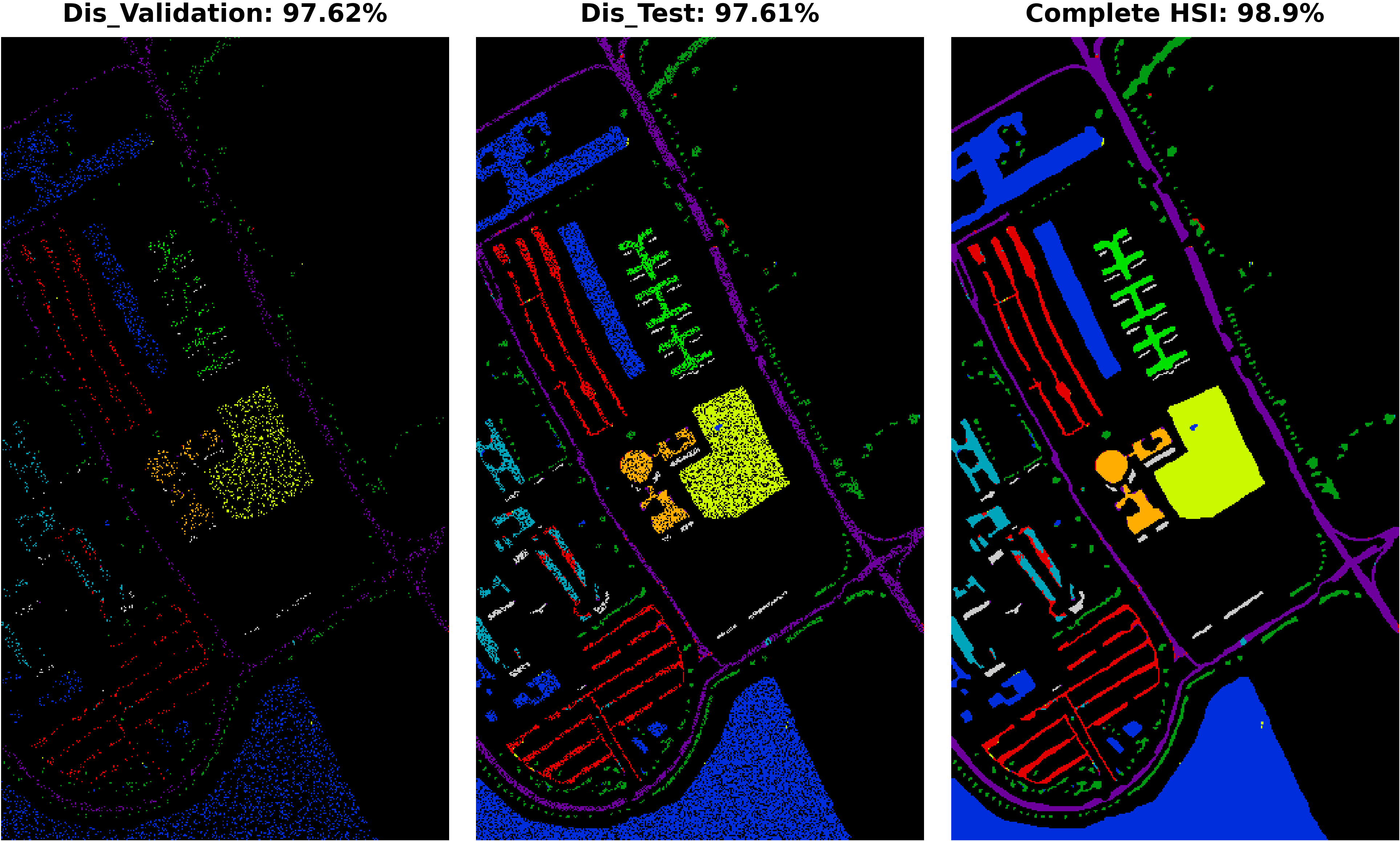
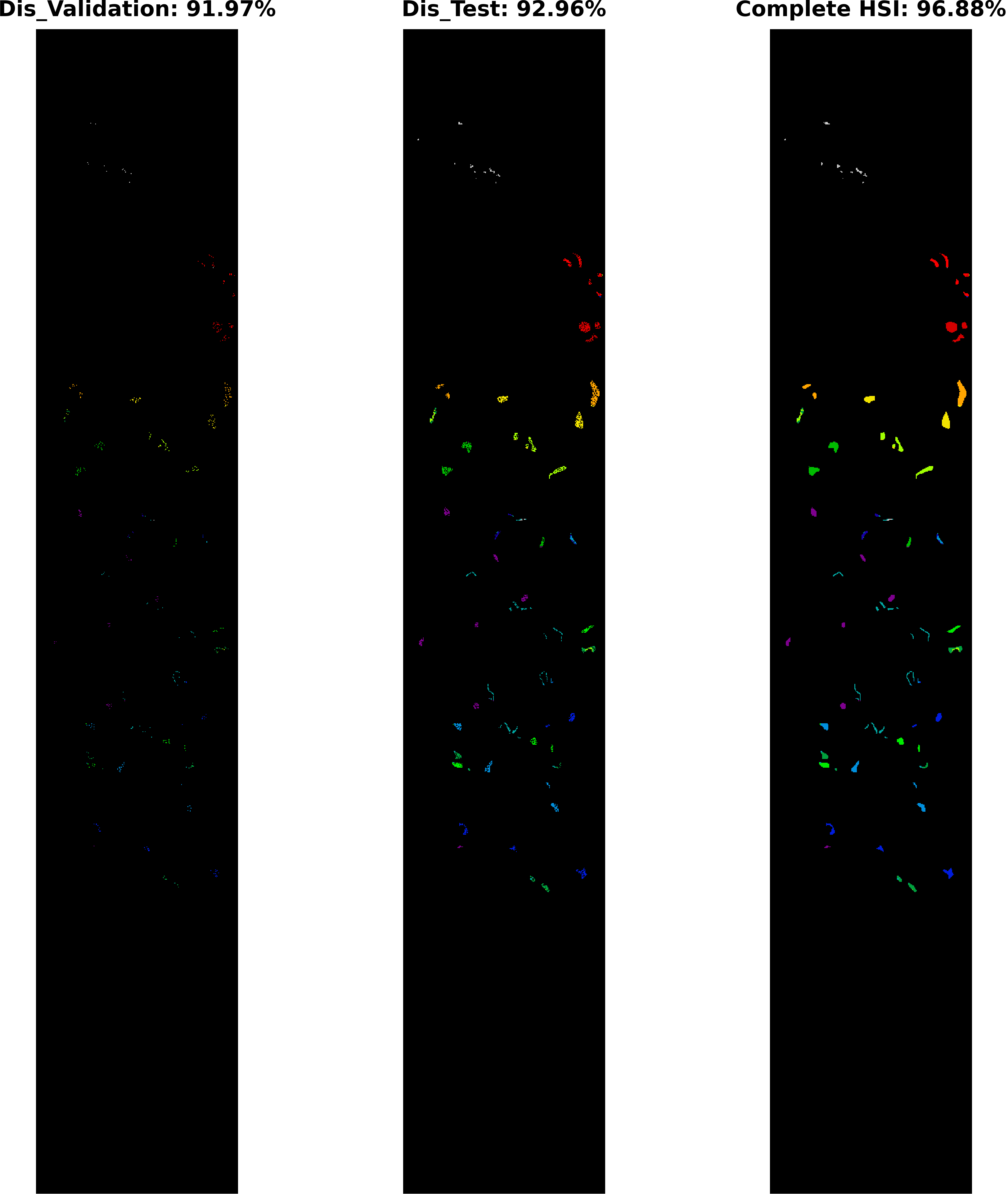
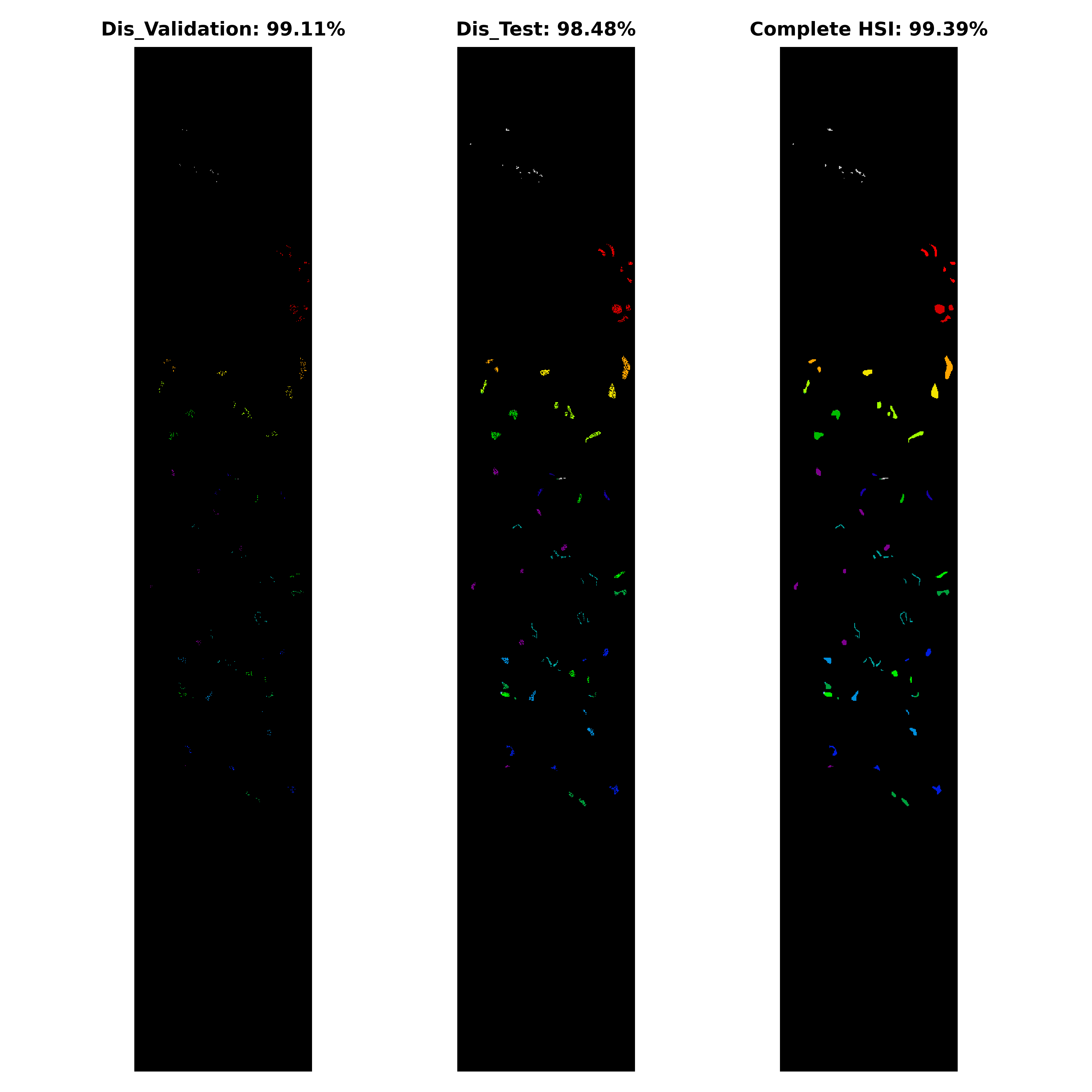
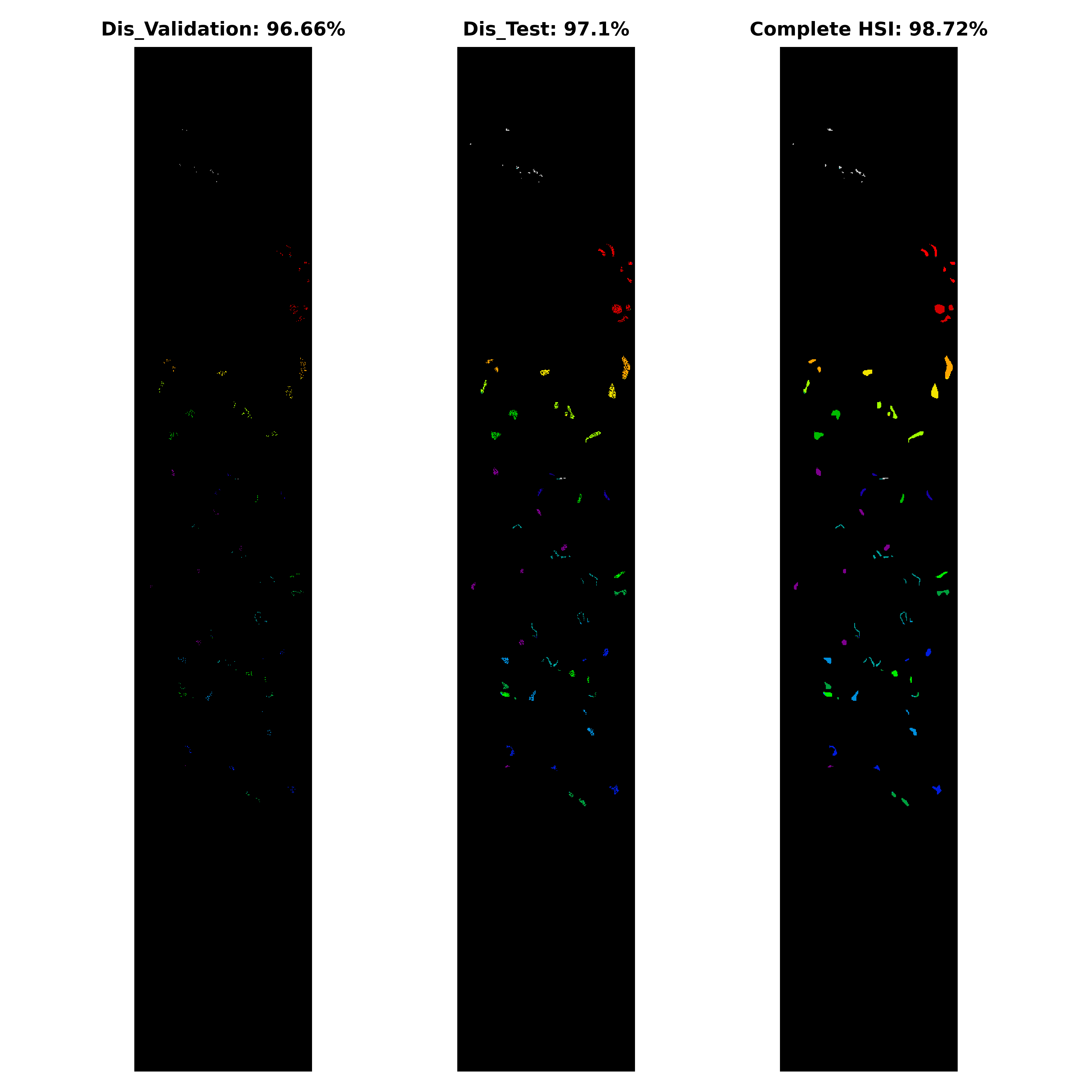
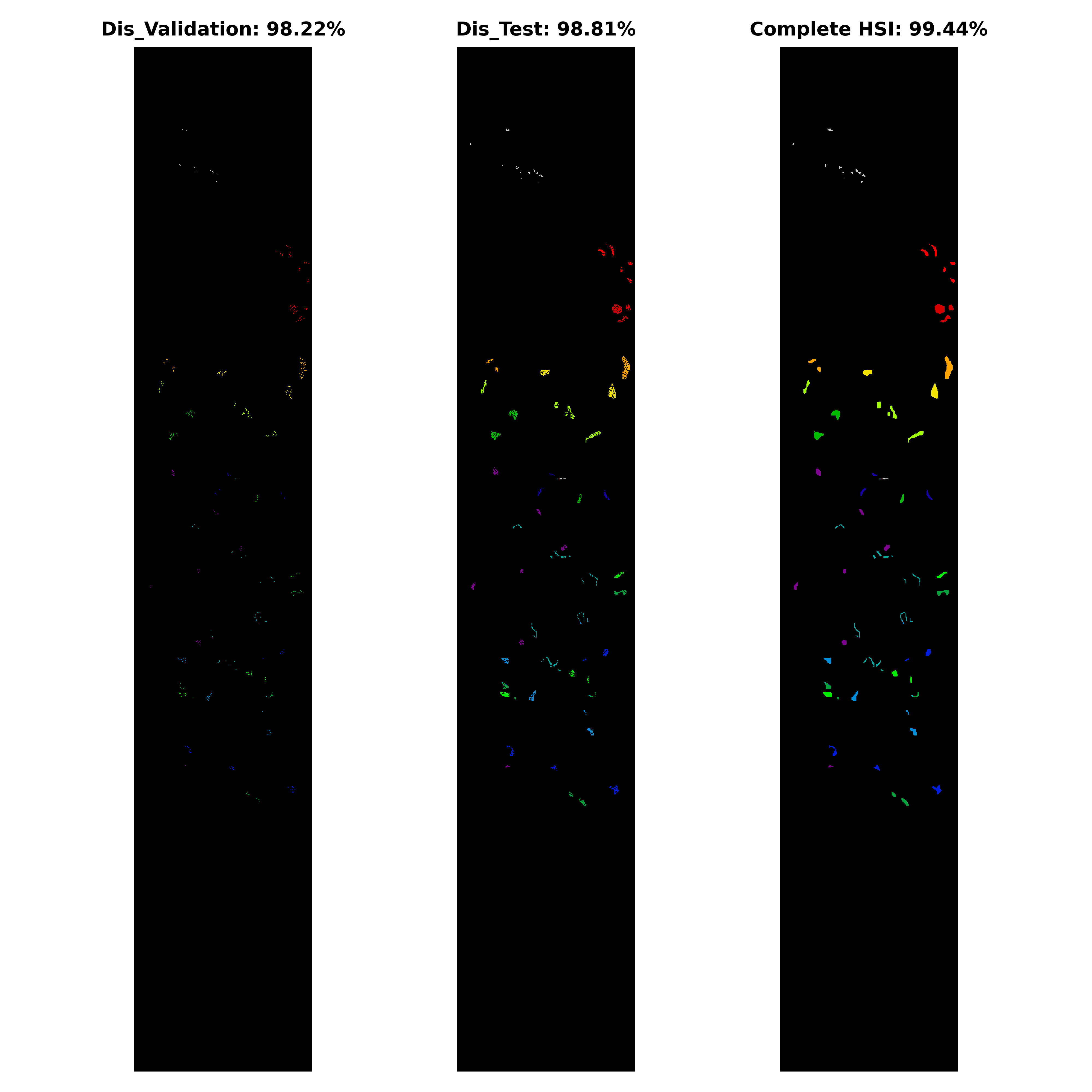
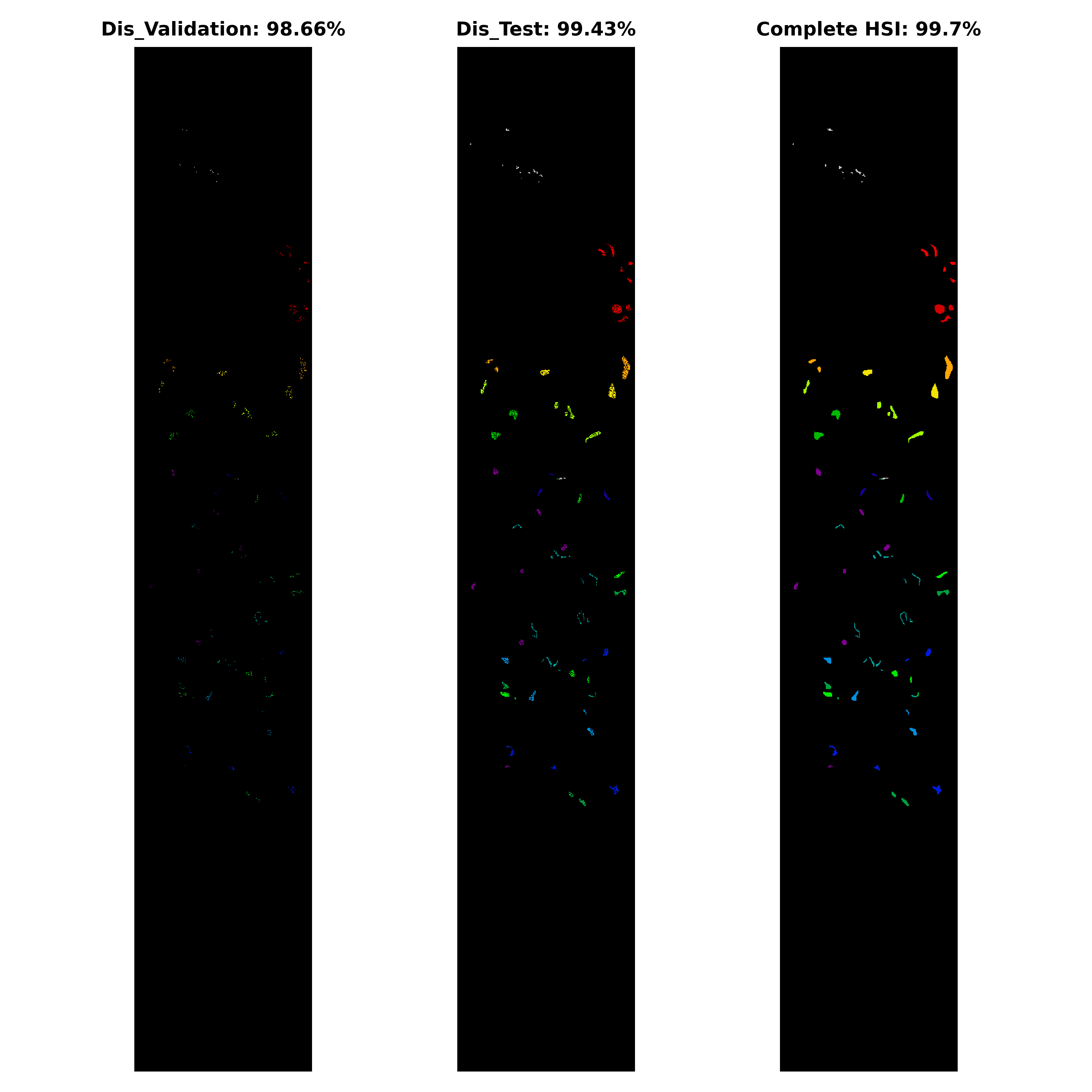
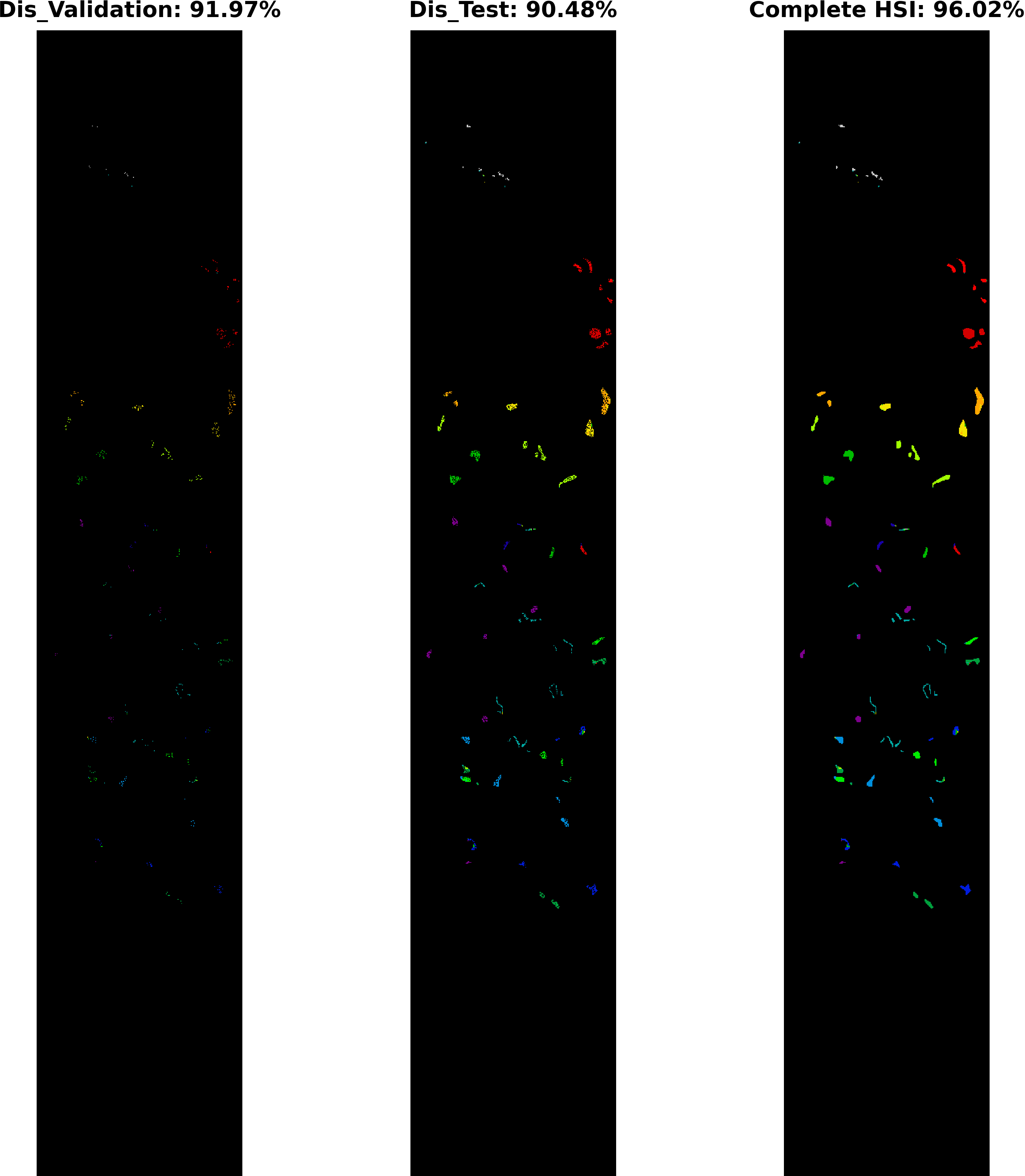
To ensure a robust and fair evaluation, the HSI datasets are split into disjoint training, validation, and test sets. Following the proposed method, we begin by dividing the HSI dataset into disjoint training, validation, and test sets. Each model is then trained on the training set and tuned on the validation set to optimize performance. Subsequently, the models are evaluated on the disjoint test set and the complete HSI dataset to assess their generalization capabilities. The experimental results demonstrate the effectiveness of the proposed method in improving the classification accuracy of HSIC as shown in Tables VI, VII, VIII, IX, and X and Figures 8, 9, 10, 11, and 12. Among the deep learning models considered, 3D CNN [19] and Hybrid Inception Net [37] achieve the highest classification accuracy, indicating their suitability for HSIC. Additionally, the results highlight the importance of using a large and diverse training dataset to achieve optimal performance.

The comparative methods frequently misclassify samples with similar spatial structures, exemplified by the misclassification of Meadows and Bare Soil classes in the Pavia University dataset, as illustrated in Figure 9. Furthermore, the overall accuracy (OA) for the Grapes Untrained class is lower compared to other classes due to the aforementioned reasons as shown in Table VII. In summary, higher accuracy can be attained by employing a greater number of labeled samples (complete HSI dataset as the test set), as depicted in Figures 8, 9, 10, 11, and 12 and Tables VI, VII, VIII, IX, and X, nevertheless, the elevated accuracy is accompanied by the drawbacks of bias, redundancy, and diminished generalization performance. Tables VI, VII, VIII, IX, and X also illustrate the computational time required to process and evaluate the HSI datasets used in this study. As depicted in the Tables, the time exhibits a gradual increase with the growing number of samples, i.e., Disjoint validation, disjoint test, and complete HSI dataset as a test set.

IV Conclusion

This paper introduces a novel technique for generating disjoint train, validation, and test splits in Hyperspectral Image Classification (HSIC). By efficiently partitioning the ground truth data, the proposed technique guarantees unbiased performance evaluations and facilitates reliable comparisons between classification models. This technique serves as a valuable tool for generating disjoint splits, ensuring that the subsets are representative of the entire dataset and the classification results are not skewed due to data leakage. While the presented technique offers significant advantages, we acknowledge that there may be limitations and opportunities for further improvements. Future research could explore alternative strategies for data splitting that consider additional factors, such as class imbalance or spatial coherence, to enhance the representativeness and generalizability of the subsets. By addressing these aspects, we can strive to develop even more robust and effective data-splitting techniques for HSIC.

References

- [1] M. Ahmad, S. Shabbir, S. K. Roy, D. Hong, X. Wu, J. Yao, A. M. Khan, M. Mazzara, S. Distefano, and J. Chanussot, “Hyperspectral image classification—traditional to deep models: A survey for future prospects,” IEEE Journal of Selected Topics in Applied Earth Observations and Remote Sensing, 2021.
- [2] V. Lodhi, D. Chakravarty, and P. Mitra, “Hyperspectral imaging for earth observation: Platforms and instruments,” Journal of the Indian Institute of Science, vol. 98, pp. 429–443, 2018.
- [3] Y. Li, D. Hong, C. Li, J. Yao, and J. Chanussote, “Hd-net: High-resolution decoupled network for building footprint extraction via deeply supervised body and boundary decomposition,” ISPRS Journal of Photogrammetry and Remote Sensing, vol. 209, pp. 51–65, 2024.
- [4] B. Lu, P. D. Dao, J. Liu, Y. He, and J. Shang, “Recent advances of hyperspectral imaging technology and applications in agriculture,” Remote Sensing, vol. 12, no. 16, p. 2659, 2020.
- [5] T. Adão, J. Hruška, L. Pádua, J. Bessa, E. Peres, R. Morais, and J. J. Sousa, “Hyperspectral imaging: A review on uav-based sensors, data processing and applications for agriculture and forestry,” Remote sensing, vol. 9, no. 11, p. 1110, 2017.
- [6] C. Li, B. Zhang, D. Hong, J. Yao, and J. Chanussot, “Lrr-net: An interpretable deep unfolding network for hyperspectral anomaly detection,” IEEE Transactions on Geoscience and Remote Sensing, 2023.
- [7] E. Bedini, “The use of hyperspectral remote sensing for mineral exploration: A review,” Journal of Hyperspectral Remote Sensing, vol. 7, no. 4, pp. 189–211, 2017.
- [8] C. Weber, R. Aguejdad, X. Briottet, J. Avala, S. Fabre, J. Demuynck, E. Zenou, Y. Deville, M. S. Karoui, F. Z. Benhalouche et al., “Hyperspectral imagery for environmental urban planning,” in IGARSS 2018-2018 IEEE International Geoscience and Remote Sensing Symposium. IEEE, 2018, pp. 1628–1631.
- [9] M. B. Stuart, A. J. McGonigle, and J. R. Willmott, “Hyperspectral imaging in environmental monitoring: A review of recent developments and technological advances in compact field deployable systems,” Sensors, vol. 19, no. 14, p. 3071, 2019.
- [10] C. B. Pande and K. N. Moharir, “Application of hyperspectral remote sensing role in precision farming and sustainable agriculture under climate change: A review,” Climate Change Impacts on Natural Resources, Ecosystems and Agricultural Systems, pp. 503–520, 2023.
- [11] M. H. Khan, Z. Saleem, M. Ahmad, A. Sohaib, H. Ayaz, M. Mazzara, and R. A. Raza, “Hyperspectral imaging-based unsupervised adulterated red chili content transformation for classification: Identification of red chili adulterants,” Neural Computing and Applications, vol. 33, no. 21, pp. 14 507–14 521, 2021.
- [12] M. H. Khan, Z. Saleem, M. Ahmad, A. Sohaib, H. Ayaz, and M. Mazzara, “Hyperspectral imaging for color adulteration detection in red chili,” Applied Sciences, vol. 10, no. 17, p. 5955, 2020.
- [13] Z. Saleem, M. H. Khan, M. Ahmad, A. Sohaib, H. Ayaz, and M. Mazzara, “Prediction of microbial spoilage and shelf-life of bakery products through hyperspectral imaging,” IEEE Access, vol. 8, pp. 176 986–176 996, 2020.
- [14] M. H. F. Butt, H. Ayaz, M. Ahmad, J. P. Li, and R. Kuleev, “A fast and compact hybrid cnn for hyperspectral imaging-based bloodstain classification,” in 2022 IEEE Congress on Evolutionary Computation (CEC). IEEE, 2022, pp. 1–8.
- [15] M. Zulfiqar, M. Ahmad, A. Sohaib, M. Mazzara, and S. Distefano, “Hyperspectral imaging for bloodstain identification,” Sensors, vol. 21, no. 9, p. 3045, 2021.
- [16] H. Ayaz, M. Ahmad, M. Mazzara, and A. Sohaib, “Hyperspectral imaging for minced meat classification using nonlinear deep features,” Applied Sciences, vol. 10, no. 21, p. 7783, 2020.
- [17] H. Ayaz, M. Ahmad, A. Sohaib, M. N. Yasir, M. A. Zaidan, M. Ali, M. H. Khan, and Z. Saleem, “Myoglobin-based classification of minced meat using hyperspectral imaging,” Applied Sciences, vol. 10, no. 19, p. 6862, 2020.
- [18] D. Hong, B. Zhang, X. Li, Y. Li, C. Li, J. Yao, N. Yokoya, H. Li, P. Ghamisi, X. Jia, A. Plaza, P. Gamba, J. A. Benediktsson, and J. Chanussot, “Spectralgpt: Spectral remote sensing foundation model,” IEEE Transactions on Pattern Analysis and Machine Intelligence, 2024, dOI:10.1109/TPAMI.2024.3362475.
- [19] M. Ahmad, A. M. Khan, M. Mazzara, S. Distefano, M. Ali, and M. S. Sarfraz, “A fast and compact 3-d cnn for hyperspectral image classification,” IEEE Geoscience and Remote Sensing Letters, 2020.
- [20] D. Hong, L. Gao, J. Yao, B. Zhang, A. Plaza, and J. Chanussot, “Graph convolutional networks for hyperspectral image classification,” IEEE Transactions on Geoscience and Remote Sensing, vol. 59, no. 7, pp. 5966–5978, 2021.
- [21] A. Jamali, S. K. Roy, D. Hong, P. M. Atkinson, and P. Ghamisi, “Attention graph convolutional network for disjoint hyperspectral image classification,” IEEE Geoscience and Remote Sensing Letters, pp. 1–1, 2024.
- [22] J. Yao, B. Zhang, C. Li, D. Hong, and J. Chanussot, “Extended vision transformer (exvit) for land use and land cover classification: A multimodal deep learning framework,” IEEE Transactions on Geoscience and Remote Sensing, 2023.
- [23] M. Ahmad, U. Ghous, M. Usama, and M. Mazzara, “Waveformer: Spectral–spatial wavelet transformer for hyperspectral image classification,” IEEE Geoscience and Remote Sensing Letters, 2024.
- [24] M. Ahmad, “Sharpend cosine similarity based neural network for hyperspectral image classification,” arXiv preprint arXiv:2305.16682, 2023.
- [25] ——, “Ground truth labeling and samples selection for hyperspectral image classification,” Optik, vol. 230, p. 166267, 2021. [Online]. Available: https://www.sciencedirect.com/science/article/pii/S0030402621000103
- [26] M. Ahmad, A. K. Bashir, and A. M. Khan, “Metric similarity regularizer to enhance pixel similarity performance for hyperspectral unmixing,” Optik, vol. 140, pp. 86–95, 2017. [Online]. Available: https://www.sciencedirect.com/science/article/pii/S003040261730311X
- [27] M. Ahmad, U. Ghous, D. Hong, A. M. Khan, J. Yao, S. Wang, and J. Chanussot, “A disjoint samples-based 3d-cnn with active transfer learning for hyperspectral image classification,” IEEE Transactions on Geoscience and Remote Sensing, vol. 60, pp. 1–16, 2022.
- [28] C. Geiß, P. Aravena Pelizari, H. Schrade, A. Brenning, and H. Taubenböck, “On the effect of spatially non-disjoint training and test samples on estimated model generalization capabilities in supervised classification with spatial features,” IEEE Geoscience and Remote Sensing Letters, vol. 14, no. 11, pp. 2008–2012, 2017.
- [29] M. Ahmad, A. Khan, A. M. Khan, M. Mazzara, S. Distefano, A. Sohaib, and O. Nibouche, “Spatial prior fuzziness pool-based interactive classification of hyperspectral images,” Remote Sensing, vol. 11, no. 9, p. 1136, 2019.
- [30] P. Zhang, H. Yu, P. Li, and R. Wang, “Transhsi: A hybrid cnn-transformer method for disjoint sample-based hyperspectral image classification,” Remote Sensing, vol. 15, no. 22, 2023.
- [31] D. Hong, C. Li, B. Zhang, N. Yokoya, J. A. Benediktsson, and J. Chanussot, “Multimodal artificial intelligence foundation models: Unleashing the power of remote sensing big data in earth observation,” The Innovation Geoscience, vol. 2, no. 1, p. 100055, 2024.
- [32] D. Hong, B. Zhang, H. Li, Y. Li, J. Yao, C. Li, M. Werner, J. Chanussot, A. Zipf, and X. X. Zhu, “Cross-city matters: A multimodal remote sensing benchmark dataset for cross-city semantic segmentation using high-resolution domain adaptation networks,” Remote Sensing of Environment, vol. 299, p. 113856, 2023.
- [33] J. Yao, X. Cao, D. Hong, X. Wu, D. Meng, J. Chanussot, and Z. Xu, “Semi-active convolutional neural networks for hyperspectral image classification,” IEEE Transactions on Geoscience and Remote Sensing, vol. 60, pp. 1–15, 2022.
- [34] U. Ghous, M. S. Sarfraz, M. Ahmad, C. Li, and D. Hong, “(2+1)d extreme xception net for hyperspectral image classification,” IEEE Journal of Selected Topics in Applied Earth Observations and Remote Sensing, pp. 1–14, 2024.
- [35] S. K. Adari and S. Alla, Introduction to Machine Learning. Berkeley, CA: Apress, 2024, pp. 105–134.
- [36] S. K. Roy, G. Krishna, S. R. Dubey, and B. B. Chaudhuri, “Hybridsn: Exploring 3-d–2-d cnn feature hierarchy for hyperspectral image classification,” IEEE Geoscience and Remote Sensing Letters, vol. 17, no. 2, pp. 277–281, 2020.
- [37] H. Fırat, M. E. Asker, M. İ. Bayındır, and D. Hanbay, “Hybrid 3d/2d complete inception module and convolutional neural network for hyperspectral remote sensing image classification,” Neural Processing Letters, vol. 55, no. 2, pp. 1087–1130, 2023.
- [38] X. Zhang, “Improved three-dimensional inception networks for hyperspectral remote sensing image classification,” IEEE Access, vol. 11, pp. 32 648–32 658, 2023.
- [39] Z. Xiong, Y. Yuan, and Q. Wang, “Ai-net: Attention inception neural networks for hyperspectral image classification,” in IGARSS 2018-2018 IEEE International Geoscience and Remote Sensing Symposium. IEEE, 2018, pp. 2647–2650.
- [40] X. Wu, D. Hong, and J. Chanussot, “Convolutional neural networks for multimodal remote sensing data classification,” IEEE Transactions on Geoscience and Remote Sensing, vol. 60, pp. 1–10, 2022.
- [41] S. Ghaderizadeh, D. Abbasi-Moghadam, A. Sharifi, N. Zhao, and A. Tariq, “Hyperspectral image classification using a hybrid 3d-2d convolutional neural networks,” IEEE Journal of Selected Topics in Applied Earth Observations and Remote Sensing, vol. 14, pp. 7570–7588, 2021.
- [42] X. Yang, Y. Ye, X. Li, R. Y. Lau, X. Zhang, and X. Huang, “Hyperspectral image classification with deep learning models,” IEEE Transactions on Geoscience and Remote Sensing, vol. 56, no. 9, pp. 5408–5423, 2018.