One-Pass Randomized Algorithm with Practical Rangefinder for Low-Rank Approximation to Quaternion Matrices

Chao Chang    Yuning Yang College of Mathematics and Information Science, Guangxi University, Nanning, 530004, ChinaCorresponding author: Yuning Yang, yyang@gxu.edu.cn.
Abstract

As its real/complex counterparts, randomized algorithms for low-rank approximation to quaternion matrices received attention recently. For large-scale problems, however, existing quaternion orthogonalization methods are not efficient, leading to slow rangefinders. By relaxing orthonormality while maintaining favaroable condition numbers, this work proposes two practical quaternion rangefinders that take advantage of mature scientific computing libraries to accelerate heavy computations. They are then incorporated into the quaternion version of a well-known one-pass algorithm. Theoretically, we establish the probabilistic error bound, and demonstrate that the error is proportional to the condition number of the rangefinder. Besides Gaussian, we also allow quaternion sub-Gaussian test matrices. Key to the latter is the derivation of a deviation bound for extreme singular values of a quaternion sub-Gaussian matrix. Numerical experiments indicate that the one-pass algorithm with the proposed rangefinders work efficiently while only sacrificing little accuracy. In addition, we tested the algorithm in an on-the-fly 3D Navier-Stokes equation data compression to demonstrate its efficiency in large-scale applications.

Keywords: Randomized Algorithm, Rangefinder, One-pass, Quaternion matrix, Sketching, Low-rank approximation, sub-Gaussian

1 Introduction

1.1 Background

Low-rank matrix approximation (LRMA) has been applied in various applications. In the big data era, large amounts of data are being captured and generated through various channels, such as high-definition color video, scientific simulations, and artificial intelligence training sets. This trend poses challenges in terms of computation time, storage, and memory costs to LRMA. In 2011, a randomized SVD algorithm (HMT) [14] was proposed by Halko, Martinsson, and Tropp, which uses a random sketch to obtain an oversampling approximation before implementing the truncated SVD. Compared to the deterministic SVD, the randomized one runs faster with adjustable precision loss. It is robust, but there is still a need to revisit the original data during the low-rank approximation. In 2017, Tropp et al. [41] proposed a one-pass randomized algorithm using two sketches, which needs to visit the data only once. It is more effective for managing data with limited storage, arithmetic, and communication capabilities. Later on, the authors developed also a one-pass algorithm using three sketches and applied it to streaming data [42]. Prior to these work, randomized algorithms have been studied extensively in the literature; see, e.g., [1, 46, 8, 30, 45, 9, 4], and the recent surveys [40, 20, 21, 34, 31, 32].

Despite the noncummutativity in quaternion multiplications, quaternion matrices have been widely used in various applications such as signal processing [11], color image analysis [39, 38], and machine learning [48, 33] in recent years. Randomized quaternion low-rank matrix approximation has garnered increasing attention very recently. Liu et al. [27] developed a randomized quaternion SVD algorithm based on the HMT framework by using structure-preserving quaternion QR and quaternion SVD, and studied its error bound. This algorithm was later applied to nonnegative pure quaternion matrix approximation [29]. Ren et al. [35] proposed a randomized quaternion QLP decomposition algorithm. Li et al. [23] also proposed a randomized block Krylov subspace algorithm with improved approximation accuracy. Very recently, a fixed-precesion randomized quaternion SVD was studied in [28].

The framework of the HMT algorithm [14] (also [41, 42], and the quaternion randomized algorithms [27, 35, 23]) can be divided into a randomized QB approximation stage and a truncation stage. Initially, the QB stage involves generating a sketch of the input data matrix through randomized oversampling with Gaussian or alternative embeddings. This then leads to the formation of the Q𝑄Q matrix, representing an orthonormal basis for the range of the sketch, known as the rangefinder step. The B𝐵B matrix is then determined, either exactly [14] or approximately [41, 42]. In the truncation stage, truncated SVD or other deterministic methods are performed on the B𝐵B matrix to find a more accurate fixed-rank approximation.

1.2 Quaternion rangefinders

In the real/complex case, constructing an orthonormal rangefinder is cheap. Fast and stable algorithms for orthogonalization have matured, and highly optimized implementations are available, such as MATLAB’s built-in function qr, and various QR routines in LAPACK [3] and the Intel Math Kernel Library (MKL) [10].

In the quaternion case, orthogonalization approaches are developing. Classical QR decomposition methods can be extended to the quaternion arithmetic with little modifications. For example, the quaternionic Householder QR was proposed for quaternion eigenvalue computations [5]; this was implemented by Sangwine and Le Bihan in the quaternion toolbox for MATLAB (QTFM) [36] with the function name qr. To speed up quaternion matrix computations, in a series of papers [18, 24, 19, 7], the authors proposed structure-preserving algorithms. This type of algorithms is promising, as its basic idea is to only operate on the compact real representation of a quaternion matrix, avoiding quaternion operations and smartly reducing computational complexity. The structure-preserving quaternion Householder QR (QHQR) [19, 26] is numerically stable and accurate; the structure-preserving quaternionic modified Gram-Schimit (QMGS) [44] is more economic but may lose accuracy. These methods together with QTFM’s qr function were employed for orthonormal rangefinders by the quaternion randomized algorithms [27, 23, 35].

1.3 Limitation and motivation
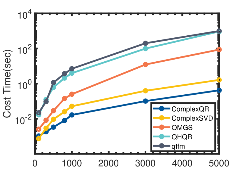
Refer to caption
Figure 1: Running time comparisons of QTFM’s qr, QHQR, QMGS, and MATLAB’s qr and svd (applied to the full complex representation). m𝑚m from 100100100 to 500050005000, n=0.1m𝑛0.1𝑚n=0.1m

The above quaternionic orthogonalization methods are efficient in small and moderate problems; however, for large-scale matrices, they are still expensive. For instance, even QMGS (wihch is the fastest one mentioned in the previous subsection) is at least two order of magnitude slower than qr in MATLAB for 5000×50050005005000\times 500 matrices; see Fig. 1111The code of QHQR was downloaded from http://maths.jsnu.edu.cn/_upload/article/files/40/5c/0abecd234d2c909be8b4fac9c4ad/1f0499ce-65d1-4364-9000-b8998137e516.zip and that of QMGS was implemented from [2]. MATLAB’s qr and svd are applied to the full complex representation of the quaternion matrix, which is of size 2m×0.2m2𝑚0.2𝑚2m\times 0.2m; see the next section. As complex QR and SVD cannot directly generate an orthonormal rangefinder in the quaternion domain, the purpose of this rough comparison is to show that the speed of computing the rangefinder still has a large room to improve.. One of the possible reasons is that highly optimized implementations of these quaternion orthogonalization methods are far from developed. For example, MATLAB’s built-in functions such as qr and svd do not support quaternions yet; nor MKL. Without an elegant implementation, even an advanced method cannot take advantage of the features such as parallelism and memory management in modern computing architecture, holding back its advancement.

To pursue speed, a common design philosophy is to trade accuracy, akin to randomized algorithms. Following this vein, it is possible to consider a non-orthonormal rangefinder. If so, what criteria should the new rangefinder meet, and how to quantify the loss of orthonormality?

Within the HMT and RQSVD frameworks, the orthonormal rangefinder plays two roles. One is to improve the numerical stability in matrix decompositions [14, Section 4.1]. The other is to explode the singular values and their corresponding singular vectors in the truncation stage, which helps in better approximating the original matrix. To quantify the accuracy, it is natural to take the condition number of the rangefinder into account. Obviously, an orthonormal rangefinder gives the optimal condition number, while deviations from orthonormality should maintain a condition number that does not indicate severe ill-conditioning.

When the criterion above is met, it is expected that the new rangefinder is built upon mature scientific computing libraries or advanced algorithms in the real/complex arithmetic to fully utilize the modern computing architecture.

1.4 This work

The general idea throughout this work is to transform heavy quaternion computations to QR, SVD, and solving linear equations in the complex arithmetic. To this end, we employ compact or full complex representations of quaternion matrices as intermediaries, accepting potential reductions in orthonormality and accuracy to maintain favorable condition numbers. The influence of condition numbers on approximation accuracy will be examined theoretically. Specifically:

In Section 3, we provide two range-preserving rangefinders, termed pseudo-QR and pseudo-SVD. Theoretically, Pseudo-QR can reduce the condition number of the sketch from 108superscript10810^{8} within 101010. Pseudo-SVD on the other hand generates an orthonormal matrix even with very ill-conditioned sketch. Almost all the computations are built upon established scientific computing libraries in the complex arithmetic to ensure their efficiency.

In Section 4, the proposed rangefinders are incorporated into the quaternion version of the one-pass framework of [41].

Our theoretical findings in Sections 4, 5, and 6 are summarized as follows:

  • In the QB approximation stage, the approximation error, measured by the tail energy, is independent of the condition number of the rangefinder;

  • In the truncation stage, the truncation error is proportional to the condition number of the rangefinder. This and the previous point ensure the reasonability of using a non-orthonormal yet well-conditioned rangefinder in theory.

  • We derive a deviation bound for extreme singular values of a quaternion sub-Gaussian matrix, which may be of independent interest. This theoretically justifies the use of quaternion sub-Gaussian test matrices.

Some comments are in order.

  • The result of the first two points applies to any range-preserving while non-orthonormal rangefinders.

  • The deviation bound of extreme singular values of a quaternion Gaussian matrix was first studied in [27], while ours in the sub-Gaussian case generalizes a result in the real case by Vershynin [43]. Specifically, with high probability, the singular values of a tall m×n𝑚𝑛m\times n quaternion sub-Gaussian matrix are shown to lie in the interval [2m2Cnt,2m+2Cn+t]2𝑚2𝐶𝑛𝑡2𝑚2𝐶𝑛𝑡[2\sqrt{m}-2C\sqrt{n}-t,2\sqrt{m}+2C\sqrt{n}+t] for some C,t>0𝐶𝑡0C,t>0.

Finally, Section 7 evaluates the performance of our algorithm and other ones through various experiments using synthetic data. We apply our method to compression of scientific simulation data from 3D Navier-Stokes equations and a 4D Lorenz-type chaotic system to demonstrate its efficiency in large-scale problems.

Our implementation in MATLAB is available at github.com/Mitchell-Cxyk/RQLRMA, which can be ran with either CPU or GPU.

2 Preliminaries on Quaternions

Quaternions were invented by Sir William Rowan Hamilton in 1843. A quaternion scalar is of the form a=aw+ax𝐢+ay𝐣+az𝐤𝑎subscript𝑎𝑤subscript𝑎𝑥𝐢subscript𝑎𝑦𝐣subscript𝑎𝑧𝐤a=a_{w}+a_{x}\mathbf{i}+a_{y}\mathbf{j}+a_{z}\mathbf{k} where aw,ax,ay,azsubscript𝑎𝑤subscript𝑎𝑥subscript𝑎𝑦subscript𝑎𝑧a_{w},a_{x},a_{y},a_{z} are real numbers. The sum of quaternions is defined component-wise and the their multiplication is determined by the following rules along with the associative and distributive laws 𝐢2=𝐣2=𝐤2=𝐢𝐣𝐤=1superscript𝐢2superscript𝐣2superscript𝐤2𝐢𝐣𝐤1\mathbf{i}^{2}=\mathbf{j}^{2}=\mathbf{k}^{2}=\mathbf{i}\mathbf{j}\mathbf{k}=-1. For a,b𝑎𝑏a,b\in\mathbb{Q}, abba𝑎𝑏𝑏𝑎ab\neq ba in general. A quaternion matrix 𝐐m×n𝐐superscript𝑚𝑛\mathbf{Q}\in\mathbb{Q}^{m\times n} is defined as 𝐐=Qw+Qx𝐢+Qy𝐣+Qz𝐤𝐐subscript𝑄𝑤subscript𝑄𝑥𝐢subscript𝑄𝑦𝐣subscript𝑄𝑧𝐤\mathbf{Q}=Q_{w}+Q_{x}\mathbf{i}+Q_{y}\mathbf{j}+Q_{z}\mathbf{k}, where Qi(i=w,x,y,z)m×nsubscript𝑄𝑖𝑖𝑤𝑥𝑦𝑧superscript𝑚𝑛Q_{i}(i=w,x,y,z)\in\mathbb{R}^{m\times n}. The conjugate and conjugate transpose of 𝐐𝐐\mathbf{Q} are respectively denoted as 𝐐¯:=QwQx𝐢Qy𝐣Qz𝐤assign¯𝐐subscript𝑄𝑤subscript𝑄𝑥𝐢subscript𝑄𝑦𝐣subscript𝑄𝑧𝐤\overline{\mathbf{Q}}:=Q_{w}-Q_{x}\mathbf{i}-Q_{y}\mathbf{j}-Q_{z}\mathbf{k} and 𝐐:=QwTQxT𝐢QyT𝐣QzT𝐤assignsuperscript𝐐superscriptsubscript𝑄𝑤𝑇superscriptsubscript𝑄𝑥𝑇𝐢superscriptsubscript𝑄𝑦𝑇𝐣superscriptsubscript𝑄𝑧𝑇𝐤\mathbf{Q}^{*}:=Q_{w}^{T}-Q_{x}^{T}\mathbf{i}-Q_{y}^{T}\mathbf{j}-Q_{z}^{T}\mathbf{k}. For two quaternion matrices 𝐏𝐏\mathbf{P} and 𝐐𝐐\mathbf{Q} of proper size, 𝐏𝐐=(𝐐𝐏)superscript𝐏𝐐superscriptsuperscript𝐐𝐏\mathbf{P}^{*}\mathbf{Q}=(\mathbf{Q}^{*}\mathbf{P})^{*} while 𝐏𝐐¯𝐏¯𝐐¯¯superscript𝐏𝐐¯superscript𝐏¯𝐐\overline{\mathbf{P}^{*}\mathbf{Q}}\neq\overline{\mathbf{P}^{*}}\cdot\overline{\mathbf{Q}}. More properties are referred to [47].

2.1 Quaternion vector space

Considering vectors with quaternion coordinates, a module over the ring \mathbb{Q} is usually called the quaternion right vector space under the summation and the right scalar multiplication. Given quaternion vectors 𝐯1,,𝐯rsubscript𝐯1subscript𝐯𝑟\mathbf{v}_{1},\ldots,\mathbf{v}_{r}, they are right linearly independent if for quaternions k1,,krsubscript𝑘1subscript𝑘𝑟k_{1},\ldots,k_{r},

𝐯1k1+𝐯2k2++𝐯rkr=0implieski=0,i=1,,r.formulae-sequencesubscript𝐯1subscript𝑘1subscript𝐯2subscript𝑘2subscript𝐯𝑟subscript𝑘𝑟0impliesformulae-sequencesubscript𝑘𝑖0𝑖1𝑟\displaystyle\mathbf{v}_{1}k_{1}+\mathbf{v}_{2}k_{2}+\cdots+\mathbf{v}_{r}k_{r}=0\quad\text{implies}\quad k_{i}=0,~{}~{}i=1,\ldots,r.

Most linear algebra concepts and results can be transplanted to the right vector space in parallel [47] and throughout this work, we always omit the prefix “right”.

Given 𝐕=[𝐯1,,𝐯r]𝐕subscript𝐯1subscript𝐯𝑟\mathbf{V}=[\mathbf{v}_{1},\ldots,\mathbf{v}_{r}], its range is defined as

(𝐕)=span(𝐯1,,𝐯r)={i=1r𝐯ikrkr,i=1,,r}.𝐕spansubscript𝐯1subscript𝐯𝑟conditional-setsubscriptsuperscript𝑟𝑖1subscript𝐯𝑖subscript𝑘𝑟formulae-sequencesubscript𝑘𝑟𝑖1𝑟{\mathcal{R}}(\mathbf{V})={\rm span}(\mathbf{v}_{1},\ldots,\mathbf{v}_{r})=\left\{\sum^{r}_{i=1}\nolimits\mathbf{v}_{i}k_{r}~{}\mid~{}k_{r}\in\mathbb{Q},~{}i=1,\ldots,r\right\}.

The inner product between 𝐮𝐮\mathbf{u} and 𝐯𝐯\mathbf{v} is given by 𝐮,𝐯=𝐮𝐯𝐮𝐯superscript𝐮𝐯\langle\mathbf{u},\mathbf{v}\rangle=\mathbf{u}^{*}\mathbf{v} [17, 6]. They are orthogonal if 𝐮,𝐯=0𝐮𝐯0\langle\mathbf{u},\mathbf{v}\rangle=0 and written as 𝐮𝐯perpendicular-to𝐮𝐯\mathbf{u}\perp\mathbf{v}. If 𝐮,𝐮=𝐯,𝐯=1𝐮𝐮𝐯𝐯1\langle\mathbf{u},\mathbf{u}\rangle=\langle\mathbf{v},\mathbf{v}\rangle=1, they are called orthonormal quaternion vectors. Considering a quaternion linear space 𝒱𝒱\mathcal{V}, for a subspace 𝒱𝒱\mathcal{L}\subset\mathcal{V}, its orthogonal complement is defined as ={𝐯𝒱:𝐯,𝐰=0,𝐰}superscriptbottomconditional-set𝐯𝒱formulae-sequence𝐯𝐰0for-all𝐰\mathcal{L}^{\bot}=\{\mathbf{v}\in\mathcal{V}:\langle\mathbf{v},\mathbf{w}\rangle=0,\forall\mathbf{w}\in\mathcal{L}\}.

2.2 Complex representation

𝐐m×n𝐐superscript𝑚𝑛\mathbf{Q}\in\mathbb{Q}^{m\times n} can be represented as 𝐐=Q0+Q1𝐣𝐐subscript𝑄0subscript𝑄1𝐣\mathbf{Q}=Q_{0}+Q_{1}\mathbf{j}, where Q0,Q1m×nsubscript𝑄0subscript𝑄1superscript𝑚𝑛Q_{0},Q_{1}\in\mathbb{C}^{m\times n} with Q0=Qw+Qx𝐢subscript𝑄0subscript𝑄𝑤subscript𝑄𝑥𝐢Q_{0}=Q_{w}+Q_{x}\mathbf{i} and Q1=Qy+Qz𝐢subscript𝑄1subscript𝑄𝑦subscript𝑄𝑧𝐢Q_{1}=Q_{y}+Q_{z}\mathbf{i}. The (full) complex representation of 𝐐𝐐\mathbf{Q} is defined as [47]:

χ𝐐:=[Q0Q1Q1¯Q0¯]2m×2n.assignsubscript𝜒𝐐matrixsubscript𝑄0subscript𝑄1¯subscript𝑄1¯subscript𝑄0superscript2𝑚2𝑛\displaystyle{\chi}_{\mathbf{Q}}:=\begin{bmatrix}Q_{0}&Q_{1}\\ -\overline{Q_{1}}&\overline{Q_{0}}\end{bmatrix}\in\mathbb{C}^{2m\times 2n}.

χ𝐐subscript𝜒𝐐{\chi}_{\mathbf{Q}} has several nice properties that it is useful in the study of quaternions:

Proposition 2.1 ([47]).

Let 𝐏,𝐐𝐏𝐐\mathbf{P},\mathbf{Q} be quaternion matrices of proper size. Then

χk1𝐏+k2𝐐=k1χ𝐏+k2χ𝐐(k1,k2),χ𝐏𝐐=χ𝐏χ𝐐,formulae-sequencesubscript𝜒subscript𝑘1𝐏subscript𝑘2𝐐subscript𝑘1subscript𝜒𝐏subscript𝑘2subscript𝜒𝐐subscript𝑘1subscript𝑘2subscript𝜒𝐏𝐐subscript𝜒𝐏subscript𝜒𝐐\displaystyle{\chi}_{k_{1}\mathbf{P}+k_{2}\mathbf{Q}}=k_{1}{\chi}_{\mathbf{P}}+k_{2}{\chi}_{\mathbf{Q}}(k_{1},k_{2}\in\mathbb{R}),\quad{\chi}_{\mathbf{P}\mathbf{Q}}={\chi}_{\mathbf{P}}{\chi}_{\mathbf{Q}},
χ𝐐=χ𝐐,χ𝐐1=χ𝐐1if𝐐1exists,formulae-sequencesubscript𝜒superscript𝐐superscriptsubscript𝜒𝐐subscript𝜒superscript𝐐1superscriptsubscript𝜒𝐐1ifsuperscript𝐐1exists\displaystyle{\chi}_{\mathbf{Q}^{*}}={\chi}_{\mathbf{Q}}^{*},\quad{\chi}_{\mathbf{Q}^{-1}}={\chi}_{\mathbf{Q}}^{-1}~{}{\rm if}~{}\mathbf{Q}^{-1}~{}{\rm exists},
χ𝐐is(partially)unitary/Hermitianifandonlyif𝐐is(partially)unitary/Hemitian.subscript𝜒𝐐ispartiallyunitaryHermitianifandonlyif𝐐ispartiallyunitaryHemitian\displaystyle{\chi}_{\mathbf{Q}}~{}{\rm is~{}(partially)~{}unitary/Hermitian~{}if~{}and~{}only~{}if}~{}\mathbf{Q}~{}{\rm is~{}(partially)~{}unitary/Hemitian}.

χ𝐐subscript𝜒𝐐{\chi}_{\mathbf{Q}} can be partitioned as two blocks:

χ𝐐=[𝐐c,𝐐a],with𝐐c:=[Q0Q1¯],𝐐a:=[Q1Q0¯].formulae-sequencesubscript𝜒𝐐subscript𝐐𝑐subscript𝐐𝑎formulae-sequenceassignwithsubscript𝐐𝑐matrixsubscript𝑄0¯subscript𝑄1assignsubscript𝐐𝑎matrixsubscript𝑄1¯subscript𝑄0\displaystyle{\chi}_{\mathbf{Q}}=[\mathbf{Q}_{c},\mathbf{Q}_{a}],~{}{\rm with}~{}\mathbf{Q}_{c}:=\begin{bmatrix}Q_{0}\\ -\overline{Q_{1}}\end{bmatrix},~{}\mathbf{Q}_{a}:=\begin{bmatrix}Q_{1}\\ \overline{Q_{0}}\end{bmatrix}.

We call 𝐐csubscript𝐐𝑐\mathbf{Q}_{c} the compact complex representation of 𝐐𝐐\mathbf{Q}. 𝐐asubscript𝐐𝑎\mathbf{Q}_{a} can be generated from 𝐐csubscript𝐐𝑐\mathbf{Q}_{c} by using the symplectic matrix 𝒥:=[0ImIm0]assign𝒥matrix0subscript𝐼𝑚subscript𝐼𝑚0\mathcal{J}:=\begin{bmatrix}0&-I_{m}\\ I_{m}&0\end{bmatrix}, with 𝐐a=𝒥𝐐c¯subscript𝐐𝑎𝒥¯subscript𝐐𝑐\mathbf{Q}_{a}=\mathcal{J}\overline{\mathbf{Q}_{c}}. The relation between 𝐐csubscript𝐐𝑐\mathbf{Q}_{c} and 𝐐asubscript𝐐𝑎\mathbf{Q}_{a} is important in the design and analysis of our rangefinders. One can directly check that 𝒥𝒥\mathcal{J} admits the following properties:

Lemma 2.1.

J-adjoint satisfies:

𝒥=𝒥1=𝒥;χ𝐐=[𝐐c,𝒥𝐐c¯];𝒥χ𝐐𝒥=𝒥χ𝐐𝒥=χ𝐐¯;formulae-sequencesuperscript𝒥superscript𝒥1𝒥formulae-sequencesubscript𝜒𝐐subscript𝐐𝑐𝒥¯subscript𝐐𝑐superscript𝒥subscript𝜒𝐐𝒥𝒥subscript𝜒𝐐superscript𝒥¯subscript𝜒𝐐\displaystyle\mathcal{J}^{*}=\mathcal{J}^{-1}=-\mathcal{J};\quad{\chi}_{\mathbf{Q}}=[\mathbf{Q}_{c},\mathcal{J}\overline{\mathbf{Q}_{c}}];\quad\mathcal{J}^{*}{\chi}_{\mathbf{Q}}\mathcal{J}=\mathcal{J}{\chi}_{\mathbf{Q}}\mathcal{J}^{*}=\overline{{\chi}_{\mathbf{Q}}};
𝒥[v,𝒥v¯]𝒥=𝒥[v,𝒥v¯]𝒥=[v,𝒥v¯]¯,andv,𝒥v¯=0,v2m.formulae-sequencesuperscript𝒥𝑣𝒥¯𝑣𝒥𝒥𝑣𝒥¯𝑣superscript𝒥¯𝑣𝒥¯𝑣and𝑣𝒥¯𝑣0for-all𝑣superscript2𝑚\displaystyle\mathcal{J}^{*}[v,\mathcal{J}\overline{v}]\mathcal{J}=\mathcal{J}[v,\mathcal{J}\overline{v}]\mathcal{J}^{*}=\overline{[v,\mathcal{J}\overline{v}]},\quad{\rm and}\quad\left\langle v,\mathcal{J}\overline{v}\right\rangle=0,\forall v\in\mathbb{C}^{2m}.

The quaternion Moore-Penrose (MP) inverse can be defined similarly as its real/complex counterpart [2, section 1.6]. For 𝐀m×n𝐀superscript𝑚𝑛\mathbf{A}\in\mathbb{Q}^{m\times n}, there exists a unique solution 𝐗𝐗\mathbf{X}, denoted as 𝐀superscript𝐀\mathbf{A}^{\dagger}, that satisfies the following four matrix equations

𝐀𝐗𝐀=𝐀,𝐗𝐀𝐗=𝐗,(𝐀𝐗)=𝐀𝐀𝐗,(𝐗𝐀)=𝐗𝐀.formulae-sequence𝐀𝐗𝐀𝐀formulae-sequence𝐗𝐀𝐗𝐗formulae-sequencesuperscript𝐀𝐗𝐀𝐀𝐗superscript𝐗𝐀𝐗𝐀\displaystyle\mathbf{A}\mathbf{X}\mathbf{A}=\mathbf{A},~{}~{}\mathbf{X}\mathbf{A}\mathbf{X}=\mathbf{X},~{}~{}(\mathbf{A}\mathbf{X})^{*}=\mathbf{A}\mathbf{A}\mathbf{X},~{}~{}(\mathbf{X}\mathbf{A})^{*}=\mathbf{X}\mathbf{A}.
Lemma 2.2.

Let 𝐀m×n𝐀superscript𝑚𝑛\mathbf{A}\in\mathbb{Q}^{m\times n}; then χ𝐀=(χ𝐀)subscript𝜒superscript𝐀superscriptsubscript𝜒𝐀\chi_{\mathbf{A}^{\dagger}}=\left(\chi_{\mathbf{A}}\right)^{\dagger}.

Proof.

The lemma can be proved by checking the MP inverse directly:

χ𝐀χ𝐀χ𝐀subscript𝜒superscript𝐀subscript𝜒𝐀subscript𝜒superscript𝐀\displaystyle{\chi}_{\mathbf{A}^{\dagger}}{\chi}_{\mathbf{A}}{\chi}_{\mathbf{A}^{\dagger}} =χ𝐀𝐀𝐀=χ𝐀,absentsubscript𝜒superscript𝐀superscript𝐀𝐀subscript𝜒superscript𝐀\displaystyle={\chi}_{\mathbf{A}^{\dagger}\mathbf{A}\mathbf{A}^{\dagger}}={\chi}_{\mathbf{A}^{\dagger}},
χ𝐀χ𝐀χ𝐀subscript𝜒𝐀subscript𝜒superscript𝐀subscript𝜒𝐀\displaystyle{\chi}_{\mathbf{A}}{\chi}_{\mathbf{A}^{\dagger}}{\chi}_{\mathbf{A}} =χ𝐀𝐀𝐀=χ𝐀,absentsubscript𝜒superscript𝐀𝐀𝐀subscript𝜒𝐀\displaystyle={\chi}_{\mathbf{A}\mathbf{A}^{\dagger}\mathbf{A}}={\chi}_{\mathbf{A}},
(χ𝐀χ𝐀)=χ𝐀𝐀superscriptsubscript𝜒𝐀subscript𝜒superscript𝐀subscriptsuperscript𝜒superscript𝐀𝐀\displaystyle\left({\chi}_{\mathbf{A}}{\chi}_{\mathbf{A}^{\dagger}}\right)^{*}={\chi}^{*}_{\mathbf{A}\mathbf{A}^{\dagger}} =χ(𝐀𝐀)=χ𝐀𝐀=χ𝐀χ𝐀,absentsubscript𝜒superscriptsuperscript𝐀𝐀subscript𝜒superscript𝐀𝐀subscript𝜒𝐀subscript𝜒superscript𝐀\displaystyle={\chi}_{(\mathbf{A}\mathbf{A}^{\dagger})^{*}}={\chi}_{\mathbf{A}\mathbf{A}^{\dagger}}={\chi}_{\mathbf{A}}{\chi}_{\mathbf{A}^{\dagger}},
(χ𝐀χ𝐀)=χ𝐀𝐀superscriptsubscript𝜒superscript𝐀subscript𝜒𝐀subscriptsuperscript𝜒superscript𝐀𝐀\displaystyle\left({\chi}_{\mathbf{A}^{\dagger}}{\chi}_{\mathbf{A}}\right)^{*}={\chi}^{*}_{\mathbf{A}^{\dagger}\mathbf{A}} =χ(𝐀𝐀)=χ𝐀𝐀=χ𝐀χ𝐀.absentsubscript𝜒superscriptsuperscript𝐀𝐀subscript𝜒superscript𝐀𝐀subscript𝜒superscript𝐀subscript𝜒𝐀\displaystyle={\chi}_{(\mathbf{A}^{\dagger}\mathbf{A})^{*}}={\chi}_{\mathbf{A}^{\dagger}\mathbf{A}}={\chi}_{\mathbf{A}^{\dagger}}{\chi}_{\mathbf{A}}.

Lemma 2.3.

Let U2m×n𝑈superscript2𝑚𝑛U\in\mathbb{C}^{2m\times n}; denote M:=[U,𝒥U¯]assign𝑀𝑈𝒥¯𝑈M:=[U,\mathcal{J}\overline{U}] and PM:=MMassignsubscript𝑃𝑀𝑀superscript𝑀P_{M}:=MM^{\dagger} the orthogonal projection on to (M)𝑀\mathcal{R}(M). Then 𝒥PM𝒥=𝒥PM𝒥=PM¯𝒥subscript𝑃𝑀superscript𝒥superscript𝒥subscript𝑃𝑀𝒥¯subscript𝑃𝑀\mathcal{J}P_{M}\mathcal{J}^{*}=\mathcal{J}^{*}P_{M}\mathcal{J}=\overline{P_{M}}.

Proof.

Denote 𝐔m×n𝐔superscript𝑚𝑛\mathbf{U}\in\mathbb{Q}^{m\times n} such that 𝐔c=Usubscript𝐔𝑐𝑈\mathbf{U}_{c}=U. Then χ𝐔=Msubscript𝜒𝐔𝑀{\chi}_{\mathbf{U}}=M. Thus

𝒥PM𝒥=𝒥χ𝐔χ𝐔𝒥=𝒥χ𝐔𝐔𝒥=χ𝐔𝐔¯=χ𝐔χ𝐔¯=MM¯=PM¯,𝒥subscript𝑃𝑀superscript𝒥𝒥subscript𝜒𝐔superscriptsubscript𝜒𝐔superscript𝒥𝒥subscript𝜒superscript𝐔𝐔superscript𝒥¯subscript𝜒superscript𝐔𝐔¯subscript𝜒𝐔superscriptsubscript𝜒𝐔¯𝑀superscript𝑀¯subscript𝑃𝑀\displaystyle\mathcal{J}P_{M}\mathcal{J}^{*}=\mathcal{J}{\chi}_{\mathbf{U}}{\chi}_{\mathbf{U}}^{\dagger}\mathcal{J}^{*}=\mathcal{J}{\chi}_{\mathbf{U}\mathbf{U}^{\dagger}}\mathcal{J}^{*}=\overline{{\chi}_{\mathbf{U}\mathbf{U}^{\dagger}}}=\overline{{\chi}_{\mathbf{U}}{\chi}_{\mathbf{U}}^{\dagger}}=\overline{MM^{\dagger}}=\overline{P_{M}},

where the second and fourth equalities are due to Lemma 2.2 and Proposition 2.1, and the third one comes from Lemma 2.1. Verifying 𝒥PM𝒥=PM¯superscript𝒥subscript𝑃𝑀𝒥¯subscript𝑃𝑀\mathcal{J}^{*}P_{M}\mathcal{J}=\overline{P_{M}} is similar. ∎

Analygously to the real/complex case, quaternion matrices admit SVD:

Theorem 2.1.

(compact QSVD [47, Theorem 7.2]) Let 𝐀m×n𝐀superscript𝑚𝑛\mathbf{A}\in\mathbb{Q}^{m\times n} (mn)𝑚𝑛(m\geq n) be of rank r𝑟r. Then there exists unitary quaternion matrices Um×m𝑈superscript𝑚𝑚U\in\mathbb{Q}^{m\times m}, Vn×n𝑉superscript𝑛𝑛V\in\mathbb{Q}^{n\times n} and diagonal real matrix Σ=diag(σ1,,σr,0,,0)n×nΣdiagsubscript𝜎1subscript𝜎𝑟00superscript𝑛𝑛\Sigma={\rm diag}(\sigma_{1},\ldots,\sigma_{r},0,\ldots,0)\in\mathbb{R}^{n\times n} with σ1σr>0subscript𝜎1subscript𝜎𝑟0\sigma_{1}\geq\cdots\geq\sigma_{r}>0, such that 𝐀=𝐔Σ𝐕𝐀𝐔Σsuperscript𝐕\mathbf{A}=\mathbf{U}\Sigma\mathbf{V}^{*}.

The following property, which can be deduced from [47], reveals the relation between the SVD of 𝐀m×n𝐀superscript𝑚𝑛\mathbf{A}\in\mathbb{Q}^{m\times n} and its complex representation χ𝐀subscript𝜒𝐀\chi_{\mathbf{A}}:

Proposition 2.2.

Under the notations in Theorem 2.1, if 𝐀=𝐔Σ𝐕𝐀𝐔Σsuperscript𝐕\mathbf{A}=\mathbf{U}\Sigma\mathbf{V}^{*}, then χ𝐀=χ𝐔Sχ𝐕subscript𝜒𝐀subscript𝜒𝐔𝑆superscriptsubscript𝜒𝐕{\chi}_{\mathbf{A}}={\chi}_{\mathbf{U}}S{\chi}_{\mathbf{V}}^{*} with S=diag(Σ,Σ)2n×2n𝑆diagΣΣsuperscript2𝑛2𝑛S={\rm diag}(\Sigma,\Sigma)\in\mathbb{R}^{2n\times 2n} is a compact SVD of χ𝐀subscript𝜒𝐀{\chi}_{\mathbf{A}}, and vice versa.

Lemma 2.4.

[2, Section 1.6] Under the notations in Theorem 2.1, if 𝐀=𝐔Σ𝐕𝐀𝐔Σsuperscript𝐕\mathbf{A}=\mathbf{U}\Sigma\mathbf{V}^{*}, then 𝐀=𝐔Σ𝐕superscript𝐀𝐔superscriptΣsuperscript𝐕\mathbf{A}^{\dagger}=\mathbf{U}\Sigma^{\dagger}\mathbf{V}^{*} with Σ=diag(σ11,,σr1,0,,0)n×nsuperscriptΣdiagsuperscriptsubscript𝜎11superscriptsubscript𝜎𝑟100superscript𝑛𝑛\Sigma^{\dagger}={\rm diag}(\sigma_{1}^{-1},\ldots,\sigma_{r}^{-1},0,\ldots,0)\in\mathbb{R}^{n\times n}.

3 Practical Quaternion Rangefinders

Given a data matrix A𝔽m×n𝐴superscript𝔽𝑚𝑛A\in\mathbb{F}^{m\times n} (𝔽=,,)𝔽(\mathbb{F}=\mathbb{R},\mathbb{C},\mathbb{Q}), a randomized rangefinder first draws a random test matrix Ω𝔽n×sΩsuperscript𝔽𝑛𝑠\Omega\in\mathbb{F}^{n\times s} with snmuch-less-than𝑠𝑛s\ll n [41] (s𝑠s is close to the target rank and often can be regarded as a constant), takes a sketch Y=AΩ𝑌𝐴ΩY=A\Omega, and then orthogonalizes it, i.e.,

Y=AΩ,Q=orth(Y),formulae-sequence𝑌𝐴Ω𝑄orth𝑌Y=A\Omega,~{}Q=\texttt{orth}(Y),

where Q𝑄Q is orthnormal and preserves the range of Y𝑌Y. In the real/complex case, computing Q𝑄Q is cheap by using QR decomposition, while things change in the quaternion setting, especially for large-scale problems, as discussed in the introduction. To better fit into the modern need, we present two practical rangefinders in this section by trading accuracy or space for time cost. To achieve this, we mostly employ mature libraries such as QR, SVD, and linear equation solvers in complex arithmetic for heavy computations. Finally, we will compare the running time of the proposed rangefinders with those in the literature.

3.1 Pseudo-QR

Given a quaternion matrix 𝐗=X0+X1𝐣m×n𝐗subscript𝑋0subscript𝑋1𝐣superscript𝑚𝑛\mathbf{X}=X_{0}+X_{1}\mathbf{j}\in\mathbb{Q}^{m\times n}, previous work (cite) indicates that full information has been contained in its compact represtation 𝐗c=[X0X1¯]2m×n,subscript𝐗𝑐matrixsubscript𝑋0¯subscript𝑋1superscript2𝑚𝑛\mathbf{X}_{c}=\begin{bmatrix}X_{0}\\ -\overline{X_{1}}\end{bmatrix}\in\mathbb{C}^{2m\times n}, while full representation χ𝐗subscript𝜒𝐗\chi_{\mathbf{X}} futher preserves its structure as an operator. Although Xcsubscript𝑋𝑐X_{c} does not capture the entire structure in the same way as χ𝐗subscript𝜒𝐗{\chi}_{\mathbf{X}}, the fact that χ𝐗subscript𝜒𝐗{\chi}_{\mathbf{X}} can be easily derived from 𝐗csubscript𝐗𝑐\mathbf{X}_{c} implies that underlying structure may still be preserved within 𝐗csubscript𝐗𝑐\mathbf{X}_{c}. Starting from this observation, we prefer to operate on 𝐗csubscript𝐗𝑐\mathbf{X}_{c} to obtain our first rangefinder.

Let 𝐘=𝐀𝛀=Y0+Y1𝐣m×s𝐘𝐀𝛀subscript𝑌0subscript𝑌1𝐣superscript𝑚𝑠\mathbf{Y}=\mathbf{A}\boldsymbol{\Omega}=Y_{0}+Y_{1}\mathbf{j}\in\mathbb{Q}^{m\times s} with m>s𝑚𝑠m>s be the sketch of the input data matrix 𝐀m×n𝐀superscript𝑚𝑛\mathbf{A}\in\mathbb{Q}^{m\times n}, with 𝛀n×s𝛀superscript𝑛𝑠\boldsymbol{\Omega}\in\mathbb{Q}^{n\times s} the random test matrix. Let 𝐘c=[Y0Y1¯]2m×ssubscript𝐘𝑐matrixsubscript𝑌0¯subscript𝑌1superscript2𝑚𝑠\mathbf{Y}_{c}=\begin{bmatrix}Y_{0}\\ -\overline{Y_{1}}\end{bmatrix}\in\mathbb{C}^{2m\times s} be its compact complex representation. Then, a cheap thin QR in the complex arithmetic can be directly applied to 𝐘csubscript𝐘𝑐\mathbf{Y}_{c}:

𝐘c=[Y0Y1¯]=:QR,\displaystyle\mathbf{Y}_{c}=\begin{bmatrix}Y_{0}\\ -\overline{Y_{1}}\end{bmatrix}=:QR, (1)

where Q2m×s𝑄superscript2𝑚𝑠Q\in\mathbb{C}^{2m\times s} is orthonormal in the complex space, and Rs×s𝑅superscript𝑠𝑠R\in\mathbb{C}^{s\times s} is upper triangular. Then, we partition Q𝑄Q as Q=[Q0Q1]𝑄matrixsubscript𝑄0subscript𝑄1Q=\begin{bmatrix}Q_{0}\\ Q_{1}\end{bmatrix} with Q0,Q1m×ssubscript𝑄0subscript𝑄1superscript𝑚𝑠Q_{0},Q_{1}\in\mathbb{C}^{m\times s}. Furthermore, denote

H0:=Q0,H1:=Q1¯and𝐇:=H0+H1𝐣m×s.formulae-sequenceassignsubscript𝐻0subscript𝑄0assignsubscript𝐻1¯subscript𝑄1and𝐇assignsubscript𝐻0subscript𝐻1𝐣superscript𝑚𝑠\displaystyle H_{0}:=Q_{0},~{}H_{1}:=-\overline{Q_{1}}~{}~{}{\rm and}~{}~{}\mathbf{H}:=H_{0}+H_{1}\mathbf{j}\in\mathbb{Q}^{m\times s}. (2)

It then follows from (2) that the compact representation of 𝐇𝐇\mathbf{H} is exactly Q𝑄Q:

𝐇c=[H0H1¯]=[Q0Q1]=Q.subscript𝐇𝑐matrixsubscript𝐻0¯subscript𝐻1matrixsubscript𝑄0subscript𝑄1𝑄~{}\mathbf{H}_{c}=\begin{bmatrix}H_{0}\\ -\overline{H_{1}}\end{bmatrix}=\begin{bmatrix}Q_{0}\\ Q_{1}\end{bmatrix}=Q.

This together with (1) shows that 𝐇csubscript𝐇𝑐\mathbf{H}_{c} and R𝑅R gives the QR decomposition of 𝐘csubscript𝐘𝑐\mathbf{Y}_{c}:

𝐘c=𝐇cR,𝐇c2m×s,Rs×s.formulae-sequencesubscript𝐘𝑐subscript𝐇𝑐𝑅formulae-sequencesubscript𝐇𝑐superscript2𝑚𝑠𝑅superscript𝑠𝑠\displaystyle\mathbf{Y}_{c}=\mathbf{H}_{c}R,\quad\mathbf{H}_{c}\in\mathbb{C}^{2m\times s},~{}R\in\mathbb{C}^{s\times s}. (3)

The following result shows that 𝐇𝐇\mathbf{H} has the same range as 𝐘𝐘\mathbf{Y}:

Theorem 3.1.

Assume that 𝐘m×s𝐘superscript𝑚𝑠\mathbf{Y}\in\mathbb{Q}^{m\times s} has full column rank. Then,

(𝐇)=(𝐘).𝐇𝐘\displaystyle\mathcal{R}(\mathbf{H})=\mathcal{R}(\mathbf{Y}). (4)
Proof.

It suffices to show that there exists an invertible matrix 𝐑s×s𝐑superscript𝑠𝑠\mathbf{R}\in\mathbb{Q}^{s\times s} such that 𝐘=𝐇𝐑𝐘𝐇𝐑\mathbf{Y}=\mathbf{H}\mathbf{R}. Let 𝐘c=𝐇cRsubscript𝐘𝑐subscript𝐇𝑐𝑅\mathbf{Y}_{c}=\mathbf{H}_{c}R be as in (3). As 𝐘𝐘\mathbf{Y} is of full column rank, Proposition 2.1 indicates that χ𝐘subscript𝜒𝐘{\chi}_{\mathbf{Y}} is also of full column rank, and so is 𝐘csubscript𝐘𝑐\mathbf{Y}_{c}. Thus R𝑅R is invertible. By Lemma 2.1, χ𝐘subscript𝜒𝐘{\chi}_{\mathbf{Y}} can be represented as:

χ𝐘subscript𝜒𝐘\displaystyle{\chi}_{\mathbf{Y}} =[𝐘c,𝒥𝐘c¯]=[𝐇cR,𝒥𝐇cR¯]absentsubscript𝐘𝑐𝒥¯subscript𝐘𝑐subscript𝐇𝑐𝑅𝒥¯subscript𝐇𝑐𝑅\displaystyle=[\mathbf{Y}_{c},\mathcal{J}\overline{\mathbf{Y}_{c}}]=[\mathbf{H}_{c}R,\mathcal{J}\overline{\mathbf{H}_{c}R}]
=[𝐇c,𝒥𝐇c¯]diag(R,R¯)=χ𝐇diag(R,R¯).absentsubscript𝐇𝑐𝒥¯subscript𝐇𝑐diag𝑅¯𝑅subscript𝜒𝐇diag𝑅¯𝑅\displaystyle=[\mathbf{H}_{c},\mathcal{J}\overline{\mathbf{H}_{c}}]{\rm diag}(R,\overline{R})={\chi}_{\mathbf{H}}{\rm diag}(R,\overline{R}).

Transforming back to quaternions, the above identity is equivalent to 𝐘=𝐇R𝐘𝐇𝑅\mathbf{Y}=\mathbf{H}R. Thus (4) follows from the invertibility of R𝑅R. ∎

Remark 3.1.

Even if 𝐘𝐘\mathbf{Y} is rank-deficient, we still have (𝐇)(𝐘)𝐘𝐇\mathcal{R}(\mathbf{H})\supset\mathcal{R}(\mathbf{Y}), i.e., the range of 𝐇𝐇\mathbf{H} captures the range of the sketch 𝐘𝐘\mathbf{Y}.

The theorem belows shows that, although 𝐇𝐇\mathbf{H} may be non-orthonormal in the quaternion domain, its singular values are structured.

Theorem 3.2.

All the singular values of 𝐇𝐇\mathbf{H} takes the form of

1±μ1,1±μ2,,plus-or-minus1subscript𝜇1plus-or-minus1subscript𝜇2\sqrt{1\pm\mu_{1}},\sqrt{1\pm\mu_{2}},\ldots,

with 0μi10subscript𝜇𝑖10\leq\mu_{i}\leq 1, and the largest singular value is upper bounded by 22\sqrt{2}.

Proof.

By Lemma 2.2, It suffices to consider the singular values of its complex representation

χ𝐇=[H0H1H1¯H0¯]=[𝐇c,𝐇a]=[𝐇c,𝒥𝐇c¯].subscript𝜒𝐇matrixsubscript𝐻0subscript𝐻1¯subscript𝐻1¯subscript𝐻0matrixsubscript𝐇𝑐subscript𝐇𝑎matrixsubscript𝐇𝑐𝒥¯subscript𝐇𝑐\chi_{\mathbf{H}}=\begin{bmatrix}H_{0}&H_{1}\\ -\overline{H_{1}}&\overline{H_{0}}\end{bmatrix}=\begin{bmatrix}\mathbf{H}_{c},&\mathbf{H}_{a}\end{bmatrix}=\begin{bmatrix}\mathbf{H}_{c},&\mathcal{J}\overline{\mathbf{H}_{c}}\end{bmatrix}.

It follows from the (3) that 𝐇c𝐇c=Issuperscriptsubscript𝐇𝑐subscript𝐇𝑐subscript𝐼𝑠\mathbf{H}_{c}^{*}\mathbf{H}_{c}=I_{s}; 𝐇a𝐇a=𝐇c¯𝒥𝒥𝐇c¯=𝐇c¯𝐇c¯=Issuperscriptsubscript𝐇𝑎subscript𝐇𝑎superscript¯subscript𝐇𝑐superscript𝒥𝒥¯subscript𝐇𝑐superscript¯subscript𝐇𝑐¯subscript𝐇𝑐subscript𝐼𝑠\mathbf{H}_{a}^{*}\mathbf{H}_{a}=\overline{\mathbf{H}_{c}}^{*}\mathcal{J}^{*}\mathcal{J}\overline{\mathbf{H}_{c}}=\overline{\mathbf{H}_{c}}^{*}\overline{\mathbf{H}_{c}}=I_{s} as well. Then we have:

χ𝐇χ𝐇=[IsH0H1H1¯H0¯H1H0H0¯H1¯Is]superscriptsubscript𝜒𝐇subscript𝜒𝐇matrixsubscript𝐼𝑠superscriptsubscript𝐻0subscript𝐻1superscript¯subscript𝐻1¯subscript𝐻0superscriptsubscript𝐻1subscript𝐻0superscript¯subscript𝐻0¯subscript𝐻1subscript𝐼𝑠\displaystyle{\chi}_{\mathbf{H}}^{*}{\chi}_{\mathbf{H}}=\begin{bmatrix}I_{s}&H_{0}^{*}H_{1}-\overline{H_{1}}^{*}\overline{H_{0}}\\ H_{1}^{*}H_{0}-\overline{H_{0}}^{*}\overline{H_{1}}&I_{s}\end{bmatrix}

and it is positive semi-definite. Denote T:=𝐇c𝐇a=H0H1H1¯H0¯assign𝑇superscriptsubscript𝐇𝑐subscript𝐇𝑎superscriptsubscript𝐻0subscript𝐻1superscript¯subscript𝐻1¯subscript𝐻0T:=\mathbf{H}_{c}^{*}\mathbf{H}_{a}=H_{0}^{*}H_{1}-\overline{H_{1}}^{*}\overline{H_{0}}; then

χ𝐇χ𝐇=[ITTI].superscriptsubscript𝜒𝐇subscript𝜒𝐇matrix𝐼𝑇superscript𝑇𝐼\displaystyle{\chi}_{\mathbf{H}}^{*}{\chi}_{\mathbf{H}}=\begin{bmatrix}I&T\\ T^{*}&I\end{bmatrix}. (5)

Consider the characteristic polynomial of χ𝐇χ𝐇superscriptsubscript𝜒𝐇subscript𝜒𝐇{\chi}_{\mathbf{H}}^{*}{\chi}_{\mathbf{H}}:

det([(1λ)IsTT(1λ)I])detmatrix1𝜆subscriptIsTsuperscriptT1𝜆I\displaystyle\rm det\left(\begin{bmatrix}(1-\lambda)I_{s}&T\\ T^{*}&(1-\lambda)I\end{bmatrix}\right) =det((1λ)Is)det((1λ)Is(1λ)1TT)absentdet1𝜆subscriptIsdet1𝜆subscriptIssuperscript1𝜆1superscriptTT\displaystyle=\rm det\left((1-\lambda)I_{s}\right)\rm det\left((1-\lambda)I_{s}-\left(1-\lambda\right)^{-1}T^{*}T\right)
=det((1λ)2IsTT).absentdetsuperscript1𝜆2subscriptIssuperscriptTT\displaystyle=\rm det\left((1-\lambda)^{2}I_{s}-T^{*}T\right).

Let μ2superscript𝜇2\mu^{2} be an eigenvalue of TTsuperscript𝑇𝑇T^{*}T. Then the above relation shows that λ=1±μ𝜆plus-or-minus1𝜇\lambda=1\pm\mu are a pair of eigenvalues of χ𝐇χ𝐇superscriptsubscript𝜒𝐇subscript𝜒𝐇{\chi}_{\mathbf{H}}^{*}{\chi}_{\mathbf{H}}, i.e., 1±μplus-or-minus1𝜇\sqrt{1\pm\mu} are a pair of singular values of χ𝐇subscript𝜒𝐇{\chi}_{\mathbf{H}}, which together with Lemma 2.2 shows that they are also singular values of 𝐇𝐇\mathbf{H}. Finally, it is easily seen from (5) that IsTTsucceeds-or-equalssubscript𝐼𝑠superscript𝑇𝑇I_{s}\succeq T^{*}T, namely, μ[0,1]𝜇01\mu\in[0,1], which implies that the largest singular value of 𝐇𝐇\mathbf{H} is smaller than 22\sqrt{2}.

Remark 3.2.

The two properties above are not enough to control the condition number κ(𝐇)𝜅𝐇\kappa(\mathbf{H}). In fact, from the analysis above, we see that the smallest singular value of 𝐇𝐇\mathbf{H} depends on T=𝐇c𝐇a𝑇superscriptsubscript𝐇𝑐subscript𝐇𝑎T=\mathbf{H}_{c}^{*}\mathbf{H}_{a}. If the angle between span(𝐇c)spansubscript𝐇𝑐{\rm span}(\mathbf{H}_{c}) and span(𝐇a)spansubscript𝐇𝑎{\rm span}(\mathbf{H}_{a}) is very small, then T𝑇T tends to be an identity matrix and so the smallest eigenvalue of χ𝐇χ𝐇superscriptsubscript𝜒𝐇subscript𝜒𝐇{\chi}_{\mathbf{H}}^{*}{\chi}_{\mathbf{H}} tends to zero; on the contrary, if span(𝐇c)spansubscript𝐇𝑐{\rm span}(\mathbf{H}_{c}) and span(𝐇a)spansubscript𝐇𝑎{\rm span}(\mathbf{H}_{a}) are perpendicular to each other, then T𝑇T is exactly 00 and the smallest eigevalue of χ𝐇χ𝐇superscriptsubscript𝜒𝐇subscript𝜒𝐇{\chi}_{\mathbf{H}}^{*}{\chi}_{\mathbf{H}} is 111. However, by the construction (3), span(𝐇c)=span(𝐘c)spansubscript𝐇𝑐spansubscript𝐘𝑐{\rm span}(\mathbf{H}_{c})={\rm span}(\mathbf{Y}_{c}) and span(𝐇a)=span(𝐘a)spansubscript𝐇𝑎spansubscript𝐘𝑎{\rm span}(\mathbf{H}_{a})={\rm span}(\mathbf{Y}_{a}). As [𝐘c,𝐘a]=χ𝐘subscript𝐘𝑐subscript𝐘𝑎subscript𝜒𝐘[\mathbf{Y}_{c},\mathbf{Y}_{a}]={\chi}_{\mathbf{Y}} and 𝐘𝐘\mathbf{Y} is data-dependent, we cannot make any assumption on the angle between span(𝐘c)spansubscript𝐘𝑐{\rm span}(\mathbf{Y}_{c}) and span(𝐘a)spansubscript𝐘𝑎{\rm span}(\mathbf{Y}_{a}). Thus the smallest singular value of 𝐇𝐇\mathbf{H} cannot be estimated, nor κ(𝐇)𝜅𝐇\kappa(\mathbf{H}).

Nevertheless, empirically we usually observe that κ(𝐇)𝜅𝐇\kappa(\mathbf{H}) is at least two times smaller than κ(𝐘)𝜅𝐘\kappa(\mathbf{Y}). To further reduce κ(𝐇)𝜅𝐇\kappa(\mathbf{H}), we can perform a range-preserving correction step:

𝐇new(1ϵ)𝐇+ϵ(𝐇)subscript𝐇𝑛𝑒𝑤1italic-ϵ𝐇italic-ϵsuperscriptsuperscript𝐇\displaystyle\mathbf{H}_{new}\leftarrow(1-\epsilon)\mathbf{H}+\epsilon(\mathbf{H}^{\dagger})^{*} (6)

The next theorem shows that, if ϵitalic-ϵ\epsilon is chosen close to the smallest singular value of 𝐇𝐇\mathbf{H}, and if κ(𝐇)𝜅𝐇\kappa(\mathbf{H}) is not small, then it will be reduced rapidly.

Theorem 3.3.

Suppose in (6), one chooses ϵitalic-ϵ\epsilon such that ϵ[σs(𝐇),δσs(𝐇)]italic-ϵsubscript𝜎𝑠𝐇𝛿subscript𝜎𝑠𝐇\epsilon\in\left[\sigma_{s}(\mathbf{H}),\delta\sigma_{s}(\mathbf{H})\right], where δ[1,7/2]𝛿172\delta\in[1,\sqrt{7}/2]. If κ(𝐇)>max{22δ,2δ2+1/2}𝜅𝐇22𝛿2superscript𝛿212\kappa(\mathbf{H})>\max\{2\sqrt{2}\delta,2\delta^{2}+1/2\}, then κ(𝐇new)<κ(𝐇)𝜅subscript𝐇𝑛𝑒𝑤𝜅𝐇\kappa(\mathbf{H}_{new})<\sqrt{\kappa(\mathbf{H})}.

The role of δ𝛿\delta above means that one can compute σs(𝐇)subscript𝜎𝑠𝐇\sigma_{s}(\mathbf{H}) inexactly; in practice, one usually performs two or three power iterates of approximating σ1(𝐇)subscript𝜎1superscript𝐇\sigma_{1}(\mathbf{H}^{\dagger}) (namely, σs(𝐇)1subscript𝜎𝑠superscript𝐇1\sigma_{s}(\mathbf{H})^{-1}) to obtain ϵitalic-ϵ\epsilon. The upper bound of κ(𝐇)>max{22δ,2δ2+1/2}𝜅𝐇22𝛿2superscript𝛿212\kappa(\mathbf{H})>\max\{2\sqrt{2}\delta,2\delta^{2}+1/2\} is 444, i.e, when κ(𝐇)>4𝜅𝐇4\kappa(\mathbf{H})>4, it will be reduced to its square root. Empirically, an 𝐇𝐇\mathbf{H} with κ(𝐇)<10𝜅𝐇10\kappa(\mathbf{H})<10 is enough for obtaining a desirable low-rank approximation.

In practice, one can execute the correction step (6) at most two or three times to obtain a desirable 𝐇𝐇\mathbf{H}. The following corollary shows that, if 𝐇𝐇\mathbf{H} is generated by (1) and (2) with κ(𝐇)<108𝜅𝐇superscript108\kappa(\mathbf{H})<10^{8}, then κ(𝐇)𝜅𝐇\kappa(\mathbf{H}) will not exceed 101010 after at most three correction steps.

Corollary 3.1.

Let 𝐇k+1(1ϵk)𝐇k+ϵk(𝐇k)subscript𝐇𝑘11subscriptitalic-ϵ𝑘subscript𝐇𝑘subscriptitalic-ϵ𝑘superscriptsuperscriptsubscript𝐇𝑘\mathbf{H}_{k+1}\leftarrow(1-\epsilon_{k})\mathbf{H}_{k}+\epsilon_{k}(\mathbf{H}_{k}^{\dagger})^{*} with 𝐇0subscript𝐇0\mathbf{H}_{0} be given by (1) and (2). If ϵk[σs(𝐇k),δσs(𝐇k)]subscriptitalic-ϵ𝑘subscript𝜎𝑠subscript𝐇𝑘𝛿subscript𝜎𝑠subscript𝐇𝑘\epsilon_{k}\in\left[\sigma_{s}(\mathbf{H}_{k}),\delta\sigma_{s}(\mathbf{H}_{k})\right], where δ[1,7/2]𝛿172\delta\in[1,\sqrt{7}/2], and if κ(𝐇k)>max{22δ,2δ2+1/2}𝜅subscript𝐇𝑘22𝛿2superscript𝛿212\kappa(\mathbf{H}_{k})>\max\{2\sqrt{2}\delta,2\delta^{2}+1/2\}, then κ(𝐇k+1)<κ(𝐇k)𝜅subscript𝐇𝑘1𝜅subscript𝐇𝑘\kappa(\mathbf{H}_{k+1})<\sqrt{\kappa(\mathbf{H}_{k})}.

The proofs of Theorem 3.3 and Corollary 3.1 are given in the appendix. The iterative scheme above is essentially the quaternion version of the quadratically convergent Newton method for computing polar decomposition [15, Section 3.3] but with different parameters.

The remaining question is how to compute (𝐇)superscriptsuperscript𝐇(\mathbf{H}^{\dagger})^{*}. We convert it to solving linear equations in the complex arithmetic such that highly efficient solvers can be used. To this end, assume that 𝐘𝐘\mathbf{Y} has full column rank (and by Theorem 3.1, so does 𝐇𝐇\mathbf{H}); further assume that 𝐇𝐇superscript𝐇𝐇\mathbf{H}^{*}\mathbf{H} is not too ill-conditioned (say, κ(𝐇𝐇<1016)𝜅superscript𝐇𝐇superscript1016\kappa(\mathbf{H}^{*}\mathbf{H}<10^{16})). Since 𝐇=(𝐇𝐇)1𝐇superscript𝐇superscriptsuperscript𝐇𝐇1superscript𝐇\mathbf{H}^{\dagger}=(\mathbf{H}^{*}\mathbf{H})^{-1}\mathbf{H}^{*}, we can solve the equation 𝐇𝐇𝐗=𝐇superscript𝐇𝐇𝐗superscript𝐇\mathbf{H}^{*}\mathbf{H}\mathbf{X}=\mathbf{H}^{*} to obtain (𝐇)superscriptsuperscript𝐇(\mathbf{H}^{\dagger})^{*}. The following idea comes from [47]. For a general quaternion linear equation 𝐀𝐗=𝐁𝐀𝐗𝐁\mathbf{A}\mathbf{X}=\mathbf{B} with 𝐀m×n,𝐗n×s,𝐁m×sformulae-sequence𝐀superscript𝑚𝑛formulae-sequence𝐗superscript𝑛𝑠𝐁superscript𝑚𝑠\mathbf{A}\in\mathbb{Q}^{m\times n},\mathbf{X}\in\mathbb{Q}^{n\times s},\mathbf{B}\in\mathbb{Q}^{m\times s},

𝐀𝐗=𝐁χ𝐀χ𝐗=χ𝐁χ𝐀[𝐗c,𝐗a]=[𝐁c,𝐁a].𝐀𝐗𝐁subscript𝜒𝐀subscript𝜒𝐗subscript𝜒𝐁subscript𝜒𝐀subscript𝐗𝑐subscript𝐗𝑎subscript𝐁𝑐subscript𝐁𝑎\displaystyle\mathbf{A}\mathbf{X}=\mathbf{B}\Leftrightarrow{\chi}_{\mathbf{A}}{\chi}_{\mathbf{X}}={\chi}_{\mathbf{B}}\Leftrightarrow{\chi}_{\mathbf{A}}\left[\mathbf{X}_{c},\mathbf{X}_{a}\right]=\left[\mathbf{B}_{c},\mathbf{B}_{a}\right].

In fact, using the relation 𝐗a=𝒥𝐗c¯subscript𝐗𝑎𝒥¯subscript𝐗𝑐\mathbf{X}_{a}=\mathcal{J}\overline{\mathbf{X}_{c}}, solving the complex equation χ𝐀Z=𝐁csubscript𝜒𝐀𝑍subscript𝐁𝑐{\chi}_{\mathbf{A}}Z=\mathbf{B}_{c} is enough to give a solution to 𝐀𝐗=𝐁𝐀𝐗𝐁\mathbf{A}\mathbf{X}=\mathbf{B}. To see this, let Z^2n×s^𝑍superscript2𝑛𝑠\hat{Z}\in\mathbb{C}^{2n\times s} be a solution to χ𝐀Z=𝐁csubscript𝜒𝐀𝑍subscript𝐁𝑐{\chi}_{\mathbf{A}}Z=\mathbf{B}_{c} and partition it as Z^=[Z^0,Z^1]^𝑍superscriptsuperscriptsubscript^𝑍0superscriptsubscript^𝑍1\hat{Z}=[\hat{Z}_{0}^{*},~{}\hat{Z}_{1}^{*}]^{*} with Z^0,Z^1n×ssubscript^𝑍0subscript^𝑍1superscript𝑛𝑠\hat{Z}_{0},\hat{Z}_{1}\in\mathbb{C}^{n\times s}. Similar to (2), let 𝐗:=Z^0Z^1¯𝐣assign𝐗subscript^𝑍0¯subscript^𝑍1𝐣\mathbf{X}:=\hat{Z}_{0}-\overline{\hat{Z}_{1}}\mathbf{j}; then 𝐗c=Z^subscript𝐗𝑐^𝑍\mathbf{X}_{c}=\hat{Z}, namely, χ𝐀𝐗c=𝐁csubscript𝜒𝐀subscript𝐗𝑐subscript𝐁𝑐{\chi}_{\mathbf{A}}\mathbf{X}_{c}=\mathbf{B}_{c}, and it follows from Lemma 2.1 that

χ𝐀𝐗a=χ𝐀𝒥𝐗c¯=𝒥χ𝐀¯𝒥𝒥𝐗c¯=𝒥χ𝐀𝐗c¯=𝒥𝐁c¯=𝐁a,subscript𝜒𝐀subscript𝐗𝑎subscript𝜒𝐀𝒥¯subscript𝐗𝑐𝒥¯subscript𝜒𝐀superscript𝒥𝒥¯subscript𝐗𝑐𝒥¯subscript𝜒𝐀subscript𝐗𝑐𝒥¯subscript𝐁𝑐subscript𝐁𝑎\displaystyle{\chi}_{\mathbf{A}}\mathbf{X}_{a}={\chi}_{\mathbf{A}}\mathcal{J}\overline{\mathbf{X}_{c}}=\mathcal{J}\overline{{\chi}_{\mathbf{A}}}\mathcal{J}^{*}\mathcal{J}\overline{\mathbf{X}_{c}}=\mathcal{J}\overline{{\chi}_{\mathbf{A}}\mathbf{X}_{c}}=\mathcal{J}\overline{\mathbf{B}_{c}}=\mathbf{B}_{a},

which together with χ𝐀𝐗c=𝐁csubscript𝜒𝐀subscript𝐗𝑐subscript𝐁𝑐{\chi}_{\mathbf{A}}\mathbf{X}_{c}=\mathbf{B}_{c} means that 𝐀𝐗=𝐁𝐀𝐗𝐁\mathbf{A}\mathbf{X}=\mathbf{B}.

Therefore, it suffices to solve χ𝐇𝐇Z=(𝐇)csubscript𝜒superscript𝐇𝐇𝑍subscriptsuperscript𝐇𝑐{\chi}_{\mathbf{H}^{*}\mathbf{H}}Z=(\mathbf{H}^{*})_{c} to obtain 𝐇superscript𝐇\mathbf{H}^{\dagger}. Note that χ𝐇𝐇2s×2ssubscript𝜒superscript𝐇𝐇superscript2𝑠2𝑠{\chi}_{\mathbf{H}^{*}\mathbf{H}}\in\mathbb{C}^{2s\times 2s} and (𝐇)c2s×msubscriptsuperscript𝐇𝑐superscript2𝑠𝑚(\mathbf{H}^{*})_{c}\in\mathbb{C}^{2s\times m}. As the sampling size s𝑠s is usually small, solving this equation in the complex arithmetic can be efficient by using mature solvers.

Algorithm 1 Quaternion structure-preserving equations solver
1:𝐀n1×n2𝐀superscriptsubscript𝑛1subscript𝑛2\mathbf{A}\in\mathbb{Q}^{n_{1}\times n_{2}} and 𝐁n1×l𝐁superscriptsubscript𝑛1𝑙\mathbf{B}\in\mathbb{Q}^{n_{1}\times l}
2:Quaternion matrix 𝐗n2×l𝐗superscriptsubscript𝑛2𝑙\mathbf{X}\in\mathbb{C}^{n_{2}\times l} satisfy 𝐀𝐗=𝐁𝐀𝐗𝐁\mathbf{A}\mathbf{X}=\mathbf{B}
3:Construct χ𝐀2n1×2n2subscript𝜒𝐀superscript2subscript𝑛12subscript𝑛2{\chi}_{\mathbf{A}}\in\mathbb{C}^{2n_{1}\times 2n_{2}} and 𝐁c2n1×lsubscript𝐁𝑐superscript2subscript𝑛1𝑙\mathbf{B}_{c}\in\mathbb{C}^{2n_{1}\times l}.
4:Compute 𝐗c=χ𝐀\𝐁csubscript𝐗𝑐\subscript𝜒𝐀subscript𝐁𝑐\mathbf{X}_{c}={\chi}_{\mathbf{A}}\backslash\mathbf{B}_{c}.
5:Construct 𝐗=𝐗c(1:n2,:)𝐗c(n2+1:2n2,:)¯𝐣\mathbf{X}=\mathbf{X}_{c}(1:n_{2},:)-\overline{\mathbf{X}_{c}(n_{2}+1:2n_{2},:)}\mathbf{j}

The whole algorithm in this subsection is summarized in Algorithm 2.

Algorithm 2 (pseudo-QR) quaternion pseudo-QR implementation
1:Sketch matrix 𝐘m×n𝐘superscript𝑚𝑛\mathbf{Y}\in\mathbb{Q}^{m\times n}.
2:A quaternion rangefinder 𝐇m×s𝐇superscript𝑚𝑠\mathbf{H}\in\mathbb{Q}^{m\times s}
3:Construct the 2m×s2𝑚𝑠2m\times s complex matrix 𝐘csubscript𝐘𝑐\mathbf{Y}_{c} from 𝐘𝐘\mathbf{Y}.
4:Compute complex QR [U,]=qr(𝐘c,0)𝑈similar-toqrsubscript𝐘𝑐0[U,\sim]=\texttt{qr}(\mathbf{Y}_{c},0)
5:Construct 𝐇=H0+H1𝐣𝐇subscript𝐻0subscript𝐻1𝐣\mathbf{H}=H_{0}+H_{1}\mathbf{j} from U𝑈U with H0=U(1:m,:)H_{0}=U(1:m,:) and H1=U(m+1:2m,:)¯𝐣H_{1}=-\overline{U(m+1:2m,:)}\mathbf{j} .
6:Execute the correction step (6) a few times (often 222 to 333 times). One can use Algorithm 1 to solve χ𝐇𝐇Z=(𝐇)csubscript𝜒superscript𝐇𝐇𝑍subscriptsuperscript𝐇𝑐{\chi}_{\mathbf{H}^{*}\mathbf{H}}Z=(\mathbf{H}^{*})_{c} to obtain 𝐇superscript𝐇\mathbf{H}^{\dagger}.

3.2 Pseudo-SVD

In the complex QR step of pesudo-QR, we only enforce orthonormality on 𝐇csubscript𝐇𝑐\mathbf{H}_{c}. To obtain a better well-conditioned 𝐇𝐇\mathbf{H}, the relationship between 𝐇csubscript𝐇𝑐\mathbf{H}_{c} and 𝐇a=𝒥𝐇c¯subscript𝐇𝑎𝒥¯subscript𝐇𝑐\mathbf{H}_{a}=\mathcal{J}\overline{\mathbf{H}_{c}} should be taken into account. A motivation is from the following lemma.

Lemma 3.1 (c.f. [47]).

Let 𝐀m×m𝐀superscript𝑚𝑚\mathbf{A}\in\mathbb{Q}^{m\times m} be Hermitian. If v𝑣v is an eigenvector of χAsubscript𝜒𝐴\chi_{A} corresponding to the eigenvalue λ𝜆\lambda, then λ=λ¯𝜆¯𝜆\lambda=\overline{\lambda}, and 𝒥v¯𝒥¯𝑣\mathcal{J}\overline{v} is also an eigenvector asssociated to λ𝜆\lambda. Moreover, v𝑣v is perpendicular to 𝒥v¯𝒥¯𝑣\mathcal{J}\overline{v}.

The above lemma implies that in the ideal situation, if every columns of 𝐇csubscript𝐇𝑐\mathbf{H}_{c} are from different eigenspaces, then 𝐇c𝐇c=Isuperscriptsubscript𝐇𝑐subscript𝐇𝑐𝐼\mathbf{H}_{c}^{*}\mathbf{H}_{c}=I, 𝐇c𝐇a=𝐇c𝒥𝐇c¯=0superscriptsubscript𝐇𝑐subscript𝐇𝑎superscriptsubscript𝐇𝑐𝒥¯subscript𝐇𝑐0\mathbf{H}_{c}^{*}\mathbf{H}_{a}=\mathbf{H}_{c}^{*}\mathcal{J}\overline{\mathbf{H}_{c}}=0, which means that χ𝐇χ𝐇=Isuperscriptsubscript𝜒𝐇subscript𝜒𝐇𝐼{\chi}_{\mathbf{H}}^{*}{\chi}_{\mathbf{H}}=I, and 𝐇𝐇\mathbf{H} is orthonormal. To this end, we resort to (and modify) the method introduced in [22] to find a suitable pair (𝐇c,𝐇a)subscript𝐇𝑐subscript𝐇𝑎(\mathbf{H}_{c},\mathbf{H}_{a}). The idea is to find an SVD of 𝐘𝐘\mathbf{Y} via computing the complex SVD of χ𝐘subscript𝜒𝐘{\chi}_{\mathbf{Y}}. Let

χ𝐘:=USV,U2m×2s,V2s×2s,S=[Σ00Σ]2s×2sformulae-sequenceassignsubscript𝜒𝐘𝑈𝑆superscript𝑉formulae-sequence𝑈superscript2𝑚2𝑠formulae-sequence𝑉superscript2𝑠2𝑠𝑆matrixΣ00Σsuperscript2𝑠2𝑠\displaystyle{\chi}_{\mathbf{Y}}:=USV^{*},\quad U\in\mathbb{C}^{2m\times 2s},~{}V\in\mathbb{C}^{2s\times 2s},~{}S=\begin{bmatrix}\Sigma&0\\ 0&\Sigma\end{bmatrix}\in\mathbb{R}^{2s\times 2s} (7)

be a compact SVD of χ𝐘subscript𝜒𝐘{\chi}_{\mathbf{Y}}, where ΣΣ\Sigma is diagonal. Partition

U=[UulUurUdlUdr],V=[VulVurVdlVdr],withUulm×s,Vuls×s.formulae-sequence𝑈matrixsubscript𝑈𝑢𝑙subscript𝑈𝑢𝑟subscript𝑈𝑑𝑙subscript𝑈𝑑𝑟formulae-sequence𝑉matrixsubscript𝑉𝑢𝑙subscript𝑉𝑢𝑟subscript𝑉𝑑𝑙subscript𝑉𝑑𝑟formulae-sequencewithsubscript𝑈𝑢𝑙superscript𝑚𝑠subscript𝑉𝑢𝑙superscript𝑠𝑠\displaystyle U=\begin{bmatrix}U_{ul}&U_{ur}\\ U_{dl}&U_{dr}\end{bmatrix},~{}V=\begin{bmatrix}V_{ul}&V_{ur}\\ V_{dl}&V_{dr}\end{bmatrix},~{}{\rm with}~{}U_{ul}\in\mathbb{C}^{m\times s},~{}V_{ul}\in\mathbb{C}^{s\times s}. (8)

Denote

𝐇:=UulUdl¯𝐣m×sand𝐕:=VulVdl¯𝐣s×s.formulae-sequenceassign𝐇subscript𝑈𝑢𝑙¯subscript𝑈𝑑𝑙𝐣superscript𝑚𝑠assignand𝐕subscript𝑉𝑢𝑙¯subscript𝑉𝑑𝑙𝐣superscript𝑠𝑠\displaystyle\mathbf{H}:=U_{ul}-\overline{U_{dl}}\mathbf{j}\in\mathbb{Q}^{m\times s}\quad{\rm and}\quad\mathbf{V}:=V_{ul}-\overline{V_{dl}}\mathbf{j}\in\mathbb{Q}^{s\times s}. (9)

Theorem 3.4 ensures that conditionally, 𝐇Σ𝐕𝐇Σsuperscript𝐕\mathbf{H}\Sigma\mathbf{V}^{*} is a compact QSVD of 𝐘𝐘\mathbf{Y}.

Theorem 3.4.

Let 𝐇,Σ,𝐕𝐇Σ𝐕\mathbf{H},\Sigma,\mathbf{V} be given by (7) and (9). If all the singular values of 𝐘𝐘\mathbf{{Y}} are distinct, then 𝐇Σ𝐕𝐇Σsuperscript𝐕\mathbf{H}\Sigma\mathbf{V}^{*} is a compact QSVD of 𝐘𝐘\mathbf{Y}.

We first present the following lemma.

Lemma 3.2.

Let σ1>>σrsubscript𝜎1subscript𝜎𝑟\sigma_{1}>\cdots>\sigma_{r} be r𝑟r singular values of χ𝐘subscript𝜒𝐘{\chi}_{\mathbf{Y}}, each of which has multiplicity two, and Uσ=[u1,,ur]subscript𝑈𝜎subscript𝑢1subscript𝑢𝑟U_{\sigma}=[u_{1},\ldots,u_{r}] be r𝑟r left singular vectors corresponding to σ1,,σrsubscript𝜎1subscript𝜎𝑟\sigma_{1},\ldots,\sigma_{r}. Then [Uσ,𝒥Uσ¯]subscript𝑈𝜎𝒥¯subscript𝑈𝜎[U_{\sigma},\mathcal{J}\overline{U_{\sigma}}] is orthonormal and spans the left invariant subspace of σ1,,σrsubscript𝜎1subscript𝜎𝑟\sigma_{1},\ldots,\sigma_{r}.

Proof.

By the multiplicity assumption on σ1,,σrsubscript𝜎1subscript𝜎𝑟\sigma_{1},\ldots,\sigma_{r} and noting uj𝒥uj¯perpendicular-tosubscript𝑢𝑗𝒥¯subscript𝑢𝑗u_{j}\perp\mathcal{J}\overline{u_{j}}, Lemma 3.1 shows that span(uj,𝒥uj¯)spansubscript𝑢𝑗𝒥¯subscript𝑢𝑗{\rm span}(u_{j},\mathcal{J}\overline{u_{j}}) is the invariant subspace of σjsubscript𝜎𝑗\sigma_{j}. On the other hand, each ujsubscript𝑢𝑗u_{j} belongs to distinct σjsubscript𝜎𝑗\sigma_{j}, and so uiujperpendicular-tosubscript𝑢𝑖subscript𝑢𝑗u_{i}\perp u_{j}, 𝒥ui¯𝒥uj¯perpendicular-to𝒥¯subscript𝑢𝑖𝒥¯subscript𝑢𝑗\mathcal{J}\overline{u_{i}}\perp\mathcal{J}\overline{u_{j}}, 𝒥ui¯𝒥uj¯perpendicular-to𝒥¯subscript𝑢𝑖𝒥¯subscript𝑢𝑗\mathcal{J}\overline{u_{i}}\perp\mathcal{J}\overline{u_{j}}, ij𝑖𝑗i\neq j. Thus the results follow. ∎

Proof of Theorem 3.4.

The assumption shows that ΣΣ\Sigma consists of distinct singular values. By Lemma 2.2, it suffices to prove that

χ𝐘=χ𝐇Sχ𝐕=[𝐇c,𝒥𝐇c¯][Σ00Σ][𝐕c(𝒥𝐕c¯)]subscript𝜒𝐘subscript𝜒𝐇𝑆superscriptsubscript𝜒𝐕subscript𝐇𝑐𝒥¯subscript𝐇𝑐matrixΣ00Σmatrixsuperscriptsubscript𝐕𝑐superscript𝒥¯subscript𝐕𝑐\displaystyle{\chi}_{\mathbf{Y}}={\chi}_{\mathbf{H}}S{\chi}_{\mathbf{V}}^{*}=[\mathbf{H}_{c},\mathcal{J}\overline{\mathbf{H}_{c}}]\begin{bmatrix}\Sigma&0\\ 0&\Sigma\end{bmatrix}\begin{bmatrix}\mathbf{V}_{c}^{*}\\ (\mathcal{J}\overline{\mathbf{V}_{c}})^{*}\end{bmatrix} (10)

with [𝐇c,𝒥𝐇c¯]subscript𝐇𝑐𝒥¯subscript𝐇𝑐[\mathbf{H}_{c},\mathcal{J}\overline{\mathbf{H}_{c}}] and [𝐕c,𝒥𝐕c¯]subscript𝐕𝑐𝒥¯subscript𝐕𝑐[\mathbf{V}_{c},\mathcal{J}\overline{\mathbf{V}_{c}}] orthonormal. It follows from the construction of 𝐇𝐇\mathbf{H} that 𝐇c=[UulUdl]subscript𝐇𝑐matrixsubscript𝑈𝑢𝑙subscript𝑈𝑑𝑙\mathbf{H}_{c}=\begin{bmatrix}U_{ul}\\ U_{dl}\end{bmatrix}, which, by Lemma 3.2, demonstrates the orthonormality of [𝐇c,𝒥𝐇c¯]subscript𝐇𝑐𝒥¯subscript𝐇𝑐[\mathbf{H}_{c},\mathcal{J}\overline{\mathbf{H}_{c}}]. Similarly, [𝐕c,𝒥𝐕c¯]subscript𝐕𝑐𝒥¯subscript𝐕𝑐[\mathbf{V}_{c},\mathcal{J}\overline{\mathbf{V}_{c}}] is orthonormal. It then follows from χ𝐘𝐕c=𝐇cΣsubscript𝜒𝐘subscript𝐕𝑐subscript𝐇𝑐Σ{\chi}_{\mathbf{Y}}\mathbf{V}_{c}=\mathbf{H}_{c}\Sigma that

χ𝐘𝒥𝐕c¯=𝒥𝒥χ𝐘𝒥𝐕c¯=𝒥χ𝐘¯𝐕c¯=𝒥𝐇cΣ¯=𝒥𝐇c¯Σ,subscript𝜒𝐘𝒥¯subscript𝐕𝑐𝒥superscript𝒥subscript𝜒𝐘𝒥¯subscript𝐕𝑐𝒥¯subscript𝜒𝐘¯subscript𝐕𝑐𝒥¯subscript𝐇𝑐Σ𝒥¯subscript𝐇𝑐Σ{\chi}_{\mathbf{Y}}\mathcal{J}\overline{\mathbf{V}_{c}}=\mathcal{J}\mathcal{J}^{*}{\chi}_{\mathbf{Y}}\mathcal{J}\overline{\mathbf{V}_{c}}=\mathcal{J}\overline{{\chi}_{\mathbf{Y}}}\overline{\mathbf{V}_{c}}=\mathcal{J}\overline{\mathbf{H}_{c}\Sigma}=\mathcal{J}\overline{\mathbf{H}_{c}}\Sigma,

and so χ𝐘[𝐕c,𝒥𝐕c¯]=[𝐇c,𝒥𝐇c¯]diag(Σ,Σ)subscript𝜒𝐘subscript𝐕𝑐𝒥¯subscript𝐕𝑐subscript𝐇𝑐𝒥¯subscript𝐇𝑐diagΣΣ{\chi}_{\mathbf{Y}}[\mathbf{V}_{c},\mathcal{J}\overline{\mathbf{V}_{c}}]=[\mathbf{H}_{c},\mathcal{J}\overline{\mathbf{H}_{c}}]{\rm diag}(\Sigma,\Sigma), which together with the orthonormality of [𝐕c,𝒥𝐕c¯]2s×2ssubscript𝐕𝑐𝒥¯subscript𝐕𝑐superscript2𝑠2𝑠[\mathbf{V}_{c},\mathcal{J}\overline{\mathbf{V}_{c}}]\in\mathbb{C}^{2s\times 2s} yields (10). ∎

Remark 3.3.

The above proof implies why the assumption in Theorem 3.4 is neccessary. Consider the counterexample 𝐘=I22×2𝐘subscript𝐼2superscript22\mathbf{Y}=I_{2}\in\mathbb{Q}^{2\times 2}, and so χ𝐘=I44×4subscript𝜒𝐘subscript𝐼4superscript44{\chi}_{\mathbf{Y}}=I_{4}\in\mathbb{C}^{4\times 4}. Any normalized u4𝑢superscript4u\in\mathbb{C}^{4} is a singular vector. If 𝐇c=[u,𝒥u¯]subscript𝐇𝑐𝑢𝒥¯𝑢\mathbf{H}_{c}=[u,\mathcal{J}\overline{u}], it is clear that 𝒥𝐇c¯=𝐇c𝒥¯subscript𝐇𝑐subscript𝐇𝑐\mathcal{J}\overline{\mathbf{H}_{c}}=\mathbf{H}_{c} and so [𝐇c,𝒥𝐇c¯]subscript𝐇𝑐𝒥¯subscript𝐇𝑐[\mathbf{H}_{c},\mathcal{J}\overline{\mathbf{H}_{c}}] is rank-deficient.

However, some issues should be addressed. Firstly, as χ𝐘subscript𝜒𝐘{\chi}_{\mathbf{Y}} is two times larger than 𝐘𝐘\mathbf{Y} (in terms of the real elements), directly computing the SVD of χ𝐘subscript𝜒𝐘{\chi}_{\mathbf{Y}} seems to be redundant. Nevertheless, recall that 𝐘m×s𝐘superscript𝑚𝑠\mathbf{Y}\in\mathbb{Q}^{m\times s} is a sketch, whose column size s𝑠s is usually much smaller than m𝑚m [41]; thus the SVD of χ𝐘subscript𝜒𝐘{\chi}_{\mathbf{Y}} scales well. As shown in subsection 3.3, rangefinder based on SVD of χ𝐘subscript𝜒𝐘{\chi}_{\mathbf{Y}} is still much faster than the competitors.

A much criticized flaw is that when 𝐘𝐘\mathbf{Y} is too ill-conditioned (say, κ(𝐘)>1013𝜅𝐘superscript1013\kappa(\mathbf{Y})>10^{13}), due to rounding errors, numerically, the small singular values of χ𝐘subscript𝜒𝐘{\chi}_{\mathbf{Y}} may not appear twice, and so doing (9) may not generate the correct singular vectors for 𝐇𝐇\mathbf{H} corresponding to the small singular values [5, p. 84]. The same situation also occurs when 𝐘𝐘\mathbf{Y} has duplicated singular values. In this two cases, 𝐇𝐇\mathbf{H} given by (9) is no longer orthonormal and may not even span the correct range.

Fortunately, the above issue indeed can be tackled because the task is to find a well-conditioned range of 𝐘𝐘\mathbf{Y} instead of a QSVD. When this issue occurs, numerically computing an SVD of χ𝐘subscript𝜒𝐘{\chi}_{\mathbf{Y}} may exhibit the following form

χ𝐘subscript𝜒𝐘\displaystyle{\chi}_{\mathbf{Y}} =US~V,U2m×2s,V2s×2s,S~=[Sg00Σb]2s×2s,formulae-sequenceabsent𝑈~𝑆superscript𝑉formulae-sequence𝑈superscript2𝑚2𝑠formulae-sequence𝑉superscript2𝑠2𝑠~𝑆matrixsubscript𝑆𝑔00subscriptΣ𝑏superscript2𝑠2𝑠\displaystyle=U\tilde{S}V^{*},\quad U\in\mathbb{C}^{2m\times 2s},~{}V\in\mathbb{C}^{2s\times 2s},~{}\tilde{S}=\begin{bmatrix}S_{g}&0\\ 0&\Sigma_{b}\end{bmatrix}\in\mathbb{R}^{2s\times 2s}, (11)
UUsuperscript𝑈𝑈\displaystyle U^{*}U =I2s,VV=I2s,Σb2t×2t(t<s),Sg=[Σ00Σ]2(st)×2(st);formulae-sequenceabsentsubscript𝐼2𝑠formulae-sequencesuperscript𝑉𝑉subscript𝐼2𝑠formulae-sequencesubscriptΣ𝑏superscript2𝑡2𝑡𝑡𝑠subscript𝑆𝑔matrixΣ00Σsuperscript2𝑠𝑡2𝑠𝑡\displaystyle=I_{2s},V^{*}V=I_{2s},\Sigma_{b}\in\mathbb{R}^{2t\times 2t}(t<s),S_{g}=\begin{bmatrix}\Sigma&0\\ 0&\Sigma\end{bmatrix}\in\mathbb{R}^{2(s-t)\times 2(s-t)};

i.e., now the singular values S~~𝑆\tilde{S} can be partitioned as the “good” part Sgsubscript𝑆𝑔S_{g} and the “bad” part ΣdsubscriptΣ𝑑\Sigma_{d}. Sgsubscript𝑆𝑔S_{g} consists of singular values of χ𝐘subscript𝜒𝐘{\chi}_{\mathbf{Y}} still appearing exactly twice, i.e., ΣΣ\Sigma consists of distinct singular values. ΣbsubscriptΣ𝑏\Sigma_{b} represents those small singular values, which, due to rounding errors, are distinct and the order is disturbed (the latter is more severe), as well as the sigular values with multiplicity larger than 222.

Given χ𝐘=US~Vsubscript𝜒𝐘𝑈~𝑆superscript𝑉{\chi}_{\mathbf{Y}}=U\tilde{S}V^{*} as in (11), if still generating 𝐇𝐇\mathbf{H} by (9), then 𝐇𝐇superscript𝐇𝐇\mathbf{H}^{*}\mathbf{H} will exhibit the form of

𝐇𝐇=[I2(st)00×]2s×2s,superscript𝐇𝐇matrixsubscript𝐼2𝑠𝑡00superscript2𝑠2𝑠\mathbf{H}^{*}\mathbf{H}=\begin{bmatrix}I_{2(s-t)}&0\\ 0&\times\end{bmatrix}\in\mathbb{Q}^{2s\times 2s},

where “×\times” is a matrix not equal to identity. Based on this observation, correcting 𝐇𝐇\mathbf{H} can be excecuted as follows: first write U=[Ug,Ub]𝑈subscript𝑈𝑔subscript𝑈𝑏U=[U_{g},U_{b}], with Ug2m×2(st)subscript𝑈𝑔superscript2𝑚2𝑠𝑡U_{g}\in\mathbb{C}^{2m\times 2(s-t)} and Ub2m×2tsubscript𝑈𝑏superscript2𝑚2𝑡U_{b}\in\mathbb{C}^{2m\times 2t} corresponding to Sgsubscript𝑆𝑔S_{g} and ΣbsubscriptΣ𝑏\Sigma_{b} respectively; V=[Vg,Vb]𝑉subscript𝑉𝑔subscript𝑉𝑏V=[V_{g},V_{b}] is partitioned accordingly. From (11) denote

χ𝐘:=Yg+Yb,Yg=UgSgVg,Yb=UbΣbVb.formulae-sequenceassignsubscript𝜒𝐘subscript𝑌𝑔subscript𝑌𝑏formulae-sequencesubscript𝑌𝑔subscript𝑈𝑔subscript𝑆𝑔superscriptsubscript𝑉𝑔subscript𝑌𝑏subscript𝑈𝑏subscriptΣ𝑏superscriptsubscript𝑉𝑏\displaystyle{\chi}_{\mathbf{Y}}:=Y_{g}+Y_{b},\quad Y_{g}=U_{g}S_{g}V_{g}^{*},\quad Y_{b}=U_{b}\Sigma_{b}V_{b}^{*}. (12)

Further partition Ugsubscript𝑈𝑔U_{g} as in (8) and generate 𝐇gsubscript𝐇𝑔\mathbf{H}_{g} from Ugsubscript𝑈𝑔U_{g} as in (9). According to the definition of Sgsubscript𝑆𝑔S_{g}, Lemma 3.2 ensures that

𝐇gisorthonormaland(χ𝐇g)=(Ug).subscript𝐇𝑔isorthonormalandsubscript𝜒subscript𝐇𝑔subscript𝑈𝑔\displaystyle\mathbf{H}_{g}~{}{\rm is~{}orthonormal~{}and~{}}~{}{\mathcal{R}}({\chi}_{\mathbf{H}_{g}})={\mathcal{R}}(U_{g}). (13)

For ΣbsubscriptΣ𝑏\Sigma_{b}, although it is not structured, we can still select a representation basis from Ubsubscript𝑈𝑏U_{b}. Denote Ub:=[u1,,u2t]2m×2tassignsubscript𝑈𝑏subscript𝑢1subscript𝑢2𝑡superscript2𝑚2𝑡U_{b}:=[u_{1},\ldots,u_{2t}]\in\mathbb{C}^{2m\times 2t}. Then:

Proposition 3.1.

One can find Ub~:=[ui1,,uit]Ub=[u1,,u2t]assignsubscript𝑈~𝑏subscript𝑢subscript𝑖1subscript𝑢subscript𝑖𝑡subscript𝑈𝑏subscript𝑢1subscript𝑢2𝑡U_{\tilde{b}}:=[u_{i_{1}},\ldots,u_{i_{t}}]\subset U_{b}=[u_{1},\ldots,u_{2t}], such that

span(Ub~,𝒥Ub~¯)=span(Ub)=2t.spansubscript𝑈~𝑏𝒥¯subscript𝑈~𝑏spansubscript𝑈𝑏2𝑡\displaystyle{\rm span}(U_{\tilde{b}},\mathcal{J}\overline{U_{\tilde{b}}})={\rm span}(U_{b})=2t. (14)

The proof is given in appendix. Given this and let 𝐇b~m×tsubscript𝐇~𝑏superscript𝑚𝑡\mathbf{H}_{\tilde{b}}\in\mathbb{Q}^{m\times t} be constructed such that χ𝐇b~=[Ub~,𝒥Ub~¯]subscript𝜒subscript𝐇~𝑏subscript𝑈~𝑏𝒥¯subscript𝑈~𝑏{\chi}_{\mathbf{H}_{\tilde{b}}}=[U_{\tilde{b}},\mathcal{J}\overline{U_{\tilde{b}}}]. Then

Proposition 3.2.

If 𝐘𝐘\mathbf{Y} has full column rank, then ([𝐇g,𝐇b~])=(𝐘)subscript𝐇𝑔subscript𝐇~𝑏𝐘\mathcal{R}([\mathbf{H}_{g},\mathbf{H}_{\tilde{b}}])=\mathcal{R}(\mathbf{Y}).

Proof.

This can be achieved by verifying that the direct sum (𝐇g)(𝐇b~)=(𝐘)direct-sumsubscript𝐇𝑔subscript𝐇~𝑏𝐘\mathcal{R}(\mathbf{H}_{g})\oplus\mathcal{R}(\mathbf{H}_{\tilde{b}})=\mathcal{R}(\mathbf{Y}), as 𝐇g𝐇b~perpendicular-tosubscript𝐇𝑔subscript𝐇~𝑏\mathbf{H}_{g}\perp\mathbf{H}_{\tilde{b}}. As (12) holds, we only need to verify (χ𝐇b~)=(Ub)subscript𝜒subscript𝐇~𝑏subscript𝑈𝑏\mathcal{R}({\chi}_{\mathbf{H}_{\tilde{b}}})=\mathcal{R}(U_{b}), which by the construction of 𝐇b~subscript𝐇~𝑏\mathbf{H}_{\tilde{b}} is true because (χ𝐇b~)=span((𝐇b~)c,𝒥(𝐇b~)c¯)=span(Ub¯,𝒥Ub~¯)=span(Ub)subscript𝜒subscript𝐇~𝑏spansubscriptsubscript𝐇~𝑏𝑐𝒥¯subscriptsubscript𝐇~𝑏𝑐spansubscript𝑈¯𝑏𝒥¯subscript𝑈~𝑏spansubscript𝑈𝑏\mathcal{R}({\chi}_{\mathbf{H}_{\tilde{b}}})={\rm span}((\mathbf{H}_{\tilde{b}})_{c},\mathcal{J}\overline{(\mathbf{H}_{\tilde{b}})_{c}})={\rm span}(U_{\overline{b}},\mathcal{J}\overline{U_{\tilde{b}}})={\rm span}(U_{b}) using (14). ∎

Denote 𝐇new=[𝐇g,𝐇b~]subscript𝐇𝑛𝑒𝑤subscript𝐇𝑔subscript𝐇~𝑏\mathbf{H}_{new}=[\mathbf{H}_{g},\mathbf{H}_{\tilde{b}}], it remains to adjust 𝐇newsubscript𝐇𝑛𝑒𝑤\mathbf{H}_{new} such that it is orthonormal. Owing to (13) and that 𝐇g𝐇b~perpendicular-tosubscript𝐇𝑔subscript𝐇~𝑏\mathbf{H}_{g}\perp\mathbf{H}_{\tilde{b}}, we only need to adjust 𝐇b~subscript𝐇~𝑏\mathbf{H}_{\tilde{b}}, which in fact can be simultaneously done during the selection of Ub~subscript𝑈~𝑏U_{\tilde{b}} using modified Gram-Schimit orthogonalization [12].

However, in case that tsmuch-less-than𝑡𝑠t\ll s and 𝐘𝐘\mathbf{Y} is too ill-conditioning, we find that the following process is more accurate and efficient. The idea still resorts to complex SVD. Denote 𝐇bm×2tsubscript𝐇𝑏superscript𝑚2𝑡\mathbf{H}_{b}\in\mathbb{Q}^{m\times 2t} such that χ𝐇b=[Ub,𝒥Ub¯]subscript𝜒subscript𝐇𝑏subscript𝑈𝑏𝒥¯subscript𝑈𝑏{\chi}_{\mathbf{H}_{b}}=[U_{b},\mathcal{J}\overline{U_{b}}] (this 𝐇bsubscript𝐇𝑏\mathbf{H}_{b} need not be explicitly constructed). Then Lemma 3.2 shows that (χ𝐇b)=span(Ub)subscript𝜒subscript𝐇𝑏spansubscript𝑈𝑏{\mathcal{R}}({\chi}_{\mathbf{H}_{b}})={\rm span}(U_{b}). In addition, let

𝐇b𝐇bdiag(f),withfjUniform(0,1)+1,j=1,,2t.formulae-sequencesubscript𝐇𝑏subscript𝐇𝑏diag𝑓formulae-sequencesimilar-towithsubscript𝑓𝑗Uniform011𝑗12𝑡\displaystyle\mathbf{H}_{b}\leftarrow\mathbf{H}_{b}{\rm diag}(f),~{}{\rm with}~{}f_{j}\sim{\rm Uniform}(0,1)+1,~{}j=1,\ldots,2t. (15)

Empirically, multiplying diag(f)diag𝑓{\rm diag}(f) avoids 𝐇bsubscript𝐇𝑏\mathbf{H}_{b} to have duplicated singular values. In this case, applying the complex SVD to χ𝐇b2m×4tsubscript𝜒subscript𝐇𝑏superscript2𝑚4𝑡{\chi}_{\mathbf{H}_{b}}\in\mathbb{C}^{2m\times 4t} yilelds

χ𝐇b=[Uh1,Uh2,Uhb]diag(Σh,Σh,0)Vh,Σht×t,Uh12m×t,formulae-sequencesubscript𝜒subscript𝐇𝑏subscript𝑈1subscript𝑈2subscript𝑈𝑏diagsubscriptΣsubscriptΣ0superscriptsubscript𝑉formulae-sequencesubscriptΣsuperscript𝑡𝑡subscript𝑈1superscript2𝑚𝑡\displaystyle{\chi}_{\mathbf{H}_{b}}=[U_{h1},U_{h2},U_{hb}]{\rm diag}(\Sigma_{h},\Sigma_{h},0)V_{h}^{*},~{}\Sigma_{h}\in\mathbb{R}^{t\times t},~{}U_{h1}\in\mathbb{C}^{2m\times t}, (16)

which reduces to the case of (11). We can construct the new 𝐇b~m×tsubscript𝐇~𝑏superscript𝑚𝑡\mathbf{H}_{\tilde{b}}\in\mathbb{Q}^{m\times t} from Uh1subscript𝑈1U_{h1} such that χ𝐇b~=[Uh1,𝒥Uh1¯]subscript𝜒subscript𝐇~𝑏subscript𝑈1𝒥¯subscript𝑈1{\chi}_{\mathbf{H}_{\tilde{b}}}=[U_{h1},\mathcal{J}\overline{U_{h1}}]. By Lemma 3.2, 𝐇b~subscript𝐇~𝑏\mathbf{H}_{\tilde{b}} is orthonormal and (χ𝐇b~)=span(Ub)subscript𝜒subscript𝐇~𝑏spansubscript𝑈𝑏{\mathcal{R}}({\chi}_{\mathbf{H}_{\tilde{b}}})={\rm span}(U_{b}). Denote 𝐇new=[𝐇g,𝐇b~]subscript𝐇𝑛𝑒𝑤subscript𝐇𝑔subscript𝐇~𝑏\mathbf{H}_{new}=[\mathbf{H}_{g},\mathbf{H}_{\tilde{b}}]. We still have (𝐇new)=(𝐘)subscript𝐇𝑛𝑒𝑤𝐘{\mathcal{R}}(\mathbf{H}_{new})={\mathcal{R}}(\mathbf{Y}) and 𝐇newsubscript𝐇𝑛𝑒𝑤\mathbf{H}_{new} is orthonormal.

The whole computation is summarized in Algorithm 3.

Algorithm 3 (pseudo-SVD) quaternion pseudo-SVD implementation
1:Sketch matrix 𝐘m×s𝐘superscript𝑚𝑠\mathbf{Y}\in\mathbb{Q}^{m\times s}.
2:Quaternion rangefinder 𝐇m×s𝐇superscript𝑚𝑠\mathbf{H}\in\mathbb{Q}^{m\times s}.
3:Compute complex SVD [U,,]=svd(χ𝐘,0)𝑈similar-tosimilar-tosvdsubscript𝜒𝐘0[U,\sim,\sim]=\texttt{svd}({\chi}_{\mathbf{Y}},0) and partition U=[Ug,Ub]𝑈subscript𝑈𝑔subscript𝑈𝑏U=[U_{g},U_{b}] with Ub2m×2tsubscript𝑈𝑏superscript2𝑚2𝑡U_{b}\in\mathbb{C}^{2m\times 2t} corresponding to the “bad” part.
4:Construct 𝐇g=H0+H1𝐣subscript𝐇𝑔subscript𝐻0subscript𝐻1𝐣\mathbf{H}_{g}=H_{0}+H_{1}\mathbf{j} from Ugsubscript𝑈𝑔U_{g} such that χ𝐇g=[Ug,𝒥Ug¯]subscript𝜒subscript𝐇𝑔subscript𝑈𝑔𝒥¯subscript𝑈𝑔{\chi}_{\mathbf{H}_{g}}=[U_{g},\mathcal{J}\overline{U_{g}}].
5:if tsmuch-less-than𝑡𝑠t\ll s then
6:     Construct 𝐇bsubscript𝐇𝑏\mathbf{H}_{b} from (15). Compute [Uh,,]=svd(χ𝐇b,0)subscript𝑈similar-tosimilar-tosvdsubscript𝜒subscript𝐇𝑏0[U_{h},\sim,\sim]=\texttt{svd}({\chi}_{\mathbf{H}_{b}},0) with Uh=[Uh1,Uh2,Uhb]subscript𝑈subscript𝑈1subscript𝑈2subscript𝑈𝑏U_{h}=[U_{h1},U_{h2},U_{hb}] as (16), and construct 𝐇b~subscript𝐇~𝑏\mathbf{H}_{\tilde{b}} such that χ𝐇b~=[Uh1,𝒥Uh1¯]subscript𝜒subscript𝐇~𝑏subscript𝑈1𝒥¯subscript𝑈1{\chi}_{\mathbf{H}_{\tilde{b}}}=[U_{h1},\mathcal{J}\overline{U_{h1}}].
7:else
8:     Sequentially select linearly independent ui1,,uitsubscript𝑢subscript𝑖1subscript𝑢subscript𝑖𝑡u_{i_{1}},\ldots,u_{i_{t}} from Ubsubscript𝑈𝑏U_{b} and simultaneously do orthogonalization such that uij[ui1,𝒥ui1¯,,uij1,𝒥uij1¯]perpendicular-tosubscript𝑢subscript𝑖𝑗subscript𝑢subscript𝑖1𝒥¯subscript𝑢subscript𝑖1subscript𝑢subscript𝑖𝑗1𝒥¯subscript𝑢subscript𝑖𝑗1u_{i_{j}}\perp[u_{i_{1}},\mathcal{J}\overline{u_{i_{1}}},\ldots,u_{i_{j-1}},\mathcal{J}\overline{u_{i_{j-1}}}], j=2,,t𝑗2𝑡j=2,\ldots,t. Let Ub~=[ui1,,uit]subscript𝑈~𝑏delimited-[]subscript𝑢subscript𝑖1subscript𝑢subscript𝑖𝑡U_{\tilde{b}}=[u_{i_{1},\ldots,u_{i_{t}}}] and construct 𝐇b~subscript𝐇~𝑏\mathbf{H}_{\tilde{b}} such that χ𝐇b~=[Ub~,𝒥Ub~¯]subscript𝜒subscript𝐇~𝑏subscript𝑈~𝑏𝒥¯subscript𝑈~𝑏{\chi}_{\mathbf{H}_{\tilde{b}}}=[U_{\tilde{b}},\mathcal{J}\overline{U_{\tilde{b}}}].
9:end if
10:𝐇=[𝐇g,𝐇b~]𝐇subscript𝐇𝑔subscript𝐇~𝑏\mathbf{H}=[\mathbf{H}_{g},\mathbf{H}_{\tilde{b}}].

3.3 Comparsions

For a sketch 𝐘m×s𝐘superscript𝑚𝑠\mathbf{Y}\in\mathbb{Q}^{m\times s}, the computational complexity of Pseudo-QR and Pseudo-SVD is O(ms2+s3)𝑂𝑚superscript𝑠2superscript𝑠3O(ms^{2}+s^{3}) and O(ms2)𝑂𝑚superscript𝑠2O(ms^{2}), respectively. In practice, these algorithms are suited to different criteria. Pseudo-QR performs well when the condition number κ(𝐘)<108𝜅𝐘superscript108\kappa(\mathbf{Y})<10^{8}. Conversely, Pseudo-SVD is more accurate for highly ill-conditioned sketch; however, it necessitates to compute the SVD of χ(𝐘)𝜒𝐘\mathbf{\chi}(\mathbf{Y}), which demands twice the memory compared to Pseudo-QR.

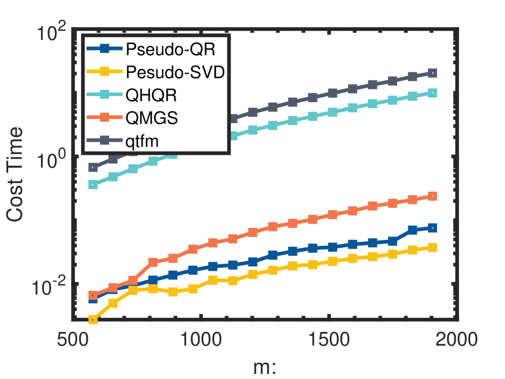
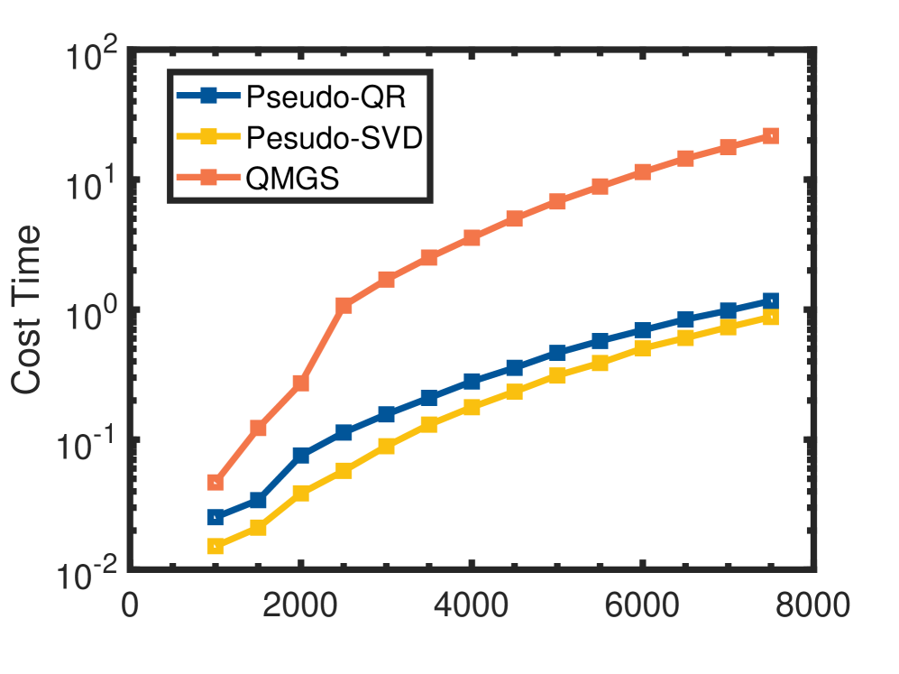
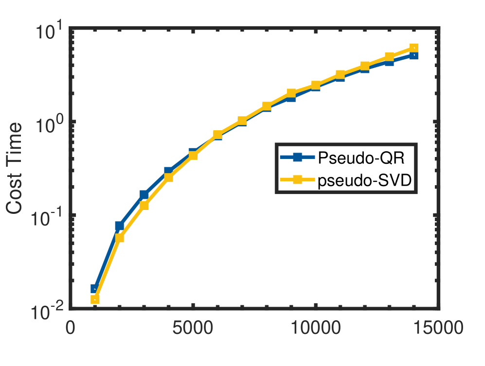
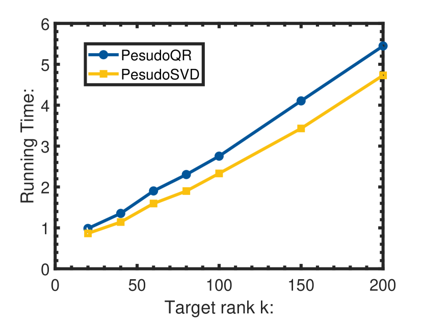
Subsequently, we will juxtapose these algorithms with other rangefinders, including the qr function in QTFM, the structure-preserving Quaternion Householder QR (QHQR) [19], and the structure-preserving modified Gram-Schmidt QR (QMGS) [2]. Figure 2(a) illustrates that our rangefinders exhibit significantly lower computational costs compared to qr in QTFM and the QHQR. The disparity in their time complexity can span two to three orders of magnitude, escalating with an increase in the size of the sketches from 600600600 to 200020002000. As the size continues to grow, Figure 2(b) demonstrates that our rangefinders outperform the QMGS algorithm markedly, while the qr function in QTFM and QHQR become prohibitively time-consuming. Finally, Figure 2(c) reveals that Pseudo-QR operates marginally faster than Pseudo-SVD when the data size exceeds 104superscript10410^{4}.

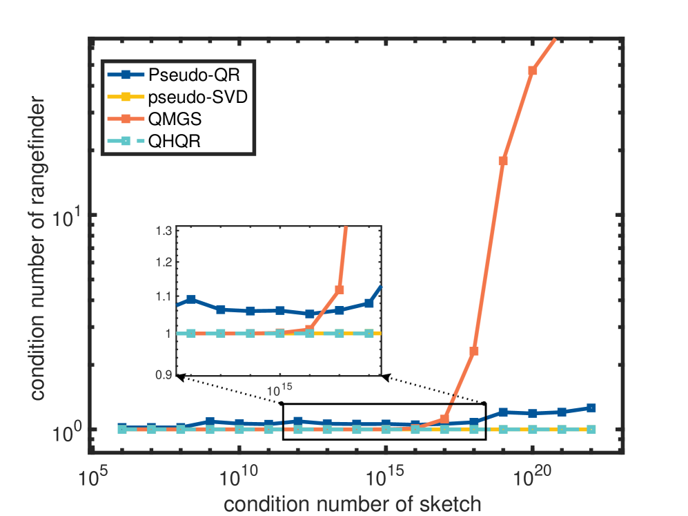
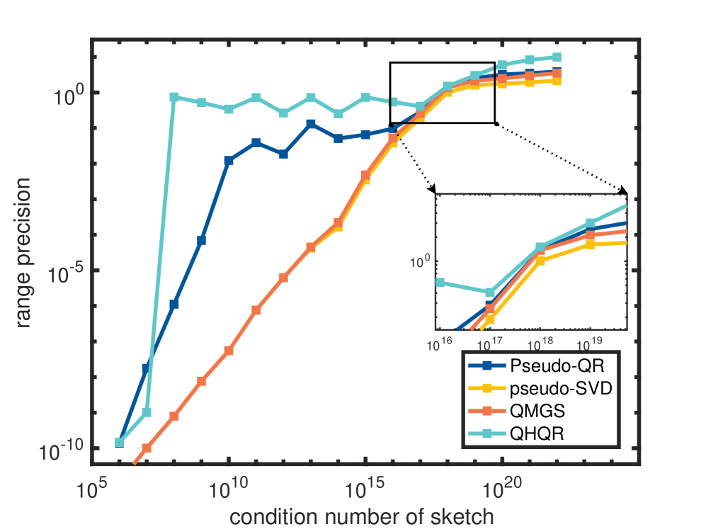
We then fixe the size of 𝐘𝐘\mathbf{Y} to be 1000×20010002001000\times 200 while vary κ(𝐘)𝜅𝐘\kappa(\mathbf{Y}) and compare their precision as illustrated in Fig. 3. In terms of the condition number of the rangefinder, all the rangefinders perform well when κ(𝐘)<1016𝜅𝐘superscript1016\kappa(\mathbf{Y})<10^{16}, and the orthonormal ones (Pseudo-SVD, QMGS, QHQR) keep their orthogonality. In terms of the range precision 𝐇𝐇𝐘𝐘Fsubscriptnormsuperscript𝐇𝐇superscript𝐘𝐘𝐹\parallel\mathbf{H}\mathbf{H}^{\dagger}-\mathbf{Y}\mathbf{Y}^{\dagger}\parallel_{F}, Pseudo-SVD and MGSQR outperform the competetors, while Pesudo-QR is still valuable when κ(𝐘)<108𝜅𝐘superscript108\kappa(\mathbf{Y})<10^{8}.

Refer to caption
(a) All rangefinders
Refer to caption
(b) QMGS, our rangefinders
Refer to caption
(c) our rangefidners
Figure 2: Running Time m=25n𝑚25𝑛m=25n, x-axis is m𝑚m and y-axis is running time with Logarithmic scale.
Refer to caption
(a) Condition Number
Refer to caption
(b) Range Precision
Figure 3: m=1000𝑚1000m=1000, n=200𝑛200n=200, condition number of sketch from 1e61𝑒61e6 to 1e221𝑒221e22.

4 One-Pass Algorithm

In this section, we consider the one-pass randomized algorithm proposed by Tropp et al. [41] with a range-preserving while possibly non-orthonormal rangefinder. The one-pass algorithm can reduce storage cost and ensure linear update of streaming data, where the latter can save multiplication flops during sketching [41, 42].

Our theoretical result shows that the accuracy loss of the truncation approximation is proportional to the condition number κ(𝐇)𝜅𝐇\kappa(\mathbf{H}). More detailed estimation with Gaussian and sub-Gaussian embeddings will be left to Sections 5 and 6.

4.1 The algorithm

For a given data matrix 𝐀m×n𝐀superscript𝑚𝑛\mathbf{A}\in\mathbb{Q}^{m\times n} and the target rank r𝑟r, the purpose is to find a rank-r𝑟r approximation. First draw two random quaternion 𝚿l×m𝚿superscript𝑙𝑚\boldsymbol{\boldsymbol{\Psi}}\in\mathbb{Q}^{l\times m} and 𝛀m×s𝛀superscript𝑚𝑠\boldsymbol{\Omega}\in\mathbb{Q}^{m\times s} independently where the sketch size satisfy: rslmin{m,n}𝑟𝑠𝑙𝑚𝑛r\leq s\leq l\leq\min\{m,n\}. Then main information can be captured by two sketches:

𝐘=𝐀𝛀s×mand𝐖=𝚿𝐀l×n,formulae-sequence𝐘𝐀𝛀superscript𝑠𝑚and𝐖𝚿𝐀superscript𝑙𝑛\displaystyle\mathbf{Y}=\mathbf{A}\boldsymbol{\Omega}\in\mathbb{Q}^{s\times m}\quad\text{and}\quad\mathbf{W}=\boldsymbol{\Psi}\mathbf{A}\in\mathbb{Q}^{l\times n}, (17)

where 𝐘𝐘\mathbf{Y} is used to generate the range 𝐇𝐇\mathbf{H} by using any range-preserving rangefinders such as pesudo-QR or pesudo-SVD.Then, a rank-s𝑠s QB approximation can be obtained by solving

𝐇𝐗=𝐇(𝚿𝐇)𝐖.𝐇𝐗𝐇superscript𝚿𝐇𝐖\displaystyle\mathbf{H}\mathbf{X}=\mathbf{H}\left(\boldsymbol{\Psi}\mathbf{H}\right)^{\dagger}\mathbf{W}. (18)

Finally, a truncated QSVD is applied to 𝐗𝐗\mathbf{X} to further obtain the final rank-r𝑟r approximation. In the recovery algorithm, only 𝐘𝐘\mathbf{Y}, 𝐖𝐖\mathbf{W}, and 𝚿𝚿\boldsymbol{\Psi} are required, which means that 𝐀𝐀\mathbf{A} is not exposed to the recovery process. The pseudocode is given in Algorithms 4 and 5.

Algorithm 4 QB Stage
1:Quaternion sketch 𝐘m×s,𝐖l×nformulae-sequence𝐘superscript𝑚𝑠𝐖superscript𝑙𝑛\mathbf{Y}\in\mathbb{Q}^{m\times s},\mathbf{W}\in\mathbb{Q}^{l\times n}, test matrices 𝚿l×m𝚿superscript𝑙𝑚\boldsymbol{\Psi}\in\mathbb{Q}^{l\times m},
2:Rank-s𝑠s approximation of the form 𝐀^=𝐇𝐗m×n^𝐀𝐇𝐗superscript𝑚𝑛\hat{\mathbf{A}}=\mathbf{H}\mathbf{X}\in\mathbb{Q}^{m\times n} with 𝐇m×s𝐇superscript𝑚𝑠\mathbf{H}\in\mathbb{Q}^{m\times s} and 𝐗s×n𝐗superscript𝑠𝑛\mathbf{X}\in\mathbb{Q}^{s\times n}
3:𝐇(𝐘)𝐇𝐘\mathbf{H}\leftarrow\mathcal{F}(\mathbf{Y}) \triangleright \mathcal{F} is a rangefinder map.
4:𝐗(𝚿𝐇)\𝐖𝐗\𝚿𝐇𝐖\mathbf{X}\leftarrow\left(\boldsymbol{\Psi}\mathbf{H}\right)\backslash\mathbf{W} \triangleright Solving overdetermined quaternion linear equations
5:return (𝐇,𝐗)𝐇𝐗\left(\mathbf{H},\mathbf{X}\right)
Algorithm 5 Truncation Stage
1:(𝐇,𝐗)𝐇𝐗(\mathbf{H},\mathbf{X}) from Algorithm 4
2:Rank-r𝑟r approximation 𝐀^=𝐔Σ𝐕^𝐀𝐔Σsuperscript𝐕\hat{\mathbf{A}}=\mathbf{U}\Sigma\mathbf{V}^{*} with 𝐔m×r𝐔superscript𝑚𝑟\mathbf{U}\in\mathbb{Q}^{m\times r}, orthonormal 𝐕n×r𝐕superscript𝑛𝑟\mathbf{V}\in\mathbb{Q}^{n\times r}, and real diagonal matrix Σr×rΣsuperscript𝑟𝑟\Sigma\in\mathbb{R}^{r\times r}.
3:(𝐔,Σ,𝐕)=QSVD(𝐗)𝐔Σ𝐕QSVD𝐗(\mathbf{U},\Sigma,\mathbf{V})={\rm QSVD}(\mathbf{X})
4:Σ=Σ(1:r,1:r)\Sigma=\Sigma(1:r,1:r), 𝐔=𝐔(:,1:r)\mathbf{U}=\mathbf{U}(:,1:r), 𝐕=𝐕(:,1:r)\mathbf{V}=\mathbf{V}(:,1:r)
5:𝐔=𝐇𝐔𝐔𝐇𝐔\mathbf{U}=\mathbf{H}\mathbf{U}
6:return (𝐔,Σ,𝐕)𝐔Σ𝐕\left(\mathbf{U},\Sigma,\mathbf{V}\right)
Remark 4.1.

To solve (𝚿𝐇)\𝐖\𝚿𝐇𝐖\left(\boldsymbol{\Psi}\mathbf{H}\right)\backslash\mathbf{W}, one can use Algorithm 1 in the complex arithmetic. QSVD in the truncation stage can be any quaternion SVD algorithms [26, 37, 16, 25] or directly computing the SVD of χ𝐗subscript𝜒𝐗{\chi}_{\mathbf{X}}.

Remark 4.2.

Even though 𝐇𝐇\mathbf{H} may be non-orthonormal, empirically, we find that a truncation stage is still helpful in improving the recovery accuracy than only doing a QB approximation. This is the same as the orthonormal case [41, 14, 27].

4.2 Deterministic error

This subsection is only concerned with the deterministic error without assuming the distribution of the test matrices at first. More detailed probabilistic bounds will be given in Sections 5 and 6 when a randomized embedding is selected. The following basic requirements on the rangefinder 𝐇𝐇\mathbf{H} and the sketch size are made througout this subsection:

(𝐇)𝐇\displaystyle{\mathcal{R}}(\mathbf{H}) =(𝐘),and𝐇hasfullcolumnrank;absent𝐘and𝐇hasfullcolumnrank\displaystyle={\mathcal{R}}(\mathbf{Y}),~{}{\rm and}~{}\mathbf{H}~{}{\rm has~{}full~{}column~{}rank}; (19)
rs𝑟𝑠\displaystyle r\leq s lmin{m,n}.absent𝑙𝑚𝑛\displaystyle\leq l\leq\min\{m,n\}. (20)

To analyze the approximation error with a non-orthonormal 𝐇𝐇\mathbf{H}, the idea is to use QB decomposition as a bridge such that existing error analysis can be applied. One can represent 𝐇𝐇\mathbf{H} as:

𝐇=𝐐𝐁,𝐐m×s,𝐐𝐐=Is.formulae-sequence𝐇𝐐𝐁formulae-sequence𝐐superscript𝑚𝑠superscript𝐐𝐐subscript𝐼𝑠\displaystyle\mathbf{H}=\mathbf{Q}\mathbf{B},~{}\mathbf{Q}\in\mathbb{Q}^{m\times s},~{}\mathbf{Q}^{*}\mathbf{Q}=I_{s}. (21)

Under (19), (𝐐)=(𝐇)=(𝐘)𝐐𝐇𝐘{\mathcal{R}}(\mathbf{Q})={\mathcal{R}}(\mathbf{H})={\mathcal{R}}(\mathbf{Y}) and 𝐁s×s𝐁superscript𝑠𝑠\mathbf{B}\in\mathbb{Q}^{s\times s} is invertible. Here (21) can be thin QR, compact QSVD, or polar decomposition.

We introduce notations used in this subsection. Define the partially orthonormal matrix 𝐐m×(ms)subscript𝐐bottomsuperscript𝑚𝑚𝑠\mathbf{Q}_{\bot}\in\mathbb{Q}^{m\times(m-s)} with 𝐐𝐐:=Im𝐐𝐐\mathbf{Q}_{\bot}\mathbf{Q}_{\bot}^{*}:=I_{m}-\mathbf{Q}\mathbf{Q}* such that (𝐐)(𝐐)perpendicular-to𝐐subscript𝐐bottom{\mathcal{R}}(\mathbf{Q})\perp{\mathcal{R}}(\mathbf{Q}_{\bot}). Then we define submatrices:

𝚿1=𝚿𝐐l×(ms),𝚿2=𝚿𝐐l×s.formulae-sequencesubscript𝚿1𝚿subscript𝐐bottomsuperscript𝑙𝑚𝑠subscript𝚿2𝚿𝐐superscript𝑙𝑠\displaystyle\boldsymbol{\Psi}_{1}=\boldsymbol{\Psi}\mathbf{Q}_{\bot}\in\mathbb{Q}^{l\times\left(m-s\right)},\quad\boldsymbol{\Psi}_{2}=\boldsymbol{\Psi}\mathbf{Q}\in\mathbb{Q}^{l\times s}. (22)

Let the QSVD of 𝐀m×n𝐀superscript𝑚𝑛\mathbf{A}\in\mathbb{Q}^{m\times n} be

𝐀=𝐔Σ𝐕=[𝐔1𝐔2][Σ100Σ2][𝐕1𝐕2],Σ1r×r,𝐔1m×r,𝐕1n×r;formulae-sequence𝐀𝐔Σsuperscript𝐕matrixsubscript𝐔1subscript𝐔2delimited-[]subscriptΣ100subscriptΣ2delimited-[]superscriptsubscript𝐕1superscriptsubscript𝐕2formulae-sequencesubscriptΣ1superscript𝑟𝑟formulae-sequencesubscript𝐔1superscript𝑚𝑟subscript𝐕1superscript𝑛𝑟\displaystyle\small\mathbf{A}=\mathbf{U}\Sigma\mathbf{V}^{*}=\begin{bmatrix}\mathbf{U}_{1}&\mathbf{U}_{2}\end{bmatrix}\left[\begin{array}[]{cc}\Sigma_{1}&0\\ 0&\Sigma_{2}\end{array}\right]\left[\begin{array}[]{c}\mathbf{V}_{1}^{*}\\ \mathbf{V}_{2}^{*}\end{array}\right],~{}\Sigma_{1}\in\mathbb{R}^{r\times r},~{}\mathbf{U}_{1}\in\mathbb{Q}^{m\times r},~{}\mathbf{V}_{1}\in\mathbb{Q}^{n\times r}; (27)

and define:

𝛀1=𝐕1𝛀r×s,subscript𝛀1superscriptsubscript𝐕1𝛀superscript𝑟𝑠\displaystyle\boldsymbol{\Omega}_{1}=\mathbf{V}_{1}^{*}\boldsymbol{\Omega}\in\mathbb{Q}^{r\times s}, 𝛀2=𝐕2𝛀(nr)×s.subscript𝛀2superscriptsubscript𝐕2𝛀superscript𝑛𝑟𝑠\displaystyle\quad\boldsymbol{\Omega}_{2}=\mathbf{V}_{2}^{*}\boldsymbol{\Omega}\in\mathbb{Q}^{\left(n-r\right)\times s}. (28)

The error of Algorithm 4, which is independent of κ(𝐇)𝜅𝐇\kappa(\mathbf{H}), is provided.

Theorem 4.1 (QB error).

Let (𝐇,𝐗)𝐇𝐗(\mathbf{H},\mathbf{X}) be generated by Algorithm 4 and (19) holds. With notations in (22) and (28), if 𝛀1superscriptsubscript𝛀1\boldsymbol{\Omega}_{1}^{*} and 𝚿2subscript𝚿2\boldsymbol{\Psi}_{2} have full column rank, we have the following error estimation, where “a𝑎a{F,2}absent𝐹2\in\{F,2\}:

𝐇𝐗𝐀asubscriptnorm𝐇𝐗𝐀𝑎\displaystyle\|\mathbf{H}\mathbf{X}-\mathbf{A}\|_{a} 𝐀𝐐𝐐𝐀a+𝚿2𝚿1(𝐐𝐀)aabsentsubscriptnorm𝐀superscript𝐐𝐐𝐀𝑎subscriptnormsuperscriptsubscript𝚿2subscript𝚿1superscriptsubscript𝐐bottom𝐀𝑎\displaystyle\leq\parallel\mathbf{A}-\mathbf{Q}\mathbf{Q}^{*}\mathbf{A}\parallel_{a}+\parallel\boldsymbol{\Psi}_{2}^{\dagger}\boldsymbol{\Psi}_{1}(\mathbf{Q}_{\bot}^{*}\mathbf{A})\parallel_{a} (29)
(1+𝚿22𝚿12)(1+𝛀22𝛀12)Σ2a;absent1subscriptnormsuperscriptsubscript𝚿22subscriptnormsubscript𝚿121subscriptnormsubscript𝛀22subscriptnormsuperscriptsubscript𝛀12subscriptnormsubscriptΣ2𝑎\displaystyle\leq\left(1+\parallel\boldsymbol{\Psi}_{2}^{\dagger}\parallel_{2}\parallel\boldsymbol{\Psi}_{1}\parallel_{2}\right)\left(1+\parallel\boldsymbol{\Omega}_{2}\parallel_{2}\parallel\boldsymbol{\Omega}_{1}^{\dagger}\parallel_{2}\right)\|\Sigma_{2}\|_{a}; (30)

in particular,

𝐀(𝚿𝐐)𝚿𝐀F2=𝐀𝐐𝐐𝐀F2+𝚿2𝚿1(𝐐𝐀)F2.superscriptsubscriptnorm𝐀superscript𝚿𝐐𝚿𝐀𝐹2superscriptsubscriptnorm𝐀superscript𝐐𝐐𝐀𝐹2superscriptsubscriptnormsuperscriptsubscript𝚿2subscript𝚿1superscriptsubscript𝐐bottom𝐀𝐹2\displaystyle\parallel\mathbf{A}-\left(\boldsymbol{\Psi}\mathbf{Q}\right)^{\dagger}\boldsymbol{\Psi}\mathbf{A}\parallel_{F}^{2}=\|\mathbf{A}-\mathbf{Q}\mathbf{Q}^{*}\mathbf{A}\|_{F}^{2}+\|\boldsymbol{\Psi}_{2}^{\dagger}\boldsymbol{\Psi}_{1}\left(\mathbf{Q}_{\bot}^{*}\mathbf{A}\right)\|_{F}^{2}. (31)

Recall that 𝐗=(𝚿𝐇)𝚿𝐀𝐗superscript𝚿𝐇𝚿𝐀\mathbf{X}=\left(\boldsymbol{\Psi}\mathbf{H}\right)^{\dagger}\boldsymbol{\Psi}\mathbf{A} in Algorithm 4. Denote 𝐗rsubscript𝐗𝑟\lfloor\mathbf{X}\rfloor_{r} as the best rank-r𝑟r approximation of 𝐗𝐗\mathbf{X}. Analygous to the real/complex counterpart, 𝐗rsubscript𝐗𝑟\lfloor\mathbf{X}\rfloor_{r} is also given by the rank-r𝑟r turncated QSVD [22]. The truncation error is estimated in the following theorem:

Theorem 4.2 (Truncation error).

Let 𝐇𝐇\mathbf{H}, 𝐗𝐗\mathbf{X} be generated by Algorithm 4 with (19) hold, and 𝐗rsubscript𝐗𝑟\lfloor\mathbf{X}\rfloor_{r} be truncated by Algorithm 5. Then

𝐇𝐗r𝐇𝐗aκ(𝐇)(𝐀𝐇𝐗a+τr(𝐀)).subscriptnorm𝐇subscript𝐗𝑟𝐇𝐗𝑎𝜅𝐇subscriptnorm𝐀𝐇𝐗𝑎subscript𝜏𝑟𝐀\displaystyle\parallel\mathbf{H}\lfloor\mathbf{X}\rfloor_{r}-\mathbf{H}\mathbf{X}\parallel_{a}\leq\kappa(\mathbf{H})\left(\parallel\mathbf{A}-\mathbf{H}\mathbf{X}\parallel_{a}+\tau_{r}(\mathbf{A})\right). (32)

To make the proof of Theorem 4.1 clear, we devide it in a series of lemmas.

Lemma 4.1.

Let 𝐀m×n𝐀superscript𝑚𝑛\mathbf{A}\in\mathbb{Q}^{m\times n} and 𝐁n×p𝐁superscript𝑛𝑝\mathbf{B}\in\mathbb{Q}^{n\times p}; then (𝐀𝐁)𝐁𝐀superscript𝐀𝐁superscript𝐁superscript𝐀(\mathbf{A}\mathbf{B})^{\dagger}\neq\mathbf{B}^{\dagger}\mathbf{A}^{\dagger} in general. However, we have the following sufficient conditions for (𝐀𝐁)=𝐁𝐀superscript𝐀𝐁superscript𝐁superscript𝐀(\mathbf{A}\mathbf{B})^{\dagger}=\mathbf{B}^{\dagger}\mathbf{A}^{\dagger}:

  1. 1.

    𝐀𝐀\mathbf{A} has orthonormal columns (𝐀𝐀=𝐀𝐀=Isuperscript𝐀𝐀superscript𝐀𝐀𝐼\mathbf{A}^{*}\mathbf{A}=\mathbf{A}^{\dagger}\mathbf{A}=I) or

  2. 2.

    𝐁𝐁\mathbf{B} has orthonormal rows (𝐁𝐁=𝐁𝐁=Isuperscript𝐁𝐁superscript𝐁𝐁𝐼\mathbf{B}\mathbf{B}^{*}=\mathbf{B}\mathbf{B}^{\dagger}=I) or

  3. 3.

    𝐀𝐀\mathbf{A} has full column rank (𝐀𝐀=Isuperscript𝐀𝐀𝐼\mathbf{A}^{\dagger}\mathbf{A}=I) and 𝐁𝐁\mathbf{B} has full row rank (𝐁𝐁=Isuperscript𝐁𝐁𝐼\mathbf{B}\mathbf{B}^{\dagger}=I) or

  4. 4.

    𝐁=𝐀𝐁superscript𝐀\mathbf{B}=\mathbf{A}^{*} or

  5. 5.

    𝐁=𝐀𝐁superscript𝐀\mathbf{B}=\mathbf{A}^{\dagger}.

Proof.

By Lemma 2.2, it suffices to prove (χ𝐀χ𝐁)=χ𝐁χ𝐀superscriptsubscript𝜒𝐀subscript𝜒𝐁superscriptsubscript𝜒𝐁superscriptsubscript𝜒𝐀\left(\chi_{\mathbf{A}}\chi_{\mathbf{B}}\right)^{\dagger}=\chi_{\mathbf{B}}^{\dagger}\chi_{\mathbf{A}}^{\dagger}. For two complex matrices E𝐸E and F𝐹F, [13] proved that (EF)=FEsuperscript𝐸𝐹superscript𝐹superscript𝐸(EF)^{\dagger}=F^{\dagger}E^{\dagger} holds if and only if:

EEFFEEFF=FFEE.superscript𝐸𝐸𝐹superscript𝐹superscript𝐸𝐸𝐹superscript𝐹𝐹superscript𝐹superscript𝐸𝐸\displaystyle E^{\dagger}EFF^{*}E^{*}EFF^{\dagger}=FF^{*}E^{*}E. (33)

Let E=χ𝐀𝐸subscript𝜒𝐀E={\chi}_{\mathbf{A}}, F=χ𝐁𝐹subscript𝜒𝐁F=\chi_{\mathbf{B}}. Using the properties of generalized inverse and complex representation of quaternion matrices, one can check that each condition in this lemma can make (33) hold.∎

Lemma 4.2.

Let 𝐇m×s(ms)𝐇superscript𝑚𝑠𝑚𝑠\mathbf{H}\in\mathbb{Q}^{m\times s}~{}(m\geq s) have full column rank, 𝐐m×s𝐐superscript𝑚𝑠\mathbf{Q}\in\mathbb{Q}^{m\times s} is given by (21), and 𝚿𝚿\boldsymbol{\Psi} is an arbitrary l×m(slm)𝑙𝑚𝑠𝑙𝑚l\times m~{}(s\leq l\leq m) quaternion matrix with full row rank. Then we have:

𝐇𝐗=𝐇(𝚿𝐇)𝚿𝐀𝐇𝐗𝐇superscript𝚿𝐇𝚿𝐀\displaystyle\mathbf{H}\mathbf{X}=\mathbf{H}\left(\boldsymbol{\Psi}\mathbf{H}\right)^{\dagger}\boldsymbol{\Psi}\mathbf{A} =𝐐(𝚿𝐐)𝚿𝐀.absent𝐐superscript𝚿𝐐𝚿𝐀\displaystyle=\mathbf{Q}(\boldsymbol{\Psi}\mathbf{Q})^{\dagger}\boldsymbol{\Psi}\mathbf{A}. (34)
Proof.

Let 𝐇=𝐐𝐁𝐇𝐐𝐁\mathbf{H}=\mathbf{Q}\mathbf{B} where 𝐁s×s𝐁superscript𝑠𝑠\mathbf{B}\in\mathbb{Q}^{s\times s} is invertible. Then

𝐇(𝚿𝐇)𝚿𝐀𝐇superscript𝚿𝐇𝚿𝐀\displaystyle\mathbf{H}\left(\boldsymbol{\Psi}\mathbf{H}\right)^{\dagger}\boldsymbol{\Psi}\mathbf{A} =𝐐𝐁(𝚿𝐐𝐁)𝚿𝐀absent𝐐𝐁superscript𝚿𝐐𝐁𝚿𝐀\displaystyle=\mathbf{Q}\mathbf{B}(\boldsymbol{\Psi}\mathbf{Q}\mathbf{B})^{\dagger}\boldsymbol{\Psi}\mathbf{A}
(Lemma 4.1, point 3) =𝐐𝐁𝐁1(𝚿𝐐)𝚿𝐀absentsuperscript𝐐𝐁𝐁1superscript𝚿𝐐𝚿𝐀\displaystyle=\mathbf{Q}\mathbf{B}\mathbf{B}^{-1}(\boldsymbol{\Psi}\mathbf{Q})^{\dagger}\boldsymbol{\Psi}\mathbf{A}
=𝐐(𝚿𝐐)𝚿𝐀.absent𝐐superscript𝚿𝐐𝚿𝐀\displaystyle=\mathbf{Q}(\boldsymbol{\Psi}\mathbf{Q})^{\dagger}\boldsymbol{\Psi}\mathbf{A}.

The second identity is from Lemma 4.1 because 𝚿𝐐l×s(ls)𝚿𝐐superscript𝑙𝑠𝑙𝑠\boldsymbol{\Psi}\mathbf{Q}\in\mathbb{Q}^{l\times s}(l\geq s) has full column rank (𝚿superscript𝚿\boldsymbol{\Psi}^{*} and 𝐐𝐐\mathbf{Q} are both of full column rank) and 𝐁𝐁\mathbf{B} is invertible. ∎

The following lemma is a trivial quaternion version of [41, Lemma A.4].

Lemma 4.3.

Assume that 𝚿2subscript𝚿2\boldsymbol{\Psi}_{2} has full column rank; then

(𝚿𝐐)𝚿𝐀𝐐𝐀=𝚿2𝚿1(𝐐𝐀).superscript𝚿𝐐𝚿𝐀superscript𝐐𝐀superscriptsubscript𝚿2subscript𝚿1superscriptsubscript𝐐bottom𝐀\displaystyle\left(\boldsymbol{\Psi}\mathbf{Q}\right)^{\dagger}\boldsymbol{\Psi}\mathbf{A}-\mathbf{Q}^{*}\mathbf{A}=\boldsymbol{\Psi}_{2}^{\dagger}\boldsymbol{\Psi}_{1}\left(\mathbf{Q}_{\bot}^{*}\mathbf{A}\right).

The follow lemma comes from [27, Section 4.3]; see also [14, Theorem 9.1].

Lemma 4.4 (deterministic error bound).

With the notations in Algorithm 4 and in (28), and 𝐐𝐐\mathbf{Q} is as in Lemma 4.2,

𝐀𝐐𝐐𝐀a2superscriptsubscriptnorm𝐀superscript𝐐𝐐𝐀𝑎2\displaystyle\parallel\mathbf{A}-\mathbf{Q}\mathbf{Q}^{*}\mathbf{A}\parallel_{a}^{2} Σ2a2+Σ2𝛀2(𝛀1)a2absentsuperscriptsubscriptnormsubscriptΣ2𝑎2superscriptsubscriptnormsubscriptΣ2superscriptsubscript𝛀2superscriptsuperscriptsubscript𝛀1𝑎2\displaystyle\leq\parallel\Sigma_{2}\parallel_{a}^{2}+\parallel\Sigma_{2}\boldsymbol{\Omega}_{2}^{*}\left(\boldsymbol{\Omega}_{1}^{*}\right)^{\dagger}\parallel_{a}^{2}
(Σ2a+Σ2𝛀2(𝛀1)a)2.absentsuperscriptsubscriptnormsubscriptΣ2𝑎subscriptnormsubscriptΣ2superscriptsubscript𝛀2superscriptsuperscriptsubscript𝛀1𝑎2\displaystyle\leq\left(\parallel\Sigma_{2}\parallel_{a}+\parallel\Sigma_{2}\boldsymbol{\Omega}_{2}^{*}\left(\boldsymbol{\Omega}_{1}^{*}\right)^{\dagger}\parallel_{a}\right)^{2}.

Now we prove Theorem 4.1. Note that (𝐗)=(𝐗)superscriptsuperscript𝐗superscriptsuperscript𝐗\left(\mathbf{X}^{\dagger}\right)^{*}=\left(\mathbf{X}^{*}\right)^{\dagger} will be frequently used in the proof.

Proof of Theorem 4.1.

By Lemma 4.2, it holds that

𝐀𝐇𝐗a=𝐀𝐇(𝚿𝐇)𝚿𝐀a=𝐀𝐐(𝚿𝐐)𝚿𝐀a.subscriptnorm𝐀𝐇𝐗𝑎subscriptnorm𝐀𝐇superscript𝚿𝐇𝚿𝐀𝑎subscriptnorm𝐀𝐐superscript𝚿𝐐𝚿𝐀𝑎\displaystyle\parallel\mathbf{A}-\mathbf{H}\mathbf{X}\parallel_{a}=\parallel\mathbf{A}-\mathbf{H}\left(\boldsymbol{\Psi}\mathbf{H}\right)^{\dagger}\boldsymbol{\Psi}\mathbf{A}\parallel_{a}=\parallel\mathbf{A}-\mathbf{Q}(\boldsymbol{\Psi}\mathbf{Q})^{\dagger}\boldsymbol{\Psi}\mathbf{A}\parallel_{a}. (35)

Thus, it suffices to evaluate the right part of (35). Then,

𝐀𝐐(𝚿𝐐)𝚿𝐀asubscriptnorm𝐀𝐐superscript𝚿𝐐𝚿𝐀𝑎\displaystyle\|\mathbf{A}-\mathbf{Q}(\boldsymbol{\Psi}\mathbf{Q})^{\dagger}\boldsymbol{\Psi}\mathbf{A}\|_{a} 𝐀𝐐𝐐𝐀a+𝐐(𝚿𝐐)𝚿𝐀𝐐𝐐𝐀aabsentsubscriptnorm𝐀superscript𝐐𝐐𝐀𝑎subscriptnorm𝐐superscript𝚿𝐐𝚿𝐀superscript𝐐𝐐𝐀𝑎\displaystyle\leq\|\mathbf{A}-\mathbf{Q}\mathbf{Q}^{*}\mathbf{A}\|_{a}+\|\mathbf{Q}(\boldsymbol{\Psi}\mathbf{Q})^{\dagger}\boldsymbol{\Psi}\mathbf{A}-\mathbf{Q}\mathbf{Q}^{*}\mathbf{A}\|_{a}
=𝐀𝐐𝐐𝐀a+𝚿2𝚿1(𝐐𝐀)a,absentsubscriptnorm𝐀superscript𝐐𝐐𝐀𝑎subscriptnormsuperscriptsubscript𝚿2subscript𝚿1superscriptsubscript𝐐bottom𝐀𝑎\displaystyle=\|\mathbf{A}-\mathbf{Q}\mathbf{Q}^{*}\mathbf{A}\|_{a}+\|\boldsymbol{\Psi}_{2}^{\dagger}\boldsymbol{\Psi}_{1}\left(\mathbf{Q}_{\bot}^{*}\mathbf{A}\right)\|_{a},

where the equality uses that both Frobenius and spectral norm are unitary invariant and by Lemma 4.3. Note that

𝚿2𝚿1(𝐐𝐀)a𝚿22𝚿12𝐐𝐀asubscriptnormsuperscriptsubscript𝚿2subscript𝚿1superscriptsubscript𝐐bottom𝐀𝑎subscriptnormsuperscriptsubscript𝚿22subscriptnormsubscript𝚿12subscriptnormsuperscriptsubscript𝐐bottom𝐀𝑎\displaystyle\|\boldsymbol{\Psi}_{2}^{\dagger}\boldsymbol{\Psi}_{1}\left(\mathbf{Q}_{\bot}^{*}\mathbf{A}\right)\|_{a}\leq\parallel\boldsymbol{\Psi}_{2}^{\dagger}\parallel_{2}\parallel\boldsymbol{\Psi}_{1}\parallel_{2}\|\mathbf{Q}_{\bot}^{*}\mathbf{A}\|_{a} (36)

and

𝐐𝐀a=𝐐𝐐𝐀a=𝐀𝐐𝐐𝐀a;subscriptnormsuperscriptsubscript𝐐bottom𝐀𝑎subscriptnormsubscript𝐐bottomsuperscriptsubscript𝐐bottom𝐀𝑎subscriptnorm𝐀superscript𝐐𝐐𝐀𝑎\displaystyle\|\mathbf{Q}_{\bot}^{*}\mathbf{A}\|_{a}=\|\mathbf{Q}_{\bot}\mathbf{Q}_{\bot}^{*}\mathbf{A}\|_{a}=\|\mathbf{A}-\mathbf{Q}\mathbf{Q}^{*}\mathbf{A}\|_{a};

it follows from Lemma 4.4 that

𝐀𝐐𝐐𝐀a(1+(𝛀1)2𝛀22)Σ2a.subscriptnorm𝐀superscript𝐐𝐐𝐀𝑎1subscriptnormsuperscriptsuperscriptsubscript𝛀12subscriptnormsuperscriptsubscript𝛀22subscriptnormsubscriptΣ2𝑎\displaystyle\|\mathbf{A}-\mathbf{Q}\mathbf{Q}^{*}\mathbf{A}\|_{a}\leq\left(1+\parallel\left(\boldsymbol{\Omega}_{1}^{*}\right)^{\dagger}\parallel_{2}\parallel\boldsymbol{\Omega}_{2}^{*}\parallel_{2}\right)\parallel\Sigma_{2}\parallel_{a}.

In particular, using 𝚿2𝚿1(𝐐𝐀)=𝐐(𝚿𝐐)𝚿𝐀𝐐𝐐𝐀superscriptsubscript𝚿2subscript𝚿1superscriptsubscript𝐐bottom𝐀𝐐superscript𝚿𝐐𝚿𝐀superscript𝐐𝐐𝐀\boldsymbol{\Psi}_{2}^{\dagger}\boldsymbol{\Psi}_{1}\left(\mathbf{Q}_{\bot}^{*}\mathbf{A}\right)=\mathbf{Q}(\boldsymbol{\Psi}\mathbf{Q})^{\dagger}\boldsymbol{\Psi}\mathbf{A}-\mathbf{Q}\mathbf{Q}^{*}\mathbf{A} and Pythagorean identity,

𝐀𝐐(𝚿𝐐)𝚿𝐀F2superscriptsubscriptnorm𝐀𝐐superscript𝚿𝐐𝚿𝐀𝐹2\displaystyle\parallel\mathbf{A}-\mathbf{Q}(\boldsymbol{\Psi}\mathbf{Q})^{\dagger}\boldsymbol{\Psi}\mathbf{A}\parallel_{F}^{2} =𝐀𝐐𝐐𝐀+𝐐𝐐𝐀𝐐(𝚿𝐐)𝚿𝐀F2absentsuperscriptsubscriptnorm𝐀superscript𝐐𝐐𝐀superscript𝐐𝐐𝐀𝐐superscript𝚿𝐐𝚿𝐀𝐹2\displaystyle=\parallel\mathbf{A}-\mathbf{Q}\mathbf{Q}^{*}\mathbf{A}+\mathbf{Q}\mathbf{Q}^{*}\mathbf{A}-\mathbf{Q}(\boldsymbol{\Psi}\mathbf{Q})^{\dagger}\boldsymbol{\Psi}\mathbf{A}\parallel_{F}^{2}
=𝐀𝐐𝐐𝐀F2+𝚿2𝚿1(𝐐𝐀)F2.absentsuperscriptsubscriptnorm𝐀superscript𝐐𝐐𝐀𝐹2superscriptsubscriptnormsuperscriptsubscript𝚿2subscript𝚿1superscriptsubscript𝐐bottom𝐀𝐹2\displaystyle=\|\mathbf{A}-\mathbf{Q}\mathbf{Q}^{*}\mathbf{A}\|_{F}^{2}+\|\boldsymbol{\Psi}_{2}^{\dagger}\boldsymbol{\Psi}_{1}\left(\mathbf{Q}_{\bot}^{*}\mathbf{A}\right)\|_{F}^{2}.

Proof of Theorem 4.2.

Let 𝐇=𝐐𝐁𝐇𝐐𝐁\mathbf{H}=\mathbf{Q}\mathbf{B} as (21) where 𝐐𝐐\mathbf{Q} is partially orthonormal and 𝐁𝐁\mathbf{B} is invertible. Then 𝐗=(𝚿𝐇)𝚿𝐀=(𝚿𝐐𝐁)𝚿𝐀=𝐁1(𝚿𝐐)𝚿𝐀𝐗superscript𝚿𝐇𝚿𝐀superscript𝚿𝐐𝐁𝚿𝐀superscript𝐁1superscript𝚿𝐐𝚿𝐀\mathbf{X}=\left(\boldsymbol{\Psi}\mathbf{H}\right)^{\dagger}\boldsymbol{\Psi}\mathbf{A}=\left(\boldsymbol{\Psi}\mathbf{Q}\mathbf{B}\right)^{\dagger}\boldsymbol{\Psi}\mathbf{A}=\mathbf{B}^{-1}\left(\boldsymbol{\Psi}\mathbf{Q}\right)^{\dagger}\boldsymbol{\Psi}\mathbf{A}, where the last equality follows from the proof of Lemma 4.2 and that a random fat 𝚿l×m𝚿superscript𝑙𝑚\boldsymbol{\Psi}\in\mathbb{Q}^{l\times m} drawn from continuous distribution has full row rank genericly. Denote 𝐀in:=𝐐(𝚿𝐐)𝚿𝐀assignsubscript𝐀𝑖𝑛𝐐superscript𝚿𝐐𝚿𝐀\mathbf{A}_{in}:=\mathbf{Q}(\boldsymbol{\Psi}\mathbf{Q})^{\dagger}\boldsymbol{\Psi}\mathbf{A}. We have:

𝐇𝐗𝐇𝐗rasubscriptnorm𝐇𝐗𝐇subscript𝐗𝑟𝑎\displaystyle\parallel\mathbf{H}\mathbf{X}-\mathbf{H}\lfloor\mathbf{X}\rfloor_{r}\parallel_{a} 𝐇2𝐗𝐗raabsentsubscriptnorm𝐇2subscriptnorm𝐗subscript𝐗𝑟𝑎\displaystyle\leq\parallel\mathbf{H}\parallel_{2}\parallel\mathbf{X}-\lfloor\mathbf{X}\rfloor_{r}\parallel_{a}
=𝐇2𝐁1(𝚿𝐐)𝚿𝐀𝐁1(𝚿𝐐)𝚿𝐀raabsentsubscriptnorm𝐇2subscriptnormsuperscript𝐁1superscript𝚿𝐐𝚿𝐀subscriptsuperscript𝐁1superscript𝚿𝐐𝚿𝐀𝑟𝑎\displaystyle=\parallel\mathbf{H}\parallel_{2}\parallel\mathbf{B}^{-1}(\boldsymbol{\Psi}\mathbf{Q})^{\dagger}\boldsymbol{\Psi}\mathbf{A}-\lfloor\mathbf{B}^{-1}(\boldsymbol{\Psi}\mathbf{Q})^{\dagger}\boldsymbol{\Psi}\mathbf{A}\rfloor_{r}\parallel_{a}
𝐇2𝐁1(𝚿𝐐)𝚿𝐀𝐁1(𝚿𝐐)𝚿𝐀raabsentsubscriptnorm𝐇2subscriptnormsuperscript𝐁1superscript𝚿𝐐𝚿𝐀superscript𝐁1subscriptsuperscript𝚿𝐐𝚿𝐀𝑟𝑎\displaystyle\leq\parallel\mathbf{H}\parallel_{2}\parallel\mathbf{B}^{-1}(\boldsymbol{\Psi}\mathbf{Q})^{\dagger}\boldsymbol{\Psi}\mathbf{A}-\mathbf{B}^{-1}\lfloor(\boldsymbol{\Psi}\mathbf{Q})^{\dagger}\boldsymbol{\Psi}\mathbf{A}\rfloor_{r}\parallel_{a}
𝐇2𝐁12(𝚿𝐐)𝚿𝐀(𝚿𝐐)𝚿𝐀raabsentsubscriptnorm𝐇2subscriptnormsuperscript𝐁12subscriptnormsuperscript𝚿𝐐𝚿𝐀subscriptsuperscript𝚿𝐐𝚿𝐀𝑟𝑎\displaystyle\leq\parallel\mathbf{H}\parallel_{2}\parallel\mathbf{B}^{-1}\parallel_{2}\cdot\parallel(\boldsymbol{\Psi}\mathbf{Q})^{\dagger}\boldsymbol{\Psi}\mathbf{A}-\lfloor(\boldsymbol{\Psi}\mathbf{Q})^{\dagger}\boldsymbol{\Psi}\mathbf{A}\rfloor_{r}\parallel_{a}
([41], 𝐐(𝚿𝐐)𝚿𝐀r=𝐀in)\mathbf{Q}\lfloor(\boldsymbol{\Psi}\mathbf{Q})^{\dagger}\boldsymbol{\Psi}\mathbf{A}\rfloor_{r}=\mathbf{A}_{in}) =κ(𝐇)𝐀in𝐀inraκ(𝐇)𝐀in𝐀raabsent𝜅𝐇subscriptnormsubscript𝐀𝑖𝑛subscriptsubscript𝐀𝑖𝑛𝑟𝑎𝜅𝐇subscriptnormsubscript𝐀𝑖𝑛subscript𝐀𝑟𝑎\displaystyle=\kappa(\mathbf{H})\parallel\mathbf{A}_{in}-\lfloor\mathbf{A}_{in}\rfloor_{r}\parallel_{a}~{}\leq\kappa(\mathbf{H})\parallel\mathbf{A}_{in}-\lfloor\mathbf{A}\rfloor_{r}\parallel_{a}
κ(𝐇)(𝐀in𝐀a+𝐀𝐀ra)absent𝜅𝐇subscriptnormsubscript𝐀𝑖𝑛𝐀𝑎subscriptnorm𝐀subscript𝐀𝑟𝑎\displaystyle\leq\kappa(\mathbf{H})(\parallel\mathbf{A}_{in}-\mathbf{A}\parallel_{a}+\parallel\mathbf{A}-\lfloor\mathbf{A}\rfloor_{r}\parallel_{a})
=κ(𝐇)(𝐀𝐇𝐗a+τr(𝐀)),absent𝜅𝐇subscriptnorm𝐀𝐇𝐗𝑎subscript𝜏𝑟𝐀\displaystyle=\kappa(\mathbf{H})\left(\parallel\mathbf{A}-\mathbf{H}\mathbf{X}\parallel_{a}+\tau_{r}(\mathbf{A})\right),

where the second inequality is because that 𝐁1(𝚿𝐐)𝚿𝐀rsuperscript𝐁1subscriptsuperscript𝚿𝐐𝚿𝐀𝑟\mathbf{B}^{-1}\lfloor(\boldsymbol{\Psi}\mathbf{Q})^{\dagger}\boldsymbol{\Psi}\mathbf{A}\rfloor_{r} has rank at most r𝑟r, which is no closer than 𝐁1(𝚿𝐐)𝚿𝐀rsubscriptsuperscript𝐁1superscript𝚿𝐐𝚿𝐀𝑟\lfloor\mathbf{B}^{-1}(\boldsymbol{\Psi}\mathbf{Q})^{\dagger}\boldsymbol{\Psi}\mathbf{A}\rfloor_{r} to 𝐁1(𝚿𝐐)𝚿𝐀superscript𝐁1superscript𝚿𝐐𝚿𝐀\mathbf{B}^{-1}(\boldsymbol{\Psi}\mathbf{Q})^{\dagger}\boldsymbol{\Psi}\mathbf{A}. The last equality uses Lemma 4.2 that 𝐇𝐗=𝐇(𝚿𝐇)𝚿𝐀=𝐐(𝚿𝐐)𝚿𝐀=𝐀in𝐇𝐗𝐇superscript𝚿𝐇𝚿𝐀𝐐superscript𝚿𝐐𝚿𝐀subscript𝐀𝑖𝑛\mathbf{H}\mathbf{X}=\mathbf{H}(\boldsymbol{\Psi}\mathbf{H})^{\dagger}\boldsymbol{\Psi}\mathbf{A}=\mathbf{Q}(\boldsymbol{\Psi}\mathbf{Q})^{\dagger}\boldsymbol{\Psi}\mathbf{A}=\mathbf{A}_{in}.

4.3 Selection of test matrices

There are advantages and disadvantages to using test matrices from various probability distributions and structure in creating sketches. Such distributions influence parameter selection, randomization and computation expenses, storage space complexity, trade cost in streaming and distributed systems, as well as the numerical stability and error bounds.

  • Gaussian. Quaternion Gaussian matrices have similar properties to real or complex Gaussian matrices. In addition to practical performance, unitary invariance also enables more accurate a priori error bounds, which will be discussed in Section 5.

  • Radmacher. Rademacher matrices has similar behavior to quaternion gaussian matrix. But it cost less in storage and arithmetic.

  • Sparse. Sparse structural random matrices require much less storage and arithmetic costs compared to matrices with no structure. However, they are less reliable and numerically stable and may need more oversampling in QB stage.

  • Rectangular. Tall random matrices act as approximate isometries. If we allow for a more flexible selection of sketch size parameters, the distribution may not be as crucial. However, to provide a priori error bound, assumptions of distribution and independence are also needed. It as randomized embedding will be discussed in Section 6.

5 Guassian Test Matrices

We further quantify the probabilistic estimation of the QB error in Theorem 4.1 with Guassian test matrices. The probabilistic truncation error can be then derived from Theorem 4.2 accordingly. Using the statistical properties of quaternion Gaussian matrices established in [27], the estimation can be derived using a similar deduction as in [41]. We first recall some results from [27].

Lemma 5.1.

([27]) Let 𝐆m×n𝐆superscript𝑚𝑛\mathbf{G}\in\mathbb{Q}^{m\times n} be a quaternion Guassian matrix and 𝐒l×m𝐒superscript𝑙𝑚\mathbf{S}\in\mathbb{Q}^{l\times m}, 𝐓n×s𝐓superscript𝑛𝑠\mathbf{T}\in\mathbb{Q}^{n\times s} be fixed. Then:

𝔼𝐒𝐆𝐓F2𝔼superscriptsubscriptnorm𝐒𝐆𝐓𝐹2\displaystyle\mathbb{E}\parallel\mathbf{SGT}\parallel_{F}^{2} =4𝐒F2𝐓F2,absent4superscriptsubscriptnorm𝐒𝐹2superscriptsubscriptnorm𝐓𝐹2\displaystyle=4\parallel\mathbf{S}\parallel_{F}^{2}\parallel\mathbf{T}\parallel_{F}^{2},
𝔼𝐒𝐆𝐓2𝔼subscriptnorm𝐒𝐆𝐓2\displaystyle\mathbb{E}\parallel\mathbf{SGT}\parallel_{2} 3(𝐒2𝐓F+𝐒F𝐓2).absent3subscriptnorm𝐒2subscriptnorm𝐓𝐹subscriptnorm𝐒𝐹subscriptnorm𝐓2\displaystyle\leq 3\left(\parallel\mathbf{S}\parallel_{2}\parallel\mathbf{T}\parallel_{F}+\parallel\mathbf{S}\parallel_{F}\parallel\mathbf{T}\parallel_{2}\right).
Lemma 5.2.

([27]) Let 𝐆m×n(mn)𝐆superscript𝑚𝑛𝑚𝑛\mathbf{G}\in\mathbb{Q}^{m\times n}\left(m\leq n\right) be a quaternion Guassian matrix. Then

𝔼𝐆F2=m4(nm)+2,and𝔼𝐆2=e4n+22n2m+2.formulae-sequence𝔼superscriptsubscriptnormsuperscript𝐆𝐹2𝑚4𝑛𝑚2and𝔼subscriptnormsuperscript𝐆2𝑒4𝑛22𝑛2𝑚2\displaystyle\mathbb{E}\parallel\mathbf{G}^{\dagger}\parallel_{F}^{2}=\frac{m}{4\left(n-m\right)+2},\quad{\rm and}\quad\mathbb{E}\parallel\mathbf{G}^{\dagger}\parallel_{2}=\frac{e\sqrt{4n+2}}{2n-2m+2}.
Theorem 5.1 (Probabilistic QB error).

For 𝐀m×n(mn)𝐀superscript𝑚𝑛𝑚𝑛\mathbf{A}\in\mathbb{Q}^{m\times n}(m\geq n), let (𝐇,𝐗)𝐇𝐗(\mathbf{H},\mathbf{X}) be generated by Algorithm 4 with (19) hold, and let 𝐇=𝐐𝐁𝐇𝐐𝐁\mathbf{H}=\mathbf{Q}\mathbf{B} as in (21). If 𝚿𝚿\boldsymbol{\Psi} and 𝛀𝛀\boldsymbol{\Omega} in (17) are quaternion Gaussian, for any k<s,𝑘𝑠k<s, we have

𝔼𝐇𝐗𝐀F2(4l+24(ls)+2)(4s+24(sk)+2)Σ2F2.𝔼superscriptsubscriptnorm𝐇𝐗𝐀𝐹24𝑙24𝑙𝑠24𝑠24𝑠𝑘2superscriptsubscriptnormsubscriptΣ2𝐹2\displaystyle\mathbb{E}\parallel\mathbf{HX}-\mathbf{A}\parallel_{F}^{2}\leq\left(\frac{4l+2}{4\left(l-s\right)+2}\right)\left(\frac{4s+2}{4\left(s-k\right)+2}\right)\parallel\Sigma_{2}\parallel_{F}^{2}. (37)
Proof.

For the Frobenius norm, from (31) of Theorem 4.1, it suffices to respectively estimate 𝚿2𝚿1(𝐐𝐀)F2superscriptsubscriptnormsuperscriptsubscript𝚿2subscript𝚿1superscriptsubscript𝐐bottom𝐀𝐹2\parallel\boldsymbol{\Psi}_{2}^{\dagger}\boldsymbol{\Psi}_{1}\left(\mathbf{Q}_{\bot}^{*}\mathbf{A}\right)\parallel_{F}^{2} and 𝐀𝐐𝐐𝐀F2superscriptsubscriptnorm𝐀superscript𝐐𝐐𝐀𝐹2\parallel\mathbf{A}-\mathbf{Q}\mathbf{Q}^{*}\mathbf{A}\parallel_{F}^{2}. Owing to the marginal property of the standard normal distribution, 𝚿2=𝚿𝐐l×ssubscript𝚿2𝚿𝐐superscript𝑙𝑠\boldsymbol{\Psi}_{2}=\boldsymbol{\Psi}\mathbf{Q}\in\mathbb{Q}^{l\times s} and 𝚿1=𝚿𝐐subscript𝚿1𝚿subscript𝐐bottom\boldsymbol{\Psi}_{1}=\boldsymbol{\Psi}\mathbf{Q}_{\bot} are statistically independent guassian matrices. We thus have

𝔼𝚿𝚿2𝚿1(𝐐𝐀)F2subscript𝔼𝚿superscriptsubscriptnormsuperscriptsubscript𝚿2subscript𝚿1superscriptsubscript𝐐bottom𝐀𝐹2\displaystyle\mathbb{E}_{\boldsymbol{\Psi}}\|\boldsymbol{\Psi}_{2}^{\dagger}\boldsymbol{\Psi}_{1}\left(\mathbf{Q}_{\bot}^{*}\mathbf{A}\right)\|_{F}^{2} =𝔼𝚿2𝔼𝚿1𝚿2𝚿1(𝐐𝐀)F2absentsubscript𝔼subscript𝚿2subscript𝔼subscript𝚿1superscriptsubscriptnormsuperscriptsubscript𝚿2subscript𝚿1superscriptsubscript𝐐bottom𝐀𝐹2\displaystyle=\mathbb{E}_{\boldsymbol{\Psi}_{2}}\mathbb{E}_{\boldsymbol{\Psi}_{1}}\|\boldsymbol{\Psi}_{2}^{\dagger}\boldsymbol{\Psi}_{1}\left(\mathbf{Q}_{\bot}^{*}\mathbf{A}\right)\|_{F}^{2} (38)
(Lemma 5.1) =4𝔼𝚿2F2𝐐𝐀F2absent4𝔼superscriptsubscriptnormsuperscriptsubscript𝚿2𝐹2superscriptsubscriptnormsuperscriptsubscript𝐐bottom𝐀𝐹2\displaystyle=4\mathbb{E}\parallel\boldsymbol{\Psi}_{2}^{\dagger}\parallel_{F}^{2}\parallel\mathbf{Q}_{\bot}^{*}\mathbf{A}\parallel_{F}^{2}
(Lemma 5.2) 4s4(ls)+2𝐐𝐀F2absent4𝑠4𝑙𝑠2superscriptsubscriptnormsuperscriptsubscript𝐐bottom𝐀𝐹2\displaystyle\leq\frac{4s}{4\left(l-s\right)+2}\parallel\mathbf{Q}_{\bot}^{*}\mathbf{A}\parallel_{F}^{2}
=4s4(ls)+2(I𝐐𝐐)𝐀F2.absent4𝑠4𝑙𝑠2superscriptsubscriptnorm𝐼superscript𝐐𝐐𝐀𝐹2\displaystyle=\frac{4s}{4\left(l-s\right)+2}\parallel(I-\mathbf{Q}\mathbf{Q}^{*})\mathbf{A}\parallel_{F}^{2}.

From (31) and the independence of 𝛀𝛀\boldsymbol{\Omega} and 𝚿𝚿\boldsymbol{\Psi},

𝔼𝐇𝐗𝐀F2𝔼superscriptsubscriptnorm𝐇𝐗𝐀𝐹2\displaystyle\mathbb{E}\parallel\mathbf{H}\mathbf{X}-\mathbf{A}\parallel_{F}^{2} =𝔼𝛀(1+4s4(ls)+2)(I𝐐𝐐)𝐀F2.absentsubscript𝔼𝛀14𝑠4𝑙𝑠2superscriptsubscriptnorm𝐼superscript𝐐𝐐𝐀𝐹2\displaystyle=\mathbb{E}_{\boldsymbol{\Omega}}\left(1+\frac{4s}{4\left(l-s\right)+2}\right)\parallel(I-\mathbf{Q}\mathbf{Q}^{*})\mathbf{A}\parallel_{F}^{2}. (39)

Lemma 4.4 shows that

𝔼𝛀(I𝐐𝐐)𝐀F2subscript𝔼𝛀superscriptsubscriptnorm𝐼superscript𝐐𝐐𝐀𝐹2\displaystyle\mathbb{E}_{\boldsymbol{\Omega}}\parallel(I-\mathbf{Q}\mathbf{Q}^{*})\mathbf{A}\parallel_{F}^{2} Σ2F2+𝔼𝛀Σ2𝛀2(𝛀1)F2absentsuperscriptsubscriptnormsubscriptΣ2𝐹2subscript𝔼𝛀superscriptsubscriptnormsubscriptΣ2superscriptsubscript𝛀2superscriptsuperscriptsubscript𝛀1𝐹2\displaystyle\leq\parallel\Sigma_{2}\parallel_{F}^{2}+\mathbb{E}_{\boldsymbol{\Omega}}\parallel\Sigma_{2}\boldsymbol{\Omega}_{2}^{*}\left(\boldsymbol{\Omega}_{1}^{*}\right)^{\dagger}\parallel_{F}^{2}
(1+4k4(sk)+2)Σ2F2,absent14𝑘4𝑠𝑘2superscriptsubscriptnormsubscriptΣ2𝐹2\displaystyle\leq\left(1+\frac{4k}{4\left(s-k\right)+2}\right)\parallel\Sigma_{2}\parallel_{F}^{2}, (40)

where the deduction of the second inequality is similar to (38). Plugging this into (39) yields (37).

6 Sub-Guassian Test Matrices

This section establish the probabilistic QB error Theorem 4.1 with sug-Gaussian test matrices:

Theorem 6.1 (Probabilistic error).

Assume that the sketch parameters satisfy the kslmin{m,n}much-less-than𝑘𝑠much-less-than𝑙much-less-than𝑚𝑖𝑛𝑚𝑛k\ll s\ll l\ll min\{m,n\}. Draw random test matrices 𝛀n×s𝛀superscript𝑛𝑠\boldsymbol{\Omega}\in\mathbb{Q}^{n\times s} and 𝚿l×m𝚿superscript𝑙𝑚\boldsymbol{\Psi}\in\mathbb{Q}^{l\times m} such that the rows of 𝛀superscript𝛀\boldsymbol{\Omega}^{*} and 𝚿𝚿\boldsymbol{\Psi} are independent sub-gaussian isotropic random vectors. Let 𝐇,𝐗𝐇𝐗\mathbf{H},\mathbf{X} be generated by Algorithm 4. Then we have

𝐇𝐗𝐀a(1+2l+2CKms+t2l2CKst)(1+2s+2CKnk+t2s2CKkt)Σ2asubscriptnorm𝐇𝐗𝐀𝑎12𝑙2subscript𝐶𝐾𝑚𝑠𝑡2𝑙2subscript𝐶𝐾𝑠𝑡12𝑠2subscript𝐶𝐾𝑛𝑘𝑡2𝑠2subscript𝐶𝐾𝑘𝑡subscriptnormsubscriptΣ2𝑎\displaystyle\parallel\mathbf{HX}-\mathbf{A}\parallel_{a}\leq\left(1+\frac{2\sqrt{l}+2C_{K}\sqrt{m-s}+t}{2\sqrt{l}-2C_{K}\sqrt{s}-t}\right)\left(1+\frac{2\sqrt{s}+2C_{K}\sqrt{n-k}+t}{2\sqrt{s}-2C_{K}\sqrt{k}-t}\right)\parallel\Sigma_{2}\parallel_{a}

with probability at least 12exp(2cKt2K4)122subscript𝑐𝐾superscript𝑡2superscript𝐾41-2\exp\left(-\frac{2c_{K}t^{2}}{K^{4}}\right), where CKsubscript𝐶𝐾C_{K} and cKsubscript𝑐𝐾c_{K} are only depend on the sub-gaussian norm K𝐾K.

The main tool to prove the above theorem is Theorem 6.2, which gives a deviation bound for extream singular values of a quaternion sub-Gaussian matrix. To achieve this, we need to use real representation of a quaternion matrix as a bridge, such that the results in [43] can be applied.

Similar to complex representation, a quaternion matrix 𝐐=Qw+Qx𝐢+Qy𝐣+Qz𝐤𝐐subscript𝑄𝑤subscript𝑄𝑥𝐢subscript𝑄𝑦𝐣subscript𝑄𝑧𝐤\mathbf{Q}=Q_{w}+Q_{x}\mathbf{i}+Q_{y}\mathbf{j}+Q_{z}\mathbf{k} has real representation [27]:

𝐐r=[QwQxQyQz]andΥQ=[𝒥0𝐐r,𝒥1𝐐r,𝒥2𝐐r,𝒥3𝐐r]subscript𝐐𝑟matrixsubscript𝑄𝑤subscript𝑄𝑥subscript𝑄𝑦subscript𝑄𝑧andsubscriptΥ𝑄subscript𝒥0subscript𝐐𝑟subscript𝒥1subscript𝐐𝑟subscript𝒥2subscript𝐐𝑟subscript𝒥3subscript𝐐𝑟\displaystyle\mathbf{Q}_{r}=\begin{bmatrix}Q_{w}\\ Q_{x}\\ Q_{y}\\ Q_{z}\end{bmatrix}~{}\text{and}~{}\Upsilon_{Q}=[\mathcal{J}_{0}\mathbf{Q}_{r},\mathcal{J}_{1}\mathbf{Q}_{r},\mathcal{J}_{2}\mathbf{Q}_{r},\mathcal{J}_{3}\mathbf{Q}_{r}]

where 𝒥0=I4msubscript𝒥0subscript𝐼4𝑚\mathcal{J}_{0}=I_{4m} and

𝒥1=[e2Te1Te4Te3T]Im,𝒥2=[e3Te4Te1Te2T]Im,𝒥3=[e4Te3Te2Te1T]Im.formulae-sequencesubscript𝒥1tensor-productdelimited-[]superscriptsubscript𝑒2𝑇superscriptsubscript𝑒1𝑇superscriptsubscript𝑒4𝑇superscriptsubscript𝑒3𝑇subscript𝐼𝑚formulae-sequencesubscript𝒥2tensor-productdelimited-[]superscriptsubscript𝑒3𝑇superscriptsubscript𝑒4𝑇superscriptsubscript𝑒1𝑇superscriptsubscript𝑒2𝑇subscript𝐼𝑚subscript𝒥3tensor-productdelimited-[]superscriptsubscript𝑒4𝑇superscriptsubscript𝑒3𝑇superscriptsubscript𝑒2𝑇superscriptsubscript𝑒1𝑇subscript𝐼𝑚\displaystyle\left.\mathcal{J}_{1}=\left[\begin{array}[]{r}-e_{2}^{T}\\ e_{1}^{T}\\ e_{4}^{T}\\ -e_{3}^{T}\end{array}\right.\right]\otimes I_{m},\quad\mathcal{J}_{2}=\left[\begin{array}[]{r}-e_{3}^{T}\\ -e_{4}^{T}\\ e_{1}^{T}\\ e_{2}^{T}\end{array}\right]\otimes I_{m},\quad\mathcal{J}_{3}=\left[\begin{array}[]{r}-e_{4}^{T}\\ e_{3}^{T}\\ -e_{2}^{T}\\ e_{1}^{T}\end{array}\right]\otimes I_{m}.

All of 𝒥i(i=0,1,2,3)subscript𝒥𝑖𝑖0123\mathcal{J}_{i}(i=0,1,2,3) are orthogonal. Spectral and Frobenius norms of a quaternion matrix 𝐐𝐐\mathbf{Q} can be represented by those of real matrices as below:

𝐐2=Υ𝐐2𝐐r2,𝐐F=12Υ𝐐F=𝐐rF.formulae-sequencesubscriptnorm𝐐2subscriptnormsubscriptΥ𝐐2subscriptnormsubscript𝐐𝑟2subscriptnorm𝐐𝐹12subscriptnormsubscriptΥ𝐐𝐹subscriptnormsubscript𝐐𝑟𝐹\|\mathbf{Q}\|_{2}=\|\Upsilon_{\mathbf{Q}}\|_{2}\geq\parallel\mathbf{Q}_{r}\parallel_{2},\quad\|\mathbf{Q}\|_{F}=\frac{1}{2}\|\Upsilon_{\mathbf{Q}}\|_{F}=\parallel\mathbf{Q}_{r}\parallel_{F}.

Subsequently, we shall delineate certain fundamental definitions and lemmas pertaining to real probabilistic theory. These can be extended to the realm of quaternions by leveraging the correspondence between quaternion matrices and their real representations.

Definition 6.1.

(sub-gaussian random variable, [43]) A random variable X𝑋X is called a sub-gaussian random variable if satisfying:

{|X|>t}exp(1ct2)𝑋𝑡1𝑐superscript𝑡2\displaystyle\mathbb{P}\left\{\left|X\right|>t\right\}\leq\exp\left(1-ct^{2}\right)

for all t>0𝑡0t>0. And the sub-gaussian norm of X𝑋X, denoted X𝚿2subscriptnorm𝑋subscript𝚿2\|X\|_{\boldsymbol{\Psi}_{2}}, is defined as:

X𝚿2=supp>=1p1/2(𝔼|X|p)1/psubscriptnorm𝑋subscript𝚿2subscriptsupremum𝑝1superscript𝑝12superscript𝔼superscript𝑋𝑝1𝑝\displaystyle\|X\|_{\boldsymbol{\Psi}_{2}}=\sup_{p>=1}p^{-1/2}\left(\mathbb{E}\left|X\right|^{p}\right)^{1/p}
Definition 6.2.

(sub-exponential random variable, [43]) A random variable X𝑋X is called a sub-exponential random variable if satisfying

{|X|>t}exp(1t/K1)𝑋𝑡1𝑡subscript𝐾1\displaystyle\mathbb{P}\left\{\left|X\right|>t\right\}\leq\exp\left(1-t/K_{1}\right)

for all t>0𝑡0t>0. And the sub-exponential norm of X𝑋X, denoted X𝚿1subscriptnorm𝑋subscript𝚿1\|X\|_{\boldsymbol{\Psi}_{1}}, is defined as:

X𝚿1=supp1p1(𝔼|X|p)1/p.subscriptnorm𝑋subscript𝚿1subscriptsupremum𝑝1superscript𝑝1superscript𝔼superscript𝑋𝑝1𝑝\displaystyle\|X\|_{\boldsymbol{\Psi}_{1}}=\sup_{p\geq 1}p^{-1}(\mathbb{E}|X|^{p})^{1/p}.
Definition 6.3.

(sub-gaussian vector, [43]) A random vector X𝑋X in nsuperscript𝑛\mathbb{R}^{n} is called a sub-gaussian vector if the one-demensional marginals (X,x)𝑋𝑥(X,x) are sub-gaussian random variables for all xn𝑥superscript𝑛x\in\mathbb{R}^{n}. The sub-gaussian norm of X𝑋X is defined as:

X𝚿2=supxSn1X,x𝚿2.subscriptnorm𝑋subscript𝚿2subscriptsupremum𝑥superscript𝑆𝑛1subscriptnorm𝑋𝑥subscript𝚿2\displaystyle\|X\|_{\boldsymbol{\Psi}_{2}}=\sup_{x\in S^{n-1}}\|\langle X,x\rangle\|_{\boldsymbol{\Psi}_{2}}.
Definition 6.4.

(isotropic vector, [43]) A random vector Xn𝑋superscript𝑛X\in\mathbb{R}^{n} is called isotropic if Σ(X)=IΣ𝑋𝐼\Sigma(X)=I. Equivalently, X𝑋X is isotropic if

𝔼X,x2=x22forallxn.formulae-sequence𝔼superscript𝑋𝑥2superscriptsubscriptnorm𝑥22𝑓𝑜𝑟𝑎𝑙𝑙𝑥superscript𝑛\displaystyle\mathbb{E}\langle X,x\rangle^{2}=\|x\|_{2}^{2}\quad for\mathrm{~{}}all\mathrm{~{}}x\in\mathbb{R}^{n}.
Definition 6.5.

(quaternion sub-gaussian random variable (matrix)) A quaternion random variable x=xw+xx𝐢+xy𝐣+xz𝐤𝑥subscript𝑥𝑤subscript𝑥𝑥𝐢subscript𝑥𝑦𝐣subscript𝑥𝑧𝐤x=x_{w}+x_{x}\mathbf{i}+x_{y}\mathbf{j}+x_{z}\mathbf{k} follows quaternion sub-gaussian distribution if xw,xx,xy,xzsubscript𝑥𝑤subscript𝑥𝑥subscript𝑥𝑦subscript𝑥𝑧x_{w},x_{x},x_{y},x_{z} are randomly and independently drawn from a real sub-gaussian distribution. If all entries of the quaternion matrix A𝐴A are independent and identically distributed to sub-gaussian distribution with sub-gaussian norm A𝚿2=Ksubscriptnorm𝐴subscript𝚿2𝐾\|A\|_{\boldsymbol{\Psi}_{2}}=K, we call the A𝐴A is a sub-gaussian matrix with sub-gaussian norm A𝚿2=Ksubscriptnorm𝐴subscript𝚿2𝐾\|A\|_{\boldsymbol{\Psi}_{2}}=K.

Definition 6.6.

(Quaternion isotropic vectors) Let 𝛀𝛀\boldsymbol{\Omega} be a quaternion isotropic vector in nsuperscript𝑛\mathbb{Q}^{n} if its real column representation satisfies:

𝔼𝛀r𝛀rT=I4n𝔼subscript𝛀𝑟superscriptsubscript𝛀𝑟𝑇subscript𝐼4𝑛\displaystyle\mathbb{E}\boldsymbol{\Omega}_{r}\boldsymbol{\Omega}_{r}^{T}=I_{4n}
Lemma 6.1.

([43]) Let X1,,XNsubscript𝑋1subscript𝑋𝑁X_{1},\ldots,X_{N} be independent centered sub-exponential random variables, and let K=maxiXi𝚿1𝐾subscript𝑖subscriptnormsubscript𝑋𝑖subscript𝚿1K=\max_{i}\|X_{i}\|_{\boldsymbol{\Psi}_{1}}. Then, for every ε0𝜀0\varepsilon\geq 0, we have:

{|i=1NXi|εN}2exp[cmin(ε2K2,εK)N].superscriptsubscript𝑖1𝑁subscript𝑋𝑖𝜀𝑁2𝑐superscript𝜀2superscript𝐾2𝜀𝐾𝑁\displaystyle\mathbb{P}\left\{\left|\sum_{i=1}^{N}X_{i}\right|\geq\varepsilon N\right\}\leq 2\exp\left[-c\min\left(\frac{\varepsilon^{2}}{K^{2}},\frac{\varepsilon}{K}\right)N\right].
Lemma 6.2.

([43]) Consider a real matrix B𝐵B that satisfies

BTBImax(δ,δ2)normsuperscript𝐵𝑇𝐵𝐼𝛿superscript𝛿2\displaystyle\|B^{T}B-I\|\leq\max(\delta,\delta^{2})

for some δ>0𝛿0\delta>0. Then

1δsmin(B)smax(B)1+δ.1𝛿subscript𝑠𝐵subscript𝑠𝐵1𝛿\displaystyle 1-\delta\leq s_{\min}(B)\leq s_{\max}(B)\leq 1+\delta. (41)

Conversely, if B𝐵B satisfies (41) for some δ>0𝛿0\delta>0 then BTBI3max(δ,δ2)normsuperscript𝐵𝑇𝐵𝐼3𝛿superscript𝛿2\|B^{T}B-I\|\leq 3\max(\delta,\delta^{2}).

Lemma 6.3.

Let X𝑋X, Y𝑌Y be two random variables; we have:

{X+Y>2ε}{X>ε}+{Y>ε}𝑋𝑌2𝜀𝑋𝜀𝑌𝜀\displaystyle\mathbb{P}\{X+Y>2\varepsilon\}\leq\mathbb{P}\{X>\varepsilon\}+\mathbb{P}\{Y>\varepsilon\}
Proof.

Using formula of total probability,

{x+y>2ε}𝑥𝑦2𝜀\displaystyle\mathbb{P}\{x+y>2\varepsilon\} ={x+y>2ε|y>ε}{y>ε}+{x+y>2ε|yε}{yε}absentconditional-set𝑥𝑦2𝜀𝑦𝜀𝑦𝜀conditional-set𝑥𝑦2𝜀𝑦𝜀𝑦𝜀\displaystyle=\mathbb{P}\{x+y>2\varepsilon|y>\varepsilon\}\mathbb{P}\{y>\varepsilon\}+\mathbb{P}\{x+y>2\varepsilon|y\leq\varepsilon\}\mathbb{P}\{y\leq\varepsilon\}
{y>ε}+{x+y>2ε|yε}absent𝑦𝜀conditional-set𝑥𝑦2𝜀𝑦𝜀\displaystyle\leq\mathbb{P}\{y>\varepsilon\}+\mathbb{P}\{x+y>2\varepsilon|y\leq\varepsilon\}
{y>ε}+{x>ε}absent𝑦𝜀𝑥𝜀\displaystyle\leq\mathbb{P}\{y>\varepsilon\}+\mathbb{P}\{x>\varepsilon\}

Lemma 6.4.

Let X𝑋X, Y𝑌Y be positive random variables; we have:

{XY>ε2}{X>ε}+{Y>ε}𝑋𝑌superscript𝜀2𝑋𝜀𝑌𝜀\displaystyle\mathbb{P}\{XY>\varepsilon^{2}\}\leq\mathbb{P}\{X>\varepsilon\}+\mathbb{P}\{Y>\varepsilon\}
Proof.

Consider the random variables X1=ln(X)subscript𝑋1𝑋X_{1}=\ln(X), Y1=ln(Y)subscript𝑌1𝑌Y_{1}=\ln(Y). Then using Lemma 6.3 gives

{X1+Y1>2lnε}{X1>lnε}+{Y1>lnε}.subscript𝑋1subscript𝑌12𝜀subscript𝑋1𝜀subscript𝑌1𝜀\mathbb{P}\{X_{1}+Y_{1}>2\ln\varepsilon\}\leq\mathbb{P}\{X_{1}>\ln\varepsilon\}+\mathbb{P}\{Y_{1}>\ln\varepsilon\}.

The deviation bound for extreme singular values of a quaternion sub-Gaussian matrix is given as follows. The idea of the proof follows from [43, Theorem 39].

Theorem 6.2 (Deviation bound).

Let 𝐀N×n(N>4n)𝐀superscript𝑁𝑛𝑁4𝑛\mathbf{A}\in\mathbb{Q}^{N\times n}(N>4n) be a quaternion matrix whose rows Aisubscript𝐴𝑖A_{i} are independent sub-Gaussian isotropic random quaternion vectors, Then for every t0𝑡0t\geq 0, with probability at least 1exp(cKt2K4)1subscript𝑐𝐾superscript𝑡2superscript𝐾41-\exp\left(-\frac{c_{K}t^{2}}{K^{4}}\right) one has

2N2Cntσmin(𝐀)σmax(𝐀)2N+2Cn+t.2𝑁2𝐶𝑛𝑡subscript𝜎𝑚𝑖𝑛𝐀subscript𝜎𝑚𝑎𝑥𝐀2𝑁2𝐶𝑛𝑡\displaystyle 2\sqrt{N}-2C\sqrt{n}-t\leq\sigma_{min}\left(\mathbf{A}\right)\leq\sigma_{max}\left(\mathbf{A}\right)\leq 2\sqrt{N}+2C\sqrt{n}+t. (42)

Here CKsubscript𝐶𝐾C_{K} and cKsubscript𝑐𝐾c_{K} only depend on the sub-Gaussian norm K=maxiAi𝚿2𝐾subscript𝑖subscriptnormsubscript𝐴𝑖subscript𝚿2K=\max_{i}{\|A_{i}\|_{\boldsymbol{\Psi}_{2}}} of the rows.

Proof.

First, from [27], σmin(Υ𝐀)=σmin(𝐀)subscript𝜎subscriptΥ𝐀subscript𝜎𝐀\sigma_{\min}(\Upsilon_{\mathbf{A}})=\sigma_{\min}(\mathbf{A}) and σmax(Υ𝐀)=σmax(𝐀)subscript𝜎subscriptΥ𝐀subscript𝜎𝐀\sigma_{\max}(\Upsilon_{\mathbf{A}})=\sigma_{\max}(\mathbf{A}). Thus we focus on the estimation of σmin(Υ𝐀)subscript𝜎subscriptΥ𝐀\sigma_{\min}(\Upsilon_{\mathbf{A}}) and σmax(Υ𝐀)subscript𝜎subscriptΥ𝐀\sigma_{\max}(\Upsilon_{\mathbf{A}}). Applying Lemma 6.2 for B:=Υ𝐀/4Nassign𝐵subscriptΥ𝐀4𝑁B:=\Upsilon_{\mathbf{A}}/\sqrt{4N}, the conclusion is equivalent to

14NΥ𝐀Υ𝐀I2max(δ,δ2)=:εwhereδ=C4n4N+t4N.\displaystyle\|\frac{1}{4N}\Upsilon_{\mathbf{A}}^{*}\Upsilon_{\mathbf{A}}-I\|_{2}\leq\max(\delta,\delta^{2})=:\varepsilon\quad\mathrm{where}\quad\delta=C\sqrt{\frac{4n}{4N}}+\frac{t}{\sqrt{4N}}. (43)

We can evaluate the operator norm 14NΥ𝐀Υ𝐀I2subscriptnorm14𝑁superscriptsubscriptΥ𝐀subscriptΥ𝐀𝐼2\|\frac{1}{4N}\Upsilon_{\mathbf{A}}^{*}\Upsilon_{\mathbf{A}}-I\|_{2} in (44) on a 1414\frac{1}{4}-net 𝒩𝒩\mathcal{N} of the unit sphere S4n1subscript𝑆4𝑛1S_{4n-1}:

14NΥ𝐀Υ𝐀I22maxx𝒩|(14NΥ𝐀Υ𝐀I)x,x|=2maxx𝒩|14NΥAx221|subscriptnorm14𝑁superscriptsubscriptΥ𝐀subscriptΥ𝐀𝐼22subscript𝑥𝒩14𝑁superscriptsubscriptΥ𝐀subscriptΥ𝐀𝐼𝑥𝑥2subscript𝑥𝒩14𝑁superscriptsubscriptnormsubscriptΥ𝐴𝑥221\displaystyle\left\|\frac{1}{4N}\Upsilon_{\mathbf{A}}^{*}\Upsilon_{\mathbf{A}}-I\right\|_{2}\leq 2\max_{x\in\mathcal{N}}\left|\left\langle(\frac{1}{4N}\Upsilon_{\mathbf{A}}^{*}\Upsilon_{\mathbf{A}}-I)x,x\right\rangle\right|=2\max_{x\in\mathcal{N}}\left|\frac{1}{4N}\|\Upsilon_{A}x\|_{2}^{2}-1\right| (44)

Write Υ𝐀subscriptΥ𝐀\Upsilon_{\mathbf{A}} as Υ𝐀=[Υ𝐀1Υ𝐀2Υ𝐀3Υ𝐀4]subscriptΥ𝐀matrixsubscriptsubscriptΥ𝐀1subscriptsubscriptΥ𝐀2subscriptsubscriptΥ𝐀3subscriptsubscriptΥ𝐀4\Upsilon_{\mathbf{A}}=\begin{bmatrix}{\Upsilon_{\mathbf{A}}}_{1}\\ {\Upsilon_{\mathbf{A}}}_{2}\\ {\Upsilon_{\mathbf{A}}}_{3}\\ {\Upsilon_{\mathbf{A}}}_{4}\end{bmatrix} with Υ𝐀iN×4nsubscriptsubscriptΥ𝐀𝑖superscript𝑁4𝑛{\Upsilon_{\mathbf{A}}}_{i}\in\mathbb{R}^{N\times 4n}, i=1,2,3,4𝑖1234i=1,2,3,4; here we call Υ𝐀isubscriptsubscriptΥ𝐀𝑖{\Upsilon_{\mathbf{A}}}_{i} the i𝑖i-th block row of the real counterpart Υ𝐀subscriptΥ𝐀\Upsilon_{\mathbf{A}}. By its structure and that each row of 𝐀𝐀\mathbf{A} is independent and isotropic, each row of Υ𝐀isubscriptsubscriptΥ𝐀𝑖{\Upsilon_{\mathbf{A}}}_{i} is an independent sub-Gaussian isotropic real vector.

Fix any vector xS4n1𝑥superscript𝑆4𝑛1x\in S^{4n-1}, we will upper bound P{|14NΥ𝐀ix214|>ε2}𝑃14𝑁subscriptnormsubscriptsubscriptΥ𝐀𝑖𝑥214𝜀2P\left\{\left|\frac{1}{4N}\parallel{\Upsilon_{\mathbf{A}}}_{i}x\parallel_{2}-\frac{1}{4}\right|>\frac{\varepsilon}{2}\right\} for each fix i𝑖i. The idea comes from the proof of [43, Theorem 39]. First denote

Υ𝐀ix22=j=1NΥ𝐀ij,x2=:j=1NZj2,\displaystyle\parallel{\Upsilon_{\mathbf{A}}}_{i}x\parallel_{2}^{2}=\sum_{j=1}^{N}{\langle{\Upsilon_{\mathbf{A}}}_{i}^{j},x\rangle^{2}}=:\sum_{j=1}^{N}{Z_{j}^{2}},

where Υ𝐀ijsuperscriptsubscriptsubscriptΥ𝐀𝑖𝑗{\Upsilon_{\mathbf{A}}}_{i}^{j} represents the j𝑗j-th row of Υ𝐀isubscriptsubscriptΥ𝐀𝑖{\Upsilon_{\mathbf{A}}}_{i}. Zj=Υ𝐀ij,xsubscript𝑍𝑗superscriptsubscriptsubscriptΥ𝐀𝑖𝑗𝑥Z_{j}=\langle{\Upsilon_{\mathbf{A}}}_{i}^{j},x\rangle are independent sub-Gaussian random variables with 𝔼Zj2=1𝔼superscriptsubscript𝑍𝑗21\mathbb{E}Z_{j}^{2}=1 and Zj𝚿2Ksubscriptnormsubscript𝑍𝑗subscript𝚿2𝐾\|Z_{j}\|_{\boldsymbol{\Psi}_{2}}\leq K. Thus Zj21superscriptsubscript𝑍𝑗21Z_{j}^{2}-1 are independent centered sub-exponential random variables. Using Lemma 6.1 to give:

{|1NΥ𝐀ix221|ε2}1𝑁superscriptsubscriptnormsubscriptsubscriptΥ𝐀𝑖𝑥221𝜀2\displaystyle\mathbb{P}\left\{\left|\frac{1}{N}\|{\Upsilon_{\mathbf{A}}}_{i}x\|_{2}^{2}-1\right|\geq\frac{\varepsilon}{2}\right\} ={|1Nj=1NZj21|ε2}2exp[c1K4min(ε2,ε)N]absent1𝑁superscriptsubscript𝑗1𝑁superscriptsubscript𝑍𝑗21𝜀22subscript𝑐1superscript𝐾4superscript𝜀2𝜀𝑁\displaystyle=\mathbb{P}\left\{\left|\frac{1}{N}\sum_{j=1}^{N}{Z_{j}^{2}}-1\right|\geq\frac{\varepsilon}{2}\right\}\leq 2\exp\left[-\frac{c_{1}}{K^{4}}\min(\varepsilon^{2},\varepsilon)N\right]
=2exp[c1K4δ2N]2exp[c1K4(C2n+t2)],absent2subscript𝑐1superscript𝐾4superscript𝛿2𝑁2subscript𝑐1superscript𝐾4superscript𝐶2𝑛superscript𝑡2\displaystyle=2\exp\left[-\frac{c_{1}}{K^{4}}\delta^{2}N\right]\leq 2\exp\left[-\frac{c_{1}}{K^{4}}(C^{2}n+t^{2})\right],

where c1subscript𝑐1c_{1} is an absoult constant. By Lemma 6.3,

P{|14NΥ𝐀x221|>ε2}𝑃14𝑁superscriptsubscriptnormsubscriptΥ𝐀𝑥221𝜀2\displaystyle P\left\{\left|\frac{1}{4N}\parallel\Upsilon_{\mathbf{A}}x\parallel_{2}^{2}-1\right|>\frac{\varepsilon}{2}\right\} i=14P{|14NΥ𝐀i2x214|>ε2}absentsuperscriptsubscript𝑖14𝑃14𝑁subscriptnormsuperscriptsubscriptsubscriptΥ𝐀𝑖2𝑥214𝜀2\displaystyle\leq\sum_{i=1}^{4}P\left\{\left|\frac{1}{4N}\parallel{\Upsilon_{\mathbf{A}}}_{i}^{2}x\parallel_{2}-\frac{1}{4}\right|>\frac{\varepsilon}{2}\right\}
8exp[c1K4(C2n+t2)].absent8subscript𝑐1superscript𝐾4superscript𝐶2𝑛superscript𝑡2\displaystyle\leq 8\exp\left[-\frac{c_{1}}{K^{4}}(C^{2}n+t^{2})\right].

Taking the union bound over all vectors x𝑥x in the net 𝒩𝒩\mathcal{N} of cardinality |𝒩|9n𝒩superscript9𝑛\left|\mathcal{N}\right|\leq 9^{n}, we obtain:

{maxx𝒩|14NΥ𝐀x221|ε2}9n8exp[c1K4(C2n+t2)]exp(c1t2K4),subscript𝑥𝒩14𝑁superscriptsubscriptnormsubscriptΥ𝐀𝑥221𝜀2superscript9𝑛8subscript𝑐1superscript𝐾4superscript𝐶2𝑛superscript𝑡2subscript𝑐1superscript𝑡2superscript𝐾4\displaystyle\mathbb{P}\left\{\max_{x\in\mathcal{N}}\left|\frac{1}{4N}\|\Upsilon_{\mathbf{A}}x\|_{2}^{2}-1\right|\geq\frac{\varepsilon}{2}\right\}\leq 9^{n}\cdot 8\exp\left[-\frac{c_{1}}{K^{4}}(C^{2}n+t^{2})\right]\leq\exp\left(-\frac{c_{1}t^{2}}{K^{4}}\right),

where the last inequality holds when CK21c1(ln9+ln8n)𝐶superscript𝐾21subscript𝑐198𝑛C\geq K^{2}\sqrt{\frac{1}{c_{1}}\left(\ln 9+\frac{\ln 8}{n}\right)}.

Back to (44), we have:

{14NΥ𝐀Υ𝐀I2ε}exp(c1t2K4)subscriptnorm14𝑁superscriptsubscriptΥ𝐀subscriptΥ𝐀𝐼2𝜀subscript𝑐1superscript𝑡2superscript𝐾4\displaystyle\mathbb{P}\left\{\|\frac{1}{4N}\Upsilon_{\mathbf{A}}^{*}\Upsilon_{\mathbf{A}}-I\|_{2}\geq\varepsilon\right\}\leq\exp\left(-\frac{c_{1}t^{2}}{K^{4}}\right)

It means that at least with probability 1exp(c1t2K4)1subscript𝑐1superscript𝑡2superscript𝐾41-\exp\left(-\frac{c_{1}t^{2}}{K^{4}}\right), we have:

1δσmin(12NΥ𝐀)σmax(12NΥ𝐀)1+δ1𝛿subscript𝜎12𝑁subscriptΥ𝐀subscript𝜎12𝑁subscriptΥ𝐀1𝛿\displaystyle 1-\delta\leq\sigma_{\min}\left(\frac{1}{2\sqrt{N}}\Upsilon_{\mathbf{A}}\right)\leq\sigma_{\max}\left(\frac{1}{2\sqrt{N}}\Upsilon_{\mathbf{A}}\right)\leq 1+\delta

where δ=C4n4N+t4N𝛿𝐶4𝑛4𝑁𝑡4𝑁\delta=C\sqrt{\frac{4n}{4N}}+\frac{t}{\sqrt{4N}} in (43). As noted at the beginning of the proof, this completes the proof of the theorem. ∎

Remark 6.1.

The right-hand side of inequality (42) still holds when N4n𝑁4𝑛N\leq 4n. However, the left-hand side may yield a trivial result.

If 𝐀𝐀\mathbf{A} has independent quaternion isotropic columns, the largest singular value can be estimated by using conjugate transposition 𝐀superscript𝐀\mathbf{A}^{*}.

Now we prove Theorem 6.1 based on Theorems 4.1 and 6.2.

Proof of theorem 6.1.

Recall that Theorem 4.1 gives

𝐇𝐗𝐀a(1+𝚿22𝚿12)(1+𝛀22(𝛀1)2)Σ2a,subscriptnorm𝐇𝐗𝐀𝑎1subscriptnormsuperscriptsubscript𝚿22subscriptnormsubscript𝚿121subscriptnormsuperscriptsubscript𝛀22subscriptnormsuperscriptsuperscriptsubscript𝛀12subscriptnormsubscriptΣ2𝑎\displaystyle\|\mathbf{H}\mathbf{X}-\mathbf{A}\|_{a}\leq\left(1+\parallel\boldsymbol{\Psi}_{2}^{\dagger}\parallel_{2}\parallel\boldsymbol{\Psi}_{1}\parallel_{2}\right)\left(1+\parallel\boldsymbol{\Omega}_{2}^{*}\parallel_{2}\parallel\left(\boldsymbol{\Omega}_{1}^{\dagger}\right)^{*}\parallel_{2}\right)\|\Sigma_{2}\|_{a},

where 𝚿2=𝚿𝐐l×ssubscript𝚿2𝚿𝐐superscript𝑙𝑠\boldsymbol{\Psi}_{2}=\boldsymbol{\Psi}\mathbf{Q}\in\mathbb{Q}^{l\times s}, 𝚿1=𝚿𝐐l×(ms)subscript𝚿1𝚿subscript𝐐bottomsuperscript𝑙𝑚𝑠\boldsymbol{\Psi}_{1}=\boldsymbol{\Psi}\mathbf{Q}_{\bot}\in\mathbb{Q}^{l\times\left(m-s\right)},𝛀1=𝛀𝐕1s×ksuperscriptsubscript𝛀1superscript𝛀subscript𝐕1superscript𝑠𝑘\boldsymbol{\Omega}_{1}^{*}=\boldsymbol{\Omega}^{*}\mathbf{V}_{1}\in\mathbb{Q}^{s\times k}, 𝛀2=𝛀𝐕2s×(nk)superscriptsubscript𝛀2𝛀superscriptsubscript𝐕2superscript𝑠𝑛𝑘\boldsymbol{\Omega}_{2}^{*}=\boldsymbol{\Omega}\mathbf{V}_{2}^{*}\in\mathbb{Q}^{s\times(n-k)} with independent isotropic sub-gaussian rows. Some deviation bounds will be given first.

By definition, 𝚿22=1/σmin(𝚿2)subscriptnormsuperscriptsubscript𝚿221subscript𝜎𝑚𝑖𝑛subscript𝚿2\parallel\boldsymbol{\Psi}_{2}^{\dagger}\parallel_{2}=1/\sigma_{min}\left(\boldsymbol{\Psi}_{2}\right), 𝚿12=σmax(𝚿1)subscriptnormsubscript𝚿12subscript𝜎𝑚𝑎𝑥subscript𝚿1\parallel\boldsymbol{\Psi}_{1}\parallel_{2}=\sigma_{max}\left(\boldsymbol{\Psi}_{1}\right), 𝛀22=σmax(𝛀2)subscriptnormsuperscriptsubscript𝛀22subscript𝜎𝑚𝑎𝑥subscript𝛀2\parallel\boldsymbol{\Omega}_{2}^{*}\parallel_{2}=\sigma_{max}\left(\boldsymbol{\Omega}_{2}\right) and (𝛀1)2=σmin(𝛀1)subscriptnormsuperscriptsuperscriptsubscript𝛀12subscript𝜎𝑚𝑖𝑛subscript𝛀1\parallel\left(\boldsymbol{\Omega}_{1}^{\dagger}\right)^{*}\parallel_{2}=\sigma_{min}\left(\boldsymbol{\Omega}_{1}\right). Thus, by Lemma 6.4 and Theorem 6.2, we have:

{1+𝚿22𝚿12>1+2l+2CKms+t2l2CKst}conditional-setlimit-from1evaluated-atsuperscriptsubscript𝚿22subscriptnormsubscript𝚿1212𝑙2subscript𝐶𝐾𝑚𝑠𝑡2𝑙2subscript𝐶𝐾𝑠𝑡\displaystyle\mathbb{P}\left\{1+\parallel\boldsymbol{\Psi}_{2}^{\dagger}\parallel_{2}\parallel\boldsymbol{\Psi}_{1}\parallel_{2}>1+\frac{2\sqrt{l}+2C_{K}\sqrt{m-s}+t}{2\sqrt{l}-2C_{K}\sqrt{s}-t}\right\} exp(cKt2K4);absentsubscript𝑐𝐾superscript𝑡2superscript𝐾4\displaystyle\leq\exp\left(-\frac{c_{K}t^{2}}{K^{4}}\right);
{1+𝛀22𝛀12>1+2s+2CKnk+t2s2CKkt}conditional-setlimit-from1evaluated-atsubscript𝛀22subscriptnormsuperscriptsubscript𝛀1212𝑠2subscript𝐶𝐾𝑛𝑘𝑡2𝑠2subscript𝐶𝐾𝑘𝑡\displaystyle\mathbb{P}\left\{1+\parallel\boldsymbol{\Omega}_{2}\parallel_{2}\parallel\boldsymbol{\Omega}_{1}^{\dagger}\parallel_{2}>1+\frac{2\sqrt{s}+2C_{K}\sqrt{n-k}+t}{2\sqrt{s}-2C_{K}\sqrt{k}-t}\right\} exp(cKt2K4).absentsubscript𝑐𝐾superscript𝑡2superscript𝐾4\displaystyle\leq\exp\left(-\frac{c_{K}t^{2}}{K^{4}}\right).

Again by Lemma 6.4,

{𝐇𝐗𝐀a(1+2l+2CKms+t2l2CKst)(1+2s+2CKnk+t2s2CKkt)Σ2a}subscriptnorm𝐇𝐗𝐀𝑎12𝑙2subscript𝐶𝐾𝑚𝑠𝑡2𝑙2subscript𝐶𝐾𝑠𝑡12𝑠2subscript𝐶𝐾𝑛𝑘𝑡2𝑠2subscript𝐶𝐾𝑘𝑡subscriptnormsubscriptΣ2𝑎\displaystyle\mathbb{P}\left\{\|\mathbf{H}\mathbf{X}-\mathbf{A}\|_{a}\geq\left(1+\frac{2\sqrt{l}+2C_{K}\sqrt{m-s}+t}{2\sqrt{l}-2C_{K}\sqrt{s}-t}\right)\left(1+\frac{2\sqrt{s}+2C_{K}\sqrt{n-k}+t}{2\sqrt{s}-2C_{K}\sqrt{k}-t}\right)\|\Sigma_{2}\|_{a}\right\}
2exp(cKt2K4).absent2subscript𝑐𝐾superscript𝑡2superscript𝐾4\displaystyle\leq 2\cdot\exp\left(-\frac{c_{K}t^{2}}{K^{4}}\right).

7 Numerical Experiments

In this section, we test the practical algorithm by following examples. All the experiments are carried out in MATLAB 2021a on a personal computer with an Intel(R) CPU i7-12700 of 2.10 GHz and 32GB of RAM. All example use the one-pass randomized quaternion low-rank approximation algorithm with pseduo-QR and pseudo-SVD.

For Algorithm 4, the approximation error and relative error are defined as :

relative error=𝐀𝐀^F𝐀Frelative errorsubscriptnorm𝐀^𝐀𝐹subscriptnorm𝐀𝐹\displaystyle\text{relative error}=\frac{\parallel\mathbf{A}-\hat{\mathbf{A}}\parallel_{F}}{\parallel\mathbf{A}\parallel_{F}} (45)

7.1 Synthetic data

This subsection will be provided in the next version.

7.2 Image compression

This subsection will be provided in the next version.

7.3 Scientific data

Example 7.1.

In this example, we test the compression of the output of a computational fluid dynamics simulation by quaternion low-rank approximation. We have obtained a numerical simulation on a mesh of the 3D Navier–Stokes equations for microscopic natural convection for biological research applications. Velocity and pressure field are computed by QuickerSim CFD Toolbox for MATLAB. Then shear rate on each node can be computed by velocity field.

The origin data contains 20914 nodes and 2000 time instants. The elements of quaternion matrices microConvection represent the space velocity field by:

ap,t=vx(p,t)𝐢+vy(p,t)𝐣+vz(p,t)𝐤subscript𝑎𝑝𝑡subscript𝑣𝑥𝑝𝑡𝐢subscript𝑣𝑦𝑝𝑡𝐣subscript𝑣𝑧𝑝𝑡𝐤\displaystyle a_{p,t}=v_{x}(p,t)\mathbf{i}+v_{y}(p,t)\mathbf{j}+v_{z}(p,t)\mathbf{k} (46)

where v=(vx,vy,vz)𝑣subscript𝑣𝑥subscript𝑣𝑦subscript𝑣𝑧v=(v_{x},v_{y},v_{z}) is velocity vector field on the ×\mathcal{M}\times\mathbb{R}, p𝑝p\in\mathcal{M} is discrete point on vessel surface. Original data has rapidly decay spectrum as shown in figure 4.

Figure 5 show that our algorithm work efficiently and obtain high accuracy when origin data have rapidly decay spectrum. In particular, if we set k=60𝑘60k=60, the relative Frobenius error is under 105superscript10510^{-5} while the compression cost less than 2 second. It means that our algorithm can complete compression process before next input, which allows us compress on-the-fly large-scale quaternion output of scientific simulations.
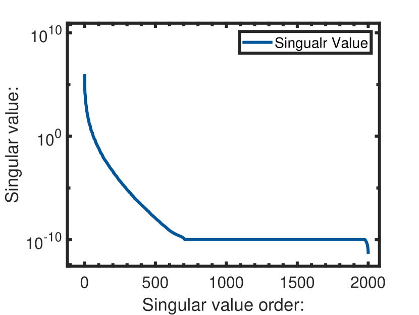
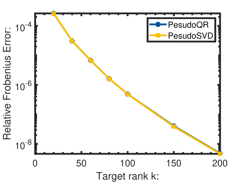
Refer to caption
Figure 4: Singular values of microConvection
Refer to caption
(a) Relative Frobenius Error
Refer to caption
(b) Running Time
Figure 5: Relative Errors and Running Time of CFD simulation with different target rank k𝑘k

Figure 6 illustrates that our compression can highly approximate the origin velocity field and compute the shear rates closely match the real data even if algorithm compress the original data from 256.81256.81256.81MB to 26.2826.2826.28MB.

Refer to caption
(a) Origin at 8th step
Refer to caption
(b) Recovered at 8th step
Refer to caption
(c) Origin at 14th step
Refer to caption
(d) Recovered at 14th step
Refer to caption
(e) Origin at 23rd step
Refer to caption
(f) Recovered at 23rd step
Figure 6: Shear rate computed from origin data and compressed data
Example 7.2.

In this section, we will compress the output of a 4D Lorenz-type chaotic system simulation by our randomized quaternion low-rank approximation algorithms. The chaotic system is as follows:

{dxdt=a(yx)ew,dydt=xzhy,dzdt=bxycz,dwdt=kydw,cases𝑑𝑥𝑑𝑡𝑎𝑦𝑥𝑒𝑤otherwise𝑑𝑦𝑑𝑡𝑥𝑧𝑦otherwise𝑑𝑧𝑑𝑡𝑏𝑥𝑦𝑐𝑧otherwise𝑑𝑤𝑑𝑡𝑘𝑦𝑑𝑤otherwise\begin{cases}\frac{dx}{dt}=a(y-x)-ew,\\ \frac{dy}{dt}=xz-hy,\\ \frac{dz}{dt}=b-xy-cz,\\ \frac{dw}{dt}=ky-dw,\end{cases}

where x𝑥x, y𝑦y, z𝑧z and w𝑤w are state variables and a𝑎a, b𝑏b, c𝑐c, d𝑑d, e𝑒e, hh are positive parameters of system. In our simulation, we set a=5𝑎5a=5, b=20𝑏20b=20, c=1𝑐1c=1, d=0.1𝑑0.1d=0.1, k=0.1𝑘0.1k=0.1, e=20.6𝑒20.6e=20.6, h=11h=1. And we set 100001000010000 initial state (x,y,z,w)𝑥𝑦𝑧𝑤(x,y,z,w) randomly from sphere (x,y,z,w)2=20subscriptnorm𝑥𝑦𝑧𝑤220\parallel(x,y,z,w)\parallel_{2}=20. Choosing 200020002000 time instance, we can obtain a 10000×200010000200010000\times 2000 quaternion matrix which record the information of solutions. The quaternion matrix has slower spectrum decay shown in figure 7.
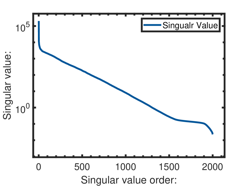
Refer to caption
Figure 7: Singular values of 4D Lorenz system

Figure 8 show that larger sketch size is necessary to obtain a high accuracy when input data have low spectrum decay. One-pass algorithms using pseudo-QR and pseduo-SVD have similar accuracy with the same sketch size. However, pseduo-QR may cost less time with larger sketch size.
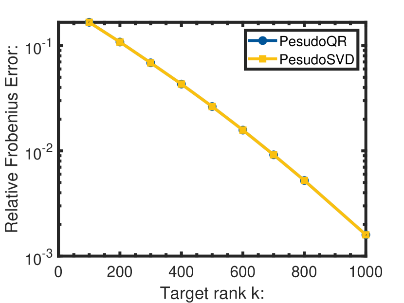
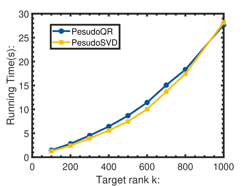
Refer to caption
(a) Relative Frobenius Error
Refer to caption
(b) Running Time
Figure 8: Relative Errors and Running Time of Lorenz system with different target rank k𝑘k

8 Conclusions

Existing quaternion rangefinders, which are based on quaternion orthogonalization, may be inefficient for large-scale problems. Based on the strategy of trading accuracy or space for speed, this work presented two practical rangefinders, which may not be orthonormal but still well-conditioned. The proposed rangefinders were then incorporated into the the one-pass algorithm proposed by Tropp et al. [41] for low-rank approximation to quaternion matrices. Throughout the whole algorithm, heavy quaternion computations has been transformed to QR, SVD, and solving linear equations in the complex arithmetic, such that mature scientific computing libraries or advanced algorithms can be employed to accelerate the computations. Theoretically, the probabilistic error bound was established; in particular, it was shown that the condition number of the rangefinder is proportional to the error, giving validity of using a non-orthonormal yet well-conditioned rangefinder. In addition, we established a deviation bound for the extreme singular values of a quaternion sub-Gaussian matrix, giving theoretical support of using a sub-Gaussian test matrix. Numerical experiments demonstrate that our algorithms work efficiently with less storage costs. Finally, we tested two practical numerical examples, including image dimensionality reduction and compression of large-scale scientific simulation data, to verify the effectiveness of the algorithm.

References

  • [1] Fast monte-carlo algorithms for finding low-rank approximations | Journal of the ACM. https://dl.acm.org/doi/abs/10.1145/1039488.1039494.
  • [2] Quaternion Matrix Compuation.
  • [3] E. Anderson, Z. Bai, C. Bischof, S. Blackford, J. Demmel, J. Dongarra, J. Du Croz, A. Greenbaum, S. Hammarling, A. McKenney, and D. Sorensen. LAPACK Users’ Guide. Society for Industrial and Applied Mathematics, Philadelphia, PA, third edition, 1999.
  • [4] Christos Boutsidis, David P. Woodruff, and Peilin Zhong. Optimal principal component analysis in distributed and streaming models. In Proceedings of the Forty-Eighth Annual ACM Symposium on Theory of Computing, STOC ’16, pages 236–249, New York, NY, USA, June 2016. Association for Computing Machinery.
  • [5] Angelika Bunse-Gerstner, Ralph Byers, and Volker Mehrmann. A quaternion QR algorithm. 55(1):83–95.
  • [6] Junren Chen and Michael K. Ng. Color image inpainting via robust pure quaternion matrix completion: Error bound and weighted loss. SIAM Journal on Imaging Sciences, 15(3):1469–1498, 2022.
  • [7] Yong Chen, Zhi-Gang Jia, Yan Peng, Ya-Xin Peng, and Dan Zhang. A new structure-preserving quaternion QR decomposition method for color image blind watermarking. 185:108088.
  • [8] Kenneth L. Clarkson and David P. Woodruff. Numerical linear algebra in the streaming model. In Proceedings of the Forty-First Annual ACM Symposium on Theory of Computing, pages 205–214, Bethesda MD USA, May 2009. ACM.
  • [9] Michael B. Cohen, Sam Elder, Cameron Musco, Christopher Musco, and Madalina Persu. Dimensionality reduction for k-means clustering and low rank approximation. In Proceedings of the Forty-Seventh Annual ACM Symposium on Theory of Computing, page 163–172, New York, NY, USA, 2015. Association for Computing Machinery.
  • [10] Intel Corporation. Intel math kernel library (version x.x). https://software.intel.com/content/www/us/en/develop/tools/math-kernel-library.html, 20xx. Accessed: yyyy-mm-dd.
  • [11] Todd A. Ell, Nicolas Le Bihan, and Stephen J. Sangwine. Quaternion Fourier Transforms. In Quaternion Fourier Transforms for Signal and Image Processing, pages 35–66. John Wiley & Sons, Ltd.
  • [12] Gene H. Golub and Charles F. Van Loan. Matrix Computations. Johns Hopkins Studies in the Mathematical Sciences. The Johns Hopkins University Press, fourth edition edition.
  • [13] T. N. E. Greville. Note on the Generalized Inverse of a Matrix Product. 8(4):518–521.
  • [14] N. Halko, P. G. Martinsson, and J. A. Tropp. Finding Structure with Randomness: Probabilistic Algorithms for Constructing Approximate Matrix Decompositions. 53(2):217–288.
  • [15] Nicholas J. Higham. Computing the Polar Decomposition—with Applications. SIAM Journal on Scientific and Statistical Computing, 7(4):1160–1174, 1986.
  • [16] Zhigang Jia, Michael K. Ng, and Guang-Jing Song. Lanczos method for large-scale quaternion singular value decomposition. Numerical Algorithms, 82(2):699–717, 2019.
  • [17] Zhigang Jia, Michael K. Ng, and Guang-Jing Song. Robust quaternion matrix completion with applications to image inpainting. Numerical Linear Algebra with Applications, 26(4):e2245, 2019.
  • [18] Zhigang Jia, Musheng Wei, and Sitao Ling. A new structure-preserving method for quaternion Hermitian eigenvalue problems. 239:12–24.
  • [19] Zhigang Jia, Musheng Wei, Mei-Xiang Zhao, and Yong Chen. A new real structure-preserving quaternion QR algorithm. 343(C):26–48.
  • [20] Ravindran Kannan and Santosh Vempala. Randomized algorithms in numerical linear algebra. Acta Numerica, 26:95–135, May 2017.
  • [21] Anastasia Kireeva and Joel A. Tropp. Randomized matrix computations: Themes and variations, February 2024.
  • [22] Nicolas Le Bihan and Jérôme Mars. Singular value decomposition of quaternion matrices: A new tool for vector-sensor signal processing. Signal Processing, 84(7):1177–1199, 2004.
  • [23] Chaoqian Li, Yonghe Liu, Fengsheng Wu, and Maolin Che. Randomized block Krylov subspace algorithms for low-rank quaternion matrix approximations.
  • [24] Ying Li, Musheng Wei, Fengxia Zhang, and Jianli Zhao. Real structure-preserving algorithms of Householder based transformations for quaternion matrices. 305:82–91.
  • [25] Ying Li, Musheng Wei, Fengxia Zhang, and Jianli Zhao. A fast structure-preserving method for computing the singular value decomposition of quaternion matrices. Applied Mathematics and Computation, 235:157–167, 2014.
  • [26] Ying Li, Musheng Wei, Fengxia Zhang, and Jianli Zhao. Real structure-preserving algorithms of Householder based transformations for quaternion matrices. Journal of Computational and Applied Mathematics, 305:82–91, October 2016.
  • [27] Qiaohua Liu, Sitao Ling, and Zhigang Jia. Randomized Quaternion Singular Value Decomposition for Low-Rank Matrix Approximation. 44(2):A870–A900.
  • [28] Yonghe Liu, Fengsheng Wu, Maolin Che, and Chaoqian Li. Fixed-precision randomized quaternion singular value decomposition algorithm for low-rank quaternion matrix approximations. Neurocomputing, 580:127490, May 2024.
  • [29] Chengyao Lyu, Junjun Pan, Michael K. Ng, and Xile Zhao. Randomized low rank approximation for nonnegative pure quaternion matrices. 150:108940.
  • [30] Michael W. Mahoney. Randomized Algorithms for Matrices and Data. Foundations and Trends® in Machine Learning, 3(2):123–224, November 2011.
  • [31] Per-Gunnar Martinsson and Joel Tropp. Randomized Numerical Linear Algebra: Foundations & Algorithms, March 2021.
  • [32] Per-Gunnar Martinsson and Joel A. Tropp. Randomized numerical linear algebra: Foundations and algorithms. Acta Numerica, 29:403–572, May 2020.
  • [33] Toshifumi Minemoto, Teijiro Isokawa, Haruhiko Nishimura, and Nobuyuki Matsui. Feed forward neural network with random quaternionic neurons. 136:59–68.
  • [34] Riley Murray, James Demmel, Michael W. Mahoney, N. Benjamin Erichson, Maksim Melnichenko, Osman Asif Malik, Laura Grigori, Piotr Luszczek, Michał Dereziński, Miles E. Lopes, Tianyu Liang, Hengrui Luo, and Jack Dongarra. Randomized Numerical Linear Algebra : A Perspective on the Field With an Eye to Software, April 2023.
  • [35] Huan Ren, Ru-Ru Ma, Qiaohua Liu, and Zheng-Jian Bai. Randomized Quaternion QLP Decomposition for Low-Rank Approximation. 92(3):80.
  • [36] Stephen J. Sangwine and Nicolas Le Bihan. Quaternion toolbox for MATLAB. http://qtfm.sourceforge.net/.
  • [37] Stephen J. Sangwine and Nicolas Le Bihan. Quaternion singular value decomposition based on bidiagonalization to a real or complex matrix using quaternion Householder transformations. Applied Mathematics and Computation, 182(1):727–738, November 2006.
  • [38] Soo-ChangPei, Ja-Han Chang, and Jian-Jiun Ding. Quaternion matrix singular value decomposition and its applications for color image processing. In Proceedings 2003 International Conference on Image Processing (Cat. No.03CH37429), volume 1, pages I–805–8. IEEE.
  • [39] Yanfeng Sun, Shangyou Chen, and Baocai Yin. Color face recognition based on quaternion matrix representation. 32(4):597–605.
  • [40] Joel A. Tropp and Robert J. Webber. Randomized algorithms for low-rank matrix approximation: Design, analysis, and applications, September 2023.
  • [41] Joel A. Tropp, Alp Yurtsever, Madeleine Udell, and Volkan Cevher. Practical Sketching Algorithms for Low-Rank Matrix Approximation. 38(4):1454–1485.
  • [42] Joel A. Tropp, Alp Yurtsever, Madeleine Udell, and Volkan Cevher. Streaming Low-Rank Matrix Approximation with an Application to Scientific Simulation. 41(4):A2430–A2463.
  • [43] Roman Vershynin. Introduction to the non-asymptotic analysis of random matrices. In Gitta Kutyniok and Yonina C. Eldar, editors, Compressed Sensing: Theory and Applications, pages 210–268. Cambridge University Press.
  • [44] Musheng Wei, Ying Li, Fengxia Zhang, and Jianli Zhao. Quaternion Matrix Computations. Nova Science Publishers, Incorporated, 2018.
  • [45] David P. Woodruff. Sketching as a Tool for Numerical Linear Algebra. Foundations and Trends® in Theoretical Computer Science, 10(1-2):1–157, 2014.
  • [46] Franco Woolfe, Edo Liberty, Vladimir Rokhlin, and Mark Tygert. A fast randomized algorithm for the approximation of matrices. Applied and Computational Harmonic Analysis, 25(3):335–366, November 2008.
  • [47] Fuzhen Zhang. Quaternions and matrices of quaternions. 251:21–57.
  • [48] Huisheng Zhang and Hui Lv. Augmented Quaternion Extreme Learning Machine. 7:90842–90850.
Proof of Theorem 3.3.

Let 𝐇=𝐔Σ𝐕𝐇𝐔Σsuperscript𝐕\mathbf{H}=\mathbf{U}\Sigma\mathbf{V}^{*} be a compact QSVD of 𝐇𝐇\mathbf{H} where Σ=diag(σ1,,σs)Σdiagsubscript𝜎1subscript𝜎𝑠\Sigma=\texttt{diag}(\sigma_{1},\ldots,\sigma_{s}) with σisubscript𝜎𝑖\sigma_{i} arranged in a decreasing order. Denote

f(x):=(1ϵ)x+ϵx1.assign𝑓𝑥1italic-ϵ𝑥italic-ϵsuperscript𝑥1f(x):=(1-\epsilon)x+\epsilon x^{-1}.

Then (6) shows that 𝐇newsubscript𝐇𝑛𝑒𝑤\mathbf{H}_{new} has singular values f(σi)=(1ϵ)σi+ϵσi1𝑓subscript𝜎𝑖1italic-ϵsubscript𝜎𝑖italic-ϵsuperscriptsubscript𝜎𝑖1f(\sigma_{i})=(1-\epsilon)\sigma_{i}+\epsilon{\sigma_{i}}^{-1}, i=1,,s𝑖1𝑠i=1,\ldots,s. We first consider the upper bound of f𝑓f on [σs,1]subscript𝜎𝑠1[\sigma_{s},1] and [1,σ1]1subscript𝜎1[1,\sigma_{1}], respectively.

For any ϵitalic-ϵ\epsilon and x[1,σ1]𝑥1subscript𝜎1x\in[1,\sigma_{1}],

f(x)=(1ϵ)x+ϵx1(1ϵ)x+ϵxx,𝑓𝑥1italic-ϵ𝑥italic-ϵsuperscript𝑥11italic-ϵ𝑥italic-ϵ𝑥𝑥f(x)=(1-\epsilon)x+\epsilon{x}^{-1}\leq(1-\epsilon)x+\epsilon x\leq x,

meaning that f(x)σ1𝑓𝑥subscript𝜎1f(x)\leq\sigma_{1} on [1,σ1]1subscript𝜎1[1,\sigma_{1}].

Next, we consider x[σs,1]𝑥subscript𝜎𝑠1x\in[\sigma_{s},1]. Observe that f(x)𝑓𝑥f(x) is convex when x>0𝑥0x>0, which achieves the maximal value on the boundary. It follows from ϵσsitalic-ϵsubscript𝜎𝑠\epsilon\geq\sigma_{s} that f(σs)(1ϵ)σs+σsσs11=f(1)𝑓subscript𝜎𝑠1italic-ϵsubscript𝜎𝑠subscript𝜎𝑠superscriptsubscript𝜎𝑠11𝑓1f(\sigma_{s})\geq(1-\epsilon)\sigma_{s}+\sigma_{s}\sigma_{s}^{-1}\geq 1=f(1), i.e., f𝑓f is upper bounded by f(σs)=(1ϵ)σs+ϵ/σs𝑓subscript𝜎𝑠1italic-ϵsubscript𝜎𝑠italic-ϵsubscript𝜎𝑠f(\sigma_{s})=\left(1-\epsilon\right)\sigma_{s}+\epsilon/\sigma_{s} on [σs,1]subscript𝜎𝑠1[\sigma_{s},1]. Furthermore, as σs1subscript𝜎𝑠1\sigma_{s}\leq 1 and ϵδσsitalic-ϵ𝛿subscript𝜎𝑠\epsilon\leq\delta\sigma_{s},

f(x)(1ϵ)σs+ϵ/σs(1δσs)σs+δσs/σs=δ+σsδσs2<δ+1/(4δ).𝑓𝑥1italic-ϵsubscript𝜎𝑠italic-ϵsubscript𝜎𝑠1𝛿subscript𝜎𝑠subscript𝜎𝑠𝛿subscript𝜎𝑠subscript𝜎𝑠𝛿subscript𝜎𝑠𝛿superscriptsubscript𝜎𝑠2𝛿14𝛿f(x)\leq\left(1-\epsilon\right)\sigma_{s}+\epsilon/\sigma_{s}\leq(1-\delta\sigma_{s})\sigma_{s}+\delta\sigma_{s}/\sigma_{s}=\delta+\sigma_{s}-\delta\sigma_{s}^{2}<\delta+1/(4\delta).

The analysis above together with σ12subscript𝜎12\sigma_{1}\leq\sqrt{2} in Theorem 3.2 shows that the largest singular value of 𝐇newsubscript𝐇𝑛𝑒𝑤\mathbf{H}_{new} cannot exceed max{2,δ+1/(4δ)}2𝛿14𝛿\max\{\sqrt{2},\delta+1/(4\delta)\}.

On the other hand, it follows from the convexity of f(x)𝑓𝑥f(x) that when x>0𝑥0x>0, f(x)2ϵ(1ϵ)𝑓𝑥2italic-ϵ1italic-ϵf(x)\geq 2\sqrt{\epsilon(1-\epsilon)}. The range of ϵitalic-ϵ\epsilon implies 2ϵ(1ϵ)2σs(1σs)2italic-ϵ1italic-ϵ2subscript𝜎𝑠1subscript𝜎𝑠2\sqrt{\epsilon(1-\epsilon)}\geq 2\sqrt{\sigma_{s}(1-\sigma_{s})}. Thus f(x)2σs(1σs)𝑓𝑥2subscript𝜎𝑠1subscript𝜎𝑠f(x)\geq 2\sqrt{\sigma_{s}(1-\sigma_{s})}.

We also need a lower bound on σssubscript𝜎𝑠\sigma_{s}. When κ(H)>max{22δ,2δ2+1/2}=2δmax{2,δ+1/(4δ)}2δσ1𝜅𝐻22𝛿2superscript𝛿2122𝛿2𝛿14𝛿2𝛿subscript𝜎1\kappa(H)>\max\{2\sqrt{2}\delta,2\delta^{2}+1/2\}=2\delta\max\{\sqrt{2},\delta+1/(4\delta)\}\geq 2\delta\sigma_{1}, we obtain that σs1/(2δ)subscript𝜎𝑠12𝛿\sigma_{s}\leq 1/\left(2\delta\right).

Comparing the two upper bounds on f𝑓f obtained previously, if σ1δ+1/(4δ)subscript𝜎1𝛿14𝛿\sigma_{1}\geq\delta+1/(4\delta),

κ(𝐇new)𝜅subscript𝐇𝑛𝑒𝑤\displaystyle\kappa(\mathbf{H}_{new}) σ12σs(1σs);absentsubscript𝜎12subscript𝜎𝑠1subscript𝜎𝑠\displaystyle\leq\frac{\sigma_{1}}{2\sqrt{\sigma_{s}\left(1-\sigma_{s}\right)}}; (47)

then

κ(𝐇new)κ(𝐇)σ12(1σs)σ1/2max{2,δ+1/(4δ)}/21,𝜅subscript𝐇𝑛𝑒𝑤𝜅𝐇subscript𝜎121subscript𝜎𝑠subscript𝜎122𝛿14𝛿21\displaystyle\frac{\kappa(\mathbf{H}_{new})}{\sqrt{\kappa(\mathbf{H})}}\leq\frac{\sqrt{\sigma_{1}}}{2\sqrt{\left(1-\sigma_{s}\right)}}\leq\sqrt{\sigma_{1}}/\sqrt{2}\leq\sqrt{\max\{\sqrt{2},\delta+1/(4\delta)\}}/\sqrt{2}\leq 1, (48)

where the second inequality follows from σs1/(2δ)<1/2subscript𝜎𝑠12𝛿12\sigma_{s}\leq 1/\left(2\delta\right)<1/2, and the last one comes from the range of δ𝛿\delta. Similarly, if σ1<δ+1/(4δ)subscript𝜎1𝛿14𝛿\sigma_{1}<\delta+1/(4\delta),

κ(𝐇new)𝜅subscript𝐇𝑛𝑒𝑤\displaystyle\kappa(\mathbf{H}_{new}) δ+1/(4δ)2σs(1σs);absent𝛿14𝛿2subscript𝜎𝑠1subscript𝜎𝑠\displaystyle\leq\frac{\delta+1/(4\delta)}{2\sqrt{\sigma_{s}\left(1-\sigma_{s}\right)}}; (49)

then

κ(𝐇new)κ(𝐇)δ+1/(4δ)2σ1(1σs)δ+1/(4δ)211/(2δ)<1,𝜅subscript𝐇𝑛𝑒𝑤𝜅𝐇𝛿14𝛿2subscript𝜎11subscript𝜎𝑠𝛿14𝛿2112𝛿1\displaystyle\frac{\kappa(\mathbf{H}_{new})}{\sqrt{\kappa(\mathbf{H})}}\leq\frac{\delta+1/(4\delta)}{2\sqrt{\sigma_{1}\left(1-\sigma_{s}\right)}}\leq\frac{\delta+1/(4\delta)}{2\sqrt{1-1/(2\delta)}}<1, (50)

where the second inequality follows from σ11subscript𝜎11\sigma_{1}\geq 1 and σs1/(2δ)subscript𝜎𝑠12𝛿\sigma_{s}\leq 1/\left(2\delta\right), while the last one comes from that δ+1/(4δ)211/(2δ)𝛿14𝛿2112𝛿\frac{\delta+1/(4\delta)}{2\sqrt{1-1/(2\delta)}} is non-decreasing on [1,7/2]172[1,\sqrt{7}/2]. The result follows.

Proof of Corollary 3.1.

Using the analysis in Theorem 3.3, one can use the induction method to show that if all the singular values σi(𝐇k)subscript𝜎𝑖subscript𝐇𝑘\sigma_{i}(\mathbf{H}_{k}) lies in [2σs(𝐇k1)(1σs(𝐇k1)),max{2,δ+1/(4δ)}]2subscript𝜎𝑠subscript𝐇𝑘11subscript𝜎𝑠subscript𝐇𝑘12𝛿14𝛿\left[2\sqrt{\sigma_{s}(\mathbf{H}_{k-1})(1-\sigma_{s}(\mathbf{H}_{k-1}))},\max\{\sqrt{2},\delta+1/(4\delta)\}\right], then all σi(𝐇k+1)subscript𝜎𝑖subscript𝐇𝑘1\sigma_{i}(\mathbf{H}_{k+1}) also lie in [2σs(𝐇k)(1σs(𝐇k)),max{2,δ+1/(4δ)}]2subscript𝜎𝑠subscript𝐇𝑘1subscript𝜎𝑠subscript𝐇𝑘2𝛿14𝛿[2\sqrt{\sigma_{s}(\mathbf{H}_{k})(1-\sigma_{s}(\mathbf{H}_{k}))},\max\{\sqrt{2},\delta+1/(4\delta)\}]. Similar to the proof of Theorem 3.3, κ(𝐇k+1)<κ(𝐇k)𝜅subscript𝐇𝑘1𝜅subscript𝐇𝑘\kappa(\mathbf{H}_{k+1})<\sqrt{\kappa(\mathbf{H}_{k})}. ∎

Proof of Proposition 3.1.

We first use the induction method to show that span(Ub~,𝒥Ub~¯)=2tspansubscript𝑈~𝑏𝒥¯subscript𝑈~𝑏2𝑡{\rm span}(U_{\tilde{b}},\mathcal{J}\overline{U_{\tilde{b}}})=2t. For t=1𝑡1t=1, this claim is true as u1𝒥u1¯perpendicular-tosubscript𝑢1𝒥¯subscript𝑢1u_{1}\perp\mathcal{J}\overline{u_{1}}. Suppose now that we have found Uk:=[ui1,,uik]Ub(k<t)assignsubscript𝑈𝑘subscript𝑢subscript𝑖1subscript𝑢subscript𝑖𝑘subscript𝑈𝑏𝑘𝑡U_{k}:=[u_{i_{1}},\ldots,u_{i_{k}}]\in U_{b}~{}(k<t) such that span(Uk,𝒥Uk¯)spansubscript𝑈𝑘𝒥¯subscript𝑈𝑘{\rm span}(U_{k},\mathcal{J}\overline{U_{k}}) has dimension 2k2𝑘2k. Note that Ubsubscript𝑈𝑏U_{b} is partially orthonormal and span(Ub)spansubscript𝑈𝑏{\rm span}(U_{b}) has dimension 2t>2k2𝑡2𝑘2t>2k, and so there always exists at least a uik+1UbUksubscript𝑢subscript𝑖𝑘1subscript𝑈𝑏subscript𝑈𝑘u_{i_{k+1}}\in U_{b}\setminus U_{k}, such that

uik+1span(Uk,𝒥Uk¯).subscript𝑢subscript𝑖𝑘1spansubscript𝑈𝑘𝒥¯subscript𝑈𝑘\displaystyle u_{i_{k+1}}\notin{\rm span}(U_{k},\mathcal{J}\overline{U_{k}}). (51)

We first show that (51) is equivalent to 𝒥uik+1¯span(Uk,𝒥Uk¯)𝒥¯subscript𝑢subscript𝑖𝑘1spansubscript𝑈𝑘𝒥¯subscript𝑈𝑘\mathcal{J}\overline{u_{i_{k+1}}}\notin{\rm span}(U_{k},\mathcal{J}\overline{U_{k}}). Suppose on the contrary that 𝒥uik+1¯span(Uk,𝒥Uk¯)𝒥¯subscript𝑢subscript𝑖𝑘1spansubscript𝑈𝑘𝒥¯subscript𝑈𝑘\mathcal{J}\overline{u_{i_{k+1}}}\in{\rm span}(U_{k},\mathcal{J}\overline{U_{k}}), which by Lemma 2.1 is equivalent to

uik+1¯=𝒥𝒥uik+1¯span(𝒥Uk,𝒥𝒥Uk¯)uik+1span(𝒥Uk¯,Uk),¯subscript𝑢subscript𝑖𝑘1superscript𝒥𝒥¯subscript𝑢subscript𝑖𝑘1spansuperscript𝒥subscript𝑈𝑘superscript𝒥𝒥¯subscript𝑈𝑘subscript𝑢subscript𝑖𝑘1span𝒥¯subscript𝑈𝑘subscript𝑈𝑘\displaystyle\overline{u_{i_{k+1}}}=\mathcal{J}^{*}\mathcal{J}\overline{u_{i_{k+1}}}\in{\rm span}(\mathcal{J}^{*}U_{k},\mathcal{J}^{*}\mathcal{J}\overline{U_{k}})\Leftrightarrow{u_{i_{k+1}}}\in{\rm span}(\mathcal{J}\overline{U_{k}},{U_{k}}),

deducing a contradiction.

Next, we will prove that span(Uk,𝒥Uk¯,uik+1,𝒥uik+1¯)spansubscript𝑈𝑘𝒥¯subscript𝑈𝑘subscript𝑢subscript𝑖𝑘1𝒥¯subscript𝑢subscript𝑖𝑘1{\rm span}(U_{k},\mathcal{J}\overline{U_{k}},u_{i_{k+1}},\mathcal{J}\overline{u_{i_{k+1}}}) has dimension 2(k+1)2𝑘12(k+1). Denote M:=[Uk,𝒥Uk]assign𝑀subscript𝑈𝑘𝒥subscript𝑈𝑘M:=[U_{k},\mathcal{J}U_{k}], PM:=MMassignsubscript𝑃𝑀𝑀superscript𝑀P_{M}:=MM^{\dagger}, and PM:=I2mMMassignsubscript𝑃superscript𝑀perpendicular-tosubscript𝐼2𝑚𝑀superscript𝑀P_{M^{\perp}}:=I_{2m}-MM^{\dagger} the orthogonal projection onto span(M)span𝑀{\rm span}(M) and span(M)spansuperscript𝑀perpendicular-to{\rm span}(M)^{\perp}, respectively. Then uik+1subscript𝑢subscript𝑖𝑘1u_{i_{k+1}} can be divided into two part:

PMuik+1span(M)perpendicular-tosubscript𝑃superscript𝑀perpendicular-tosubscript𝑢subscript𝑖𝑘1span𝑀\displaystyle P_{M^{\perp}}u_{i_{k+1}}\perp{\rm span}(M)\quad andPMuik+1span(M).andsubscript𝑃𝑀subscript𝑢subscript𝑖𝑘1span𝑀\displaystyle\text{and}\quad P_{M}u_{i_{k+1}}\in{\rm span}(M). (52)

Correspondingly, 𝒥uik+1¯𝒥¯subscript𝑢subscript𝑖𝑘1\mathcal{J}\overline{u_{i_{k+1}}} can be divided into PM𝒥uik+1¯subscript𝑃superscript𝑀perpendicular-to𝒥¯subscript𝑢subscript𝑖𝑘1P_{M^{\perp}}\mathcal{J}\overline{u_{i_{k+1}}} and PM𝒥uik+1¯subscript𝑃𝑀𝒥¯subscript𝑢subscript𝑖𝑘1P_{M}\mathcal{J}\overline{u_{i_{k+1}}}, where we also notice that

𝒥PMuik+1¯=𝒥uik+1¯𝒥PM¯uik+1¯=𝒥uik+1¯PM𝒥uik+1¯=PM𝒥uik+1¯,𝒥¯subscript𝑃superscript𝑀perpendicular-tosubscript𝑢subscript𝑖𝑘1𝒥¯subscript𝑢subscript𝑖𝑘1𝒥¯subscript𝑃𝑀¯subscript𝑢subscript𝑖𝑘1𝒥¯subscript𝑢subscript𝑖𝑘1subscript𝑃𝑀𝒥¯subscript𝑢subscript𝑖𝑘1subscript𝑃superscript𝑀perpendicular-to𝒥¯subscript𝑢subscript𝑖𝑘1\displaystyle\mathcal{J}\overline{P_{M^{\perp}}u_{i_{k+1}}}=\mathcal{J}\overline{u_{i_{k+1}}}-\mathcal{J}\overline{P_{M}}\overline{u_{i_{k+1}}}=\mathcal{J}\overline{u_{i_{k+1}}}-P_{M}\mathcal{J}\overline{u_{i_{k+1}}}=P_{M^{\perp}}\mathcal{J}\overline{u_{i_{k+1}}},

with the second equality from Lemma 2.3.

By Lemma 2.1, PMuik+1𝒥PMuik+1¯perpendicular-tosubscript𝑃superscript𝑀perpendicular-tosubscript𝑢subscript𝑖𝑘1𝒥¯subscript𝑃superscript𝑀perpendicular-tosubscript𝑢subscript𝑖𝑘1P_{M^{\perp}}u_{i_{k+1}}\perp\mathcal{J}\overline{P_{M^{\perp}}u_{i_{k+1}}}, and due to the above relation, 𝒥PMuik+1¯Mperpendicular-to𝒥¯subscript𝑃superscript𝑀perpendicular-tosubscript𝑢subscript𝑖𝑘1𝑀\mathcal{J}\overline{P_{M^{\perp}}u_{i_{k+1}}}\perp M. Thus,

span(M,PMuik+1,PM𝒥uik+1¯)=span(M,PMuik+1,𝒥PMuik+1¯)span𝑀subscript𝑃superscript𝑀perpendicular-tosubscript𝑢subscript𝑖𝑘1subscript𝑃superscript𝑀perpendicular-to𝒥¯subscript𝑢subscript𝑖𝑘1span𝑀subscript𝑃superscript𝑀perpendicular-tosubscript𝑢subscript𝑖𝑘1𝒥¯subscript𝑃superscript𝑀perpendicular-tosubscript𝑢subscript𝑖𝑘1{\rm span}(M,P_{M^{\perp}}u_{i_{k+1}},P_{M^{\perp}}\mathcal{J}\overline{u_{i_{k+1}}})={\rm span}(M,P_{M^{\perp}}u_{i_{k+1}},\mathcal{J}\overline{P_{M^{\perp}}u_{i_{k+1}}})

has dimension 2(k+1)2𝑘12(k+1). Therefore,

span(Uk,𝒥Uk¯,uik+1,𝒥uik+1¯)spansubscript𝑈𝑘𝒥¯subscript𝑈𝑘subscript𝑢subscript𝑖𝑘1𝒥¯subscript𝑢subscript𝑖𝑘1\displaystyle{\rm span}(U_{k},\mathcal{J}\overline{U_{k}},u_{i_{k+1}},\mathcal{J}\overline{u_{i_{k+1}}})
=\displaystyle= span(M,PMuik+1+PMuik+1,PM𝒥uik+1¯+PM𝒥uik+1¯)span𝑀subscript𝑃superscript𝑀perpendicular-tosubscript𝑢subscript𝑖𝑘1subscript𝑃𝑀subscript𝑢subscript𝑖𝑘1subscript𝑃𝑀𝒥¯subscript𝑢subscript𝑖𝑘1subscript𝑃superscript𝑀perpendicular-to𝒥¯subscript𝑢subscript𝑖𝑘1\displaystyle{\rm span}(M,P_{M^{\perp}}u_{i_{k+1}}+P_{M}u_{i_{k+1}},P_{M}\mathcal{J}\overline{u_{i_{k+1}}}+P_{M^{\perp}}\mathcal{J}\overline{u_{i_{k+1}}})

also has dimension 2(k+1)2𝑘12(k+1). Thus the induction method shows that there exists Ub~=[ui1,,uit]Ubsubscript𝑈~𝑏subscript𝑢subscript𝑖1subscript𝑢subscript𝑖𝑡subscript𝑈𝑏U_{\tilde{b}}=[u_{i_{1}},\ldots,u_{i_{t}}]\in U_{b}, such that span(Ub~,𝒥Ub~)spansubscript𝑈~𝑏𝒥subscript𝑈~𝑏{\rm span}(U_{\tilde{b}},\mathcal{J}U_{\tilde{b}}) has dimension 2t2𝑡2t.

It is obvious that (Ub~)(Ub)subscript𝑈~𝑏subscript𝑈𝑏\mathcal{R}(U_{\tilde{b}})\subset\mathcal{R}(U_{b}). Furthermore, for any u𝑢u in Ub~subscript𝑈~𝑏U_{\tilde{b}} corresponding to singular value σ𝜎\sigma of χ𝐘subscript𝜒𝐘{\chi}_{\mathbf{Y}}, 𝒥u¯𝒥¯𝑢\mathcal{J}\overline{u} is also corresponding to σ𝜎\sigma. which means that (𝒥Ub~¯)(Ub)𝒥¯subscript𝑈~𝑏subscript𝑈𝑏\mathcal{R}(\mathcal{J}\overline{U_{\tilde{b}}})\subset\mathcal{R}(U_{b}). Recall that (Ub)subscript𝑈𝑏\mathcal{R}(U_{b}) also has dimension 2t2𝑡2t; thus (Ub~,𝒥Ub~¯)=(Ub)subscript𝑈~𝑏𝒥¯subscript𝑈~𝑏subscript𝑈𝑏\mathcal{R}(U_{\tilde{b}},\mathcal{J}\overline{U_{\tilde{b}}})=\mathcal{R}(U_{b}). ∎