Eigenvector distributions and optimal shrinkage estimators for large covariance and precision matrices
Abstract
This paper focuses on investigating Stein’s invariant shrinkage estimators for large sample covariance matrices and precision matrices in high-dimensional settings. We consider models that have nearly arbitrary population covariance matrices, including those with potential spikes. By imposing mild technical assumptions, we establish the asymptotic limits of the shrinkers for a wide range of loss functions. A key contribution of this work, enabling the derivation of the limits of the shrinkers, is a novel result concerning the asymptotic distributions of the non-spiked eigenvectors of the sample covariance matrices, which can be of independent interest.
1 Introduction
Estimating large covariance matrices and their inverses, the precision matrices, is fundamental in modern data analysis. It is well-known that in the high-dimensional regime when the data dimension is comparable to or even larger than the sample size the sample covariance matrices and their inverses are poor estimators [71]. To obtain consistent estimators, many structural assumptions have been imposed, such as sparse or banded structures. Based on these assumptions, many regularization methods have been developed to obtain better estimators. We refer the readers to [20, 36, 62] for a more comprehensive review.
Although these structural assumptions are useful for many applications, they may not be applicable in general scenarios. In this paper, we consider the estimation of the population covariance matrix and its inverse, denoted by , through Stein’s (orthogonally or rotationally) invariant estimators [64, 65] without imposing (almost) any specific structural assumption. Given a data matrix and its sample covariance matrix , we say and are invariant estimators for and respectively, if they satisfy that
| (1.1) |
for any orthogonal matrix For an illustration, we take the covariance matrix estimation as an example. Denote the eigenvalues and corresponding eigenvectors of by and . Stein [64, 65] showed that the optimal invariant estimator for satisfy
| (1.2) |
where commonly referred to as shrinkers, are some nonlinear functionals depending on the choice of the loss function the sample covariance matrix , and the population covariance matrix For many loss functions , the random quantities ’s have closed forms (see Appendix A) so that the estimation problem reduces to finding efficient estimators or estimable convergent limits for ’s. As demonstrated in Appendix A, usually takes the following form:
| (1.3) |
where is a function depending on , or the following form when :
| (1.4) |
Here, represents the eigenmatrix associated with the zero eigenvalues of . In the classical setting when is fixed, Stein derived consistent estimators for (1.3) under various loss functions; we refer the readers to [63] in this regard.
In the current paper, we investigate this problem in the high-dimensional regime when is comparable to in the sense that there exists a constant such that
| (1.5) |
Note that we allow for so that the inverse of the sample covariance matrix may not exist in general. We also treat our models with general and possibly spiked population covariance matrices (up to some mild technical assumptions). This substantially generalizes Johnstone’s spiked covariance matrix model [41], where the non-spiked eigenvalues are assumed to be unity (see (1.6) below).
In the general model setup and under the condition (1.5), we provide analytical and closed-form formulas to characterize the convergent limits of (1.3) and (1.4) for both the spiked and non-spiked eigenvectors . These limits can be further estimated consistently and adaptively for various choices of loss functions (or equivalently, the function ). One crucial step involves studying the asymptotic distributions for the sample eigenvectors , which can be of significant independent interest. In what follows, we first discuss some related works on the shrinkers’ estimation for the regime (1.5) in Section 1.1. Then, we review some relevant literature about the eigenvector distributions of some classical random matrix models in Section 1.2. Finally, we provide an overview of the contributions of this paper and highlight some main novelties in Section 1.3.
1.1 Related works on shrinker estimation
We now provide a brief review of some previous results concerning the estimation of the shrinkers in the high-dimensional regime. In [32], the authors considered Johnstone’s spiked covariance matrix model with
| (1.6) |
where is the rank of signals. By replacing Stein’s original estimator (1.2) with the stronger rank-aware assumption for (see equation (1.13) therein), [32] provided analytical and closed-form convergent limits for the shrinkers , , under various choices of loss functions when . These convergent limits can be consistently estimated using the first eigenvalues and eigenvectors of An important insight conveyed by [32] is that the selection of the loss function can have a significant impact on the estimation of shrinkers. Nevertheless, the assumption for is crucial for their theory, which fails when in (1.6) is replaced by a general positive definite covariance matrix . To address this issue, under Stein’s setup (1.2) and using Frobenius norm as the loss function, Bun [18] derived the convergent limits for shrinkers associated with the spikes of a general covariance matrix and provide an adaptive estimation of these limits.
On the other hand, the derivation of the convergent limits for shrinkers associated with non-spiked eigenvectors becomes much more challenging and is substantially different from [32, 18]. In this context, adaptive estimations for the shrinkers still can be provided, see e.g., [49, 50, 53, 52], but theoretically, they are consistent only in an averaged sense. The main challenge lies in the fact that a key theoretical input is the limiting eigenvector empirical spectral distribution derived in [49], which is insufficient for deriving the convergent limits and providing consistent estimators for individual shrinkers.
Inspired by these earlier works, in this paper, we will rigorously prove the convergent limits for all the (spiked or non-spiked) shrinkers associated with general spiked covariance matrix models in (2.2) below for various loss functions. Roughly speaking, our generalized model extends (1.6) by replacing with an (almost) arbitrary positive definite covariance matrix, introducing a more realistic modeling approach. Note that the framework in [32] is not applicable in this setting. We will also provide consistent estimators for individual shrinkers by approximating these convergent limits with sample quantities. From a technical viewpoint, our current paper improves all previous results in the existing literature.
1.2 Related works on eigenvector distributions of sample covariance matrices
Next, we briefly review some previous results concerning eigenvector distributions of random matrices, with a focus on the sample covariance matrices. On the global level, the eigenvector empirical spectral distribution (VESD) has been extensively investigated under various assumptions on the population covariance matrices, as explored in studies such as [3, 69, 66, 67]. Notably, these papers demonstrated that the limiting VESD is closely linked to the Marchenko-Pastur (MP) law [56]. Building upon these results, investigations into the distributions of the linear spectral statistics (LSS) of the eigenvectors have been conducted under various settings in [3, 69]. Specifically, it has been established that the LSS of the eigenvectors exhibit asymptotic Gaussian behavior under almost arbitrary population covariance .
On the local level, an important result was established in [15] when , demonstrating that the projection of any eigenvector onto an arbitrary deterministic unit vector converges in law to a standard normal distribution after a proper normalization. In particular, this implies that all the eigenvector entries are asymptotically Gaussian. Furthermore, in [15], the concept of quantum unique ergodicity (QUE) for eigenvectors was also established based on these findings. Similar results were obtained for the non-outlier eigenvectors under Johnstone’s spiked covariance matrix model (1.6) in [13], while the distributions of outlier eigenvectors were studied in [5, 7, 60]. For the case of a general diagonal population covariance matrix , the universality of eigenvector distributions was established both in the bulk and near the edge in [26]. However, the explicit distribution remains unknown.
Motivated by our specific applications in shrinkage estimation, our goal is to derive the explicit distributions for all eigenvectors of the non-spiked model, as well as the non-outlier eigenvectors of the spiked model, considering the assumption of a general population covariance matrix . These results have been lacking in the existing literature, as indicated by the aforementioned overview. To achieve this, we draw inspiration from recent advancements in the analysis of eigenvectors of Wigner matrices, as presented in [10, 11, 15, 44, 57].
1.3 An overview of our results and technical novelties
In this subsection, we present an overview of our results and highlight the main novelties of our work. Our main contributions can be divided into two parts: the convergent limit of each individual shrinker for various loss functions under the general spiked covariance model (see Section 2.2); the asymptotic eigenvector distributions for sample covariance matrices with general covariance structures (see Section 2.3).
For the convergence of shrinkers, under a general spiked covariance matrix model, we present explicit and closed-form formulas that characterize the convergent limit of each individual shrinker under various loss functions. The precise statement of this result can be found in Theorem 2.4. Notably, these formulas remain applicable even in the singular case with . Corollary 2.5 provides simplified versions of these formulas for specific choices of the loss function. Leveraging these theoretical findings, we establish the asymptotic risks associated with shrinkage estimation of covariance and precision matrices under various loss functions in Corollary 2.6. To facilitate practical implementation, we also introduce adaptive and consistent estimators for the convergent limits of the shrinkers, as outlined in Theorem 3.2. An package 111An online demo for the package can be found at https://xcding1212.github.io/RMT4DS.html has been developed to implement our methods.
Now, we will delve into the technical details concerning the derivation of the convergent limits of (1.3); the derivation of the limit of (1.4) is considerably simpler. The proofs for the spiked and non-spiked shrinkers exhibit notable differences. In the case of spiked shrinkers, we employ a decomposition of (1.3) into two components: a low-rank part and a high-rank part, as illustrated in equation (4.2) below. The low-rank portion can be effectively approximated by leveraging the convergence limits of the outlier eigenvalues and eigenvectors, as demonstrated in Lemma B.7. On the other hand, the high-rank component takes the form of , , where are some deterministic weights and are the eigenvectors of The existing literature (e.g., [45, 27]) provides a ”rough” delocalization bound like with high probability, for any small constant . However, this bound is insufficient for our specific purpose. To address this issue, consider the resolvent (or Green’s function) of defined as for . Then, we will conduct a higher order resolvent expansion to obtain that (c.f. Lemma B.8)
where is the convergent limit of the -th outlier eigenvalue of and denotes certain deterministic weights. Now, our focus narrows down to estimating the random variable given by In the special case where Bun [18] has provided an estimation of this quantity utilizing a concentration inequality. However, in this paper, we employ a variational approach that simplifies the estimation process and enables the computation of the limit for any sequence of weights ; see (C.6) for further details.
On the other hand, for the non-spiked shrinkers , , the above approach fails. Instead, we need to directly evaluate by establishing what is known as a QUE estimate. In the case where , this form has been investigated in [13] utilizing the methodology developed in [15]. In this work, we establish the QUE for the non-spiked eigenvectors of under an almost arbitrary population covariance matrix . The key lies in establishing the asymptotic distributions for all non-outlier eigenvectors (c.f. Theorem 2.8), from which the QUE estimate can be derived (c.f. Theorem 2.12). The proof of the eigenvector distributions in this work builds upon and extends the eigenvector moment flow (EMF) approach introduced in [15], which involves three main steps. In the first step, we establish the local laws for the resolvent of . In the second step, we study the EMF for the rectangular matrix Dyson Brownian motion (DBM) of defined as , where represents the data matrix and is a matrix consisting of i.i.d. Brownian motions of variance . We demonstrate the relaxation of the EMF dynamics to equilibrium when , from which we can establish the Gaussian normality for the eigenvectors of . Finally, in the last step, we show that the eigenvector distributions of are close to those of , which is achieved through a standard Green’s function comparison argument. For a more detailed discussion of the above strategy, we direct readers to Section 4. Notably, this approach has been recently employed to establish the asymptotic distributions of eigenvalues and eigenvectors for various random matrix ensembles featuring general population covariance or variance profiles, as evidenced in works such as [10, 11, 31, 57, 16].
In our setting, Step 1 has already been accomplished in [45]. Moving on to Step 2, following the idea of [15], we establish in Theorem 4.5 that a general functional , encoding the joint moments of the projections of the eigenvectors of , relaxes to equilibrium with high probability on the time scale . This equilibrium characterizes the joint moments of a multivariate normal distribution, which concludes Step 2 by the moment method (c.f. Lemma 4.1). We remark that the proof of Theorem 4.5 relies on a probabilistic description of as the solution to a system of coupled SDEs representing a specific interacting particle system (c.f. Lemma 4.10). Since the current paper is motivated by applications in shrinker estimation, we specifically focus on investigating the joint distribution of eigenvectors projected onto a single direction, as illustrated in (4.7). Nevertheless, as discussed in Remark 2.9, our results can be extended to scenarios where different eigenvectors are projected onto multiple distinct directions. In such cases, it becomes necessary to consider a more complex interacting particle system.
One technical innovation of our proof is the comparison argument in Step 3 (see Lemma 4.2). In the existing literature (e.g., [13, 44]), the comparison is typically made between two random matrices, say and , where has the same covariance structure or variance profile as , but with entries that are Gaussian divisible (roughly speaking, we will set and ). However, this argument is applicable in our context only when the population covariance matrix is diagonal, as demonstrated in [26]. To address this issue, we introduce a new comparison approach by introducing an additional intermediate matrix as defined in (4.8). The matrix possesses the same covariance structure as while incorporating the randomness in . Moreover, for a fixed , we can carefully choose in such a way that it has the same law as . Then, to conclude Step 3, we will introduce a novel interpolation between and . Specifically, we define a continuous sequence of matrices , (see (4.10) for the precise definition). These matrices are specifically selected so that follows the distribution of , while follows the distribution of . Notably, unlike previous comparison arguments in the literature, during the transition from to , only the deterministic covariance structure of the interpolating matrices varies with . Finally, the comparison is conducted by controlling the derivative of the relevant quantities with respect to . For a more comprehensive explanation, readers can refer to the discussion below (4.9).
Outline of the paper. In this paper, we focus on the spiked covariance matrix model with a general population covariance. In Section 2, we introduce this model and state our main results, which are divided into two parts: in Section 2.2, we present the asymptotics of shrinkers; in Section 2.3, we provide results concerning the eigenvector distributions. In Section 3, we introduce adaptive and consistent estimators for the shrinkers and conduct numerical simulations to demonstrate the superior performance of our estimators. In Section 4, we discuss our proof strategy and highlight the technical novelties. All the technical proofs of the main results are given in Appendices B–F. For the convenience of readers, in Appendix A, we summarize some commonly used loss functions and the related shrinkers.
Notations. To facilitate the presentation, we introduce some necessary notations that will be used in this paper. We are interested in the asymptotic regime with . When we refer to a constant, it will not depend on or . Unless otherwise specified, we will use to denote generic large positive constants, whose values may change from line to line. Similarly, we will use , , , etc. to denote generic small positive constants. For any two sequences and depending on , , or means that for some constant , whereas or means that as . We say that if and . Moreover, for a sequence of random variables and non-negative quantities , we use to mean that is stochastically bounded and use to mean that converges to zero in probability. Denote by the upper half complex plane and the positive real line. For an event , we let or denote its indicator function. We use to denote the standard basis of certain Euclidean space, whose dimension will be clear from the context. For any , we denote and abbreviate . Given two (complex) vectors and , we denote their inner product by We use , , to denote the -norm of . Given a matrix , we use and , and to denote the operator, Hilbert-Schmidt, and maximum norms, respectively. We also use to denote the “generalized entries” of .
Acknowledgments. The authors want to thank Jun Yin for many helpful discussions. XCD is partially supported by NSF DMS-2114379 and DMS-2306439. YL and FY are partially supported by the National Key R&D Program of China (No. 2023YFA1010400).
2 Main results
2.1 The model and main assumptions
In this paper, we consider the non-spiked population covariance matrix , which is a deterministic positive definite matrix. Suppose it has a spectral decomposition
| (2.1) |
where is the diagonal matrix of eigenvalues arranged in the descending order, and denotes the eigenmatrix, i.e., the collection of the eigenvectors . In the statistical literature, people are also interested in finite rank deformations of by adding a fixed number of spikes to . Following [19, 27, 29], we define the spiked population covariance matrix as
| (2.2) |
Here, for the sequence of eigenvalues , we assume that there exists a fixed and a non-negative sequence such that
| (2.3) |
In other words, the first eigenvalues , , are the spiked eigenvalues with spiked strengths characterized by . Accordingly, we define the non-spiked and spiked sample covariance matrices considered in this paper as
| (2.4) |
where is a random data matrix with i.i.d. entries of mean zero and variance In our proof, we will also frequently use their companions:
| (2.5) |
Note (resp. ) has the same nonzero eigenvalues as (resp. ). In this paper, we will often regard the non-spiked model as a special case of the spiked one with .
In this paper, we study the asymptotic behavior of the models and using the Stieltjes transform method. Given any symmetric matrix , we denote its empirical spectral density (ESD) as
where , , denote the eigenvalues of . Given a probability measure on , we define its Stieltjes transform as
| (2.6) |
When , we adopt the convention that . It is well-known that the Stieltjes transform of the ESD of has the same asymptotics as the so-called deformed Marchenko-Pastur (MP) law [56]. It may include a Dirac delta mass at zero, for example, when or when for some . Furthermore, on can be determined by its Stieltjes transform . More precisely, define the function as
| (2.7) |
(As a convention, we let when .) For any fixed , there exists a unique solution to the self-consistent equation
| (2.8) |
see [45, Lemma 2.2] or the book [2] for more details. Then, we can determine the MP density from as
| (2.9) |
We summarize some basic facts about the support of in the following lemma.
Lemma 2.1 (Lemma 2.5 of [45] and Lemma 2.4 of [28]).
The support of is a disjoint union of connected components on
| (2.10) |
where is an integer that depends only on the ESD of , and we shall call the spectral edges of . Here, can be characterized as follows: there exists a real sequence such that are real solutions to the equations
Following the convention in the random matrix theory literature, we denote the rightmost and leftmost edges by and , respectively. For any , we define
| (2.11) |
which is the classical number of eigenvalues in . As a convention, we set . It has been shown in [45, Lemma A.1] that for . We now introduce the quantiles of , which are indeed the classical locations for the eigenvalues of .
Definition 2.2.
We define the classical eigenvalue locations (or the quantiles) of the deformed Marchenco-Pastur law as the unique solution to the equation
| (2.12) |
where we have abbreviated . Note that is well-defined since the ’s are integers. As a convention, we set for .
Now, we are ready to state the main assumptions for our results.
Assumption 2.3.
We assume the following assumptions hold.
-
(i)
On dimensionality. There exists a small constant such that (1.5) holds and
(2.13) -
(ii)
On in (2.4). For suppose that are i.i.d. real random variables with and In addition, we assume that the entries of have arbitrarily high moments: for each fixed , there exists a constant such that
(2.14) Finally, we assume that the entries of have vanishing third moments, i.e., .
- (iii)
-
(iv)
On the spikes in (2.3). There exists a fixed integer and a constant such that
(2.18) Moreover, the spikes are distinct in the sense that We also assume that the largest spike is bounded from above by .
Let us now provide a brief discussion on the above assumption. Condition (1.5) of part (i) means that we are considering the high-dimensional regime in this paper. We remark that in related works such as [32, 50, 52], it is required that converges to a fixed constant as . In comparison, our assumption (1.5) is more flexible and purely data-dependent. The condition (2.13) is introduced to avoid the occurrence of the “hard edge” phenomenon in the deformed MP law , that is, as . In fact, by the properties of the MP law [56], it is known that
| (2.19) |
The condition (2.13) is relatively mild since when , we can always omit certain samples to ensure that . Additionally, it is worth mentioning that even when , all our results remain valid for eigenvectors with indices up to , which correspond to the eigenvalues away from the hard edge .
Part (ii) imposes some moment conditions on the entries of . We remark that the high moment condition (2.14) can be relaxed to a certain extent—we may only assume that (2.14) holds for with being an absolute constant (e.g., ). Additionally, the vanishing third-moment condition is not essential, and it can be eliminated using an alternative approach distinct from our current proof. However, due to limitations in length, we will not explore this direction in the present paper, leaving it for future investigation.
For part (iii), the condition (2.15) is seen to be mild. The conditions (2.16) and (2.17) are some technical regularity conditions imposed on the ESD of . The edge regularity condition (2.16) has previously appeared (in slightly different forms) in several works on sample covariance matrices [6, 33, 40, 45, 54, 58], and it ensures a regular square-root behavior of the density near the spectral edges . The bulk regularity condition (2.17) was introduced in [45], and it imposes a lower bound on the asymptotic density of eigenvalues away from the edges. Both of these conditions are satisfied by “generic” population covariance matrices ; see e.g., the discussions in [45, Examples 2.8 and 2.9].
Finally, condition (2.18) in part (iv) means that , , are the supercritical spikes concerning the BBP transition [4] of the largest few eigenvalues of . In particular, they will give rise to outlier sample eigenvalues beyond the right edge of ; see e.g., Theorem 3.6 of [29]. It is possible to extend our results to the more general case with the sharper condition: for a small constant ,
(It is known that is the critical regime for BBP transition.) We can also allow for degenerate spikes and spikes that diverge with as . However, for brevity, we do not pursue such generalizations in this paper.
2.2 Asymptotics of optimal shrinkage estimators
In this subsection, we state the main statistical results on the analytical formulas and asymptotic risks for the optimal shrinkage estimators. Our first result concerns the asymptotics of the shrinkers. To state it, we now introduce more notations. For defined in (2.7) and we denote
| (2.20) |
(We will see in Lemma B.7 that is the classical location (i.e., convergent limit) of the -th outlier eigenvalue .) As noted in (1.3) and (1.4), the optimal shrinkers usually depend on the loss function via some continuous function on . Given such a function , for small, and , we define
| (2.21) |
We further define as in (2.8) by replacing with , that is, solves the following self-consistent equation:
| (2.22) |
Note when , we have and . We then denote the partial derivative of in as
| (2.23) |
By differentiating the equation (2.22) with respect to and at , we obtain that
| (2.24) |
From these two equations, we can derive the following explicit expression for :
| (2.25) |
By abbreviating , we now define
| (2.26) |
and the function
| (2.27) |
where for any two vectors , we denote
| (2.28) |
Here, we adopt the convention that for .
In this paper, we denote the eigenvalues of the non-spiked sample covariance matrix by and those of the spiked version by . To facilitate the presentation and with a slight abuse of notation, we will use the notation to represent the sample eigenvectors of either or . Additionally, we denote by the eigenmatrix associated with the zero eigenvalues of or . The specific model being referred to will be evident from the context. Now, we are ready to state the main results. First, we provide the convergent limits of the shrinkers.
Theorem 2.4.
Suppose Assumption 2.3 holds. Recall that are the quantiles of defined in Definition 2.2. For any continuous function defined on , the following estimates hold:
| (2.29) | ||||
| (2.30) | ||||
| (2.31) |
The above results (2.30) and (2.31) also extend to the non-spiked model with .
Theorem 2.4 provides a closed-form, analytic, and deterministic formula for the convergent limits of the shrinkage estimators. As summarized in Appendix A, commonly used loss functions include , etc. Our result gives the asymptotics of the shrinkers with exact dependence on the loss functions, the population eigenvalues, the classical eigenvalue locations, and the aspect ratio . In Section 3.1, we will provide numerical algorithms to estimate the aforementioned quantities consistently with sample quantities. Shrinkage estimators for other random matrix models have also been studied to some extent; see e.g., [9, 19, 39, 55]. We believe that our strategies and arguments can be extended and applied to these models with some modifications. We will explore this direction in future studies.
In the special case with (corresponding to the loss functions of Frobenius, minimal variance, disutility, and inverse Stein norms), the formulas of or will be significantly simplified, as shown in the following result.
Corollary 2.5.
Compared with Theorem 2.4, we have simpler and more implementable formulas in the case of . Notably, the unobserved quantities depend only on the Stieltjes transform and the classical eigenvalue locations or . As we will see in Section 3.1 and Appendix B, can be well approximated by the Stieltjes transform of the ESD of or due to the local laws of their resolvents, and and can be efficiently estimated by their sample counterparts using the convergence of outlier eigenvalues and the rigidity of non-outlier eigenvalues. These estimations only rely on the sample eigenvalues of or , which significantly simplifies our numerical algorithms.
Before concluding this section, we establish the asymptotic risks (or generalization errors) for Stein’s estimator under 12 commonly used loss functions as summarized in Appendix A.
Corollary 2.6.
Suppose Assumption 2.3 holds. Recall (2.26) and (2.27). Given a function , define for , for , and for . Let denote the optimal invariant estimators for as defined in (1.2). For the loss functions given in Table 1 below, the following estimates hold with probability .
-
(i)
For with we have that with probability ,
where , and are the shorthand notations for the Frobenius, inverse Stein, disutility, and minimum variance norms, respectively.
-
(ii)
For with we have that with probability ,
where and are the shorthand notations for the inverse Frobenius, Stein, and weighted Frobenius norms, respectively.
-
(iii)
For with we have that with probability ,
where means the Fréchet norm.
-
(iv)
For with we have that with probability ,
where means the Log-Euclidean norm.
-
(v)
Define , with , , , and . Then, we have that with probability ,
where and are the shorthand notations for the quadratic, inverse quadratic, and symmetrized Stein norms, respectively.
2.3 Eigenvector distributions for sample covariance matrices
In this subsection, we present the theoretical results regarding the asymptotic distributions of the non-outlier eigenvectors of (non-spiked or spiked) sample covariance matrices. For simplicity of presentation, we adopt the notion of “asymptotic equality in distribution”, as defined in [5, Definition 2.2].
Definition 2.7.
Two sequences of random vectors are asymptotically equal in distribution, denoted by if they are tight (i.e., for any there exists a such that ) and satisfy
for any bounded smooth function
Theorem 2.8 (Eigenvector distribution).
Suppose Assumption 2.3 holds. Given a deterministic unit vector and any fixed integer , take a subset of indices for the spiked model. Define the diagonal matrix
| (2.35) |
where is defined in (2.28) and are defined in Definition 2.2. Then, we have that
| (2.36) |
where are independent centered Gaussian random variables with variances . Equivalently, we can express (2.36) as
| (2.37) |
where are i.i.d. uniformly random signs independent of . The above result also extends to the non-spiked model with .
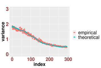
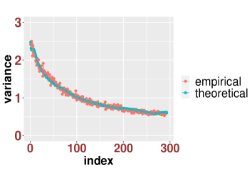
Theorem 2.8 provides a characterization of the joint distribution of the projections (referred to as “generalized components”) of the non-outlier eigenvectors from the non-spiked or spiked sample covariance matrices. It demonstrates that the generalized components of different eigenvectors are asymptotically independent Gaussian variables, and their variances can be explicitly computed. Given that eigenvectors are defined only up to a phase, we express the distributions of eigenvectors using the forms presented in (2.36) or (2.37). As a specific example, when , we can verify that by using the explicit form of solved from (2.8). This reduces to the result in [13, Theorem 2.20]. We provide numerical illustrations of Theorem 2.8 in Figure 2.1.
Remark 2.9.
For the sake of statistical applications and to maintain simplicity in our presentation, we have focused on a scenario where the sample eigenvectors are projected onto the same direction . However, as discussed in Remark D.3 below, our results can be extended to situations where different sample eigenvectors are projected onto multiple distinct directions. More precisely, our method can be generalized to show that for deterministic unit vectors , ,
| (2.38) |
Such a result has recently been established for Wigner matrices in [57], and we believe similar arguments can be applied to our setting. However, since (2.38) falls beyond the scope of the current paper, we intend to pursue it in future research.
Remark 2.10.
In the current paper, our focus regarding the spiked model has been on the distribution of its non-outlier eigenvectors. As for the outlier eigenvectors, we only examine their first-order asymptotics (see Lemmas B.7 and B.8), which suffice for our statistical applications. It is important to note that the derivation of their asymptotic distributions relies on a totally different approach from that for Theorem 2.8, which will be explained in more detail in Section 4.1. In the case where , the distributions of outlier eigenvectors have been extensively studied in [5]. Unlike Theorem 2.8, the results in [5] demonstrate that the distribution of the generalized components of outlier eigenvectors generally involves a linear combination of Gaussian and Chi-square random variables. Nevertheless, we believe that by following the approach in [5] and utilizing some tools developed in our paper, we can derive the distribution of all outlier eigenvectors for general . Finally, we remark that the methods presented in our paper can be applied to study the eigenvector distribution in other important statistical models, such as those discussed in [38, 37]. Exploring these directions will be the focus of our future work.
Remark 2.11.
Motivated by the applications in covariance matrix estimation, we have focused on demonstrating the eigenvector distributions for the sample covariance matrices defined in (2.4), specifically the distribution of the left singular vectors of the data matrix. However, in applications such as spectral clustering, there is also interest in the right singular vectors. Fortunately, by virtue of symmetry, our arguments can be readily extended to study the eigenvectors of and in (2.5) with minor modifications. For the sake of simplicity, we will not explore this direction in the present paper.
During the proof of Theorem 2.8, we can derive the following concentration inequality for the weighted average of the generalized components of eigenvectors, known as the quantum unique ergodicity estimate [10, 15]. This result plays a key role in the proof of Theorem 2.4.
Theorem 2.12 (Quantum unique ergodicity).
Let be a deterministic sequence of real values such that for all . Recall that are the eigenvectors of . Then, there exists a constant such that for any and each , the following estimate holds:
| (2.39) |
The above result also extends to the non-spiked model with .
In the literature, Theorem 2.12 is sometimes called a “weak” form of QUE since both the probability bound and the rate in estimate (2.39) are non-optimal. Recently, a stronger notion of QUE called the eigenstate thermalization hypothesis has also been established for Wigner matrices [23, 1, 24, 25, 21, 22]. We conjecture that a similar form should also hold for sample covariance matrices, in the sense that
We plan to explore this direction in future works.
3 Adaptive and consistent estimators for shrinkers
In Section 2.2, we have provided the formulas for the convergent limits of the shrinkers . However, in practical applications, the quantities involved in (2.20)–(2.28) are typically unknown and need to be estimated. In this section, we propose adaptive and consistent estimators for these quantities, which in turn provide consistent estimators for the shrinkers . Our focus will be on the possibly spiked model, which encompasses the non-spiked model as a special case with .
3.1 Data-driven estimators for the shrinkers
As one can see, estimating the quantities in (2.20)–(2.28) requires consistent estimation of the spectrum of the non-spiked eigenvalues of . In the literature, this problem has been addressed for non-spiked sample covariance matrices in [42, 46] based on the sample eigenvalues of . For the spiked sample covariance matrix model, we know that the non-outlier eigenvalues of stick to those of as indicated by equation (B.23) below. Consequently, we can substitute the non-outlier eigenvalues , , into the algorithms from [42, 46] to obtain estimators for the eigenvalues of , denoted as
| (3.1) |
In particular, they provide consistent estimation of the spectrum of the non-spiked eigenvalues , . To facilitate ease of use for users, these algorithms can be implemented using the functions (for the method in [42]) or (for the method in [46]) in our package. Next, we turn to the estimation of the quantities associated with the spikes of . For , we let
| (3.2) |
where and are defined as
| (3.3) |
For a small constant , we define
| (3.4) |
Then, we introduce the following estimator of :
Note all the above quantities can be computed adaptively using the observed sample covariance matrix Moreover, the next result shows that they are consistent estimators for the relevant quantities.
Lemma 3.1.
Under Assumption 2.3, the ESD of converges weakly to , that is, for each ,
| (3.5) |
For any continuous function defined on , there exists a small constant such that for any and ,
| (3.6) |
With the above lemma, we can propose a consistent estimator for in (2.26) as
| (3.7) |
Next, we propose a consistent estimator for in (2.27). Corresponding to in (2.28), we define
| (3.8) |
where and are defined as follows with :
| (3.9) |
With the above notations, we then define that for and small ,
| (3.10) |
Now, we are prepared to present the consistency result for our proposed estimators of the shrinkers.
Theorem 3.2.
Under Assumption 2.3, for any continuous function defined on , there exists a small constant such that for any ,
| (3.11) |
| (3.12) |
Combining Theorem 3.2 and Theorem 2.4, we see that , , and can be used to consistently estimate the shrinkers and their associated asymptotic risks for various loss functions (see Corollary 2.6). These estimators are constructed in a data-driven manner and can be implemented easily. In Section 3.2, we conduct extensive numerical simulations to demonstrate the effectiveness of our proposed estimators. Also notice that by employing (3.8), we are able to estimate the variances in (2.35) for the eigenvector distribution stated in Theorem 2.8.
When we can provide more straightforward estimators for the simplified formulas presented in Corollary 2.5. With the notations in (3.3) and (3.9), we define
Notably, all these estimators do not involve the estimated non-outlier eigenvalues in (3.1).
Lemma 3.3.
Remark 3.4.
In the construction of the estimators for shrinkers, we assume that the number of spikes is known. However, in practical applications, this assumption is often unrealistic. Fortunately, it has been demonstrated in [29, 31, 43, 59] that can be estimated consistently using the eigenvalues under item (iv) of Assumption 2.3. To facilitate the convenience of our readers, we have included a function called in the package, which can be used to estimate .
3.2 Numerical simulations
In this section, we employ Monte-Carlo simulations to demonstrate the effectiveness of our proposed estimators for the loss functions corresponding to or .
3.2.1 Setup
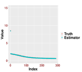
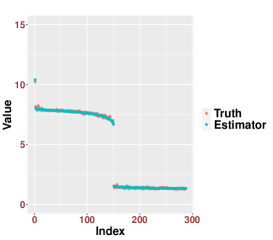
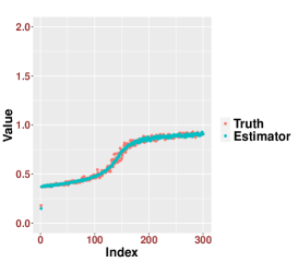
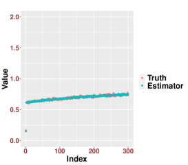
In the simulations, we generate with i.i.d. Gaussian random variables that satisfy item (ii) of Assumption 2.3. As for the population covariance matrix , we consider the following four alternatives:
-
(i)
takes the form (2.2), where is an orthogonal matrix generated from the function and is defined as
-
(ii)
takes the form (2.2), where is an orthogonal matrix generated from the function , and is defined as where represents real numbers evenly distributed within the interval .
-
(iii)
is a spiked matrix with a single spike equal to 9, and is a Toeplitz matrix with for .
-
(iv)
takes the form (2.2), where is an orthogonal matrix generated from the function , and is defined as
We would like to highlight that in our simulations, the support of the MP law consists of a single component (i.e., in (2.10)) for settings (i)–(iii), and two bulk components (i.e., in (2.10)) for setting (iv).
Regarding the loss functions, we consider those associated with and As stated in Corollary 2.6 (or Lemma A.1 below), corresponds to the Frobenius, inverse Stein, disutility, and minimum variance loss functions, while corresponds to the Stein, weighted Frobenius, and inverse Frobenius loss functions.
3.2.2 Performance of our estimators
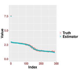
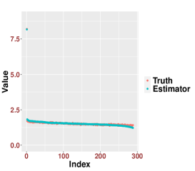
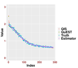
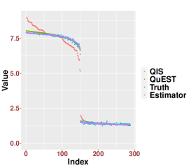
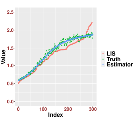
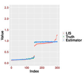
We proceed to evaluate the performance of our estimators for the shrinkers . To compute the quantity in (3.9), we select . In order to facilitate visual interpretation, we present our results for in Figure 3.1 and for in Figure 3.2. It is evident that the estimators outlined in Theorem 3.2 and Lemma 3.3 yield accurate predictions for the shrinkers across all simulation scenarios, encompassing different loss functions associated with or .
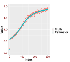
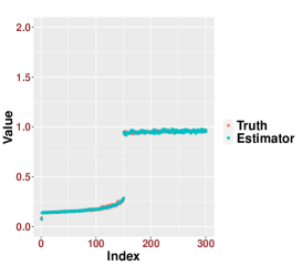
3.2.3 Comparison with other methods
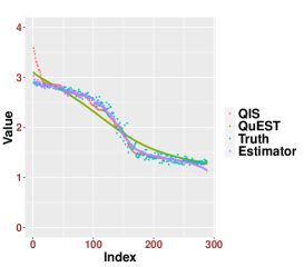
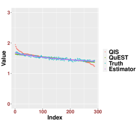
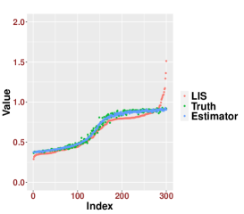
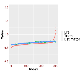
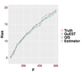
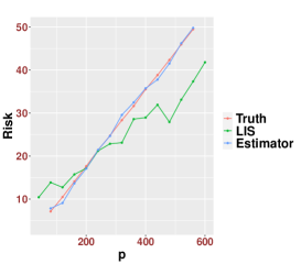
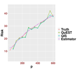
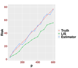
Next, we compare our proposed estimators with the existing methods for estimating shrinkers proposed by Ledoit and Wolf. For we compare our method (Estimator) with the recently proposed quadratic-inverse shrinkage estimator (QIS) [53]222The codes can be found at https://github.com/MikeWolf007/covShrinkage/blob/main/qis.R and the QuEST method based on numerically solving equation (2.8) [51].333The QuEST method can be implemented using the package For the only existing method is the LIS method proposed in [53].444The codes can be found at https://github.com/MikeWolf007/covShrinkage/blob/main/lis.R Since all these methods focus on non-spiked models, we remove the spikes from the four settings described in Section 3.2.1 for comparison.
First, we visually compare the plots of different estimators of the shrinkers in Figures 3.3 and 3.4. Our proposed estimators demonstrate superior accuracy in all settings and for both forms of . The performance of the other estimators depends on the specific underlying population covariance matrix and the chosen loss function. Second, in Figure 3.5, we assess the accuracy of different estimators in predicting the generalization errors, as stated in Corollary 2.6. Our proposed estimators provide the most accurate predictions. It is worth noting that the competing methods perform well when , but their performance deteriorates when .
4 Proof strategy and key technical ingredients
4.1 Outline of the proof strategy
In this subsection, we outline the proof strategy. We focus on the more challenging term in (1.3), while the term in (1.4) is considerably simpler to deal with. We rewrite (1.3) as
| (4.1) |
where recall that and are the eigenvectors of the population and sample covariance matrices and , respectively. The analysis of outlier and non-outlier eigenvectors in the spiked model relies on different strategies. The study of outlier eigenvectors is based on a standard perturbation argument. Under item (iv) of Assumption 2.3, the outlier eigenvalues are well separated from the bulk of the spectrum (see Lemma B.7 below). Therefore, using Cauchy’s integral formula, the generalized components of the outlier eigenvectors can be represented as a contour integral of the generalized components of the resolvents, which can be well approximated using the anisotropic local law (c.f. Section B.1).
Specifically, for , we decompose (4.1) as
| (4.2) |
On one hand, according to Lemma B.7 below, the first term on the right-hand side (RHS) of (4.2) is dominated by the term since is negligible for . The term can be further estimated using the asymptotic behavior of and described in Lemma B.7. On the other hand, for the second term on the RHS of (4.2), since there are terms in the summation, existing delocalization results in the literature—, —are no longer sufficient for our proof. Instead, we need to derive higher-order asymptotics for . In (B.26) below, we will show that with high probability,
where represents the resolvent associated with the non-spiked model (see Remark B.4 below for the precise definition). By estimating the first term on the RHS using a variational argument and the local laws of , we obtain the asymptotic limit for the second term on the RHS of (4.2) and complete the proof. Further details can be found in the discussion below (C.3).
Next, we describe the strategy for studying the non-outlier eigenvectors, which differs significantly from the approach used for the outlier eigenvectors and is essentially non-perturbative. Let be the eigenvectors of . By noting that , we can focus on the model and study the asymptotic properties of its singular vectors. Let be a Gaussian random matrix that is independent of . Its entries are i.i.d. centered Gaussian random variables with variance . For we define a matrix Dyson Brownian motion as
| (4.3) |
The matrix might not be precisely equal to (although in the proof below, we will consider it as a perturbation of ). To account for this, we introduce a new notation for the initial condition, denoting it as , where will be chosen later and is a diagonal matrix with eigenvalues that satisfy the conditions for in 2.3. In other words, consists of a non-spiked part with eigenvalues satisfying item (iii) of 2.3, while the spikes of satisfy item (iv) of 2.3. Then, we denote the sample covariance matrix of by
| (4.4) |
and let and be the associated eigenvalues and eigenvectors of , respectively. As shown in [31, 30], the non-outlier eigenvalues of follow a rectangular Dyson Brownian motion, whose limiting density is given by the rectangular free convolution of the ESD of with the MP law at time . Similar to Definition 2.2, we denote by the classical eigenvalue locations for . (For the definitions of and , we refer readers to the discussion around (B.33) in the appendix, where corresponds to .) Corresponding to (2.28), for and vectors we define the function
| (4.5) |
where is defined as in (2.8) with replaced by .
Our proof strategy for the non-outlier eigenvectors consists of two steps. In the first step, we establish the eigenvector distribution for on a small time scale , where is a small positive constant. In the second step, we introduce a novel comparison argument to show that the eigenvector distribution of at time is asymptotically equal to the distribution at . These two steps together establish the asymptotic distribution of the eigenvectors of the original matrix for properly chosen . For the first step, we will prove the following counterpart of Theorem 2.8 for .
Lemma 4.1.
Suppose Assumption 2.3 holds (when ). Take for an arbitrary constant . Given a deterministic unit vector and a subset of indices for a fixed integer , define the diagonal matrix
| (4.6) |
Then, we have that
| (4.7) |
where are i.i.d. uniformly random signs independent of .
The proof of Lemma 4.1 will be outlined in Section 4.2. It is based on a careful analysis of the eigenvector moment flow for , and the main result of the analysis is summarized in Theorem 4.5.
For the second step, we will establish the following comparison result, which shows that the distributions of the non-outlier eigenvectors of coincide with those of when we carefully select . Note that the proof of Theorem 2.8 is completed by combining Lemma 4.2 with Lemma 4.1.
Lemma 4.2.
Suppose Assumption 2.3 holds. Fix a time for a small constant . We choose . For a fixed integer , let be a smooth function satisfying that
for a constant and all satisfying . Then, given any deterministic unit vector and an arbitrary subset of indices , there exists a constant such that
where and are the eigenvectors of and , respectively.
The proof of Lemma 4.2 will be outlined in Section 4.3. In the proof, we introduce the auxiliary matrix
| (4.8) |
We choose the non-spiked parts of and as and , respectively. We denote the sample covariance matrix of as and its eigenvectors as . We aim to prove that for any ,
| (4.9) |
This completes the proof of Lemma 4.2 by taking , in which case we have as .
To prove (4.9), we will utilize a functional integral representation formula in terms of the resolvents, as presented in Lemma 4.11, and a novel comparison argument in Lemma 4.12 below. Now, we discuss briefly the new comparison strategy. In the literature (e.g., [13, 26, 44]), when establishing the universality for the singular vector distributions of , people typically compare the representation formula for directly with that for . Let be an independent copy of . Due to the rotational invariance of the distribution of , has the same law as , whose non-outlier eigenvector distributions have been provided in Lemma 4.1. In the previous comparison approach between and , people often applied the Lindeberg replacement (or other interpolations) to replace the entries of step by step with the entries of in the representation formula, controlling the error at each step using the local laws of the related resolvents. However, this approach fails for our setting—a direct application of the comparison idea (as in [26, 44]) leads to uncontrollable errors. To address this issue, we propose a novel interpolation method that establishes a connection between and as varies from 0 to 1:
| (4.10) |
Here, represents a continuous sequence of Bernoulli random matrices with i.i.d. Bernoulli random entries, represents the Hadamard product, , and . Under this choice, we can verify that , and has the same law as , leveraging the rotational invariance of the distribution of . As a result, our analysis will focus on the deterministic covariance structure rather than the random components and .
4.2 Eigenvector moment flow and proof of Lemma 4.1
The objective of this section is to prove Lemma 4.1 by analyzing the eigenvector moment flow (EMF) of in (4.4), building upon the idea in [15]. We first introduce some new notations before discussing the key ideas for the proof.
For any deterministic unit vector as in Lemma 4.1, we define Moreover, we use the notation and denote the filtration of -algebras up to time by
| (4.11) |
Inspired by [15, 31], we consider observables of the form
| (4.12) |
where we set for the non-spiked model and for the spiked model. Here, represents a fixed configuration, and we can interpret as the number of particles at site . This interpretation allows us to view the EMF as an interacting particle system later. The factor corresponds precisely to the -th moment of a standard Gaussian random variable, and we adopt the convention that . Clearly, is a functional encoding joint moments of the generalized components of the non-outlier eigenvectors.
Before delving into the analysis of let us provide some heuristics as to why the asymptotic variance takes the form presented in (4.6). For simplicity, we consider the single-particle case where for some . In this scenario, we have For , using the spectral decomposition of , we find that on the local scale of order
| (4.13) |
Drawing inspiration from the results for Wigner matrices [15], we expect that the random variables are asymptotically independent, and that the distributions of and are close to each other when . Guided by this intuition, we expect that that should closely resemble the averaged quantity in (4.13) due to the law of large numbers, as long as we choose .
Next, we show that the left-hand side (LHS) of (4.13) can be effectively approximated by as defined in (4.5). First, using the local laws presented in Lemma B.9 and Remark B.10 below, the LHS of (4.13) has a deterministic limit, denoted as
| (4.14) |
for , where denotes the non-spiked part of . By setting , , and , we obtain the formula in (4.5) with . (This is also why we use the same notation in (4.5) and (4.14).) Moreover, by the eigenvalue rigidity property of stated in Lemma B.9 below, we know that is well-approximated by with high probability. Therefore, by choosing and , according to the above discussion, we expect that when ,
This gives the desired result for the single-particle case. For general configuration, using the above argument we heuristically expect that
| (4.15) |
In general, establishing the asymptotic distribution of can be accomplished by demonstrating that its finite-dimensional moments asymptotically match those of a random vector composed of independent Chi-squared random variables with the desired variances. To make the above heuristics rigorous, we will work with the following smoothed version of in the actual proof.
Definition 4.3.
Given the deterministic unit vector , let be defined as in (4.5). Let be a smooth, non-negative function supported in such that . For any constant , we define and the function as the convolution
| (4.16) |
Then, for any fixed configuration , we define
| (4.17) |
Remark 4.4.
We remark that the function is defined in terms of and rather than and . The usage of instead of is due to certain technical considerations, which will become apparent in the technical derivation (E.40) below. Using the definition of and the estimate (B.18) in the appendix, it can be readily observed that for any small constant ,
| (4.18) |
The following EMF result shows that converges to the equilibrium at a time scale of as long as we choose sufficiently small.
Theorem 4.5.
Under the setting of Lemma 4.1, choose for some constants and . Then, for any fixed and , there exist (small) positive constants such that
where denotes the total number of particles.
Lemma 4.6.
Under the setting of Lemma 4.1, take for an arbitrary constant . Then, for any fixed , there exist (small) positive constants such that
Proof.
We are now ready to prove Lemma 4.1 by combining the results in Theorem 4.5 and Lemma 4.6.
Proof of Lemma 4.1.
Let be a configuration supported on . Note that the functional in (4.12) encodes the joint moments of the random variables . By employing Theorem 4.5 and Lemma 4.6, we establish that these joint moments match the corresponding finite-dimensional joint moments of where are i.i.d. centered Gaussian random variables having the desired variances . This concludes the proof using the standard method of moments. ∎
Remark 4.7.
In Theorem 4.5, we have chosen , which yields an almost sharp speed of convergence to local equilibrium for the edge eigenvalues and eigenvectors (see e.g., [15, 48, 31]). However, this rate is suboptimal for the convergence of bulk eigenvalues and eigenvectors. Indeed, it has been demonstrated in [15, 10] that the bulk eigenvectors of Wigner matrices converge to local equilibrium once , and we anticipate that similar results extend to sample covariance matrices as well. Since this aspect is not the primary focus of the current paper, we will refrain from delving into this direction here.
The proof of Theorem 4.5 can be found in Appendix E. The main ingredient is a probabilistic description of the EMF of as a multi-particle random walk in a random environment. The random environment is described by the well-studied Dyson Brownian motion of the eigenvalues. Let be a matrix where , and , are independent standard Brownian motions. For any , in (4.3) can be rewritten as
| (4.19) |
We refer to this type of dynamics as a rectangular DBM. Under (4.19), Lemma 4.9 provides the stochastic differential equations (SDEs) that describe the evolution of eigenvalues and eigenvectors of . Note that when . To account for this, we introduce the following equivalence relation.
Definition 4.8 (Equivalence relation).
We define the following equivalence relation on : if and only if or . In particular, when , simply means .
Lemma 4.9.
The eigenvalues and eigenvectors of satisfy the following SDEs:
| (4.20) |
| (4.21) |
where and , , are independent standard Brownian motions. (Note that has the same distribution as , although they generally correspond to different matrix Brownian motions.) We will refer to (4.20) and (4.21) as DBM and eigenvector flow, respectively. Their initial conditions at are given by and .
Proof.
We extend the definition (4.12) to
| (4.22) |
for the particle configuration . For , we introduce the notation
| (4.23) |
which denotes the particle configuration obtained by moving one particle from site to site , given that . The following lemma defines the main object of study—the eigenvector moment flow. Its proof will be presented in Appendix D.
Lemma 4.10.
4.3 Green’s function comparison and proof of Lemma 4.2
As discussed below Lemma 4.2, in order to complete the proof, it suffices to prove the comparison estimate (4.9). Inspired by the works [13, 26, 44], we first establish a functional integral representation formula for the generalized components of the non-outlier eigenvectors, expressed in terms of the resolvents of either the non-spiked or spiked model.
We first introduce some new notations. For any let denote an indicator function of the interval smoothed on the scale More precisely, is a smooth function satisfying the following properties: (1) for , (2) for , and (3)
| (4.27) |
For any positive integer , let be a smooth cutoff function such that
| (4.28) |
For any , if , then we define
| (4.29) |
where recall that is defined in (2.11) and the choice of is due to the rigidity of eigenvalues in (B.37) below. Now, for any constants and , we define
| (4.30) |
and the intervals (recall that are defined above (4.5))
| (4.31) |
Corresponding to the function defined above, we abbreviate
| (4.32) |
Finally, for any , we define
| (4.33) |
where recall that and were defined in (4.4) and (4.8), respectively.
Now, we are ready to state the key functional representation formula for the generalized components of non-outlier eigenvectors. The proof of this formula will be presented in Appendix F.1.
Lemma 4.11.
Under the setting of Lemma 4.2, for any , there exists a small constant such that the following estimate holds for sufficiently small constants , , and :
A similar estimate holds for , , and .
With Lemma 4.11, proving (4.9) boils down to showing that the two representation formulas involving the resolvents of and are asymptotically equal to each other. As discussed below (4.9), this is achieved through a novel comparison argument based on the interpolation (4.10). Correspondingly, we define the family of interpolating sample covariance matrices as
| (4.34) |
Here, “” means “equal in distribution”. Let be defined as in (4.33) using The following lemma provides the Green’s function comparison result, which, together with Lemma 4.11, concludes the proof of (4.9).
Lemma 4.12.
To establish (4.36), we will control the derivative of with respect to . More details can be found in Appendix F.2. Now, we are ready to conclude the proof of Lemma 4.2 by combining the above two lemmas.
Proof of Lemma 4.2.
When , it is straightforward to check that the condition (4.35) holds with for and defined below (4.10). Then, by applying Lemma 4.11 and Lemma 4.12, we obtain (4.9), which further concludes the proof of Lemma 4.2 by setting and . ∎
References
- [1] A. Adhikari, S. Dubova, C. Xu, and J. Yin. Eigenstate thermalization hypothesis for generalized Wigner matrices. arXiv preprint arXiv:2302.00157, 2023.
- [2] Z. Bai and J. W. Silverstein. Spectral analysis of large dimensional random matrices. Springer Series in Statistics. Springer, New York, second edition, 2010.
- [3] Z. D. Bai, B. Q. Miao, and G. M. Pan. On asymptotics of eigenvectors of large sample covariance matrix. The Annals of Probability, 35(4):1532–1572, 2007.
- [4] J. Baik, G. Ben Arous, and S. Péché. Phase transition of the largest eigenvalue for nonnull complex sample covariance matrices. Ann. Probab., 33(5):1643–1697, 2005.
- [5] Z. Bao, X. Ding, J. Wang, and K. Wang. Statistical inference for principal components of spiked covariance matrices. The Annals of Statistics, 50(2):1144–1169, 2022.
- [6] Z. Bao, G. Pan, and W. Zhou. Universality for the largest eigenvalue of sample covariance matrices with general population. Ann. Statist., 43:382–421, 2015.
- [7] Z. Bao and D. Wang. Eigenvector distribution in the critical regime of BBP transition. Probability Theory and Related Fields, 182(1-2):399–479, 2022.
- [8] F. Benaych-Georges, C. Bordenave, M. Capitaine, C. Donati-Martin, A. Knowles, D. Chafaï, S. Péché, and B. de Tilière. Advanced Topics in Random Matrices. Panoramas et synthèses - Société mathématique de France. Société mathématique de France, 2017.
- [9] F. Benaych-Georges, J.-P. Bouchaud, and M. Potters. Optimal cleaning for singular values of cross-covariance matrices. The Annals of Applied Probability, 33(2):1295–1326, 2023.
- [10] L. Benigni. Eigenvectors distribution and quantum unique ergodicity for deformed Wigner matrices. Annales de l’Institut Henri Poincaré, Probabilités et Statistiques, 56(4):2822–2867, 2020.
- [11] L. Benigni and P. Lopatto. Optimal delocalization for generalized Wigner matrices. Advances in Mathematics, 396:108109, 2022.
- [12] A. Bloemendal, L. Erdős, A. Knowles, H.-T. Yau, and J. Yin. Isotropic local laws for sample covariance and generalized Wigner matrices. Electronic Journal of Probability, 19(none):1 – 53, 2014.
- [13] A. Bloemendal, A. Knowles, H.-T. Yau, and J. Yin. On the principal components of sample covariance matrices. Probability theory and related fields, 164(1):459–552, 2016.
- [14] P. Bourgade, L. Erdös, and H.-T. Yau. Edge universality of beta ensembles. Communications in Mathematical Physics, 332(1):261–353, 2014.
- [15] P. Bourgade and H.-T. Yau. The eigenvector moment flow and local quantum unique ergodicity. Communications in Mathematical Physics, 350(1):231–278, 2017.
- [16] P. Bourgade, H.-T. Yau, and J. Yin. Random band matrices in the delocalized phase I: Quantum unique ergodicity and universality. Comm. Pure Appl. Math., 73(7):1526–1596, 2020.
- [17] M.-F. Bru. Diffusions of perturbed principal component analysis. Journal of multivariate analysis, 29(1):127–136, 1989.
- [18] J. Bun. An optimal rotational invariant estimator for general covariance matrices: The outliers. Preprint, 2018.
- [19] J. Bun, J.-P. Bouchaud, and M. Potters. Cleaning large correlation matrices: tools from random matrix theory. Physics Reports, 666:1–109, 2017.
- [20] T. T. Cai, Z. Ren, and H. H. Zhou. Estimating structured high-dimensional covariance and precision matrices: Optimal rates and adaptive estimation. Electronic Journal of Statistics, 10(1):1 – 59, 2016.
- [21] G. Cipolloni, L. Erdős, and J. Henheik. Eigenstate thermalisation at the edge for Wigner matrices. arXiv preprint arXiv:2309.05488, 2023.
- [22] G. Cipolloni, L. Erdős, J. Henheik, and O. Kolupaiev. Gaussian fluctuations in the equipartition principle for Wigner matrices. Forum of Mathematics, Sigma, 11:e74, 2023.
- [23] G. Cipolloni, L. Erdős, and D. Schröder. Eigenstate thermalization hypothesis for Wigner matrices. Communications in Mathematical Physics, 388(2):1005–1048, 2021.
- [24] G. Cipolloni, L. Erdős, and D. Schröder. Normal fluctuation in quantum ergodicity for Wigner matrices. The Annals of Probability, 50(3):984–1012, 2022.
- [25] G. Cipolloni, L. Erdős, and D. Schröder. Thermalisation for Wigner matrices. Journal of Functional Analysis, 282(8):109394, 2022.
- [26] X. Ding. Singular vector distribution of sample covariance matrices. Advances in applied probability, 51(1):236–267, 2019.
- [27] X. Ding. Spiked sample covariance matrices with possibly multiple bulk components. Random Matrices: Theory and Applications, 10(01):2150014, 2021.
- [28] X. Ding and F. Yang. A necessary and sufficient condition for edge universality at the largest singular values of covariance matrices. Annals of Applied Probability, 28(3):1679–1738, 2018.
- [29] X. Ding and F. Yang. Spiked separable covariance matrices and principal components. The Annals of Statistics, 49(2):1113–1138, 2021.
- [30] X. Ding and F. Yang. Edge statistics of large dimensional deformed rectangular matrices. Journal of Multivariate Analysis, page 105051, 2022.
- [31] X. Ding and F. Yang. Tracy-Widom distribution for heterogeneous Gram matrices with applications in signal detection. IEEE Transactions on Information Theory, 68(10):6682–6715, 2022.
- [32] D. Donoho, M. Gavish, and I. Johnstone. Optimal shrinkage of eigenvalues in the spiked covariance model. Annals of Statistics, 46(4):1742–1778, 2018.
- [33] N. El Karoui. Tracy-Widom limit for the largest eigenvalue of a large class of complex sample covariance matrices. Ann. Probab., 35(2):663–714, 2007.
- [34] L. Erdős, A. Knowles, and H.-T. Yau. Averaging fluctuations in resolvents of random band matrices. Ann. Henri Poincaré, 14:1837–1926, 2013.
- [35] L. Erdős and H.-T. Yau. A dynamical approach to random matrix theory, volume 28. American Mathematical Soc., 2017.
- [36] J. Fan, Y. Liao, and H. Liu. An overview of the estimation of large covariance and precision matrices. The Econometrics Journal, 19(1):C1–C32, 2016.
- [37] Z. Fan and I. M. Johnstone. Eigenvalue distributions of variance components estimators in high-dimensional random effects models. The Annals of statistics, 47(5):2855, 2019.
- [38] Z. Fan, Y. Sun, and Z. Wang. Principal components in linear mixed models with general bulk. The Annals of Statistics, 49(3):1489–1513, 2021.
- [39] M. Gavish and D. L. Donoho. Optimal shrinkage of singular values. IEEE Transactions on Information Theory, 63(4):2137–2152, 2017.
- [40] W. Hachem, A. Hardy, and J. Najim. Large complex correlated Wishart matrices: Fluctuations and asymptotic independence at the edges. Ann. Probab., 44(3):2264–2348, 2016.
- [41] I. M. Johnstone. On the distribution of the largest eigenvalue in principal components analysis. Annals of Statistics, 29(2):295–327, 04 2001.
- [42] N. E. Karoui. Spectrum estimation for large dimensional covariance matrices using Random Matrix Theory. The Annals of Statistics, 36(6):2757–2790, 2008.
- [43] Z. T. Ke, Y. Ma, and X. Lin. Estimation of the number of spiked eigenvalues in a covariance matrix by bulk eigenvalue matching analysis. Journal of the American Statistical Association, 118(541):374–392, 2023.
- [44] A. Knowles and J. Yin. Eigenvector distribution of Wigner matrices. Probability Theory and Related Fields, 155(3):543–582, 2013.
- [45] A. Knowles and J. Yin. Anisotropic local laws for random matrices. Probability Theory and Related Fields, 169(1-2):257–352, 2017.
- [46] W. Kong and G. Valiant. Spectrum estimation from samples. The Annals of Statistics, 45(5):2218 – 2247, 2017.
- [47] B. Landon and H.-T. Yau. Convergence of local statistics of Dyson Brownian motion. Communications in Mathematical Physics, 355(3):949–1000, 2017.
- [48] B. Landon and H.-T. Yau. Edge statistics of Dyson Brownian motion. arXiv preprint arXiv:1712.03881, 2017.
- [49] O. Ledoit and S. Péché. Eigenvectors of some large sample covariance matrix ensembles. Probab. Theory Related Fields, 151(1-2):233–264, 2011.
- [50] O. Ledoit and M. Wolf. Nonlinear shrinkage estimation of large-dimensional covariance matrices. Annals of Statistics, 40(2):1024–1060, 2012.
- [51] O. Ledoit and M. Wolf. Spectrum estimation: A unified framework for covariance matrix estimation and pca in large dimensions. Journal of Multivariate Analysis, 139:360–384, 2015.
- [52] O. Ledoit and M. Wolf. Shrinkage estimation of large covariance matrices: Keep it simple, statistician? Journal of Multivariate Analysis, 186:104796, 2021.
- [53] O. Ledoit and M. Wolf. Quadratic shrinkage for large covariance matrices. Bernoulli, 28(3):1519–1547, 2022.
- [54] J. O. Lee and K. Schnelli. Tracy-Widom distribution for the largest eigenvalue of real sample covariance matrices with general population. Ann. Appl. Probab., 26(6):3786–3839, 2016.
- [55] W. Leeb. Optimal singular value shrinkage for operator norm loss: Extending to non-square matrices. Statistics & Probability Letters, 186:109472, 2022.
- [56] V. A. Marchenko and L. A. Pastur. Distribution of eigenvalues for some sets of random matrices. Matematicheskii Sbornik, 114(4):507–536, 1967.
- [57] J. Marcinek and H.-T. Yau. High dimensional normality of noisy eigenvectors. Communications in Mathematical Physics, 395(3):1007–1096, 2022.
- [58] A. Onatski. The Tracy-Widom limit for the largest eigenvalues of singular complex Wishart matrices. Ann. Appl. Probab., 18(2):470–490, 2008.
- [59] D. Passemier and J. Yao. Estimation of the number of spikes, possibly equal, in the high-dimensional case. Journal of Multivariate Analysis, 127:173–183, 2014.
- [60] D. Paul. Asymptotics of sample eigenstructure for a large dimensional spiked covariance model. Statistica Sinica, pages 1617–1642, 2007.
- [61] N. S. Pillai and J. Yin. Universality of covariance matrices. The Annals of Applied Probability, 24(3):935–1001, 2014.
- [62] M. Pourahmadi. High-dimensional covariance estimation: with high-dimensional data, volume 882. John Wiley & Sons, 2013.
- [63] B. Rajaratnam and D. Vincenzi. A theoretical study of Stein’s covariance estimator. Biometrika, 103(3):653–666, 2016.
- [64] C. Stein. Estimation of a covariance matrix, 1975. Rietz Lecture, 39th Annual Meeting IMS. Atlanta, Georgia.
- [65] C. Stein. Lectures on the theory of estimation of many parameters. Journal of Soviet Mathematics, 34:1373–1403, 1986.
- [66] H. Xi, F. Yang, and J. Yin. Convergence of eigenvector empirical spectral distribution of sample covariance matrices. The Annals of Statistics, 48(2):953 – 982, 2020.
- [67] N. Xia, Y. Qin, and Z. Bai. Convergence rates of eigenvector empirical spectral distribution of large dimensional sample covariance matrix. The Annals of Statistics, 41(5):2572–2607, 2013.
- [68] F. Yang. Edge universality of separable covariance matrices. Electronic Journal of Probability, 24:1 – 57, 2019.
- [69] F. Yang. Linear spectral statistics of eigenvectors of anisotropic sample covariance matrices. arXiv preprint arXiv 2005.00999, 2020.
- [70] F. Yang, H. R. Zhang, S. Wu, W. J. Su, and C. Ré. Precise high-dimensional asymptotics for quantifying heterogeneous transfers. Preprint arXiv:2010.11750, 2020.
- [71] J. Yao, S. Zheng, and Z. Bai. Large Sample Covariance Matrices and High-Dimensional Data Analysis. Cambridge Series in Statistical and Probabilistic Mathematics. Cambridge University Press, 2015.
Appendix A Summary of loss functions and shrinkers
According to [32, 52], some special loss functions have been used frequently in the literature owing to their significance in applications. For the convenience of readers, we list them in Table 1. Hereafter, we consistently denote the loss functions by .
| Loss function | Loss function | ||
|---|---|---|---|
| Frobenius | Inverse Quadratic | ||
| Disutility | Quadratic | ||
| Inverse Stein | Fréchet | ||
| Minimum Variance | Log-Euclidean | ||
| Stein | Symmetrized Stein | ||
| Weighted Frobenius | Inverse Frobenius |
For the loss functions considered in Table 1, the analytical forms of the shrinkers can be computed explicitly. We summarize them in Lemma A.1 below.
Lemma A.1.
For the loss functions in Table 1, the optimal shrinkers , , are given as follows.
-
(i)
For the Frobenius, inverse Stein, disutility, and minimum variance norms, we have that
-
(ii)
For Stein, weighted Frobenius, and inverse Frobenius norms, we have that
-
(iii)
For the symmetrized Stein norm, we have that
-
(iv)
For the Log-Euclidean norm, we have that
-
(v)
For the Fréchet norm, we have that
-
(vi)
For the quadratic norm, we have that
-
(vii)
For the inverse quadratic norm, we have that
When , the above results remain valid for by replacing the factors (for ) with
For the above loss functions, we have the following decomposition of their associated risks. Recall the the optimal invariant estimator in (1.2) and define the diagonal matrix
Lemma A.2.
For the loss functions in Table 1 and their optimal solutions given in Lemma A.1, we have the following identities.
-
(i)
For the Frobenius norm, we have that
-
(ii)
For the inverse Frobenius norm, we have that
-
(iii)
For the weighted Frobenius norm, we have that
-
(iv)
For the disutility norm, we have that
-
(v)
For the inverse Stein norm, we have that
-
(vi)
For the Stein norm, we have that
-
(vii)
For the Fréchet norm, we have that
-
(viii)
For the minimal variance norm, we have that
-
(ix)
For the quadratic norm, we have that
-
(x)
For the inverse quadratic norm, we have that
-
(xi)
For the Log-Euclidean norm, we have that
-
(xii)
For the symmetrized Stein norm, we have that
Proof.
The proof follows from straightforward calculations using Lemma A.1. We omit the details. ∎
Appendix B Some preliminary results
In this section, we present some results that will be used in the technical proofs of the main results. For ease of presentation, in this paper, we consistently use the following notion of stochastic domination introduced in [34]. It simplifies the presentation of the results and their proofs by systematizing statements of the form “ is bounded by with high probability up to a small power of ”.
Definition B.1 (Stochastic domination).
(i) Let
be two families of non-negative random variables, where is a possibly -dependent parameter set. We say is stochastically dominated by , uniformly in , if for any fixed (small) and (large) ,
for large enough , and we will use the notation . If for some complex family we have , then we will also write or .
(ii) As a convention, for two deterministic non-negative quantities and , we will write if and only if for any constant .
(iii) We say that an event holds with high probability (w.h.p.) if for any constant , for large enough . More generally, we say that an event holds in if for any constant , for large enough .
We denote the resolvents of the sample covariance matrices in (2.4) and (2.5) by
| (B.1) |
For our proofs, it is more convenient to work with the following linearized block matrix , whose inverse is also called the resolvent (of ):
| (B.2) |
By Schur’s complement formula (see e.g., Lemma 4.4 of [45]), we have that
| (B.3) |
Hence, a control of the resolvent yields directly a control of both and . For notational convenience, we will consistently use the following notations of index sets
| (B.4) |
Then, we label the indices of the blocks of according to In what follows, we often omit the dependence on and simply write , etc. Finally, we adopt the following convention for matrix multiplication: for matrices of the form and , whose entries are indexed by some subsets the matrix multiplication is understood as
| (B.5) |
for and .
B.1 Local laws for sample covariance matrices
In this subsection, we present a key input for our proofs, namely the local laws for the resolvent [45]. Recall the Stieltjes transform of the deformed Marchenco-Pastur law defined in (2.8). We introduce the following (deterministic) matrix limit of defined as
| (B.6) |
Moreover, for an arbitrarily small constant , we define the spectral parameter domain
| (B.7) |
a spectral domain outside the support of ,
and a spectral domain around the origin,
Define The following lemma states the local laws for and .
Lemma B.2 (Theorems 3.6 and 3.7 of [45]).
Suppose (i)–(iii) of Assumption 2.3 hold. Then, the following estimates hold uniformly in :
-
Anisotropic local law: For any two deterministic unit vectors , we have
(B.8) where is an error control parameter defined as
-
Averaged local law: We have
(B.9)
In addition, outside the support of , we have a stronger anisotropic local law uniformly in :
| (B.10) |
for any two deterministic unit vectors , where is defined as
Similar to (B.2) and (B.6), we define the (linearized) resolvent for the spiked model and the corresponding deterministic limit as
| (B.11) |
Lemma B.3 (Theorem C.4 of [70]).
Suppose Assumption 2.3 holds and . Then, the following anisotropic local law holds for and uniformly in :
| (B.12) |
Remark B.4.
In the proofs, it is slightly more convenient to use the following version of Lemma B.2. Recall the eigenmatrix defined in (2.1). Let
We then rotate and in (B.2) as
| (B.13) |
Under this definition, with (B.3), we have that
| (B.14) |
where the resolvents and are defined as
| (B.15) |
In this case, it is easy to see that Lemmas B.2 and B.3 hold for if we replace by
| (B.16) |
The main advantage of over is that is a diagonal matrix. Similarly, we can define , , , and by replacing with in the above definitions.
The following lemma outlines some basic estimates regarding and . Notably, it shows that the entries of in (B.16) are of order 1. These estimates will be used tacitly in the subsequent proofs.
Lemma B.5.
Suppose items (i) and (iii) of Assumption 2.3 hold. Then, for any small constant , the following estimates hold uniformly for satisfying :
| (B.17) |
| (B.18) |
For sufficiently small constant , the following estimate holds uniformly for satisfying :
| (B.19) |
Proof.
As an important consequence of the averaged local laws in Lemma B.2, we have the following rigidity estimate of the eigenvalues .
Lemma B.6 (Theorem 3.12 of [45]).
Under the assumptions of Lemma B.2, for , we have
| (B.20) |
where we recall the notations in (2.11) and Definition 2.2.
B.2 Eigenvalues and eigenvectors of the spiked covariance model
In this subsection, we present a collection of useful results regarding the eigenvalues and eigenvectors of the spiked model in (2.4). Recall that and represent the eigenvalues of and , respectively, while and are defined in (2.20). Furthermore, we emphasize that the mentioned in Lemmas B.7 and B.8 below refers to the eigenvectors of , rather than . First, Lemma B.7 gives the first-order limits of the outlier eigenvalues and eigenvectors, along with nearly optimal convergence rates.
Lemma B.7 (Theorems 3.2 and 3.3 of [27]).
Suppose Assumption 2.3 holds. For any , we have that
| (B.21) |
Moreover, for the corresponding outlier eigenvectors, we have that for any ,
| (B.22) |
Next, we state some estimates for the non-outlier eigenvalues and eigenvectors.
Lemma B.8.
Suppose Assumption 2.3 holds. For , we have the eigenvalue sticking estimate:
| (B.23) |
and the eigenvector delocalization estimate:
| (B.24) |
for any deterministic unit vector . When , we have that
| (B.25) |
Finally, for and we have that
| (B.26) |
Proof.
The results (B.23) and (B.24) have been proved in Theorems 3.7 and 3.14 of [29] for with being a small constant. The reason for considering a subset of indices is that only the edge regularity condition around was assumed in [29]. However, with the stronger regularity conditions in (2.16) and (2.17), we can extend (B.23) and (B.24) to all following the proof in [29]. We omit the details. As for (B.25), we have the trivial bound
which follows from the spectral decomposition of . The RHS can be written as
Then, (B.25) follows immediately from the local law on in (B.12) by taking .
It remains to prove (B.26). The proof relies on a representation of in terms of contour integrals of the resolvent (see e.g., [13, 18, 27, 29]). We only sketch the proof since many arguments below are similar to those in [18, 27]. Let be the left singular eigenvectors of . Due to the relation
| (B.27) |
it suffices to focus on the entries of in the following proof. Let denote the boundary of , which represents a disk of radius centered at . Here, we choose to be sufficiently small so that does not contain or any other outlier , . Then, by (B.21) and item (iv) of Assumption 2.3, we know that with high probability, only encloses and no other eigenvalues of . By applying Cauchy’s integral formula, we obtain that
| (B.28) |
where is defined by introducing a perturbation to the -th eigenvalue of :
To compute the right-hand side (RHS) of (B.28), we utilize the Woodbury matrix identity to express in terms of . Using the fact that contains no pole inside , we then obtain the following expression:
| (B.29) |
where we introduce the matrices
For a detailed derivation of (B.29), we refer readers to Lemma 5.7 and equations (7.5) and (7.6) of [27].
Denote , and
| (B.30) |
By the local law (B.10) and the estimate on in (B.17), we have that uniformly in ,
| (B.31) |
Denote By item (iv) of 2.3 and the choice of , we have that uniformly in . Then, applying Taylor expansion to
till order three, we can expand (B.29) as
where , are defined as
Using (B.31), it is easy to see that
For and by following a similar argument as in [27, Proposition 7.2] or [18, Lemma 4.31], we can show that for sufficiently small the functions , , and are all holomorphic on and inside with high probability. Hence, applying Cauchy’s integral theorem, we get that
| (B.32) |
To estimate the leading term , we employ a modified proof strategy similar to that of [18, Lemma 4.32]. By definition, we can write that
where we have introduced the abbreviation and used to denote the -th diagonal entry of . We decompose the sum into a diagonal part with and an off-diagonal part with :
where and are defined as
By the discussion above (B.32), we have that for sufficiently small , is holomorphic on and inside with high probability. This implies that
For the off-diagonal part , using (B.14), we can rewrite it as
Under item (iv) of Assumption 2.3, using the definition of in (2.8) and the definition of in (2.20), we find that for ,
Consequently, due to the continuity of near , we can choose sufficiently small such that has no zero on and inside . Then, by Cauchy’s integral theorem, we have that for ,
with high probability. Finally, we only need to consider the term in . Applying the parametrization we obtain that with high probability,
where we used the relation as in (2.8) in the first step, and the residual theorem at in the second step. Finally, taking and using the dominated convergence theorem, we conclude that
which completes the proof of (B.26). ∎
B.3 Local laws for the rectangular matrix Dyson Brownian motion
In this subsection, we consider the rectangular matrix DBM of the non-spiked model:
where is defined above (4.3). In this subsection, we present the local laws for its resolvent, which will be utilized in our proof. From these local laws, we can also derive the local laws for the resolvent of the (spiked) rectangular matrix DBM defined in (4.3) and (4.4).
Let us begin by introducing some notations. We define and as given by (2.8). In other words, is the unique solution to the equation
| (B.33) |
subject to the condition that whenever . Subsequently, we denote the density function associated with as , and refer to the spectral edges and quantiles of as and , following the definitions in Lemma 2.1 and in Definition 2.2. Using the stability of the self-consistent equation (B.33) established in [45], it is not hard to check that
| (B.34) |
when . Then, we define , , , and as described in Remark B.4, with the replacements of , , and by , , and , respectively. Let and denote the eigenvalues and corresponding eigenvectors of . Finally, we introduce the error control parameter
Now, we are ready to state the main result of this subsection.
Lemma B.9.
Suppose (i)–(iii) of Assumption 2.3 hold. Fix a time for some constant The following estimates hold uniformly in and .
-
(i)
The support of has the same number of connected components as , and the spectral edges of are perturbations of those of : In particular, it implies that , where and denote the rightmost and leftmost spectral edges of , respectively. The number of quantiles within each component remains unchanged, that is, defined as in (2.11) is constant in .
-
(ii)
For any deterministic unit vectors , we have the anisotropic local law (recall Lemma B.2)
(B.35) For , the following averaged local law holds:
(B.36) -
(iii)
For , we have that (recall Lemma B.6)
(B.37) -
(iv)
For and any deterministic unit vector , we have that (recall Lemma B.8)
(B.38)
Proof.
Under the edge regularity condition (2.16), it is easy to see that and are continuous in when . This establishes part (i) of the lemma, taking into account the fact that takes integer values. For the other parts, we notice that can be expressed as
| (B.39) |
where is a semi-orthogonal matrix defined as
This is the random matrix model studied in [45]. Furthermore, (B.34) and part (i) together validate the regularity conditions in (2.16) and (2.17) for . Then, for each fixed , (ii) is proved in Theorems 3.6 and 3.7 of [45], (iii) is proved in Theorem 3.12 of [45], and (iv) follows easily from (ii) and (iii) as explained, for example, in [12, Theorem 2.8]. Finally, by utilizing a standard -net argument, we can extend these results uniformly to all . ∎
Remark B.10.
The estimate (B.36) provides an averaged local law for In the following proof, we will also need an averaged local law for , whose classical limit is given by
From (B.33), we can observe that
| (B.40) |
On the other hand, since share the non-zero same eigenvalues as , we have a similar relation between and :
| (B.41) |
Under these two equations, we can directly deduce from (B.36) that
| (B.42) |
Next, we consider the rectangular matrix DBM of the spiked model:
where contains a non-spiked component and spikes as in (2.3). Let , and we again denote and . Then, we define and as described in Remark B.4, with the replacements of , , and by , , and , respectively. Let denote the eigenvalues of . We define a smaller spectral parameter domain than (B.7) for arbitrarily small constants :
| (B.43) |
We show that a similar local law as in (B.35) holds for .
Lemma B.11.
Suppose Assumption 2.3 holds. Fix a time for some constant Then, there exists a constant such that the following local law holds uniformly for and , considering any deterministic unit vectors :
| (B.44) |
Moreover, for , we have the eigenvalue sticking estimate:
| (B.45) |
Proof.
For the proof of (B.44), the only concern arises for around the outlier locations. However, by confining ourselves to a narrower spectral domain around , we ensure that stays at a distance of order from the outliers. As a result, (B.44) is essentially a consequence of the local law (B.35). The proof of (B.45) is the same as that of (B.23). We omit the details. ∎
Appendix C Proof of the main results
C.1 Proof of the results in Section 2.2
In this subsection, we provide the proofs of Theorem 2.4, Corollary 2.5, and Corollary 2.6 using the local laws presented in Appendix B and Theorem 2.12.
Proof of Theorem 2.4.
Applying Theorem 2.12 with and noticing we can deduce that
for a constant . By combining this estimate with the trivial bound , we conclude (2.30). To show (2.31), let be the contour centered at with radius . By the rigidity estimate (B.20), the eigenvalue sticking (B.23), and the lower bound (2.19), we know that with high probability, only encloses the zero eigenvalues of . Then, with the spectral decomposition of (recall (B.1)), we obtain that with high probability,
Applying the anisotropic law in Lemma B.3 and using Cauchy’s integral theorem at , we obtain that
This yields (2.31) by noticing that
Now, we focus on the proof of (2.29). Recall the decomposition (4.2):
| (C.1) |
Using (B.22), we obtain that
| (C.2) |
The remaining part of the proof is devoted to estimating Since for , by (B.26), we have
Applying (B.10) to estimate the second sum on the RHS and recalling the notations in Remark B.4, we can rewrite the above equation as
| (C.3) |
It remains to estimate the quantity
| (C.4) |
For a small we define a new resolvent:
| (C.5) |
where is a diagonal matrix defined as Under this definition, we notice that
| (C.6) |
To estimate (C.6), it suffices to establish a local law on for any small . We rewrite as
where and
Now, define as in (2.22) with . As , we can utilize the local law (B.10) to at , and substitute and with and , respectively. This leads to that
| (C.7) |
for all . We now take . Using the eigenvalue rigidity (B.20) for and the fact that is an outlier of , we get from the definition (C.5) that with high probability. With this bound, we readily derive that with high probability,
| (C.8) |
Combining (C.6), (C.7) and (C.8), we obtain that
Plugging it back into (C.3) gives an estimate for . Combining this estimate with (C.2), we obtain that
where we used that and . This concludes (2.29). ∎
Proof of Corollary 2.5.
By Theorem 2.4, it suffices to simplify the formulas of and when . When , we notice that
By (2.8), we have the identity
This proves (2.34). Next, when , we have and
| (C.9) |
By taking the imaginary parts of both sides of (2.8), we obtain that
Plugging it into (C.9) concludes the proof of (2.33). It remains to prove (2.32). We write as
| (C.10) |
By setting and , we can simplify (2.25) using the first equation in (2.24), which yields that
Substituting this expression into (C.10) concludes (2.32). ∎
C.2 Proof of the results in Section 2.3
First, we provide the proof of Theorem 2.8 by using Lemma 4.1 and Lemma 4.2.
Proof of Theorem 2.8.
Recall that for and , we choose their non-spiked parts as and , respectively. Then, we define as in (B.33) and denote the density function associated with as . The quantiles of are defined as in Definition 2.2. Given that , it is straightforward to show that the eigenvalues of and satisfy (iii) and (iv) in 2.3. (In particular, the regularity conditions in (2.16) and (2.17) can be verified using (B.34) and part (i) of Lemma B.9.) Then, combining Lemma 4.1 and Lemma 4.2, we obtain that
| (C.11) |
where is defined in (4.6) with (recall that ). Since , by comparing equations (B.33) and (2.8), we see that . Hence, we have for . Moreover, using the stability of the self-consistent equation (2.8) (see Appendix A of [45]), it is easy to check that
| (C.12) |
Then, using the definition (4.5), we conclude that
Recall that the proof of Lemma 4.1 is based on Theorem 4.5 and Lemma 4.6. Using these two results, we can show that the LHS of (4.7) converge to the RHS also in the sense of convergence of moments. Then, by applying Lemma 4.2 and following the above proof of Theorem 2.8, we can deduce that (2.37) holds in terms of matching moments, that is, for any fixed , there exists a constant such that
| (C.13) |
Now, we proceed to establish Theorem 2.12 by utilizing this estimate. Our approach follows a similar argument employed for Wigner matrices in [10, 15].
Proof of Theorem 2.12.
Due to (B.27), it suffices to prove the following estimate for :
| (C.14) |
where the function is defined as
Applying Markov’s inequality, we can derive (C.14) from the following estimate:
| (C.15) |
We observe that the LHS of (C.15) can be bounded by
| (C.16) |
Using (C.13) with and , we can conclude that
| (C.17) |
With these two estimates, we can bound the second term in (C.16) as
| (C.18) |
It remains to control the first term in (C.16). We now apply (C.13) with , , , and , where and are two uniformly random signs independent of . This gives that
Together with (C.17), this equation implies that
| (C.19) |
Combining (C.17) and (C.19), we conclude that
| (C.20) |
Plugging (C.18) and (C.20) into (C.16), we obtain (C.15), which further concludes (C.14). ∎
C.3 Proof of the results in Section 3
Proof of Lemma 3.1.
The estimate (3.5) can be derived from [42, Section 5] or [46, Section 3], along with the eigenvalue sticking estimate (B.23). The first estimate in (3.6) follows directly from (B.21).
To prove the second estimate in (3.6), we apply the inverse function theorem to (2.8) and use that , which yields the relation
| (C.21) |
Next, considering the contour defined below (B.27), we apply Cauchy’s integral formula to obtain that
| (C.22) |
In the second step, we utilized the local law (B.10), and in the third step, we used the fact that, with high probability, has no pole inside due to the rigidity estimate (B.20). Since is fixed, using (B.21) and (B.23), we get that
| (C.23) |
Plugging (C.23) and (C.22) into (C.21) concludes the second estimate in (3.6). With a similar argument, employing (B.10) and (B.21), we can deduce that
| (C.24) |
This verifies the third estimate in (3.6).
For the last estimate in (3.6), we first notice that by (2.15) and (3.5),
| (C.25) |
for small enough . Since is a real increasing function outside , we have Combining this with condition (2.18), we obtain which, together with (C.24), implies with high probability. Then, from (3.5), we see that
| (C.26) |
On the other hand, by employing the weak convergence in (3.5), along with (B.18) and (C.24)–(C.26), we obtain that for small ,
As is arbitrary, we conclude from this estimate that
| (C.27) |
Now, plugging (B.21), (C.22)–(C.24), and (C.27) into (2.25), we obtain that
| (C.28) |
This concludes the last estimate in (3.6). ∎
Proof of Theorem 3.2.
The estimate (3.11) follows immediately from Lemma 3.1. For the estimate (3.12), utilizing the eigenvalue rigidity estimate (B.20) and the eigenvalue sticking estimate (B.23), we obtain that
| (C.29) |
Using (B.23) again, we can derive the following expression for when :
| (C.30) |
In the second step, we utilize the trivial bound when , and when , we have with high probability due to the eigenvalue rigidity (B.20). When combined with the averaged local law (B.9), the two estimates (C.29) and (C.30) imply that
| (C.31) |
where in the second step we used the following bound for any constant :
| (C.32) |
(This estimate can be proven by employing the Stieltjes transform form of and the square root behaviors of around the spectral edges.) Similarly, using Lemma B.3, we can derive that
| (C.33) |
With the estimates (C.29), (C.31), and (C.33) at hand, the proof of (3.12) is then similar to that of the last estimate in (3.6), and we omit the details. ∎
Appendix D Eigenvector moment flow and proof of Lemma 4.10
In this section, we study the dynamics of the eigenvalues and eigenvectors of the rectangular DBM and establish Lemma 4.10. We first introduce some new notations. We denote the processes of eigenvalues and eigenvectors as and , respectively, where and . We further denote by the expectation with respect to the process conditioned on the eigenvalue process and the initial state of the eigenvector process. Let be the generator associated with the process (or equivalently the dynamics given by (4.21)) conditioned on and . In other words, for any smooth functions , we have the equation
| (D.1) |
where represents the action of the generator on the function evaluated at . Finally, we define the -measurable matrices with entries introduced in (4.25).
Lemma D.1.
The generator associated with the eigenvector flow (4.21) conditioned on and is
| (D.2) |
where is defined as
| (D.3) |
Proof.
Now, we will follow the argument presented in [15, Section 3.1] to show that acting on in (4.22) can be interpreted as a multi-particle random walk in random environments described by the DBM of eigenvalues. This establishes the desired eigenvector moment flow in Lemma 4.10. Now, we will derive a more general form of EMF that encompasses Lemma 4.10 as a special case. Let be a deterministic sequence of orthonormal vectors in , where is a fixed integer. For we define the variables and abbreviate . We further define the collection of “particle configurations”
| (D.4) |
The special basis elements , for the configurations in are defined as . For each , we assign a polynomial of the variables in , defined as follows:
| (D.5) |
if for all , and otherwise. With the above notations, we can derive the following key result through direct calculations.
Lemma D.2.
For and , define the operator through
| (D.6) |
Then, we have that
| (D.7) |
Proof.
For any differentiable function of , by applying the chain rule to , we obtain that
| (D.8) |
On the other hand, using the definition in (D.5), we obtain that
| (D.9) |
Now, using the above two identities, we can derive the following equation for :
Finally, utilizing the symmetry , this equation yields that
We then complete the proof by substituting the definition (D.6) into this equation. ∎
Remark D.3.
In light of Lemma D.2, the generator acting on can interpreted as a colored multi-particle random walk in random environments. In this process, particles move on the lattice , with each particle carrying a color from the set . The particles at each site in are unordered. The particle configuration is encoded by , where represents the number of particles of color at site . The operator describes the jump of a particle with color from site to site . Thus, on the RHS of (D.2), the first term corresponds to moving two particles of the same color from site to site , the third term represents moving two particles of different colors from site to site , and the last term involves exchanging two particles of different colors between site and site . The second term on the right-hand side of (D.2) ensures that acts as the generator of a continuous-time Markov process. Note that under the dynamics described by (D.2), every site always contains an even number of particles, and the total number of particles of a given color remains conserved. By applying the techniques developed in Appendix E below, we can extend our analysis to the more intricate case of a colored EMF, leading to the derivation of the more general results presented in (2.38). However, in the interest of simplicity, we do not delve into these details within the scope of this paper and defer their exploration to future work.
Proof of Lemma 4.10.
Note that can be written as where is defined as
Then, Lemma 4.10 is a simple consequence of Lemmas D.1 and D.2 by taking and . ∎
Appendix E Proof of Theorem 4.5
This section is dedicated to proving a key technical result of this paper—Theorem 4.5. As demonstrated in Lemma 4.10 and Appendix D, the EMF can be viewed as a multi-particle random walk in a random environment with generator (D.2). Through a careful analysis of the EMF, we will show that relaxes to the “equilibrium state” on the time scale . Towards the end of this section, we will also briefly discuss how to extend our arguments to the scenario where the eigenvectors are projected onto multiple distinct directions.
The following proposition is an analog of Proposition 3.2 in [15]. Recall that a measure on the configuration space is said to be reversible with respect to a generator if, for any functions and , the following equality holds:
We then define the Dirichlet form with respect to the reversible measure as
Proposition E.1 (Proposition 3.2 of [15]).
Define the measure on the configuration space by assigning the following weight to each :
| (E.1) |
Then, is a reversible measure for defined in (4.24), yielding that
In addition, the reversibility of remains valid for the generator obtained by replacing in with any other symmetric matrix , i.e., .
Without loss of generality, in the following proof, we will focus on the case where
| (E.2) |
In simpler terms, we assume that our model is free from outliers or trivial eigenvalues at 0. In fact, under 2.3, the outlier eigenvalues , , and the trivial eigenvalues at 0 are away from with a distance of order 1. Leveraging the finite speed of propagation estimate established in Lemma C.14 of [31], we can show that the influence of the eigenvalues/eigenvectors corresponding to the outliers and the trivial zero eigenvalues on is exponentially small. Consequently, the proof of the general case without assuming (1.6) can be concluded by following the arguments outlined in Remarks B.15 and C.2 of [31].
Given a small constant we introduce non-negative cutoff functions supported on and supported on , satisfying the following properties:
| (E.3) |
the derivatives of and satisfy that for all ,
| (E.4) | |||
As an example, we can consider the function defined as
Then, we properly choose the value of on and such that (E.3) and (E.4) hold. We can choose the function in a similar way. We are now prepared to prove Theorem 4.5.
Proof of Theorem 4.5.
Let be a sufficiently small constant. We choose as defined in (4.17), along with the cutoff functions . Next, we introduce the function
| (E.5) |
where is an even integer, is defined in (E.1), and
To conclude the proof, it suffices to show that for any fixed and , there exist constants such that the following estimate holds with high probability:
| (E.6) |
Given constants , , and , we define the function . Then, the estimate (E.6) can be derived from the following technical lemma on , the proof of which is deferred to Section E.1.
Lemma E.2.
Fix any . Under the assumptions of Theorem 4.5, suppose there exist constants , , and a fixed integer , such that (E.6) holds with high probability, uniformly in , for and any fixed even integer . Then, there exists a constant and a fixed such that the function satisfies the following SDE for any fixed and :
| (E.7) |
where denotes a standard Brownian motion, can be expressed as
and the following estimates hold with high probability, uniformly in : , , , and .
We now proceed to prove (E.6) by utilizing Lemma E.2. First, we note that (E.6) trivially holds for since . Now, suppose (E.6) holds for and any fixed even integer . Then, by applying Lemma E.2, we can deduce that the equation (E.7) holds for some constant and . By applying the Burkholder-Davis-Gundy inequality to the diffusion term in (E.7), we obtain that the following event holds with high probability:
| (E.8) |
where for a small constant . Note that, according to the definition of , we have the deterministic rough bound for a constant . Therefore, the above event implies that
| (E.9) |
holds with high probability. Now, we define the following stopping time (with the convention ):
Noticing that for , on the event (E.9), we have
Since , this estimate implies that
| (E.10) |
Now, we apply this fact to (E.8) with and conclude that
| (E.11) |
Together with the definition of , this implies that with high probability, which completes the induction argument and establishes (E.6).
Now, given (E.6) with and , we choose and and let be sufficiently large so that . This allows us to obtain the following inequality:
By utilizing the rigidity estimate (B.37) for and , and considering the definitions of , we can deduce that with high probability. Consequently, taking into account the fact that are all of order 1, the above estimate implies that
for any configuration with . This concludes the proof of Theorem 4.5.
∎
E.1 Proof of Lemma E.2
In this subsection, we present the proof of Lemma E.2. By Itô’s formula, we have
where the second term on the RHS is negative. Hence, it suffices to prove that the following equation holds for :
| (E.12) |
where and , , satisfy the desired estimates stated in Lemma E.2.
For simplicity of notation, in the following proof, we will abbreviate , , , , , , , , , and , (where we adopt the notations in Section B.3 with and ). Using (4.20) and Itô’s formula, we get that
| (E.13) | ||||
| (E.14) | ||||
| (E.15) |
Note that by the definition of in (4.17) and the estimate (4.18), we have
| (E.16) |
Now, applying Itô’s formula to defined in (E.5) and using (E.13)–(E.15), we can derive that
| (E.17) | ||||
| (E.18) | ||||
| (E.19) |
Here, we have used the convention that Next, we will control these terms one by one.
First, considering the term (E.17), we utilize (E.3) and (E.4) with , along with the SDE (4.20), to obtain that
| (E.20) | ||||
It then follows from (E.20) and the bound (E.4) that
| (E.21) |
where represents a positive term arising from the second term on the RHS of (E.20). Using a similar argument, we can also show that
where represents another positive term. We can exploit the rigidity of given by (B.37) and the fact that (as stated in (i) of Lemma B.9) to conclude that with high probability, uniformly in . Consequently, we obtain a bound similar to (E.21):
| (E.22) |
where is a variable satisfying with high probability, uniformly in .
Next, we control (E.19). For any , we have the trivial bound
| (E.23) |
Utilizing (E.23) and the estimates (E.16) and (E.4), we get that
| (E.24) |
Similarly, the second term of (E.18) can be bounded by
| (E.25) |
Combing (E.21), (E.22), (E.24), and (E.25), we obtain that
| (E.26) | ||||
where is a variable satisfying with high probability, uniformly in .
Now, to conclude (E.12), it remains to estimate the first term on the RHS of (E.26). By (4.26), we express the term as
| (E.27) |
On the other hand, using (4.20) and (E.14), we obtain:
| (E.28) | |||
The diffusion part of the above equation has the same law as
where is a standard Brownian motion. Note that the coefficient satisfies that
| (E.29) |
Here, we have used (E.16) and the facts that and is non-zero for at most many ’s. Plugging (E.27)–(E.29) into (E.26) and using (E.23) and (E.16), we can deduce that
| (E.30) |
where is another standard Brownian motion and is a variable satisfying with high probability, uniformly in .
Taking , we define
Then, we decompose the first term on the RHS of (E.1) as
| (E.31) |
where , , and are defined as
| (E.32) | |||
| (E.33) | |||
| (E.34) |
The remaining part of the proof focuses on controlling the above three terms one by one. Specifically, we will demonstrate that contributes to the dominant drift term in (E.12).
The term . We start with the term :
where in the second step we used the spectral decomposition of :
Since is non-zero for at most many ’s, using (E.16), the rigidity of in (B.37), the trivial bound and the local law (B.35), we obtain that with high probability. Together with (E.23), it implies that
| (E.35) |
The term . For the term , we will establish that
| (E.36) |
where and represents a variable that satisfies with high probability, uniformly in . By utilizing Proposition E.1, we can express the LHS of (E.36) as
| (E.37) |
We proceed to control the two terms in (E.37). To simplify the presentation, for and a configuration , we define the equivalence class of configurations as follows: if and only if and . Given and , we define to be the configuration with . Moreover, for any , we define the following functions:
Then, using the definition (4.17) and the anti-symmetry of the coefficient , we can further rewrite (E.37) as
| (E.38) |
Using the definitions of and (4.18), we obtain that
By substituting this estimate into (E.38) and using (E.23) again, we deduce that
Note can be expressed as a telescoping sum of terms of the form for some between and . Therefore, there exist a sequence of deterministic coefficients of order such that we can rewrite the above equation as
| (E.39) |
By definition, we have Observe that if , then the corresponding term in (E.39) is negative, i.e.,
Otherwise, based on (E.16), we can get that
| (E.40) |
(We remark that this is the step where it is convenient to define in terms of as in (4.17).) By combining these facts, we find that
where and the variable satisfies the following bound:
| (E.41) |
Here, in the second step, we used the spectral decomposition of , and in the third step, we applied the local law (B.35) to along with the rigidity of given by (B.37). This concludes (E.36).
The term . Finally, we prove the following inequality for sufficiently large :
| (E.42) |
where is a positive variable satisfying with high probability. With the definition of in (E.32), we can express the LHS of (E.42) as follows:
| (E.43) |
Recalling the definitions of and in (4.22) and (4.23), we can express as
| (E.44) |
where for . Utilizing the spectral decomposition of with , we have
Here, in the second step, we applied the delocalization estimate (B.38) to , and in the third step, we applied the local law (B.35) to with . Similarly, by observing that is nonzero for at most many ’s, and using the spectral decomposition of and the local law (B.42), we obtain that
Plugging the above three equations into (E.43) and applying the delocalization estimate (B.38) to the factors in and (E.44), we obtain that
| (E.45) |
By the induction hypothesis, when , the estimate (E.6) holds with high probability for large even integer , implying that
| (E.46) |
On the other hand, by (B.17) and (B.40), we have
| (E.47) |
where is defined as , and we have used the fact that according to the rigidity estimate (B.37). With (E.47), for , we obtain that
| (E.48) |
With the estimates (E.46) and (E.48), we can simplify (E.45) as follows:
| (E.49) |
where as defined in (4.14). By using (B.18), (C.12), (C.32), and the definition of , we can check that
| (E.50) |
where in the last step, we used the fact that for and . Plugging (E.50) into (E.1), and in light of the definition of in (4.17), we find that
for a constant . In the second step, we used (E.23) with replaced by a constant , and we denote ; in the third step, we used by (E.47) and (B.17); in the last step, we choose to be sufficiently large (depending on ) such that . This proves (E.42) and completes the proof of Lemma E.2.
Appendix F Proof of the results in Section 4.3
F.1 Proof of Lemma 4.11
In this subsection, we prove Lemma 4.11 using the strategies outlined in [13, 44]. A key component of the proof relies on the level repulsion estimate. In the existing literature, the level repulsion estimate for sample covariance matrices has only been established around the edge [13] or inside the bulk via the universality of bulk eigenvalue statistics [61]. However, for our specific applications, we require the level repulsion estimate to hold over the entire spectrum. Recall the definition of from (4.8), and denote the eigenvalues of as . Given an interval , we define the counting function
Similarly, we define the counting function for the eigenvalues of the matrix DBM defined in (4.4):
Recall that represents the quantiles of as defined below (B.33), and is defined in (4.29).
Proposition F.1 (Level repulsion).
Under the setting of Lemma 4.2, consider a fixed . There exists a small constant such that the following statements hold. Define the disjoint union of intervals as
and define for . Then, for every constant we can find a constant such that
| (F.1) |
The same estimate also applies to .
Proof.
An analogous level repulsion estimate inside the bulk has been established for the matrix DBM of Wigner ensembles in [47, Theorem 5.1] and [11, Lemma B.1], with the key inputs being the local laws and the eigenvalue rigidity estimate. With the help of our Lemmas B.9 and B.11, we can readily extend the arguments from [47, 11] to our rectangular matrix DBM defined in (4.4). Specifically, by following the reasoning presented in [47, Theorem 5.1], we can establish that (F.1) holds for , where is an arbitrarily small positive constant. Furthermore, as explained in the proof of [11, Lemma B.1], the argument in [47, Theorem 5.1] can be extended a little bit to show that there exists a sufficiently small constant so that (F.1) holds for . Since the extension from Wigner ensembles to sample covariance ensembles is standard, we omit the complete details here.
To establish (F.1) for around the spectral edges, specifically for , we can refer to [13, Proposition 6.3]. Although this result is stated for the special case with in [13], the same argument can be extended to our more general setting. More precisely, as explained in Lemma 6.4 of [13], we can show that (F.1) holds for the Gaussian ensemble when is a Gaussian random matrix. (The proof of [13, Lemma 6.4] relies on an analysis of the joint eigenvalue probability density, employing a method developed in the proof of [14, Theorem 3.2]. While [14, Theorem 3.2] is presented for the Gaussian ensemble, the same proof carries over almost verbatim to our setting, where the eigenvalues follow a Laguerre ensemble.) Next, as explained in the proof of [13, Lemma 6.5], we can establish the level repulsion estimate (F.1) for through a Green’s function comparison argument between the case with Gaussian and that with a non-Gaussian in . Once again, since this extension is standard and straightforward, we omit the complete details here. This concludes the proof of (F.1) for near the spectral edges.
With Proposition F.1, we now proceed to complete the proof of Lemma 4.11 by employing the method developed in [13, 44].
Proof of Lemma 4.11.
We only present the proof for , while the proof for is the same. To simplify the presentation, we prove Lemma 4.11 in the special case where . For brevity, we will use the abbreviations , , and for a fixed . Recall the definition of in (4.29) and the definition of in (4.30). We now present the first ingredient of the proof.
Lemma F.2.
Proof.
Our proof follows a similar approach to that of [44, Lemma 3.1], [13, Lemma 7.1], and [26, Lemma 3.2]. The only difference is that we utilize the level repulsion estimate from Proposition F.1 over the entire spectrum, whereas the aforementioned works rely on the level repulsion estimate either near the edges or inside the bulks. We omit the detailed exposition here. ∎
For the second ingredient of the proof, we show that the indicator function can be approximated by the smooth functions and defined in (4.28) and (4.32) up to a negligible error.
Lemma F.3.
Under the assumptions of Lemma 4.11, there exists a small constant such that the following estimate holds for sufficiently small constants , , and :
where .
Proof.
F.2 Proof of Lemma 4.12
In this subsection, we prove Lemma 4.12 using a continuous comparison argument developed in [45, Section 7]. Recall the sequence of interpolating matrices defined in (4.10). For the sake of simplicity, we denote , i.e.,
where are i.i.d. Bernoulli random variables. Alternatively, we can express as
| (F.2) |
Here, represents a matrix with only one non-zero entry at the -th position. Furthermore, given a matrix , we define
| (F.3) |
In particular, using this notation, we have . Similar to (B.13) and (B.14), we will use the following linearized resolvent:
| (F.4) |
where and . For , the local laws for the resolvent have already been established in Lemma B.2 (when ) and Lemma B.11 (when ). These local laws can also be extended to all , as summarized in the following lemma.
Lemma F.4.
Suppose the assumptions of Lemma 4.12 hold. Define and as in Section B.3 with and . Then, there exists a constant such that the following local law holds uniformly in for any constant and deterministic unit vectors :
| (F.5) |
We now prove this lemma using the continuous comparison argument presented in [45, 68]. In the interest of brevity, we will provide a sketch of the key points, highlighting the main differences in the argument. For a more comprehensive understanding, readers can refer to Section 6 of [68].
Proof of Lemma F.4.
For any and a sufficiently small constant , we define
| (F.6) |
where Since is Lipschitz continuous in with Lipschitz constant of order , it suffices to show that (F.5) holds for all in a discrete but suitably dense subset . Specifically, we choose to be an -net of such that and
Similar to [68, Section 6], our proof relies on an induction argument based on two scale-dependent properties, denoted as () and (), formulated on the subsets .
-
()
For all , we have that for any deterministic unit vectors ,
(F.7) -
()
For all , we have that for any deterministic unit vectors ,
(F.8)
It is clear that property () implies property () if is chosen sufficiently small (depending on ) such that . On the other hand, if we can show that property () implies property () for all , then we can conclude that (F.8) holds for all by induction on . By polarization, it suffices to prove that when property () holds, we have
| (F.9) |
for all and any deterministic unit vector . In fact, we can derive the more general bound (F.8) by applying (F.9) to the vectors and , respectively.
By utilizing Markov’s inequality, showing (F.9) requires proving that for any fixed large and there exists a constant such that
| (F.10) |
uniformly for all . Here, is defined as
| (F.11) |
To establish (F.10), we follow the arguments presented in Sections 6.1 and 6.2 of [68]. First, we see that (F.5) and consequently (F.10) hold when by Lemma B.11. Second, similar to [45, Lemma 7.9], we can employ the fundamental theorem of calculus to obtain that
| (F.12) |
where we use the notation introduced in (F.3) with or . Under the property (), we claim the following estimate:
| (F.13) |
By substituting this estimate into (F.12) and applying a standard Grönwall’s argument, we conclude (F.10).
The remainder of the proof focuses on establishing (F.13). To simplify the presentation, until the end of this proof, we slightly abuse the notation and define
| (F.14) |
for given random matrix . By the definition (F.3), for any given and , we have the following resolvent expansion:
| (F.15) | ||||
By employing this expansion with and choosing a sufficiently large , we can utilize property for and the rough bound to verify the following inequalities for any deterministic unit vectors :
| (F.16) |
To simplify the notation, for fixed , we further define
| (F.17) |
and denote its derivatives as
By applying the Taylor expansion and using the estimate (F.16), we derive that
| (F.18) | |||
| (F.19) |
where we have utilized the mean zero condition and the independence between and . Now, to establish (F.13), we only need to prove that
| (F.20) |
Similar to (F.18) and (F.19), we can utilize the Taylor expansion and the estimate (F.16) to derive that
| (F.21) | ||||
for any fixed and . In the derivation, we also used the fact that . By repeatedly applying (F.21), we can further obtain that
where represents deterministic coefficients satisfying that ,
| (F.22) |
Now, to conclude (F.20), it suffices to control . For the terms in (F.21), we express them as
| (F.23) |
where we adopt the following notation given any matrix :
| (F.24) |
Note that acting on any resolvent entry yields
| (F.25) |
where represents the -th column vector of . With the above notations, we observe that to establish (F.20), it is sufficient to prove that for any , satisfying , , , and
| (F.26) | ||||
Here, we introduce the notation , which is of order by (2.14). The remaining part of the proof is dedicated to verifying (F.26). To accomplish this, we divide the proof into two cases.
Case 1: In this case, we must have . Using the fact that , we can easily check that
This equation clearly implies (F.26) when
Case 2: We denote It is evident that in order to establish (F.26), it suffices to prove the following estimate for every satisfying :
| (F.27) |
For the proof of (F.27), we need to delve into the detailed structure of the derivatives. To this end, in view of (F.24) and (F.25), we introduce the following algebraic objects, which are employed in [45, 68].
Definition F.5 (Words).
Given and , let be the set consisting of words of even length formed from the four letters . The length of a word is denoted by . We use bold symbols to represent the letters in words. For instance,
| (F.28) |
denotes a word of length . Define as the set of words of length such that the following property holds for a word as in (F.28):
Next, we assign a value to each letter as follows: , , , , where , , . It is important to distinguish between the abstract letter and its corresponding value, which is treated as a (generalized) summation index. For the word in (F.28) and vectors , we assign a random variable as follows: if , we define
if , we define
| (F.29) |
Finally, given any of the form (F.28), we denote , , and .
From (F.15) and (F.25), we observe that the above notations are defined such that for every , the following equality holds:
A similar equation holds if we replace with . By denoting , we have that
Using the above two identities, we can derive that
| (F.30) |
Here, represents certain deterministic coefficients of order , and denotes the summation over a sequence of words satisfying the following conditions:
| (F.31) |
Without loss of generality, suppose there are non-zero length words in (F.30) for some , and these words are . Then, we can identify and separate the words of length 0 from the product in (F.30), denoted as . Now, to show (F.27), it suffices to prove that for any and a sequence of words satisfying (F.31), the following estimate holds:
| (F.32) |
The proof of (F.32) follows a similar approach to that of (6.32) in [68]. As we assume according to (ii) of 2.3, we only need to consider the case when . (It is in this particular case that the vanishing third-moment condition is relevant and utilized.) For and , we define
Similar to Lemma 6.16 in [68], we can establish the following rough bound using property ():
Additionally, we can get the following bounds: for ,
and for ,
With these estimates, we can follow the arguments presented between (6.39) and (6.42) in [68] to complete the proof of (F.32). (It is worth noting that for this proof, the condition (4.35), which implies , is not necessary.) Since the argument is almost the same, we omit the details here. This concludes the proof of Lemma F.4. ∎
With the above results, we proceed to complete the proof of Lemma 4.12 by using the following lemma.
Lemma F.6.
Under the assumptions of Lemma 4.12, the following estimate holds for every :
for a constant , where , are defined as
Here, the functions , are defined as
| (F.33) |
where is defined in (4.30), is an absolute constant, and is a smooth cutoff function with support in , satisfying for , and having bounded derivatives up to arbitrarily high order.
Proof.
Proof of Lemma 4.12.
For , we introduce the function
| (F.34) |
According to Lemma F.6, it suffices to show that
for a constant . Similar to (F.12), we have
Hence, it remains to prove
| (F.35) |
The proof of this estimate is similar to the above proof of Lemma F.4. In fact, the proof here is slightly easier since we have the local law (F.5) at hand, and there is no need to use an induction argument based on the two scale-dependent properties () and (). Furthermore, by employing the argument presented in the proof of [35, Lemma 15.5], we can deduce the following estimate for from Lemma F.4 when the value of is less than : for any constant and deterministic unit vectors ,
| (F.36) |
Notice that as in (F.11), is also a function of the resolvent . Similar to (F.17), we abbreviate
| (F.37) |
To analyze this further, we perform Taylor expansions of and around . Then, we compare the two Taylor expansions and estimate their differences using the resolvent expansion (F.15), the derivatives as in (F.25), and the local laws (F.5) and (F.36). Following the argument below (F.17) (or the argument in [35, Section 16]), we can derive an estimate similar to (F.32):
| (F.38) |
Here, are positive variables of order , where is an absolute constant that does no depend on . In the derivation, we used the vanishing third-moment condition, and the factor arises from the fourth or higher-order moments of . The factor has the same origin as that in the LHS of (F.32). We omit the details here. Since by the condition (4.35), we deduce from (F.38) that
This concludes the proof by choosing sufficiently small, depending on and . ∎