Gradient Guidance for Diffusion Models:
An Optimization Perspective

Yingqing Guo  Hui Yuan  Yukang Yang  Minshuo Chen  Mengdi Wang
Princeton University
\dagger Equal contribution. Emails: {yg6736, huiyuan, yy1325, minshuochen, mengdiw}@princeton.edu.
Abstract

Diffusion models have demonstrated empirical successes in various applications and can be adapted to task-specific needs via guidance. This paper introduces a form of gradient guidance for adapting or fine-tuning diffusion models towards user-specified optimization objectives. We study the theoretic aspects of a guided score-based sampling process, linking the gradient-guided diffusion model to first-order optimization. We show that adding gradient guidance to the sampling process of a pre-trained diffusion model is essentially equivalent to solving a regularized optimization problem, where the regularization term acts as a prior determined by the pre-training data. Diffusion models are able to learn data’s latent subspace, however, explicitly adding the gradient of an external objective function to the sample process would jeopardize the structure in generated samples. To remedy this issue, we consider a modified form of gradient guidance based on a forward prediction loss, which leverages the pre-trained score function to preserve the latent structure in generated samples. We further consider an iteratively fine-tuned version of gradient-guided diffusion where one can query gradients at newly generated data points and update the score network using new samples. This process mimics a first-order optimization iteration in expectation, for which we proved 𝒪(1/K)𝒪1𝐾\mathcal{O}(1/K) convergence rate to the global optimum when the objective function is concave.

1 Introduction

Diffusion models have emerged as a significant advancement in the field of generative artificial intelligence, offering state-of-the-art performance in image generation (Song and Ermon, 2019; Song et al., 2020a; Dhariwal and Nichol, 2021). These models operate by gradually transforming a random noise distribution into a structured output, by using a score function trained from large amounts of data. Such a transforming process is typically modeled as a stochastic differential equation, offering a mathematically grounded approach for sampling. One of the key advantages of diffusion models is their ability to be guided or fine-tuned for specific tasks, which allows them to excel in a wide range of applications (Kong et al., 2020; Ajay et al., 2022; Gruver et al., 2023).

Guidance-based diffusion, a nuanced extension of diffusion models, stands at the forefront of controlled generation in generative AI. This approach involves steering the noise transformation process of a diffusion model towards desired outcomes by incorporating additional “guidance signals”. This guidance can manifest in various forms, such as text prompts, class labels, or even conditioning on specific attributes and rewards. The core principle behind this technique is to influence the probabilistic pathway of the noise transformation process at each time step, thereby steering the final output towards predefined criteria or objectives. This controlled generation capability opens up opportunities for generative AI in a broad range of tasks, such as in targeted image synthesis, content creation with specific themes, or even in drug design where molecular structures need to meet specifications.

A notable example is the classifier-based diffusion model introduced by Song et al. (2020c); Dhariwal and Nichol (2021), which generates data conditioned on a class label, via guidance signals that are computed from conditional likelihoods from a classifier. Building on this concept, Bansal et al. (2023) extend the classifier-guidance method to a form of “universal guidance”. Such guidance allows the generation process to be influenced by gradient obtained from some external loss function, effectively tailoring the diffusion process to meet specific objectives (Chung et al., 2022a, b; Graikos et al., 2022; Kawar et al., 2022; Lugmayr et al., 2022; Wang et al., 2022). Despite of numerous empirical successes, there remain significant gaps in the theoretical understanding and guarantees associated with guided diffusion models.

Problem and Challenges

Suppose we have a pre-trained diffusion model that can generate new samples faithfully from the pre-training data’s distribution and maintain the data’s latent structure. The goal is to adapt this diffusion model to generate new samples that optimize task-specific objectives, while maintaining the learned structure in new samples. Compared to classic optimization, the guided diffusion model offers new possibilities to optimize complex design variables such as images, videos, proteins, and genomes (Black et al., 2023; Watson et al., 2023; Liu et al., 2024). Interested readers may refer to recent surveys for a more comprehensive exposure (Yang et al., 2023; Chen et al., 2024; Guo et al., 2023).

To adapt pre-trained diffusion models, existing practical methods largely rely on empirical heuristics and hyperparameter tuning. There remain critical theoretical questions: (i) Why does naively guiding diffusion models using gradient never work in practice? (ii) How to add a guidance signal to improve the target objective without compromising the quality of the generated output? (iii) Can one guarantee the properties of new samples generated by guided diffusion? (iv) What are the limits of adaptability in these guided models? This paper aims to answer these questions from an optimization perspective.
Refer to caption
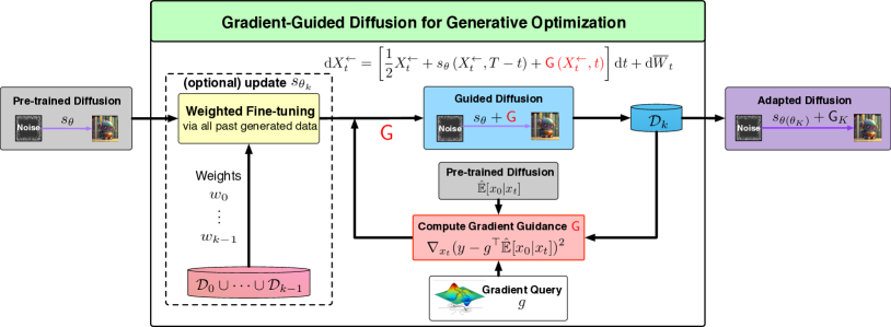
Figure 1: Gradient-guided diffusion model for generative optimization, with or without adaptive finetuning. A pre-trained diffusion model is guided with an additional gradient signal from an external objectives function towards generating near-optimal solutions.

Scope of This Paper

We investigate the role of guidance in diffusion models from an optimization perspective. The goal is to generate samples that optimize a given objective function f𝑓f. Drawing inspiration from gradient-based optimization methods, we construct a guidance signal based on the gradient vector, f𝑓\nabla f. Then we use the gradient signal, in addition to the pre-trained score function, to guide the sampling process towards generating structured output with higher function values. See Figure 1 for illustration our algorithmic framework. Our main results are summarized as follows:

  • We focus on structured data. Assume that pre-trained data belongs to a latent low-dimensional subspace, thus the trained score function is capable of discerning and maintaining the latent subspace structure of data during (unguided) generation. To guide the generation, we introduce a gradient-like guidance based on a forward prediction loss (Definition 1). This gradient guidance can be computed based on a pre-trained score network, and it provably preserve any learned low-dimensional structure in the generated output (Lemma 1).

  • We formalize a mathematical framework of using a gradient-guided diffusion model for generative optimization. While retaining the pre-trained score function, the generation process is iteratively refined and guided using new gradient queries (Algorithm 1; Figure 1 without fine-tuning). Under proper assumptions, we demonstrate that this adapted model generates novel samples whose expectation converges to a solution that is regularized with respect to the original problem (Theorem 2). The regularization ensures that the generated samples remain proximal to the training data. In other words, gradient guidance cannot shift data distribution unboundedly towards higher objective values, revealing a fundamental limit for adapting pre-trained diffusion models.

  • Furthermore, we explore an adaptive variant of gradient-guided diffusion, where both the score function and gradient guidance are iteratively fine-tuned using self-generated samples (Algorithm 2; Figure 1 with fine-tuning). Although slightly increasing the computational demand, we provide evidence that this approach generates new samples whose expectation converges to global optima, within the latent subspace, at a rate of 𝒪(1/K)𝒪1𝐾\mathcal{O}(1/K) (Theorems 3 and 4), where K𝐾K denotes the number of iterations and gradient evaluations, matching classical convergence theory of convex optimization.

Our findings suggest that this novel gradient guidance not only preserves the latent subspace structure of the data but also ensures fast convergence towards the optimal solution. Numerical experiments with a pre-trained U-network score function are provided in Section 7 to support these theoretical findings.

2 Related Work

Our study is motivated by recent empirical progress of guidance-based diffusion model fine-tuning for steering sample generation towards specific needs (Dhariwal and Nichol, 2021; Bansal et al., 2023). Upon modeling the specific needs as a reward function, the relevant methods can be summarized into two categories in the sequel.

Guided Generation and Fine-tuning

Given an auxiliary reward function judging the sample property of interests, existing research explored diverse mechanisms to guide generation from diffusion models. There are mainly two types of methods. The first type of method incorporates an additive so-called “guidance” term into the score function of pre-trained diffusion models at inference time. For example, classifier guidance (Song et al., 2020a; Dhariwal and Nichol, 2021) defines the guidance term as the gradient of an externally trained classifier on noise corrupted data. Classifier-free guidance (Ho and Salimans, 2022) simultaneously trains conditional and unconditional diffusion models, circumventing the training of an external classifier. After the training, the score functions of the conditional and unconditional models are combined together to achieve guided generation. Bansal et al. (2023) draw motivation from classifier guidance and generalize the idea to a “universal guidance” for adapting unconditioned score functions to various external rewards.

The second type of method attempts to directly fine-tune the weight parameters in a pre-trained diffusion model by interacting with the target reward function. For example, Clark et al. (2023) fine-tune diffusion models by directly backpropagating the gradient of the reward function. Recently, a line of works utilizes Reinforcement Learning (RL) techniques for fine-tuning diffusion models (Black et al., 2023; Fan et al., 2023). They formulate the sample generation process of diffusion models as a finite-horizon Markov chain. The score function can be viewed as a policy, the generated samples are the state of the Markov chain, and the target reward function defines the terminal reward. In this way, fine-tuning diffusion models is equivalent to policy optimization and allows the use of policy gradient methods.

Sampling and Statistical Theory of Diffusion Model

In contrast to the fruitful empirical advances, the theory of diffusion models is still limited. To the best of our knowledge, a theoretical understanding of fine-tuning diffusion models is absent. Existing results mainly focus on the sampling ability and statistical properties of unconditional diffusion models. In particular, for sampling ability, a line of works shows that the distribution generated by a diffusion model is close to the data distribution, as long as the score function is accurately estimated (De Bortoli et al., 2021; Albergo et al., 2023; Block et al., 2020; Lee et al., 2022a; Chen et al., 2022; Lee et al., 2022b, a; Chen et al., 2022; Lee et al., 2022b). The accuracy of the estimated score function is measured in terms of an Lsubscript𝐿L_{\infty} or L2subscript𝐿2L_{2}-norm distance. More recently, Chen et al. (2023c, b); Benton et al. (2023) develop refined and tighter analyses using Taylor expansions of the discretized backward process and localization method. It is worth mentioning that the analysis in Chen et al. (2023c, b); Benton et al. (2023) extends to broader sample generation processes such as deterministic ones based on probabilistic ODEs. Going beyond distributions in Euclidean spaces, De Bortoli (2022) analyzes diffusion models for sampling distribution supported on a low-dimensional manifold. Moreover, Montanari and Wu (2023) consider sampling from symmetric spiked models, and El Alaoui et al. (2023) study sampling from Gibbs distributions using diffusion processes.

Turning towards the statistical theory of diffusion models, Song et al. (2020b) and Liu et al. (2022) provide asymptotic analyses, assuming a parametric form of the score function. Unfortunately, asymptotic analysis does not lead to concrete sample complexities. Later, concurrent works, Oko et al. (2023) and Chen et al. (2023a), establish sample complexity bounds of diffusion models for estimating nonparametric data distributions. In high dimensions, their results highlight a curse of dimensionality issue without further assumptions, which also appears in Wibisono et al. (2024) considering kernel methods. More interestingly, these works demonstrate that diffusion models can circumvent the curse of dimensionality issue if the data has low-dimensional structures. In the same spirit, Mei and Wu (2023) investigate learning high-dimensional graphical models using diffusion models, without the curse of dimensionality. For conditional diffusion models, Yuan et al. (2023); Fu et al. (2024) establish sample complexity bounds for learning generic conditional distributions. We refer readers to Chen et al. (2024) for an overview of contemporary theoretical progress.

Novelty of This Paper

Despite the existing theoretical underpinnings of diffusion models, our paper provides the first rigorous study of adapting and fine-tuning diffusion models using gradient guidance from an optimization perspective. Specifically, we first understand why naive gradient guidance does not lead to meaningful optimization performance. Built upon the insights gained from the analysis, we propose gradient guidance that is proven to preserve generated data structures and simultaneously achieve strong optimization guarantees on adapted variants of diffusion models.

We are aware of two recent works (Uehara et al., 2024; Marion et al., 2024) studying adapting the output distribution of diffusion models to a target reward function. In particular, they define a reward function with respect to the output distribution of the diffusion model. Given a pre-trained diffusion model, for instance, Uehara et al. (2024) utilizes a KL-divergence regularizer penalizing the deviation to the pre-trained model for preventing overfitting in fine-tuning. Through some explicit computation, Uehara et al. (2024); Marion et al. (2024) identify the proper guidance term to adapt the pre-trained model. Yet a sophisticated estimation procedure is needed to find the guidance term in Uehara et al. (2024); our gradient guidance enjoys much simplicity and efficacy, as we demonstrated in both theory and experiments.

3 Preliminaries: Diffusion Models

Score-based diffusion models capture the distribution of pre-training data by learning a sequence of transformations to generate new samples from noise (Song et al., 2020c). A forward stochastic process progressively adds noise to data, whose sample trajectories are used to train the score function. To generate new samples, a backward denoising process starts from sampling pure noise and gradually transforms the noise guided by the learned score function.

Forward Process

The forward process of diffusion models initializes with X0Dsubscript𝑋0superscript𝐷X_{0}\in\mathbb{R}^{D}, a random variable drawn from the pre-training data 𝒟𝒟\mathcal{D}. It introduces noise to via an Ornstein-Uhlenbeck process, i.e.,

dXt=12q(t)Xtdt+q(t)dWtforq(t)>0,dsubscript𝑋𝑡12𝑞𝑡subscript𝑋𝑡d𝑡𝑞𝑡dsubscript𝑊𝑡for𝑞𝑡0\mathop{}\!\mathrm{d}X_{t}=-\frac{1}{2}q(t)X_{t}\mathop{}\!\mathrm{d}t+\sqrt{q(t)}\mathop{}\!\mathrm{d}W_{t}~{}~{}~{}\text{for}~{}~{}q(t)>0, (1)

where (Wt)t0subscriptsubscript𝑊𝑡𝑡0(W_{t})_{t\geq 0} is a standard Wiener process, and q(t)𝑞𝑡q(t) is a non-decreasing weighting function. Xtsubscript𝑋𝑡X_{t} represents the noise-corrupted data distribution at time t𝑡t. Given X0=x0subscript𝑋0subscript𝑥0X_{0}=x_{0}, the conditional distribution Xt|X0=x0conditionalsubscript𝑋𝑡subscript𝑋0subscript𝑥0X_{t}|X_{0}=x_{0} is Gaussian, i.e., 𝒩(α(t)x0,h(t)ID)𝒩𝛼𝑡subscript𝑥0𝑡subscript𝐼𝐷\mathcal{N}(\alpha(t)x_{0},h(t)I_{D}) with α(t)=exp(0t12q(s)𝑑s)𝛼𝑡superscriptsubscript0𝑡12𝑞𝑠differential-d𝑠\alpha(t)=\exp(-\int_{0}^{t}\frac{1}{2}q(s)ds) and h(t)=1α2(t)𝑡1superscript𝛼2𝑡h(t)=1-\alpha^{2}(t). In practice, the forward process will terminate at a large time T𝑇T so that the marginal distribution of XTsubscript𝑋𝑇X_{T} is close to 𝒩(0,ID)𝒩0subscript𝐼𝐷\mathcal{N}(0,I_{D}). In our analysis, we take q(t)1𝑞𝑡1q(t)\equiv 1 without loss of generality, where α(t):=exp(t/2)assign𝛼𝑡𝑡2\alpha(t):=\exp(-t/2) and h(t):=1exp(t)assign𝑡1𝑡h(t):=1-\exp(-t).

Backward Process

If reversing the time of the forward process, we can reconstruct the original distribution of the data from pure noise. With (W¯t)t0subscriptsubscript¯𝑊𝑡𝑡0(\overline{W}_{t})_{t\geq 0} being another independent Wiener process, the backward SDE below (Anderson, 1982) reverses the time in the forward SDE (1),

dXt=[12Xt+logpTt(Xt)score]dt+dW¯t.dsubscriptsuperscript𝑋𝑡delimited-[]12subscriptsuperscript𝑋𝑡subscriptsubscript𝑝𝑇𝑡subscriptsuperscript𝑋𝑡scored𝑡dsubscript¯𝑊𝑡\mathop{}\!\mathrm{d}X^{\leftarrow}_{t}=\left[\frac{1}{2}X^{\leftarrow}_{t}+{\underbrace{\nabla\log p_{T-t}(X^{\leftarrow}_{t})}_{\text{score}}}\right]\mathop{}\!\mathrm{d}t+\mathop{}\!\mathrm{d}\overline{W}_{t}. (2)

Here pt()subscript𝑝𝑡p_{t}(\cdot) denotes the marginal density of Xtsubscript𝑋𝑡X_{t} in the forward process. In the forward SDE (2), the score function logpt()subscript𝑝𝑡\nabla\log p_{t}(\cdot) plays a crucial role, but it has to be estimated from data.

Score Matching

To learn the unknown score function logpt()subscript𝑝𝑡\nabla\log p_{t}(\cdot), it is common to train a score network sθ(x,t)subscript𝑠𝜃𝑥𝑡s_{\theta}(x,t) using samples generated by the forward process. Let 𝒟𝒟\mathcal{D} denote the data for training. Then the score network is learned by minimizing the following loss:

mins𝒮0T𝔼x0𝒟𝔼xt|x0[xtlogϕt(xt|x0)s(xt,t)2]dt,\displaystyle\hbox{min}_{s\in\mathcal{S}}\int_{0}^{T}{\mathbb{E}}_{x_{0}\in\mathcal{D}}\mathbb{E}_{x_{t}|x_{0}}\left[\left\lVert\nabla_{x_{t}}\log\phi_{t}(x_{t}|x_{0})-s(x_{t},t)\right\lVert^{2}\right]\mathop{}\!\mathrm{d}t, (3)

where 𝒮𝒮{\mathcal{S}} is a given function class, 𝔼𝒟subscript𝔼𝒟{\mathbb{E}}_{\mathcal{D}} denotes the empirical expectation over training data 𝒟𝒟\mathcal{D} and 𝔼xt|x0subscript𝔼conditionalsubscript𝑥𝑡subscript𝑥0\mathbb{E}_{x_{t}|x_{0}} denotes condition expectation over the forward process, ϕt(xt|x0)subscriptitalic-ϕ𝑡conditionalsubscript𝑥𝑡subscript𝑥0\phi_{t}(x_{t}|x_{0}) is the Gaussian transition kernel, i.e., 1(2πh(t))D/2exp(xtα(t)x022h(t))1superscript2𝜋𝑡𝐷2superscriptdelimited-∥∥subscript𝑥𝑡𝛼𝑡subscript𝑥022𝑡\frac{1}{(2\pi h(t))^{D/2}}\exp(-\frac{\lVert x_{t}-\alpha(t)x_{0}\rVert^{2}}{2h(t)}).

Generation and Guided Generation

Given a pre-trained score function sθsubscript𝑠𝜃s_{\theta}, one generates new samples by simulating the backward process (2) with the true score replaced by sθsubscript𝑠𝜃s_{\theta}. Further, one can add additional guidance to the backward SDE to steer its output distribution towards specific properties of interest. Module 1 formalizes the generation process and guided generation process using a pre-trained diffusion model.

1:  Input: Score sθsubscript𝑠𝜃s_{\theta}, guidance G default to be zero for unguided generation.
2:  Hyper-parameter: T𝑇T.
3:  Initialized at Xt𝒩(0,I)similar-tosubscriptsuperscript𝑋𝑡𝒩0𝐼X^{\leftarrow}_{t}\sim\mathcal{N}(0,I), simulate the following SDE till time T𝑇T:
dXt=[12Xt+sθ(Xt,Tt)+G(Xt,Tt)]dt+dW¯t.dsubscriptsuperscript𝑋𝑡delimited-[]12subscriptsuperscript𝑋𝑡subscript𝑠𝜃subscriptsuperscript𝑋𝑡𝑇𝑡Gsubscriptsuperscript𝑋𝑡𝑇𝑡d𝑡dsubscript¯𝑊𝑡\mathop{}\!\mathrm{d}X^{\leftarrow}_{t}=\left[\frac{1}{2}X^{\leftarrow}_{t}+{s_{\theta}\left(X^{\leftarrow}_{t},T-t\right)+\texttt{G}\left(X^{\leftarrow}_{t},T-t\right)}\right]\mathop{}\!\mathrm{d}t+\mathop{}\!\mathrm{d}\overline{W}_{t}.
4:  Output: Sample XTsuperscriptsubscript𝑋𝑇X_{T}^{\leftarrow}.
Module 1 Guided_BackwardSample(sθ,G)Guided_BackwardSamplesubscript𝑠𝜃G\texttt{Guided\_BackwardSample}(s_{\theta},\texttt{G})

Conditional Generation

Suppose the goal is to generate X𝑋X with a desired property Y=y𝑌𝑦Y=y from the distribution P(X|Y=y)𝑃conditional𝑋𝑌𝑦P(X|Y=y). To this end, one needs the conditional score function xtlogpt(xty)subscriptsubscript𝑥𝑡subscript𝑝𝑡conditionalsubscript𝑥𝑡𝑦\nabla_{x_{t}}\log p_{t}(x_{t}\mid y), as a replacement of the unconditioned score xtlogpt(xt)subscriptsubscript𝑥𝑡subscript𝑝𝑡subscript𝑥𝑡\nabla_{x_{t}}\log p_{t}(x_{t}). The Bayes rule gives

xtlogpt(xty)=logpt(xt)est. by sθ(xt,t)+xtlogpt(yxt)to be est. by guidance.subscriptsubscript𝑥𝑡subscript𝑝𝑡conditionalsubscript𝑥𝑡𝑦subscriptsubscript𝑝𝑡subscript𝑥𝑡est. by subscript𝑠𝜃subscript𝑥𝑡𝑡subscriptsubscriptsubscript𝑥𝑡subscript𝑝𝑡conditional𝑦subscript𝑥𝑡to be est. by guidance\nabla_{x_{t}}\log p_{t}(x_{t}\mid y)=\underbrace{\nabla\log p_{t}(x_{t})}_{\text{est. by }s_{\theta}(x_{t},t)}+\underbrace{\nabla_{x_{t}}\log p_{t}(y\mid x_{t})}_{\text{to be est. by guidance}}. (4)

When a pre-trained score network sθ(xt,t)logpt(xt)subscript𝑠𝜃subscript𝑥𝑡𝑡subscript𝑝𝑡subscript𝑥𝑡s_{\theta}(x_{t},t)\approx\nabla\log p_{t}(x_{t}), the remaining task is to estimate xtlogpt(yxt)subscriptsubscript𝑥𝑡subscript𝑝𝑡conditional𝑦subscript𝑥𝑡\nabla_{x_{t}}\log p_{t}(y\mid x_{t}) and add it as a “guidance” G to the backward process (Module 1).

Classifier and Classifier-Free Guidance

Classifier guidance (Song et al., 2020c; Dhariwal and Nichol, 2021) is a approach for sampling from P(X|Y=y)𝑃conditional𝑋𝑌𝑦P(X|Y=y) when Y𝑌Y is a discrete label. This method estimates xtlogpt(yxt)subscriptsubscript𝑥𝑡subscript𝑝𝑡conditional𝑦subscript𝑥𝑡\nabla_{x_{t}}\log p_{t}(y\mid x_{t}) by training auxiliary classifiers, denoted as p^(yxt,t)^𝑝conditional𝑦subscript𝑥𝑡𝑡\hat{p}(y\mid x_{t},t), and then computing the gradient of the classifier logits as the guidance, i.e., G(xt,t)=xtlogp^(yxt,t)Gsubscript𝑥𝑡𝑡subscriptsubscript𝑥𝑡^𝑝conditional𝑦subscript𝑥𝑡𝑡\texttt{G}(x_{t},t)=\nabla_{x_{t}}\log\hat{p}(y\mid x_{t},t). An alternative is the classifier-free guidance method (Ho and Salimans, 2022), which jointly trains a conditional and an unconditional diffusion model, and combine the two score estimates via a form of guidance to generate samples.

Notations

For a random variable X𝑋X, Pxsubscript𝑃𝑥P_{x} represents its distribution, and p(x)𝑝𝑥p(x) denotes its density function. For X𝑋X, Y𝑌Y jointly distributed, P(XY=y)𝑃conditional𝑋𝑌𝑦P(X\mid Y=y) denotes the conditional distribution, and p(xy)𝑝conditional𝑥𝑦p(x\mid y) denotes its density function. We use the notation 𝔼[xy]𝔼delimited-[]conditional𝑥𝑦\mathbb{E}[x\mid y] for the conditional expectation. Let 𝒟𝒟\mathcal{D} be the pre-training data, and let 𝔼𝒟subscript𝔼𝒟{\mathbb{E}}_{\mathcal{D}} be the empirical expectation over 𝒟𝒟\mathcal{D}. Let μ¯¯𝜇\bar{\mu} and Σ¯¯Σ\bar{\Sigma} denote the data’s empirical mean and covariance matrix, i.e., μ¯:=𝔼x𝒟[x]assign¯𝜇subscript𝔼𝑥𝒟delimited-[]𝑥\bar{\mu}:={\mathbb{E}}_{x\in\mathcal{D}}[x] and Σ¯:=𝔼x𝒟[(xμ¯)(xμ¯)]assign¯Σsubscript𝔼𝑥𝒟delimited-[]𝑥¯𝜇superscript𝑥¯𝜇top\bar{\Sigma}:={\mathbb{E}}_{x\in\mathcal{D}}\left[(x-\bar{\mu})(x-\bar{\mu})^{\top}\right]. For a matrix A𝐴A, we denote by Span(A)Span𝐴\hbox{Span}(A) the subspace spanned by its column vectors. For a square matrix A𝐴A, we denote by A1superscript𝐴1A^{-1} its inverse or Moore–Penrose inverse. For any differentiable function f:nm:𝑓superscript𝑛superscript𝑚f:\mathbb{R}^{n}\to\mathbb{R}^{m}, fm×n𝑓superscript𝑚𝑛\nabla f\in\mathbb{R}^{m\times n} denotes Jacobian matrix, i.e., (f)ij=fi(x)xj.subscript𝑓𝑖𝑗subscript𝑓𝑖𝑥subscript𝑥𝑗(\nabla f)_{ij}=\frac{\partial f_{i}(x)}{\partial x_{j}}.

4 A Primer on Gradient Guidance

Suppose we have a pre-trained diffusion model where the score network sθ(xt,t)subscript𝑠𝜃subscript𝑥𝑡𝑡s_{\theta}(x_{t},t) provides a good approximation to the true score function logp(xt)𝑝subscript𝑥𝑡\log p(x_{t}). Then this diffusion model is viewed as an implicit density estimator of the pre-training data’s distribution. Its backward process (2) generates samples from this estimated distribution (Oko et al., 2023; Chen et al., 2023a).

Now suppose we want to generate novel samples with desired properties that can be measured by a differentiable function f𝑓f. We will refer to f𝑓f as a reward or objective function later on, and it is often user-specified. Motivated by the gradient methodology in optimization, a natural, intuitive way for adding guidance is to steer the generated samples towards the steepest ascent direction of f𝑓f (Bansal et al., 2023; Clark et al., 2023). This motivates the following guided backward process (Module 1):

dXt=[12Xt+sθ(Xt,Tt)+G(Xt,t)]dt+dW¯t.dsubscriptsuperscript𝑋𝑡delimited-[]12subscriptsuperscript𝑋𝑡subscript𝑠𝜃subscriptsuperscript𝑋𝑡𝑇𝑡Gsuperscriptsubscript𝑋𝑡𝑡d𝑡dsubscript¯𝑊𝑡\displaystyle\mathop{}\!\mathrm{d}X^{\leftarrow}_{t}=\left[\frac{1}{2}X^{\leftarrow}_{t}+s_{\theta}(X^{\leftarrow}_{t},T-t){\color[rgb]{1,0,0}+{\texttt{G}}(X_{t}^{\leftarrow},t)}\right]\mathop{}\!\mathrm{d}t+\mathop{}\!\mathrm{d}\overline{W}_{t}.

Here the guidance term G is what we focus on and wish to design. Specifically, we want to construct this guidance term G based on the gradient f𝑓\nabla f of a general objective f𝑓f.

4.1 Subspace Data and Score Decomposition

Real-world data often has rich intrinsic structures. These structures can be induced by local regularities, global symmetries, and repetitive patterns (Tenenbaum et al., 2000; Roweis and Saul, 2000) and are often low-dimensional (Pope et al., 2021). The power of diffusion models is to model the latent distribution and generate novel samples that preserve important characteristics of real-world data. If we blindly improve f𝑓f at the cost of losing these characteristics, the quality of new samples would degrade dramatically. This quality degradation, also known as “reward over-optimization”, is a common challenge for adapting diffusion models towards an external reward (Yuan et al., 2023; Uehara et al., 2024).

We aim to design gradient guidance to improve objective function while mitigating the risk of over-optimization. To this end, we focus on data that admits a low-dimensional latent subspace. Let us make the following assumption.

Assumption 1 (Subspace Data).

Data XD𝑋superscript𝐷X\in\mathbb{R}^{D} can be represented as X=AU𝑋𝐴𝑈X=AU, where AD×d𝐴superscript𝐷𝑑A\in\mathbb{R}^{D\times d} is an unknown matrix and the latent variable Ud𝑈superscript𝑑U\in\mathbb{R}^{d} follows some distribution Pusubscript𝑃𝑢P_{u} with a density pusubscript𝑝𝑢p_{u}. Here dDmuch-less-than𝑑𝐷d\ll D. We assume the empirical covariance of U𝑈U is full rank.

Under 1, the score function logpt(x)subscript𝑝𝑡𝑥\nabla\log p_{t}(x) decomposes to two orthogonal parts: an on-support component belonging to the subspace; and an orthogonal component. We recall this key result in Proposition 1.

Proposition 1 (Score Decomposition for Subspace Data (Chen et al. (2023a) Lem. 1, Thm. 3)).

Under 1, the score function logpt(x)subscript𝑝𝑡𝑥\nabla\log p_{t}(x) decomposes as

logpt(x)=Alogpt𝖫𝖣(Ax)𝐬(Ax,t): on-support score1h(t)(IDAA)x𝐬(x,t): ortho. score.subscript𝑝𝑡𝑥subscript𝐴superscriptsubscript𝑝𝑡𝖫𝖣superscript𝐴top𝑥subscript𝐬parallel-tosuperscript𝐴top𝑥𝑡: on-support scoresubscript1𝑡subscript𝐼𝐷𝐴superscript𝐴top𝑥subscript𝐬perpendicular-to𝑥𝑡: ortho. score\displaystyle\nabla\log p_{t}(x)=\underbrace{A\nabla\log p_{t}^{\sf LD}(A^{\top}x)}_{\mathbf{s}_{\parallel}(A^{\top}x,t)\text{:~{}on-support~{}score}}-\underbrace{\frac{1}{h(t)}\left(I_{D}-AA^{\top}\right)x}_{\mathbf{s}_{\perp}(x,t)\text{:~{}ortho.~{}score}}. (5)

where pt𝖫𝖣(u)=ϕt(u|u)pu(u)dusuperscriptsubscript𝑝𝑡𝖫𝖣superscript𝑢subscriptitalic-ϕ𝑡conditionalsuperscript𝑢𝑢subscript𝑝𝑢𝑢differential-d𝑢p_{t}^{\sf LD}(u^{\prime})=\int\phi_{t}(u^{\prime}|u)p_{u}(u)\mathop{}\!\mathrm{d}u with ϕt(|u)\phi_{t}(\cdot|u) being the density of 𝒩(α(t)u,h(t)Id)𝒩𝛼𝑡𝑢𝑡subscript𝐼𝑑\mathcal{N}(\alpha(t)u,h(t)I_{d}) for the same α(t)𝛼𝑡\alpha(t) and h(t)𝑡h(t) in the forward process (1).

According to Chen et al. (2023a), pre-training a score function on subspace data takes advantage of the decomposition given by (5) and learns the latent subspace. When the pre-trained score network is used to generate new samples, the backward sampling process also decomposes into two orthogonal processes due to (5). Analysis of this backward process proves that the generated output would remain proximal to the latent subspace. This explains why diffusion models can learn and preserve data’s underlying characteristics. We refer interested readers to Chen et al. (2023a) for more discussions.

In the rest of this section, we investigate the principles for designing a guidance based on the gradient of f𝑓f that ensures generated samples (i) improve the value of f𝑓f, and at the same time, (ii) adhere to the subspace structure, i.e. generated samples being close to the subspace spanned by A𝐴A.

4.2 Naive Gradient Does’t Work as Guidance

Motivated by the gradient optimization methodology, a natural, intuitive way for adding guidance is to steer the generated samples towards the steepest ascent direction of f𝑓f (Bansal et al., 2023; Clark et al., 2023). Therefore, a tempting simple choice of the guidance G is the steepest ascent direction, which we refer to as naive gradient guidance i.e.,

G(Xt,t)f(Xt).proportional-toGsuperscriptsubscript𝑋𝑡𝑡𝑓superscriptsubscript𝑋𝑡{\texttt{G}}(X_{t}^{\leftarrow},t)\propto\nabla f(X_{t}^{\leftarrow}). (6)

This naive choice of guidance signal G would steer the movement of the original backward process towards the direction that increases f𝑓f.

However, the naive gradient guidance (6) is never adopted in practice; existing methods have to resort to more sophisticated forms of guidance or more computationally demanding fine-tuning methods; for example Bansal et al. (2023); Uehara et al. (2024); Marion et al. (2024). Introducing gradient information indiscriminately into the backward SDE has the risk of potentially leading the stochastic denoising process to divergence, and compromising the data structures learned during pre-training.
Refer to caption
Refer to caption
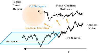
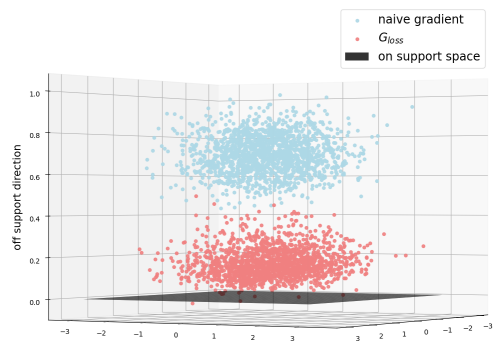
Figure 2: Directly adding the gradient of the objective function to the backward sampling process sabotages the subspace structure. Left: When gradients are pointing out of the data subspace, adding them directly to the backward SDE will make samples go off the subspace. Right: Numerical experiments show that naive gradients lead to substantially larger off-subspace error compared to our gradient guidance GlosssubscriptG𝑙𝑜𝑠𝑠\texttt{G}_{loss}(Definition 1); see Section 7 for experiment details.

Let us suppose the data distribution is supported on a low-dimensional subspace as in Assumption 1. We explain why naive gradients do not work as guidance. With subspace data, the score function would steer the distribution towards concentrating onto the latent subspace, due to its special decomposition form given by Proposition 1. We refer interested readers to Chen et al. (2023a) for detailed analysis of this phenomenon.

However, naive gradient vectors can be pointing towards any direction, not limited to within the latent subspace. Thus directly adding gradient guidance to the backward process could jeopardize the decomposition form of the score function, and it would also jeopardize the latent structure in the generated output. See Figure 2 for illustration and experiment results. The failure of naive gradient motivates us to seek robust alternatives.

4.3 Motivating Gradient Guidance from Conditional Score Function

We want to study how to add guidance to the sampling process utilizing the gradient of f𝑓f. To motivate our design of guidance, we start with the most elementary Gaussian probabilistic model. Later we will drop this assumption and consider general data distributions and general f𝑓f.

Assumption 2 (Gaussian model).

Let data follow a Gaussian distribution, i.e., X𝒩(μ,Σ)similar-to𝑋𝒩𝜇ΣX\sim\mathcal{N}(\mu,\Sigma), and let f(x)=gx𝑓𝑥superscript𝑔top𝑥f(x)=g^{\top}x be a linear function for some gD𝑔superscript𝐷g\in\mathbb{R}^{D}. Let Y=f(X)+ϵ𝑌𝑓𝑋italic-ϵY=f(X)+\epsilon with independent, identically distributed noise ϵ𝒩(0,σ2)similar-toitalic-ϵ𝒩0superscript𝜎2\epsilon\sim\mathcal{N}(0,\sigma^{2}) for some σ>0𝜎0\sigma>0.

To generate samples from P(X|Y=y)𝑃conditional𝑋𝑌𝑦P(X|Y=y), we need to train a diffusion model with a conditional score function. By the Bayes’ rule, the conditional score function takes the form of a sum given by

xtlogpt(xty)=logpt(xt)est. by sθ(xt,t)+xtlogpt(yxt)to be est. by guidance.subscriptsubscript𝑥𝑡subscript𝑝𝑡conditionalsubscript𝑥𝑡𝑦subscriptsubscript𝑝𝑡subscript𝑥𝑡est. by subscript𝑠𝜃subscript𝑥𝑡𝑡subscriptsubscriptsubscript𝑥𝑡subscript𝑝𝑡conditional𝑦subscript𝑥𝑡to be est. by guidance\nabla_{x_{t}}\log p_{t}(x_{t}\mid y)=\underbrace{\nabla\log p_{t}(x_{t})}_{\text{est. by }s_{\theta}(x_{t},t)}+\underbrace{\nabla_{x_{t}}\log p_{t}(y\mid x_{t})}_{\text{to be est. by guidance}}. (recall (4))

Now if we already have a pre-trained score function sθsubscript𝑠𝜃s_{\theta}, the remaining task is to estimate the second term logpt(yxt)subscript𝑝𝑡conditional𝑦subscript𝑥𝑡\log p_{t}(y\mid x_{t}). Under the Gaussian assumption, we derive the following closed-form conditional score. The proof is provided in Appendix B.1.

Lemma 1 (Conditional score gives a gradient-like guidance).

Under Assumption 2, we have

xtlogpt(y|xt)=β(t)[yg𝔼[x0|xt]](α2(t)Σ+h(t)ID)1Σg,subscriptsubscript𝑥𝑡subscript𝑝𝑡conditional𝑦subscript𝑥𝑡𝛽𝑡delimited-[]𝑦superscript𝑔top𝔼delimited-[]conditionalsubscript𝑥0subscript𝑥𝑡superscriptsuperscript𝛼2𝑡Σ𝑡subscript𝐼𝐷1Σ𝑔\nabla_{x_{t}}\log p_{t}(y|x_{t})=\beta(t)\left[y-g^{\top}\mathbb{E}[x_{0}|x_{t}]\right]\cdot\left(\alpha^{2}(t)\Sigma+h(t)I_{D}\right)^{-1}\Sigma g, (7)

where 𝔼[x0|xt]𝔼delimited-[]conditionalsubscript𝑥0subscript𝑥𝑡\mathbb{E}[x_{0}|x_{t}] denotes the conditional expectation of x0subscript𝑥0x_{0} given xtsubscript𝑥𝑡x_{t} in the forward process (1), α(t)=et/2𝛼𝑡superscript𝑒𝑡2\alpha(t)=e^{-t/2}, h(t)=1et𝑡1superscript𝑒𝑡h(t)=1-e^{-t} as in (1), and β(t)=α(t)/(σ2+gΣ1(ID+α2(t)/h(t)Σ)1g)𝛽𝑡𝛼𝑡superscript𝜎2superscript𝑔topsuperscriptΣ1superscriptsubscript𝐼𝐷superscript𝛼2𝑡𝑡Σ1𝑔\beta(t)=\alpha(t)/(\sigma^{2}+g^{\top}\Sigma^{-1}\left(I_{D}+\alpha^{2}(t)/h(t)\cdot\Sigma\right)^{-1}g).

Observe that, when Σ=IΣ𝐼\Sigma=I, (7) suggests the following form of guidance that is aligned with the naive gradient, i.e., the steepest ascent direction:

G(xt,t)[yg𝔼[x0|xt]]g.proportional-toGsubscript𝑥𝑡𝑡delimited-[]𝑦superscript𝑔top𝔼delimited-[]conditionalsubscript𝑥0subscript𝑥𝑡𝑔\texttt{G}(x_{t},t)\propto\left[y-g^{\top}\mathbb{E}[x_{0}|x_{t}]\right]\cdot g.

However, even for Gaussian distributions, as long as ΣIΣ𝐼\Sigma\neq I, the term of (7) is no longer proportional to g𝑔g but becomes a pre-conditioned version of the gradient.
Refer to caption
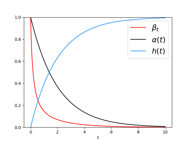
Figure 3: Plot of β(t),α(t),h(t)𝛽𝑡𝛼𝑡𝑡\beta(t),\alpha(t),h(t) for t[0,10]𝑡010t\in[0,10] when Σ=IΣ𝐼\Sigma=I.

Another observation is that this guidance scales with a residual term yg𝔼[x0xt]𝑦superscript𝑔top𝔼delimited-[]conditionalsubscript𝑥0subscript𝑥𝑡y-g^{\top}\mathbb{E}[x_{0}\mid x_{t}]. In particular, the residual term yg𝔼[x0xt]𝑦superscript𝑔top𝔼delimited-[]conditionalsubscript𝑥0subscript𝑥𝑡y-g^{\top}\mathbb{E}[x_{0}\mid x_{t}] tunes the strength of guidance. Recall 𝔼[x0xt]𝔼delimited-[]conditionalsubscript𝑥0subscript𝑥𝑡\mathbb{E}[x_{0}\mid x_{t}] denotes the posterior expectation of clean data x0subscript𝑥0x_{0} given xtsubscript𝑥𝑡x_{t} in the forward process. Thus, in a backward view, 𝔼[x0xt]𝔼delimited-[]conditionalsubscript𝑥0subscript𝑥𝑡\mathbb{E}[x_{0}\mid x_{t}] coincides with the expected sample to be generated conditioned on xtsubscript𝑥𝑡x_{t}. In this sense, the quantity yg𝔼[x0xt]𝑦superscript𝑔top𝔼delimited-[]conditionalsubscript𝑥0subscript𝑥𝑡y-g^{\top}\mathbb{E}[x_{0}\mid x_{t}] measures a look-ahead gap between the expected reward of generated samples and the target value. A larger absolute value of the residual means stronger guidance in the backward generation process.

We plot the theoretical choice of β(t)𝛽𝑡\beta(t) and α(t),h(t)𝛼𝑡𝑡\alpha(t),h(t) to t𝑡t in Figure 3. In practice, the choice of α(t),h(t)𝛼𝑡𝑡\alpha(t),h(t) can vary and they are determined by the forward process used for pre-training; and β(t)𝛽𝑡\beta(t) can be treated as a tuning parameter to adjust the strength of guidance.

4.4 Construct Gradient Guidance to Preserve Latent Subspace

When the data distribution is supported on a latent subspace, directly adding gradient guidance to the backward sampling process could jeopardize the data’s latent structure. We saw that this would lead to over-optimization, as illustrated in Figure 2.

To remedy such an issue, we propose the following modification to the gradient guidance. This modified gradient guidance takes advantage of a given score function.

Definition 1 (Gradient Guidance of Look-Ahead Loss).

Given a gradient vector g𝑔g, define the gradient guidance of look-ahead loss as

Gloss(xt,t):=β(t)xt(yg𝔼[x0|xt])2,\texttt{G}_{loss}(x_{t},t):=-\beta(t)\cdot\nabla_{x_{t}}\left(y-g^{\top}\mathbb{E}[x_{0}|x_{t}]\right)^{2}, (8)

where β(t)>0,yformulae-sequence𝛽𝑡0𝑦\beta(t)>0,y\in\mathbb{R} are tuning parameters, and 𝔼[x0|xt]𝔼delimited-[]conditionalsubscript𝑥0subscript𝑥𝑡\mathbb{E}[x_{0}|x_{t}] is the conditional expectation of x0subscript𝑥0x_{0} given xtsubscript𝑥𝑡x_{t} in the forward process (1), i.e., dXt=12q(t)Xtdt+q(t)dWt.dsubscript𝑋𝑡12𝑞𝑡subscript𝑋𝑡d𝑡𝑞𝑡dsubscript𝑊𝑡\mathop{}\!\mathrm{d}X_{t}=-\frac{1}{2}q(t)X_{t}\mathop{}\!\mathrm{d}t+\sqrt{q(t)}\mathop{}\!\mathrm{d}W_{t}.

The formula of (8) generalizes the intuition of a conditional score to work with any data distribution and objective function. The look-ahead loss (yg𝔼[x0|xt])2superscript𝑦superscript𝑔top𝔼delimited-[]conditionalsubscript𝑥0subscript𝑥𝑡2(y-g^{\top}\mathbb{E}[x_{0}|x_{t}])^{2} resembles the proximal term commonly used in first-order proximal optimization methods. It is worth noting that GlosssubscriptG𝑙𝑜𝑠𝑠\texttt{G}_{loss} coincides with the forward universal guidance xt(y,f(𝔼^[x0|xt]))subscriptsubscript𝑥𝑡𝑦𝑓^𝔼delimited-[]conditionalsubscript𝑥0subscript𝑥𝑡\nabla_{x_{t}}\ell(y,f(\hat{\mathbb{E}}[x_{0}|x_{t}])) proposed by Bansal et al. (2023) ((8) in their paper) when \ell is the square loss and f=gx𝑓superscript𝑔top𝑥f=g^{\top}x.

When the pre-training data distribution is Gaussian, the gradient guidance (8) is equivalent to Lemma 1 equation (7). This equivalence is a side-product from the proof of Lemma 1 and we provide a sketch here (see details in Section B.1). Given the probabilistic model 2, xtlogpt(y|xt)subscriptsubscript𝑥𝑡subscript𝑝𝑡conditional𝑦subscript𝑥𝑡\nabla_{x_{t}}\log p_{t}(y|x_{t}), the quantity to be estimated by guidance, is the score of a Gaussian distribution 𝒩(my(xt),σy2(xt))𝒩subscript𝑚𝑦subscript𝑥𝑡superscriptsubscript𝜎𝑦2subscript𝑥𝑡\mathcal{N}\left(m_{y}(x_{t}),\sigma_{y}^{2}(x_{t})\right), with my(xt)subscript𝑚𝑦subscript𝑥𝑡m_{y}(x_{t}) and σy2(xt)superscriptsubscript𝜎𝑦2subscript𝑥𝑡\sigma_{y}^{2}(x_{t}) being mean and variance of the conditional distribution YXt=xtconditional𝑌subscript𝑋𝑡subscript𝑥𝑡Y\mid X_{t}=x_{t} respectively, i.e.,

xtlogpt(yxt)=xt[12(ymy(xt)σy(xt))2]xtlogσy(xt),subscriptsubscript𝑥𝑡subscript𝑝𝑡conditional𝑦subscript𝑥𝑡subscriptsubscript𝑥𝑡12superscript𝑦subscript𝑚𝑦subscript𝑥𝑡subscript𝜎𝑦subscript𝑥𝑡2subscriptsubscript𝑥𝑡subscript𝜎𝑦subscript𝑥𝑡\nabla_{x_{t}}\log p_{t}(y\mid x_{t})=-\nabla_{x_{t}}\left[\displaystyle\frac{1}{2}\left(\frac{y-m_{y}(x_{t})}{\sigma_{y}(x_{t})}\right)^{2}\right]-\nabla_{x_{t}}\log\sigma_{y}(x_{t}), (9)

with my(xt)=g𝔼[x0xt]subscript𝑚𝑦subscript𝑥𝑡superscript𝑔top𝔼delimited-[]conditionalsubscript𝑥0subscript𝑥𝑡m_{y}(x_{t})=g^{\top}\mathbb{E}[x_{0}\mid x_{t}] and σy(xt)subscript𝜎𝑦subscript𝑥𝑡\sigma_{y}(x_{t}) not depending on xtsubscript𝑥𝑡x_{t}. Thus we see GlosssubscriptG𝑙𝑜𝑠𝑠\texttt{G}_{loss} is equivalent to (7).

A key advantage of GlosssubscriptG𝑙𝑜𝑠𝑠\texttt{G}_{loss} is that it enables preserving the subspace structure, for any data distribution under 1. This result is formally stated in the following theorem, we provide a proof sketch here and the full proof is in Section B.2.

Theorem 1 (Faithfulness of GlosssubscriptG𝑙𝑜𝑠𝑠\texttt{G}_{loss} to the Low-Dimensional Subspace of Data).

Under Assumption 1, it holds for any data distribution and gD𝑔superscript𝐷g\in\mathbb{R}^{D} that

Gloss(xt,t)Span(A).subscriptG𝑙𝑜𝑠𝑠subscript𝑥𝑡𝑡Span𝐴\texttt{G}_{loss}(x_{t},t)\in\operatorname{Span}(A). (10)

Proof Sketch

We have

xt(yg𝔼[x0|xt])2xt𝔼[x0|xt]g.\nabla_{x_{t}}\left(y-g^{\top}\mathbb{E}[x_{0}|x_{t}]\right)^{2}\propto\nabla_{x_{t}}\mathbb{E}[x_{0}|x_{t}]^{\top}g.

Note here that xt𝔼[x0|xt]subscriptsubscript𝑥𝑡𝔼delimited-[]conditionalsubscript𝑥0subscript𝑥𝑡\nabla_{x_{t}}\mathbb{E}[x_{0}|x_{t}] is the Jacobian matrix of 𝔼[x0|xt]𝔼delimited-[]conditionalsubscript𝑥0subscript𝑥𝑡\mathbb{E}[x_{0}|x_{t}], which is a mapping from Dsuperscript𝐷\mathbb{R}^{D} to Dsuperscript𝐷\mathbb{R}^{D}. We will show that the Jacobian xt𝔼[x0|xt]subscriptsubscript𝑥𝑡𝔼delimited-[]conditionalsubscript𝑥0subscript𝑥𝑡\nabla_{x_{t}}\mathbb{E}[x_{0}|x_{t}] maps any vector gD𝑔superscript𝐷g\in\mathbb{R}^{D} to Span(A)Span𝐴\hbox{Span}(A).

To see this, we utilize the score decomposition result of Proposition 1 which is

logpt(xt)=Alogpt𝖫𝖣(Axt)1h(t)(IDAA)xt.subscript𝑝𝑡subscript𝑥𝑡𝐴superscriptsubscript𝑝𝑡𝖫𝖣superscript𝐴topsubscript𝑥𝑡1𝑡subscript𝐼𝐷𝐴superscript𝐴topsubscript𝑥𝑡\nabla\log p_{t}(x_{t})=A\nabla\log p_{t}^{\sf LD}(A^{\top}x_{t})-\frac{1}{h(t)}\left(I_{D}-AA^{\top}\right)x_{t}. (recall (5))

Plugging (5) into the equality 𝔼[x0|xt]=1α(t)(xt+h(t)logpt(xt))𝔼delimited-[]conditionalsubscript𝑥0subscript𝑥𝑡1𝛼𝑡subscript𝑥𝑡𝑡subscript𝑝𝑡subscript𝑥𝑡{\mathbb{E}}[x_{0}|x_{t}]=\displaystyle\frac{1}{\alpha(t)}\left(x_{t}+h(t)\nabla\log p_{t}(x_{t})\right) (Tweedie’s formula (Efron, 2011)), we have

𝔼[x0|xt]=1α(t)(xt+h(t)[Am(Axt)1h(t)xt])=h(t)α(t)Am(Axt),𝔼delimited-[]conditionalsubscript𝑥0subscript𝑥𝑡1𝛼𝑡subscript𝑥𝑡𝑡delimited-[]𝐴𝑚superscript𝐴topsubscript𝑥𝑡1𝑡subscript𝑥𝑡𝑡𝛼𝑡𝐴𝑚superscript𝐴topsubscript𝑥𝑡\displaystyle{\mathbb{E}}[x_{0}|x_{t}]=\frac{1}{\alpha(t)}\left(x_{t}+h(t)\left[Am(A^{\top}x_{t})-\frac{1}{h(t)}x_{t}\right]\right)=\frac{h(t)}{\alpha(t)}Am(A^{\top}x_{t}), (11)

here we denote for short m(u):=logpt𝖫𝖣(u)+1h(t)uassign𝑚𝑢superscriptsubscript𝑝𝑡𝖫𝖣𝑢1𝑡𝑢m(u):=\nabla\log p_{t}^{\sf LD}(u)+\frac{1}{h(t)}u. From (11), we see that xt𝔼[x0|xt]subscriptsubscript𝑥𝑡𝔼superscriptdelimited-[]conditionalsubscript𝑥0subscript𝑥𝑡top\nabla_{x_{t}}\mathbb{E}[x_{0}|x_{t}]^{\top} maps any vector to Span(A)Span𝐴\operatorname{Span}(A) because m()𝑚m(\cdot) takes Axtsuperscript𝐴topsubscript𝑥𝑡A^{\top}x_{t} as input in the expression of 𝔼[x0|xt]𝔼delimited-[]conditionalsubscript𝑥0subscript𝑥𝑡{\mathbb{E}}[x_{0}|x_{t}]. \hfill\blacksquare

We highlight that the faithfulness of GlosssubscriptG𝑙𝑜𝑠𝑠\texttt{G}_{loss} holds for arbitrary data distribution supported on the latent subspace. It takes advantage of the score function’s decomposition (5), having the effect of automatically adapting g𝑔g onto the latent low-dimensional subspace of data.

4.5 Estimation and Implementation of GlosssubscriptG𝑙𝑜𝑠𝑠\texttt{G}_{loss}

Theorem 1 asserts that the gradient guidance given by Definition 1 provably preserves the subspace structure of data. However, GlosssubscriptG𝑙𝑜𝑠𝑠\texttt{G}_{loss} is not immediately available to compute and it involves the unknown quantity 𝔼[x0|xt]𝔼delimited-[]conditionalsubscript𝑥0subscript𝑥𝑡\mathbb{E}[x_{0}|x_{t}]. Next, we discuss the estimation and computation of GlosssubscriptG𝑙𝑜𝑠𝑠\texttt{G}_{loss} based on a pre-trained score function sθsubscript𝑠𝜃s_{\theta} in practice.

First, we need to estimate the quantity 𝔼[x0|xt]𝔼delimited-[]conditionalsubscript𝑥0subscript𝑥𝑡\mathbb{E}[x_{0}|x_{t}]. It is the conditional expectation of x0subscript𝑥0x_{0} given xtsubscript𝑥𝑡x_{t} in the forward process, thus it depends on the pre-training data distribution. One can construct estimate 𝔼[x0|xt]𝔼delimited-[]conditionalsubscript𝑥0subscript𝑥𝑡\mathbb{E}[x_{0}|x_{t}] based on the pre-trained score network sθsubscript𝑠𝜃s_{\theta}, by using the Tweedie’s formula (Efron, 2011):

logpt(xt)=𝔼[xtα(t)x0h(t)|xt].subscript𝑝𝑡subscript𝑥𝑡𝔼delimited-[]conditionalsubscript𝑥𝑡𝛼𝑡subscript𝑥0𝑡subscript𝑥𝑡\nabla\log p_{t}(x_{t})=-\mathbb{E}\left[\frac{x_{t}-\alpha(t)x_{0}}{h(t)}\big{|}x_{t}\right]. (12)

Suppose we have a given pre-trained score network that approximates the ground truth, i.e., sθ(xt,t)logpt(xt)subscript𝑠𝜃subscript𝑥𝑡𝑡subscript𝑝𝑡subscript𝑥𝑡s_{\theta}(x_{t},t)\approx\nabla\log p_{t}(x_{t}). Then a natural estimator of 𝔼^[x0|xt]^𝔼delimited-[]conditionalsubscript𝑥0subscript𝑥𝑡\hat{\mathbb{E}}[x_{0}|x_{t}] is given by

𝔼^[x0|xt]:=1α(t)(xt+h(t)sθ(xt,t)),assign^𝔼delimited-[]conditionalsubscript𝑥0subscript𝑥𝑡1𝛼𝑡subscript𝑥𝑡𝑡subscript𝑠𝜃subscript𝑥𝑡𝑡\hat{\mathbb{E}}[x_{0}|x_{t}]:=\displaystyle\frac{1}{\alpha(t)}\left(x_{t}+h(t){s}_{\theta}(x_{t},t)\right), (13)

and we refer to it as the look-ahead estimator. The estimator (13) is widely adopted in practice (Song et al., 2020a; Bansal et al., 2023). Here α(t)𝛼𝑡\alpha(t) and h(t)𝑡h(t) are the noise scheduling used in the forward process (1).

Thus, we have obtained an implementable version of the gradient guidance GlosssubscriptG𝑙𝑜𝑠𝑠\texttt{{G}}_{loss}, given by

Gloss(xt,t)=β(t)xt(yg(1α(t)(xt+h(t)sθ(xt,t))))2,\texttt{{G}}_{loss}(x_{t},t)=-\beta(t)\cdot\nabla_{x_{t}}\left(y-g^{\top}\left(\displaystyle\frac{1}{\alpha(t)}\left(x_{t}+h(t){s}_{\theta}(x_{t},t)\right)\right)\right)^{2}, (14)

With a slight abuse of notation, we use GlosssubscriptG𝑙𝑜𝑠𝑠\texttt{{G}}_{loss} to refer to this implementable formula (14) in the remainder of this paper.
Refer to caption
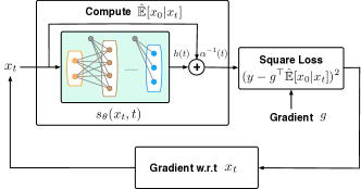
Figure 4: Computation of Gradient Guidance GlosssubscriptG𝑙𝑜𝑠𝑠\texttt{G}_{loss}.

The gradient guidance (14) has a light-weighted implementation. Suppose the pre-trained score function sθsubscript𝑠𝜃s_{\theta} is given in the form of a neural network with pre-trained weights. Computing (14) involves calculating the squared loss (yg𝔼^[x0|xt])2superscript𝑦superscript𝑔top^𝔼delimited-[]conditionalsubscript𝑥0subscript𝑥𝑡2\left(y-g^{\top}\hat{\mathbb{E}}[x_{0}|x_{t}]\right)^{2} via a forward pass of the network sθsubscript𝑠𝜃s_{\theta} and a backward pass utilizing the auto-gradient feature of deep-leaning frameworks such as PyTorch and TensorFlow. See Figure 4 for illustration.

Note that the value of y𝑦y in GlosssubscriptG𝑙𝑜𝑠𝑠\texttt{G}_{loss} is a target reward value, inherited from the conditional score analysis under a Gaussian model. In practice, we treat y𝑦y as a tuning parameter. In our theoretical analysis, we will specify the choices of y,β(t)𝑦𝛽𝑡y,\beta(t) and provide guarantees for general optimization beyond the Gaussian model.

So far, we have finally obtained a gradient guidance (14) that is both implementable and faithful to data’s latent subspace. The next step is to apply this gradient guidance and use it to adapt the generation process of a pre-trained diffusion model. Let us find out what one can obtain using gradient-guided diffusion models.

5 Gradient-Guided Diffusion Model as Regularized Optimizer

In this section, we study whether gradient guidance steers a pre-trained diffusion model to generate samples of near-optimal objective values. We provide a positive answer and our results are twofold: 1) We demonstrate that iteratively applying gradient guidance improves the generated samples towards higher objective values; 2) The pre-trained diffusion model acts as a form of regularization from an optimization perspective.

5.1 Gradient-Guided Generation with A Pre-trained Score

Assume access to a pre-trained score network sθsubscript𝑠𝜃s_{\theta} and gradient information of the objective function f𝑓f. Let us present our Algorithm 1 that adapts the pre-trained diffusion model and iteratively updates the gradient guidance (14). The gradient guidance is able to steer the backward sampling process towards generating new samples with higher values of f𝑓f. See Figure 1 for illustration.

Algorithm 1 takes as input any pre-trained score function sθ(x,t)subscript𝑠𝜃𝑥𝑡s_{\theta}(x,t) and adapts the backward sampling process with gradient guidance. In each iteration, it evaluates f()𝑓\nabla f(\cdot) at samples generated from the previous iteration (Line 5(i)), and then computes the gradient guidance GlosssubscriptG𝑙𝑜𝑠𝑠\texttt{G}_{loss} using the newly queried gradient (Line 5(ii)). Using the updated gradient guidance, the backward process then generate new samples with improved objective values (Module 1). At the end of iterations, the algorithm outputs an adapted version of the diffusion model, specified by (sθ,GK)subscript𝑠𝜃subscriptG𝐾(s_{\theta},\texttt{G}_{K}), which generates samples with near-optimal objective values.

1:  Input: Pre-trained score network sθ(,)subscript𝑠𝜃s_{\theta}(\cdot,\cdot), differentiable objective function f𝑓f.
2:  Tuning Parameter: Strength parameters β(t)𝛽𝑡\beta(t), {yk}k=0K1superscriptsubscriptsubscript𝑦𝑘𝑘0𝐾1\{y_{k}\}_{k=0}^{K-1}, number of iterations K𝐾K, batch sizes {Bk}subscript𝐵𝑘\{B_{k}\}.
3:  Initialization: G0=NULLsubscriptG0NULL\texttt{G}_{0}=\texttt{NULL}.
4:  for k=0,,K1𝑘0𝐾1k=0,\dots,K-1 do
5:     Generate: Sample zk,isimilar-tosubscript𝑧𝑘𝑖absentz_{k,i}\sim Guided_BackwardSample(sθ,Gk)Guided_BackwardSamplesubscript𝑠𝜃subscriptG𝑘\texttt{Guided\_BackwardSample}(s_{\theta},\texttt{G}_{k}) using Module 1, for i[Bk]𝑖delimited-[]subscript𝐵𝑘i\in[B_{k}].
6:     Compute Guidance: (i) Compute the sample mean z¯k:=(1/Bk)i=1Bkzk,iassignsubscript¯𝑧𝑘1subscript𝐵𝑘superscriptsubscript𝑖1subscript𝐵𝑘subscript𝑧𝑘𝑖\bar{z}_{k}:=(1/B_{k})\sum_{i=1}^{B_{k}}z_{k,i}.(ii) Query gradient gk=f(z¯k)subscript𝑔𝑘𝑓subscript¯𝑧𝑘g_{k}=\nabla f(\bar{z}_{k}).(iii) Update gradient guidance Gk+1(,)=Gloss(,)subscriptG𝑘1subscriptG𝑙𝑜𝑠𝑠\texttt{G}_{k+1}(\cdot,\cdot)=\texttt{G}_{loss}(\cdot,\cdot) via (8), using sθsubscript𝑠𝜃s_{\theta}, gradient vector gksubscript𝑔𝑘g_{k}, and parameters yksubscript𝑦𝑘y_{k} and β(t)𝛽𝑡\beta(t).
7:  end for
8:  Output: (sθ,GKsubscript𝑠𝜃subscriptG𝐾s_{\theta},\texttt{G}_{K}).
Algorithm 1 Gradient-Guided Diffusion for Generative Optimization

It is worth highlighting that Algorithm 1 works with any pre-trained score network sθ(xt,t)subscript𝑠𝜃subscript𝑥𝑡𝑡s_{\theta}(x_{t},t). It retains the original score network and only updates the guidance term. The gradient guidance changes the generation process by an additive term to the backward SDE, without having to re-train the score network. Therefore, the algorithm is computationally efficient and easy to implement. We experimented with Algorithm 1 using a pre-trained score network with about 15M parameters; see Section 7 for details. In our experiment, a single run of the backward sampling process (Module 1) takes 4.6s, and Algorithm 1 takes 76min overall. Thus it is a rather light-weighted algorithm to implement and run.

5.2 Gradient-Guided Diffusion Converges to Regularized Optima

We analyze the convergence properties of Algorithm 1 and show that in final iterations, generated samples center around a regularized solution of the optimization objective f𝑓f. Our theorems allow the pre-training data to have arbitrary distribution.

Assumption 3 (Concave smooth objective).

The objective f:D:𝑓superscript𝐷f:\mathbb{R}^{D}\to\mathbb{R} is concave and L𝐿L-smooth with respect to the (semi-)norm Σ¯1\left\lVert\cdot\right\lVert_{\bar{\Sigma}^{-1}}, i.e., f(x1)f(x2)Σ¯Lx1x2Σ¯1\left\lVert\nabla f(x_{1})-\nabla f(x_{2})\right\lVert_{\bar{\Sigma}}\leq L\left\lVert x_{1}-x_{2}\right\lVert_{\bar{\Sigma}^{-1}} for any x1,x2subscript𝑥1subscript𝑥2x_{1},x_{2}.

While Algorithm 1 works with any pre-trained score network, we study its optimization properties focusing on the class of linear score functions given by

𝒮={s(x,t)=Ctx+bt:CtD×D,btD}.𝒮conditional-set𝑠𝑥𝑡subscript𝐶𝑡𝑥subscript𝑏𝑡formulae-sequencesubscript𝐶𝑡superscript𝐷𝐷subscript𝑏𝑡superscript𝐷{\mathcal{S}}=\left\{s(x,t)=C_{t}x+b_{t}:C_{t}\in\mathbb{R}^{D\times D},\,b_{t}\in\mathbb{R}^{D}\right\}. (15)

Here (15) is a general linear function class. For comparison, a recent related paper Marion et al. (2024) assumes a more restricted class with CtIsubscript𝐶𝑡𝐼C_{t}\equiv I for when studying parameter optimization in diffusion models. With a linear score function (15), pre-training a diffusion model is essentially the same as using a Gaussian model to estimate the pre-training data distribution and then sampling from this estimated Gaussian. In this case, the guidance GlosssubscriptG𝑙𝑜𝑠𝑠\texttt{G}_{loss} is also linear in xtsubscript𝑥𝑡x_{t}, therefore the final output of the guided diffusion model also follows a Gaussian distribution; see (27) in Appendix C.

Recall we aim for an adapted diffusion model (sθ,GK)subscript𝑠𝜃subscriptG𝐾(s_{\theta},\texttt{G}_{K}) to generate samples with high values of f𝑓f. Thus, we focus on the mean of the generated distribution (taking T𝑇T\to\infty in the backward sampling process of (sθ,GK)subscript𝑠𝜃subscriptG𝐾(s_{\theta},\texttt{G}_{K})), denoted by μKsubscript𝜇𝐾\mu_{K}, and establish its optimization guarantee.

Theorem 2 (Convergence to Regularized Maxima in Mean).

Let Assumption 3 hold, and let the pre-training data 𝒟𝒟\mathcal{D} have arbitrary distribution with covariance matrix Σ¯0succeeds¯Σ0\bar{\Sigma}\succ{\rm 0}. Suppose the score function sθsubscript𝑠𝜃s_{\theta} is pre-trained via minimizing the score matching loss (3) over the linear function class (15). Let Alg. 1 take sθ(,)subscript𝑠𝜃{s}_{\theta}(\cdot,\cdot) and f𝑓f as the input. For any λ>L,𝜆𝐿\lambda>L, there exists {β(t)}𝛽𝑡\{\beta(t)\}, {yk}subscript𝑦𝑘\left\{y_{k}\right\}, {Bk}subscript𝐵𝑘\{B_{k}\} such that, with probability 1δabsent1𝛿\geq 1-\delta , the mean of the output distribution μKsubscript𝜇𝐾\mu_{K} converges to be near xλsubscriptsuperscript𝑥𝜆x^{*}_{\lambda}, and

f(xλ)f(μK)=λ(Lλ)K𝒪(Dlog(Kδ)),𝑓subscriptsuperscript𝑥𝜆𝑓subscript𝜇𝐾𝜆superscript𝐿𝜆𝐾𝒪𝐷𝐾𝛿f\left(x^{*}_{\lambda}\right)-f(\mu_{K})=\lambda\left(\displaystyle\frac{L}{\lambda}\right)^{K}\mathcal{O}\left(D\log\left(\displaystyle\frac{K}{\delta}\right)\right), (16)

where D𝐷D is the ambient dimension of data, and xλsubscriptsuperscript𝑥𝜆x^{*}_{\lambda} is a regularized maximizer of f𝑓f given by

xλ=argmaxxD{f(x)λ2xμ¯Σ¯12},x^{*}_{\lambda}=\mathop{\mathrm{argmax}}_{x\in\mathbb{R}^{D}}~{}\left\{f(x)-\displaystyle\frac{\lambda}{2}\left\lVert x-\bar{\mu}\right\lVert^{2}_{\bar{\Sigma}^{-1}}\right\}, (17)

where μ¯,Σ¯¯𝜇¯Σ\bar{\mu},\bar{\Sigma} are empirical mean and covariance of pre-training data 𝒟.𝒟\mathcal{D}.

Proof Sketch

Solving the score matching problem (3) with a linear function class (15) yields a pre-trained score as follows

sθ(xt,t)=(α2(t)Σ¯+h(t)ID)1(xtα(t)μ¯).subscript𝑠𝜃subscript𝑥𝑡𝑡superscriptsuperscript𝛼2𝑡¯Σ𝑡subscript𝐼𝐷1subscript𝑥𝑡𝛼𝑡¯𝜇{s}_{\theta}(x_{t},t)=-\left(\alpha^{2}(t)\bar{\Sigma}+h(t)I_{D}\right)^{-1}\left(x_{t}-\alpha(t)\bar{\mu}\right).

With proper choices of β(t)𝛽𝑡\beta(t), gradient guidance GlosssubscriptG𝑙𝑜𝑠𝑠\texttt{G}_{loss} leads to the following output distribution at the end of round k𝑘k:

𝒩(μ¯+ykgkμ¯σ2+gkΣ¯gkΣ¯gk,Σ¯Σ¯gkgkΣ¯σ2+gkΣ¯gk).𝒩¯𝜇subscript𝑦𝑘superscriptsubscript𝑔𝑘top¯𝜇superscript𝜎2superscriptsubscript𝑔𝑘top¯Σsubscript𝑔𝑘¯Σsubscript𝑔𝑘¯Σ¯Σsubscript𝑔𝑘superscriptsubscript𝑔𝑘top¯Σsuperscript𝜎2superscriptsubscript𝑔𝑘top¯Σsubscript𝑔𝑘\mathcal{N}\left(\bar{\mu}+\frac{y_{k}-g_{k}^{\top}\bar{\mu}}{\sigma^{2}+g_{k}^{\top}\bar{\Sigma}g_{k}}\bar{\Sigma}g_{k},\bar{\Sigma}-\frac{\bar{\Sigma}g_{k}g_{k}^{\top}\bar{\Sigma}}{\sigma^{2}+g_{k}^{\top}\bar{\Sigma}g_{k}}\right).

Thus, we obtain the mean of the above distribution, i.e., μk+1=μ¯+ηkΣ¯f(z¯k)subscript𝜇𝑘1¯𝜇subscript𝜂𝑘¯Σ𝑓subscript¯𝑧𝑘\mu_{k+1}=\bar{\mu}+\eta_{k}\bar{\Sigma}\nabla f(\bar{z}_{k}), where z¯ksubscript¯𝑧𝑘\bar{z}_{k} is the empirical mean of previous samples, ηksubscript𝜂𝑘\eta_{k} is a stepsize determined by yksubscript𝑦𝑘y_{k}. By a rearrangement, we obtain a recursive formula

μk+1=z¯k+ηkΣ¯[f(z¯k)ηk1Σ¯1(z¯kμ¯)].subscript𝜇𝑘1subscript¯𝑧𝑘subscript𝜂𝑘¯Σdelimited-[]𝑓subscript¯𝑧𝑘superscriptsubscript𝜂𝑘1superscript¯Σ1subscript¯𝑧𝑘¯𝜇\mu_{k+1}=\bar{z}_{k}+\eta_{k}\bar{\Sigma}\left[\nabla f(\bar{z}_{k})-\eta_{k}^{-1}\bar{\Sigma}^{-1}\left(\bar{z}_{k}-\bar{\mu}\right)\right]. (18)

We observe that (18) resembles a gradient ascent update from μkz¯ksubscript𝜇𝑘subscript¯𝑧𝑘\mu_{k}\approx\bar{z}_{k} to μk+1subscript𝜇𝑘1\mu_{k+1} corresponding to a regularzed optimization problem (17). In this regularized objective, the original objective f(x)𝑓𝑥f(x) incorporates an additional proximal term with λ:=1/ηkassign𝜆1subscript𝜂𝑘\lambda:=1/\eta_{k}. Therefore we can analyze the convergence of μksubscript𝜇𝑘\mu_{k} by following the classical argument for gradient optimization. The full proof is provided in Appendix C.1

Remarks.

This view of regularized optimization gives the following insights on gradient-guided diffusion models:
(i) The regularization term λ2xμ¯Σ¯12\displaystyle\frac{\lambda}{2}\left\lVert x-\bar{\mu}\right\lVert^{2}_{\bar{\Sigma}^{-1}} in (17) is centered at the data’s mean μ¯¯𝜇\bar{\mu}. It penalizes samples that are far away from the pre-training data. The norm Σ¯1\left\lVert\cdot\right\lVert_{\bar{\Sigma}^{-1}} suggests the regularization is strong in the direction where the original data distribution has low variance. In other words, it reveals that the pre-trained score function acts as a form of “prior” in the guided generation process. This prior favors samples that are proximal to its pre-training data distribution, even when additional guidance are present.
(ii) The regularization term cannot be made arbitrarily small. In particular, our theorem requires that λL𝜆𝐿\lambda\geq L. This demonstrates a limit of adapting diffusion models with guidance. As long as the score function stays unchanged, one cannot extrapolate from the pre-training data unlimitedly by solely adding gradient guidance. As a consequence, we cannot simply add gradient guidance to a diffusion model in order to reach the global maxima of any objective function. If the goal is to reach global optima, one has to update the pre-trained score network and refine it with newly collected data, we explore this approach in Section 6.
(iii) The linear convergence rate (16) is determined jointly by the smoothness of the objective function and strength of the regularization. We also pay a linear factor in the dimension D𝐷D. In the following subsection, we will show that the gradient guidance GlosssubscriptG𝑙𝑜𝑠𝑠\texttt{G}_{loss} can reduce the dimension dependence from D𝐷D to d𝑑d if the data admits a latent low-dimensional subspace.

5.3 Gradient Guidance for Optimization in Latent Spaces

Next we focus on data with latent subspace as in Assumption 1. In the next theorem, we show that the generated distribution of our adapted model would converge, in expectation, to the maxima of a regularized version of f𝑓f within the subspace Span(A)Span𝐴\hbox{Span}(A).

Theorem 3 (Convergence to Regularized Maxima in Latent Subspace in Mean).

Let Assumptions 1 and 3 hold. Suppose we use the score function class (15) for pre-training and computing guidance. Then Alg.1 gives an adapted diffusion model that generates new samples that belong to Span(A)Span𝐴\operatorname{Span}(A). Further, for any λ>L,𝜆𝐿\lambda>L, there exists β(t),{yk}𝛽𝑡subscript𝑦𝑘\beta(t),\left\{y_{k}\right\} and batch size Bksubscript𝐵𝑘B_{k}, such that with high probability 1δ1𝛿1-\delta, the mean of the output distribution μKsubscript𝜇𝐾\mu_{K} converges to be near xA,λsubscriptsuperscript𝑥𝐴𝜆x^{*}_{A,\lambda}, and it holds

f(xA,λ)f(μK)=λ(Lλ)K𝒪(dlog(Kδ)),𝑓subscriptsuperscript𝑥𝐴𝜆𝑓subscript𝜇𝐾𝜆superscript𝐿𝜆𝐾𝒪𝑑𝐾𝛿f\left(x^{*}_{A,\lambda}\right)-f(\mu_{K})=\lambda\left(\displaystyle\frac{L}{\lambda}\right)^{K}\mathcal{O}\left(d\log\left(\displaystyle\frac{K}{\delta}\right)\right),

where xA,λsubscriptsuperscript𝑥𝐴𝜆x^{*}_{A,\lambda} is an optimal solution of the regularized objective:

xA,λ=argmaxxSpan(A){f(x)λ2xμ¯Σ¯12}.x^{*}_{A,\lambda}=\mathop{\mathrm{argmax}}_{x\in\hbox{Span}(A)}~{}\left\{f(x)-\displaystyle\frac{\lambda}{2}\left\lVert x-\bar{\mu}\right\lVert^{2}_{{\bar{\Sigma}}^{-1}}\right\}. (19)

Recall that the gradient guidance GlosssubscriptG𝑙𝑜𝑠𝑠\texttt{G}_{loss} is faithful to the data’s latent subspace, as proved in Theorem 1. As a result, the gradient-guided backward process maintains this latent subspace structure in the generated output. Therefore, all the generated samples and optimization iterates of Algorithm 1 belong to the latent subspace Span(A)Span𝐴\operatorname{Span}(A). In other words, the entire optimization process happens in the latent low-dimensional subspace. This facilitates a coherent and more efficient exploration in the solution space. Comparing to Theorem 2, the optimization gap in Theorem 3 is substantially smaller, reduced from 𝒪(D)𝒪𝐷\mathcal{O}\left(D\right) to 𝒪(d)𝒪𝑑\mathcal{O}\left(d\right). It means that the optimization process leverages the latent subspace and converges much faster.

Finally we note that Theorem 3 only establishes convergence in mean. The final output distribution of Algorithm 1, with a linear score function, is a Gaussian distribution supported on the latent subspace; see Appendix C equation (27).

6 Gradient-Guided Diffusion with Adaptive Fine-Tuning for Global Optimization

In the previous section, we have seen that adding guidance to a pre-trained diffusion model cannot improve the objective function unlimitedly. The pre-trained score function would act as a form of prior to keep the generated output proximal to the original data’s distribution. This leads to a regularization term in the optimization formulation.

Further, we consider adaptively fine-tuning the pre-trained diffusion model for generating samples to attain the unregularized global optima. The idea is not only to update the guidance in the backward sampling process but also to use generated samples to fine-tune the pre-trained score network. Empirically, fine-tuning diffusion models utilizing self-generated samples has been explored by Black et al. (2023); Clark et al. (2023).

6.1 Adaptive Fine-Tuning Algorithm with Gradient Guidance

We propose an adaptive version of the gradient-guided diffusion, where both the gradient guidance and the score networks are iteratively updated utilizing self-generated samples. The full algorithm is given in Algorithm 2.

We introduce a weighting scheme to fine-tune the score network using a mixture of pre-training data and newly generated samples. In Round k𝑘k, let 𝒟1,,𝒟ksubscript𝒟1subscript𝒟𝑘\mathcal{D}_{1},\dots,\mathcal{D}_{k} be sample batches generated from the previous rounds. Let {wk,i}i=0ksuperscriptsubscriptsubscript𝑤𝑘𝑖𝑖0𝑘\left\{w_{k,i}\right\}_{i=0}^{k} be a set of weights. Conceptually, at Round k𝑘k, we update the model by minimizing the weighted score matching loss:

mins𝒮0Ti=0kwk,i𝔼x0𝒟i𝔼xt|x0[xtlogϕt(xt|x0)s(xt,t)22]dt,\displaystyle\min_{s\in\mathcal{S}}\int_{0}^{T}\sum_{i=0}^{k}w_{k,i}{\mathbb{E}}_{x_{0}\in\mathcal{D}_{i}}\mathbb{E}_{x_{t}|x_{0}}\left[\left\lVert\nabla_{x_{t}}\log\phi_{t}(x_{t}|x_{0})-s(x_{t},t)\right\lVert_{2}^{2}\right]\mathop{}\!\mathrm{d}t, (20)

where 𝒟0:=𝒟assignsubscript𝒟0𝒟\mathcal{D}_{0}:=\mathcal{D} is the pre-training data. For illustration of this algorithm, please see also Figure 1.

In practice, to update the score network incorporating newly generated data, one does not have to exactly solve (20) by re-training the full model from scratch. Instead, (20) can be viewed as a guideline that motivates more computationally efficient ways for updating the pre-trained score. It is a common practice to only fine-tune the weights of the old model by performing gradient descent over a few batches of newly generated data, which is similar to the spirit of (20).

In our experiment, we implemented Algorithm 2 using a pre-trained U-net score function with 15M parameters and tested its performance on synthetic objectives. We implement the finetuning step by making one single Adam step over the new data. In our experiment, the iterated finetuning process of Algorithm 2 takes 91min overall, only slightly longer than the 76min taken by Algorithm 1. For details on the experiment results, please see Section 7.

1:  Input: Pre-trained score sθ(,)subscript𝑠𝜃s_{\theta}(\cdot,\cdot), differentiable objective function f𝑓f.
2:  Tuning Parameter: strength parameter β(t)𝛽𝑡\beta(t), {yk}k=0K1superscriptsubscriptsubscript𝑦𝑘𝑘0𝐾1\{y_{k}\}_{k=0}^{K-1}, weights {{wk,i}i=0k}k=0K1superscriptsubscriptsuperscriptsubscriptsubscript𝑤𝑘𝑖𝑖0𝑘𝑘0𝐾1\{\{w_{k,i}\}_{i=0}^{k}\}_{k=0}^{K-1}, number of iterations K𝐾K, batch sizes {Bk}subscript𝐵𝑘\{B_{k}\}.
3:  Initialize: sθ0=sθsubscript𝑠subscript𝜃0subscript𝑠𝜃s_{\theta_{0}}=s_{\theta}, G0=NULLsubscriptG0NULL\texttt{G}_{0}=\texttt{NULL}.
4:  for k=0,,K1𝑘0𝐾1k=0,\cdots,K-1 do
5:     Generate: Sample a batch 𝒟k={zk,i}i=1Bksubscript𝒟𝑘superscriptsubscriptsubscript𝑧𝑘𝑖𝑖1subscript𝐵𝑘\mathcal{D}_{k}=\left\{z_{k,i}\right\}_{i=1}^{B_{k}} from Guided_BackwardSample(sθk,Gk)Guided_BackwardSamplesubscript𝑠subscript𝜃𝑘subscriptG𝑘\texttt{Guided\_BackwardSample}(s_{\theta_{k}},\texttt{G}_{k}) (Module 1).
6:     Compute Guidance:(i) Compute sample mean z¯k=(1/Bk)i=1Bkzk,isubscript¯𝑧𝑘1subscript𝐵𝑘superscriptsubscript𝑖1subscript𝐵𝑘subscript𝑧𝑘𝑖\bar{z}_{k}=(1/B_{k})\sum_{i=1}^{B_{k}}z_{k,i}, and query gradient gk=f(z¯k)subscript𝑔𝑘𝑓subscript¯𝑧𝑘g_{k}=\nabla f(\bar{z}_{k}). (ii) Update sθksubscript𝑠subscript𝜃𝑘s_{\theta_{k}} to sθk+1subscript𝑠subscript𝜃𝑘1s_{\theta_{k+1}} by minimizing the re-weighted objective (20).(iii) Compute Gk+1(,)=Gloss(,)subscriptG𝑘1subscriptG𝑙𝑜𝑠𝑠\texttt{G}_{k+1}(\cdot,\cdot)=\texttt{G}_{loss}(\cdot,\cdot) in (8), using sθk+1subscript𝑠subscript𝜃𝑘1s_{\theta_{k+1}} and gksubscript𝑔𝑘g_{k}, with parameter yk,β(t)subscript𝑦𝑘𝛽𝑡y_{k},\beta(t).
7:  end for
8:  Output: (sθK,GK)subscript𝑠subscript𝜃𝐾subscriptG𝐾(s_{\theta_{K}},\texttt{G}_{K}).
Algorithm 2 Gradient-Guided Diffusion with Adaptive Fine-tuning

6.2 Guided Generation Finds Unregularized Global Optima

Finally, we analyze the optimization properties for gradient-guided diffusion model with iterative finetuning. We establish that the process of Algorithm 2 yields a final output distribution whose mean, denoted by μKsubscript𝜇𝐾\mu_{K}, converges to the global optimum of f𝑓f.

For simplicity of analysis, we study the following function class

𝒮={s(x,t)=Ct^x+bt:btD},superscript𝒮conditional-set𝑠𝑥𝑡^subscript𝐶𝑡𝑥subscript𝑏𝑡subscript𝑏𝑡superscript𝐷{\mathcal{S}}^{\prime}=\left\{s(x,t)=\hat{C_{t}}x+b_{t}:\,b_{t}\in\mathbb{R}^{D}\right\}, (21)

where Ct^^subscript𝐶𝑡\hat{C_{t}} is set to stay the same as in the pre-trained score and only btsubscript𝑏𝑡b_{t} gets updated during iterative fine-tuning. Marion et al. (2024) studied a similar function class where C^tsubscript^𝐶𝑡\hat{C}_{t} is freezed to be C^tIsubscript^𝐶𝑡𝐼\hat{C}_{t}\equiv I.

Theorem 4 (Convergence to Unregularized Maxima in Latent Subspace in Mean).

Let Assumptions 1 and 3 hold, and assume there exists M>0𝑀0M>0 such that xA,λ<M\left\lVert x^{*}_{A,\lambda}\right\lVert<M for all λ0𝜆0\lambda\geq 0. Suppose we use the score function class (15) for pre-training sθsubscript𝑠𝜃s_{\theta} and the class (21) for finetuning it. Then Algorithm 2 gives an adapted diffusion model that generates new samples belonging to Span(A)Span𝐴\operatorname{Span}(A). Further, there exists {β(t)},{yk},{Bk}𝛽𝑡subscript𝑦𝑘subscript𝐵𝑘\{\beta(t)\},\left\{y_{k}\right\},\left\{B_{k}\right\} and {wk,i}subscript𝑤𝑘𝑖\left\{w_{k,i}\right\}, such that with probability 1δ1𝛿1-\delta,

fAf(μK)=𝒪(dL2logKKlog(Kδ)),subscriptsuperscript𝑓𝐴𝑓subscript𝜇𝐾𝒪𝑑superscript𝐿2𝐾𝐾𝐾𝛿f^{*}_{A}-f(\mu_{K})=\mathcal{O}\left(\displaystyle\frac{dL^{2}\log K}{K}\cdot\log\left(\frac{K}{\delta}\right)\right), (22)

where fA=max{f(x)|xSpan(A)}.subscriptsuperscript𝑓𝐴conditional𝑓𝑥𝑥Span𝐴f^{*}_{A}=\max\{f(x)|x\in\hbox{Span}(A)\}.

The proof idea is similar to the proof of Theorem 2. For simplicity, we analyze the case where only the most recent sample batch 𝒟ksubscript𝒟𝑘\mathcal{D}_{k} is merged with 𝒟0subscript𝒟0\mathcal{D}_{0} for finetuning the score function. More specifically, we let wk,i=0subscript𝑤𝑘𝑖0w_{k,i}=0 for 0<i<k0𝑖𝑘0<i<k and wk,0=1wk,ksubscript𝑤𝑘01subscript𝑤𝑘𝑘w_{k,0}=1-w_{k,k}. Similar to the proof of Theorem 2, we obtain a recurisve update rule given by

μk+1=z¯k+ηkΣ¯[f(z¯k)(1wk,k)ηk1Σ¯1(z¯kμ¯)],subscript𝜇𝑘1subscript¯𝑧𝑘subscript𝜂𝑘¯Σdelimited-[]𝑓subscript¯𝑧𝑘1subscript𝑤𝑘𝑘superscriptsubscript𝜂𝑘1superscript¯Σ1subscript¯𝑧𝑘¯𝜇\mu_{k+1}=\bar{z}_{k}+\eta_{k}\bar{\Sigma}\left[\nabla f(\bar{z}_{k})-\left(1-w_{k,k}\right)\eta_{k}^{-1}\cdot\bar{\Sigma}^{-1}\left(\bar{z}_{k}-\bar{\mu}\right)\right], (23)

where z¯kμksubscript¯𝑧𝑘subscript𝜇𝑘\bar{z}_{k}\approx\mu_{k} is the empirical mean of previous samples. This update rule also closely resembles the gradient ascent iteration for maximizing a regularized objective. A key difference here is that we can control the weights wk,isubscript𝑤𝑘𝑖w_{k,i} to reduce the impact of 𝒟0subscript𝒟0\mathcal{D}_{0} and make the regularization term vanish to zero. Thus the mean μksubscript𝜇𝑘\mu_{k} eventually converges to the global maxima. For the detailed arguments and proof of convergence, we refer readers to Appendix C.3.

Theorem 4 illustrates the effect of finetuning a diffusion model using self-generated data. For comparison, Theorem 3 showed that without finetuning the diffusion model can only generate new samples proximal to the pre-training distribution. Now if we allow finetuning using self-generated samples, the diffusion model can iteratively refines itself and reaches global optima, while preserving the latent subspace structure in its generated output.

Now let us we take on an optimization view. The convergence rate suggested by Theorem 4 matches with that of standard convex optimization, in terms of their dependence on K𝐾K the number of gradient evaluations. Further, if we compare the guided diffusion model with a standard gradient solver, the optimality gap of our algorithm scales with the small intrinsic dimension 𝒪(d)𝒪𝑑\mathcal{O}(d), while standard gradient ascent converges much more slowly due to the large ambient dimension 𝒪(D)𝒪𝐷\mathcal{O}(D). This comparison highlights the merits of “generative optimization”. More specifically, diffusion models leverage pre-training data to learn their intrinsic characteristics. Therefore, when we add gradient guidance to the pre-trained score function and use it for generation, it means that we are solving an optimization problem in its own intrinsic low-dimensional space. This leads to substantially more efficient exploration and faster convergence. This theoretical insight explains the practical successes of guided diffusion models on complex optimization problems, such as video creation, image synthesis and protein AI, where traditional methods do not work at all.

7 Numerical Experiments

We experiment with our design of the gradient guidance as well as Algorithm 1 and Algorithm 2. Going beyond our theoretical assumptions, we adopt a 15M-parameter U-Net as the score function class for training and fine-tuning our diffusion model.

7.1 Experiment Setup

We set the data’s ambient dimension as D=64𝐷64D=64 and the linear subspace dimension as d=16𝑑16d=16. The linear subspace is represented by an orthogonal matrix AD×d𝐴superscript𝐷𝑑A\in\mathbb{R}^{D\times d}. We randomly generate a matrix A𝐴A and fix it once generated. After that, we sample a data point X𝑋X by first randomly sampling a latent variable U𝒩(0,Id)similar-to𝑈𝒩0subscript𝐼𝑑U\sim\mathcal{N}(0,I_{d}) and computing X=AU𝑋𝐴𝑈X=AU. We independently sample a total of 655366553665536 data points as our pre-training data set. The objective functions considered in our experiments are f1(x)=10(θx3)2subscript𝑓1𝑥10superscriptsuperscript𝜃top𝑥32f_{1}(x)=10-(\theta^{\top}x-3)^{2} and f2(x)=50.5xb.subscript𝑓2𝑥50.5delimited-∥∥𝑥𝑏f_{2}(x)=5-0.5\lVert x-b\rVert. Here, θ𝜃\theta and b𝑏b are randomly generated and fixed afterward. Since our data assumes a low-dimensional subspace representation, it is convenient to decompose θ𝜃\theta into θ=(IAA)θsubscript𝜃perpendicular-to𝐼𝐴superscript𝐴top𝜃\theta_{\perp}=(I-AA^{\top})\theta and θ=AAθsubscript𝜃parallel-to𝐴superscript𝐴top𝜃\theta_{\parallel}=AA^{\top}\theta, representing the off-support and on-support components. We refer to θθdelimited-∥∥subscript𝜃perpendicular-todelimited-∥∥subscript𝜃parallel-to\frac{\lVert\theta_{\perp}\rVert}{\lVert\theta_{\parallel}\rVert} as the off/on-support ratio. Analogously, for a generated sample, we can also define its off/on-support ratio. Clearly, a small off/on-support ratio indicates close vicinity to the subspace.

Score Network Pre-training

We utilize a version of the U-Net (Ronneberger et al., 2015), with 14.8M trainable parameters. Note that this is a complicated network going beyond the linear score function class considered in our theories. Following the implementation of Denoising Diffusion Probabilistic Models (DDPM, Ho et al. (2020)), we train the U-Net o estimate the score function logptsubscript𝑝𝑡\nabla\log p_{t}, via minimizing the score matching loss introduced in Eqn. (3). We discretize the backward process to have 200200200 time steps as in Nichol and Dhariwal (2021), and the U-Net is trained using our generated data set for 20 epochs. We use Adam as the optimizer, set the batch size as 323232, and set the learning rate to be 104superscript10410^{-4}. After the pre-training phase, we confirmed that the data subspace structure is well learned, as the generated samples using the pre-trained diffusion model have an average off/on-support ratio of 0.0390.0390.039.

Implementation of Algorithm 1

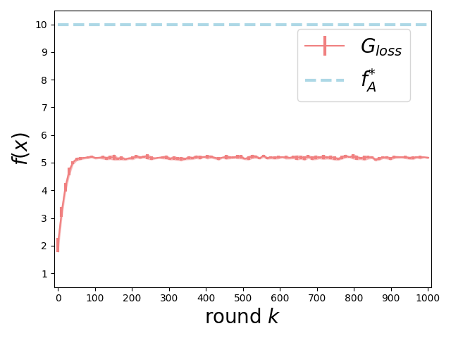
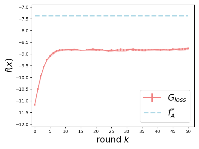
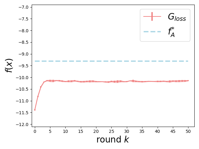
In each iteration of Algorithm 1, we need to compute the gradient guidance GlosssubscriptG𝑙𝑜𝑠𝑠\texttt{G}_{loss}. We set the targeted y𝑦y value at the k𝑘k-th iteration as yk=δ+gkzksubscript𝑦𝑘𝛿superscriptsubscript𝑔𝑘topsubscript𝑧𝑘y_{k}=\delta+g_{k}^{\top}z_{k}, where δksubscript𝛿𝑘\delta_{k} specifies the increment per iteration. The choice on δksubscript𝛿𝑘\delta_{k} is instance-dependent and we set it via tuning for near-optimal in different experiments. For comparing naive gradient with gradient guidance in Figure 5, we set δ=0.2𝛿0.2\delta=0.2 and 0.90.90.9, respectively for using naive gradient G and gradient guidance GlosssubscriptG𝑙𝑜𝑠𝑠\texttt{G}_{loss}. In Figure 6, we choose δ𝛿\delta to be (a) 0.050.050.05, (b) 0.20.20.2, (c) 111, and (d) 111, corresponding to each panel. We initialize Algorithm 1 with a batch of 323232 samples generated by the pre-trained model. Each sample determines an optimization trajectory. We repeat Algorithm 1 for 555 times with different random seeds and report the error bars.

Implementation of Algorithm 2

Algorithm 2 differs from Algorithm 1 in that it allows additional fine-tuning of the pre-trained score network. We adopt a computationally lightweight fine-tuning strategy: We only perform one Adam optimization step using the re-weighted loss given by Eqn. (20) with a batch of 323232 generated samples. We set the learning rate as 106superscript10610^{-6}. This simple strategy already demonstrates good performances as shown in Figure 7. Other implementation details are kept the same as those of Algorithm 1.

We run all experiments using one NVIDIA A100 GPU. Module 1 takes 4.6 seconds to generate a sample. Algorithm 1 takes 76 minutes, and Algorithm 2 takes 91 minutes.

7.2 Results

We first demonstrate our gradient guidance GlosssubscriptG𝑙𝑜𝑠𝑠\texttt{G}_{loss} preserves the subspace structure learned from the pre-trained model. For comparison, we also tested the naive guidance G defined following Lemma 1 (with Σ=IΣ𝐼\Sigma=I). For a quick reference, we repeat the definition here:

G(xt,t):=β(t)(yg𝔼[x0|xt])g,assignGsubscript𝑥𝑡𝑡𝛽𝑡𝑦superscript𝑔top𝔼delimited-[]conditionalsubscript𝑥0subscript𝑥𝑡𝑔\texttt{G}(x_{t},t):=\beta(t)\left(y-g^{\top}\mathbb{E}[x_{0}|x_{t}]\right)g,

where β(t)>0𝛽𝑡0\beta(t)>0 and y𝑦y\in\mathbb{R} are tuning parameters, and 𝔼[x0|xt]𝔼delimited-[]conditionalsubscript𝑥0subscript𝑥𝑡\mathbb{E}[x_{0}|x_{t}] is the conditional expectation of x0subscript𝑥0x_{0} given noise corrupted data xtsubscript𝑥𝑡x_{t}. For implementation, we replace 𝔼[x0|xt]𝔼delimited-[]conditionalsubscript𝑥0subscript𝑥𝑡\mathbb{E}[x_{0}|x_{t}] by its look-ahead estimator 𝔼^[x0|xt]^𝔼delimited-[]conditionalsubscript𝑥0subscript𝑥𝑡\hat{\mathbb{E}}[x_{0}|x_{t}] based on the Tweedie’s formular.

Comparing G and GlosssubscriptG𝑙𝑜𝑠𝑠\texttt{G}_{loss} on Preserving Subspace Structure

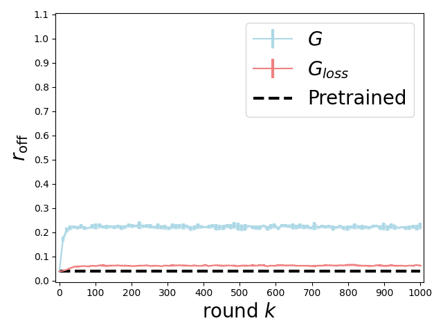
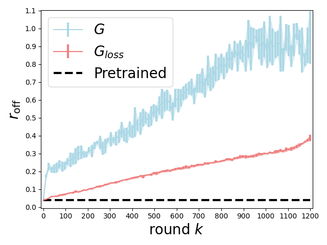
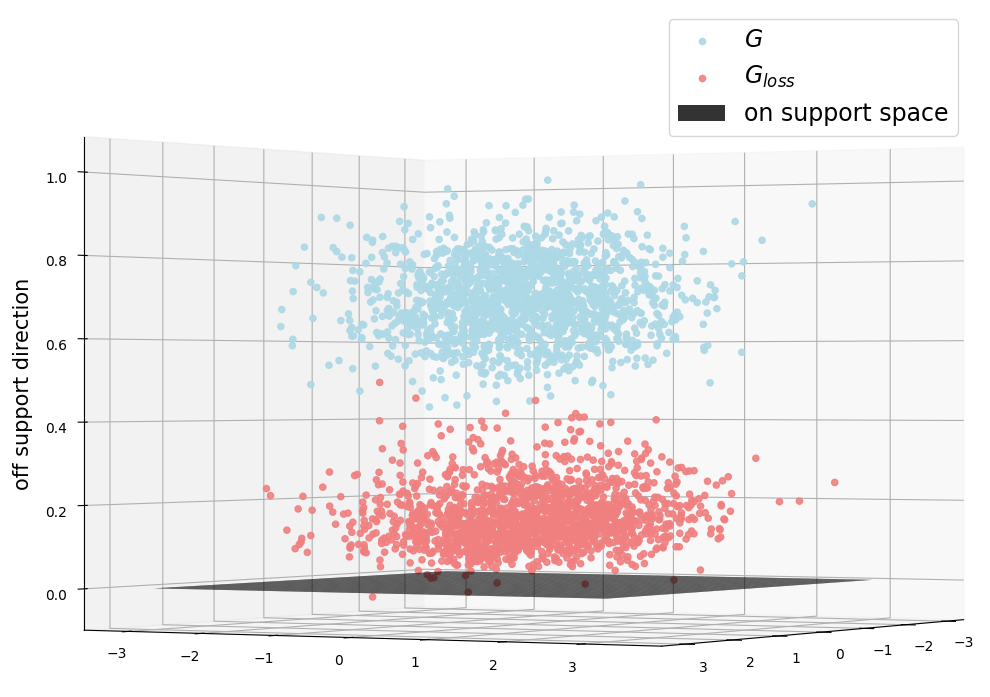
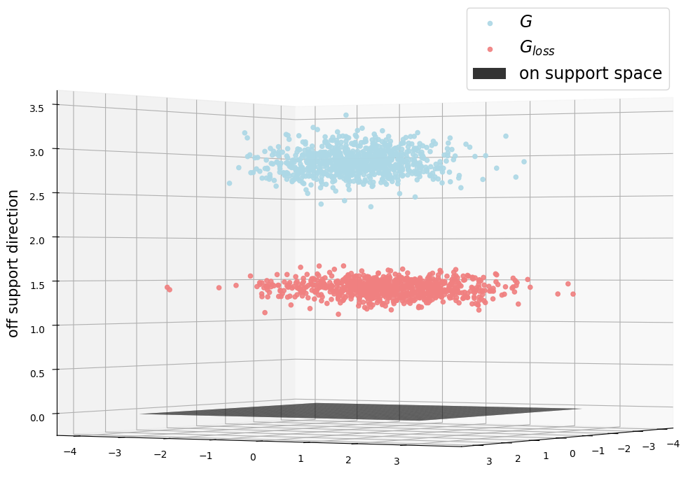
Figure 5(a), (c) verify that the naive gradient G performs much worse than GlosssubscriptG𝑙𝑜𝑠𝑠\texttt{G}_{loss} in preserving the linear subspace structure. It is consistent with our theoretical finding that the gradient guidance GlosssubscriptG𝑙𝑜𝑠𝑠\texttt{G}_{loss} keeps the generated sample close to the latent subspace, with substantially smaller off-support errors. When allowing adaptive score fine-tuning in Algorithm 2, Figure 5(b), (d) show that the off-support error increases as the model gets fine-tuned using self-generated data, due to increasing distribution shift. Even in this case, the naive gradient G leads to much more severe off-support errors as compared to GlosssubscriptG𝑙𝑜𝑠𝑠\texttt{G}_{loss}.

Refer to caption
(a) Algorithm 1
Refer to caption
(b) Algorithm 2
Refer to caption
(c) 300-350 round of (a)
Refer to caption
(d) 1000-1200 round of (b)
Figure 5: Comparison between two types of gradient guidance G and GlosssubscriptG𝑙𝑜𝑠𝑠\texttt{G}_{loss}. We plot the off/on support ratio of the generated samples, denoted by roff=xxsubscript𝑟offnormsubscript𝑥bottomnormsubscript𝑥r_{\mathrm{off}}=\frac{\|{x_{\bot}}\|}{\|{x_{\|}}\|}. The objective function is f1(x)subscript𝑓1𝑥f_{1}(x), with θ𝜃\theta having an off/on-support ratio of 999.

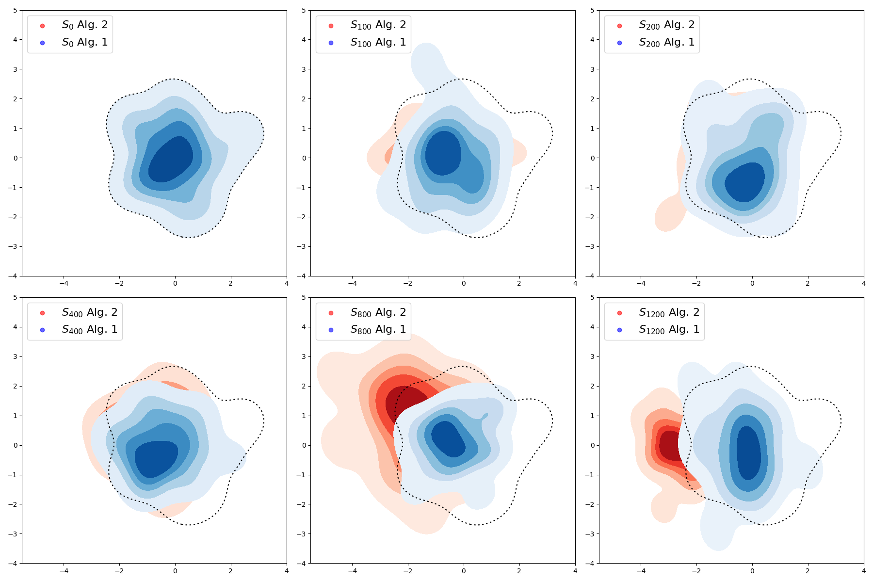
Algorithm 1 Converges to Regularized Optima

We plot the convergence of Algorithm 1 in terms of the objective value in Figure 6. Figure 6 (a),(b) are for the objective function f1=10(θx3)2subscript𝑓110superscriptsuperscript𝜃top𝑥32f_{1}=10-(\theta^{\top}x-3)^{2} as the objective function, while Figure 6(c),(d) are for the objective f2=50.5xbsubscript𝑓250.5delimited-∥∥𝑥𝑏f_{2}=5-0.5\lVert x-b\rVert. We observe that the algorithm converges to reach some sub-optimal objective value, but there remains a gap to the maximal value. This is consistent with our theory that the pre-trained model essentially acts as a regularization in addition to the objective function. Adding gradient guidance alone cannot reach global maxima. This coincides with our theoretical findings in Theorem 3.
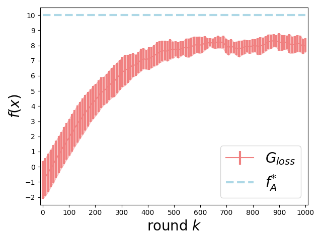
Refer to caption
(a) θ=Aβ𝜃𝐴superscript𝛽\theta=A\beta^{*}
Refer to caption
(b) θθ=9normsubscript𝜃bottomnormsubscript𝜃9\frac{\|{\theta_{\bot}}\|}{\|{\theta_{\|}}\|}=9
Refer to caption
(c) b=41D𝑏4subscript1𝐷b=4\cdot\textbf{1}_{D}
Refer to caption
(d) b𝒩(41D,9ID)similar-to𝑏𝒩4subscript1𝐷9subscript𝐼𝐷b\sim\mathcal{N}(4\cdot\textbf{1}_{D},9\cdot I_{D})
Figure 6: Convergence of Algorithm 1 under different objectives. Objectives are f1(x)subscript𝑓1𝑥f_{1}(x) for (a) and (b), and f2(x)subscript𝑓2𝑥f_{2}(x) for (c) and (d). Parameters θ𝜃\theta and b𝑏b are specified as (a) θ=Aβ𝜃𝐴superscript𝛽\theta=A\beta^{*} with βsuperscript𝛽\beta^{*} being sampled from the unit ball in dsuperscript𝑑\mathbb{R}^{d}; (b) the off/on-support ratio of θ𝜃\theta being 999 (same as Figure 5); (c) and (d) choosing b𝑏b as a homogeneous vector or randomly from a Gaussian distribution. All the experiments adopt the gradient guidance GlosssubscriptG𝑙𝑜𝑠𝑠\texttt{G}_{loss}.

Algorithm 2 Converges to Global Optima

Algorithm 2 converges to the maximal value of the objective function f1=10(θx3)2subscript𝑓110superscriptsuperscript𝜃top𝑥32f_{1}=10-(\theta^{\top}x-3)^{2} as shown in Figure 7(a). In Figure 7(b), we visualize the distribution of generated samples of Algorithm 1 (blue) and 2 (red), respectively, as the iteration evolves. We see that samples from Algorithm 1 mostly stay close to the pre-training data distribution (area described by the dotted contour). In constrast, samples of Algorithm 2 move outside the contour, as the diffusion model gets finetuned using self-generated data.
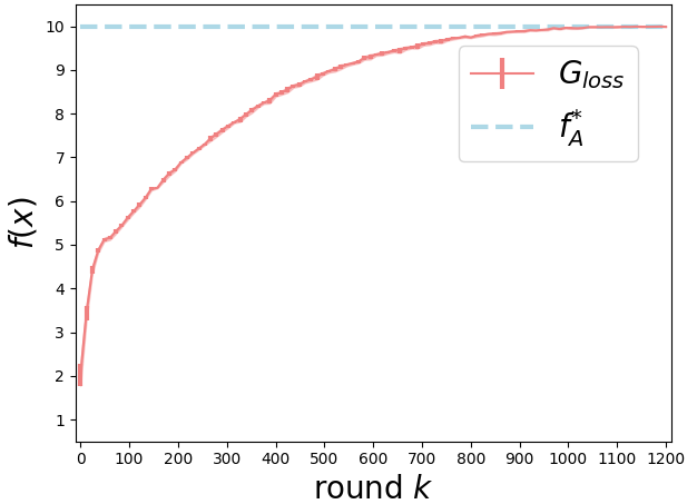
Refer to caption
(a) Convergence of Algorithm 2
Refer to caption
(b) Distribution of generated samples
Figure 7: Convergence of Algorithm 2. Panel (a) plots the objective values achieved by Algorithm 2 as a function of iterations. Here θ𝜃\theta is chosen the same as in Figure 6(b) with off/on-support ratio θθ=9normsubscript𝜃bottomnormsubscript𝜃9\frac{\|{\theta_{\bot}}\|}{\|{\theta_{\|}}\|}=9. Panel (b) visualizes the distribution of the generated samples of Algorithm 2 (red) across the iterations. For comparison, we also visualize the distribution of generated samples of Algorithm 1 (blue).

8 Conclusion

In this paper, we investigate the role and design of gradient guidance for adapting and fine-tuning a pre-trained diffusion model from an optimization perspective. We propose a gradient guidance based on a lookahead loss, as well as two variants of diffusion-based generative optimization algorithm utilizing such guidance. We provide optimization guarantees for adapting/fine-tuning diffusion models towards maximizing any target concave differentiable reward function. Our analysis has also been extended to linear subspace data, where our gradient guidance and adaptive algorithms provably preserve and leverage the latent subspace, thus they achieve faster convergence to near-optimal solutions.

References

  • Ajay et al. (2022) Anurag Ajay, Yilun Du, Abhi Gupta, Joshua Tenenbaum, Tommi Jaakkola, and Pulkit Agrawal. Is conditional generative modeling all you need for decision-making? arXiv preprint arXiv:2211.15657, 2022.
  • Albergo et al. (2023) Michael S Albergo, Nicholas M Boffi, and Eric Vanden-Eijnden. Stochastic interpolants: A unifying framework for flows and diffusions. arXiv preprint arXiv:2303.08797, 2023.
  • Anderson (1982) Brian DO Anderson. Reverse-time diffusion equation models. Stochastic Processes and their Applications, 12(3):313–326, 1982.
  • Bansal et al. (2023) Arpit Bansal, Hong-Min Chu, Avi Schwarzschild, Soumyadip Sengupta, Micah Goldblum, Jonas Geiping, and Tom Goldstein. Universal guidance for diffusion models. In Proceedings of the IEEE/CVF Conference on Computer Vision and Pattern Recognition, pages 843–852, 2023.
  • Benton et al. (2023) Joe Benton, Valentin De Bortoli, Arnaud Doucet, and George Deligiannidis. Linear convergence bounds for diffusion models via stochastic localization. arXiv preprint arXiv:2308.03686, 2023.
  • Black et al. (2023) Kevin Black, Michael Janner, Yilun Du, Ilya Kostrikov, and Sergey Levine. Training diffusion models with reinforcement learning. arXiv preprint arXiv:2305.13301, 2023.
  • Block et al. (2020) Adam Block, Youssef Mroueh, and Alexander Rakhlin. Generative modeling with denoising auto-encoders and langevin sampling. arXiv preprint arXiv:2002.00107, 2020.
  • Bubeck et al. (2015) Sébastien Bubeck et al. Convex optimization: Algorithms and complexity. Foundations and Trends® in Machine Learning, 8(3-4):231–357, 2015.
  • Chen et al. (2023a) Minshuo Chen, Kaixuan Huang, Tuo Zhao, and Mengdi Wang. Score approximation, estimation and distribution recovery of diffusion models on low-dimensional data. arXiv preprint arXiv:2302.07194, 2023a.
  • Chen et al. (2024) Minshuo Chen, Song Mei, Jianqing Fan, and Mengdi Wang. An overview of diffusion models: Applications, guided generation, statistical rates and optimization. arXiv preprint arXiv:2404.07771, 2024.
  • Chen et al. (2022) Sitan Chen, Sinho Chewi, Jerry Li, Yuanzhi Li, Adil Salim, and Anru R Zhang. Sampling is as easy as learning the score: theory for diffusion models with minimal data assumptions. arXiv preprint arXiv:2209.11215, 2022.
  • Chen et al. (2023b) Sitan Chen, Sinho Chewi, Holden Lee, Yuanzhi Li, Jianfeng Lu, and Adil Salim. The probability flow ode is provably fast. arXiv preprint arXiv:2305.11798, 2023b.
  • Chen et al. (2023c) Sitan Chen, Giannis Daras, and Alex Dimakis. Restoration-degradation beyond linear diffusions: A non-asymptotic analysis for ddim-type samplers. In International Conference on Machine Learning, pages 4462–4484. PMLR, 2023c.
  • Chung et al. (2022a) Hyungjin Chung, Jeongsol Kim, Michael T Mccann, Marc L Klasky, and Jong Chul Ye. Diffusion posterior sampling for general noisy inverse problems. arXiv preprint arXiv:2209.14687, 2022a.
  • Chung et al. (2022b) Hyungjin Chung, Byeongsu Sim, Dohoon Ryu, and Jong Chul Ye. Improving diffusion models for inverse problems using manifold constraints. Advances in Neural Information Processing Systems, 35:25683–25696, 2022b.
  • Clark et al. (2023) Kevin Clark, Paul Vicol, Kevin Swersky, and David J Fleet. Directly fine-tuning diffusion models on differentiable rewards. arXiv preprint arXiv:2309.17400, 2023.
  • De Bortoli (2022) Valentin De Bortoli. Convergence of denoising diffusion models under the manifold hypothesis. arXiv preprint arXiv:2208.05314, 2022.
  • De Bortoli et al. (2021) Valentin De Bortoli, James Thornton, Jeremy Heng, and Arnaud Doucet. Diffusion schrödinger bridge with applications to score-based generative modeling. Advances in Neural Information Processing Systems, 34:17695–17709, 2021.
  • Dhariwal and Nichol (2021) Prafulla Dhariwal and Alexander Nichol. Diffusion models beat gans on image synthesis. Advances in neural information processing systems, 34:8780–8794, 2021.
  • Efron (2011) Bradley Efron. Tweedie’s formula and selection bias. Journal of the American Statistical Association, 106(496):1602–1614, 2011.
  • El Alaoui et al. (2023) Ahmed El Alaoui, Andrea Montanari, and Mark Sellke. Sampling from mean-field gibbs measures via diffusion processes. arXiv preprint arXiv:2310.08912, 2023.
  • Fan et al. (2023) Ying Fan, Olivia Watkins, Yuqing Du, Hao Liu, Moonkyung Ryu, Craig Boutilier, Pieter Abbeel, Mohammad Ghavamzadeh, Kangwook Lee, and Kimin Lee. Dpok: Reinforcement learning for fine-tuning text-to-image diffusion models. arXiv preprint arXiv:2305.16381, 2023.
  • Fu et al. (2024) Hengyu Fu, Zhuoran Yang, Mengdi Wang, and Minshuo Chen. Unveil conditional diffusion models with classifier-free guidance: A sharp statistical theory. arXiv preprint arXiv:2403.11968, 2024.
  • Graikos et al. (2022) Alexandros Graikos, Nikolay Malkin, Nebojsa Jojic, and Dimitris Samaras. Diffusion models as plug-and-play priors. Advances in Neural Information Processing Systems, 35:14715–14728, 2022.
  • Gruver et al. (2023) Nate Gruver, Samuel Stanton, Nathan C Frey, Tim GJ Rudner, Isidro Hotzel, Julien Lafrance-Vanasse, Arvind Rajpal, Kyunghyun Cho, and Andrew Gordon Wilson. Protein design with guided discrete diffusion. arXiv preprint arXiv:2305.20009, 2023.
  • Guo et al. (2023) Zhiye Guo, Jian Liu, Yanli Wang, Mengrui Chen, Duolin Wang, Dong Xu, and Jianlin Cheng. Diffusion models in bioinformatics: A new wave of deep learning revolution in action. arXiv preprint arXiv:2302.10907, 2023.
  • Ho and Salimans (2022) Jonathan Ho and Tim Salimans. Classifier-free diffusion guidance. arXiv preprint arXiv:2207.12598, 2022.
  • Ho et al. (2020) Jonathan Ho, Ajay Jain, and Pieter Abbeel. Denoising diffusion probabilistic models. Advances in neural information processing systems, 33:6840–6851, 2020.
  • Kawar et al. (2022) Bahjat Kawar, Michael Elad, Stefano Ermon, and Jiaming Song. Denoising diffusion restoration models. Advances in Neural Information Processing Systems, 35:23593–23606, 2022.
  • Kong et al. (2020) Zhifeng Kong, Wei Ping, Jiaji Huang, Kexin Zhao, and Bryan Catanzaro. Diffwave: A versatile diffusion model for audio synthesis. arXiv preprint arXiv:2009.09761, 2020.
  • Lee et al. (2022a) Holden Lee, Jianfeng Lu, and Yixin Tan. Convergence for score-based generative modeling with polynomial complexity. arXiv preprint arXiv:2206.06227, 2022a.
  • Lee et al. (2022b) Holden Lee, Jianfeng Lu, and Yixin Tan. Convergence of score-based generative modeling for general data distributions. arXiv preprint arXiv:2209.12381, 2022b.
  • Liu et al. (2022) Xingchao Liu, Lemeng Wu, Mao Ye, and Qiang Liu. Let us build bridges: Understanding and extending diffusion generative models. arXiv preprint arXiv:2208.14699, 2022.
  • Liu et al. (2024) Yixin Liu, Kai Zhang, Yuan Li, Zhiling Yan, Chujie Gao, Ruoxi Chen, Zhengqing Yuan, Yue Huang, Hanchi Sun, Jianfeng Gao, et al. Sora: A review on background, technology, limitations, and opportunities of large vision models. arXiv preprint arXiv:2402.17177, 2024.
  • Lugmayr et al. (2022) Andreas Lugmayr, Martin Danelljan, Andres Romero, Fisher Yu, Radu Timofte, and Luc Van Gool. Repaint: Inpainting using denoising diffusion probabilistic models. In Proceedings of the IEEE/CVF Conference on Computer Vision and Pattern Recognition, pages 11461–11471, 2022.
  • Marion et al. (2024) Pierre Marion, Anna Korba, Peter Bartlett, Mathieu Blondel, Valentin De Bortoli, Arnaud Doucet, Felipe Llinares-López, Courtney Paquette, and Quentin Berthet. Implicit diffusion: Efficient optimization through stochastic sampling. arXiv preprint arXiv:2402.05468, 2024.
  • Mei and Wu (2023) Song Mei and Yuchen Wu. Deep networks as denoising algorithms: Sample-efficient learning of diffusion models in high-dimensional graphical models. arXiv preprint arXiv:2309.11420, 2023.
  • Montanari and Wu (2023) Andrea Montanari and Yuchen Wu. Posterior sampling from the spiked models via diffusion processes. arXiv preprint arXiv:2304.11449, 2023.
  • Nichol and Dhariwal (2021) Alexander Quinn Nichol and Prafulla Dhariwal. Improved denoising diffusion probabilistic models. In Proceedings of the International Conference on Machine Learning, pages 8162–8171. PMLR, 2021.
  • Oko et al. (2023) Kazusato Oko, Shunta Akiyama, and Taiji Suzuki. Diffusion models are minimax optimal distribution estimators. arXiv preprint arXiv:2303.01861, 2023.
  • Pope et al. (2021) Phillip Pope, Chen Zhu, Ahmed Abdelkader, Micah Goldblum, and Tom Goldstein. The intrinsic dimension of images and its impact on learning. arXiv preprint arXiv:2104.08894, 2021.
  • Ronneberger et al. (2015) Olaf Ronneberger, Philipp Fischer, and Thomas Brox. U-net: Convolutional networks for biomedical image segmentation. In Medical Image Computing and Computer-Assisted Intervention–MICCAI 2015: 18th International Conference, Munich, Germany, October 5-9, 2015, Proceedings, Part III 18, pages 234–241. Springer, 2015.
  • Roweis and Saul (2000) Sam T Roweis and Lawrence K Saul. Nonlinear dimensionality reduction by locally linear embedding. science, 290(5500):2323–2326, 2000.
  • Song et al. (2020a) Jiaming Song, Chenlin Meng, and Stefano Ermon. Denoising diffusion implicit models. arXiv preprint arXiv:2010.02502, 2020a.
  • Song and Ermon (2019) Yang Song and Stefano Ermon. Generative modeling by estimating gradients of the data distribution. Advances in Neural Information Processing Systems, 32, 2019.
  • Song et al. (2020b) Yang Song, Sahaj Garg, Jiaxin Shi, and Stefano Ermon. Sliced score matching: A scalable approach to density and score estimation. In Uncertainty in Artificial Intelligence, pages 574–584. PMLR, 2020b.
  • Song et al. (2020c) Yang Song, Jascha Sohl-Dickstein, Diederik P Kingma, Abhishek Kumar, Stefano Ermon, and Ben Poole. Score-based generative modeling through stochastic differential equations. arXiv preprint arXiv:2011.13456, 2020c.
  • Tenenbaum et al. (2000) Joshua B Tenenbaum, Vin de Silva, and John C Langford. A global geometric framework for nonlinear dimensionality reduction. science, 290(5500):2319–2323, 2000.
  • Uehara et al. (2024) Masatoshi Uehara, Yulai Zhao, Kevin Black, Ehsan Hajiramezanali, Gabriele Scalia, Nathaniel Lee Diamant, Alex M Tseng, Tommaso Biancalani, and Sergey Levine. Fine-tuning of continuous-time diffusion models as entropy-regularized control. arXiv preprint arXiv:2402.15194, 2024.
  • Wang et al. (2022) Yinhuai Wang, Jiwen Yu, and Jian Zhang. Zero-shot image restoration using denoising diffusion null-space model. arXiv preprint arXiv:2212.00490, 2022.
  • Watson et al. (2023) Joseph L Watson, David Juergens, Nathaniel R Bennett, Brian L Trippe, Jason Yim, Helen E Eisenach, Woody Ahern, Andrew J Borst, Robert J Ragotte, Lukas F Milles, et al. De novo design of protein structure and function with rfdiffusion. Nature, 620(7976):1089–1100, 2023.
  • Wibisono et al. (2024) Andre Wibisono, Yihong Wu, and Kaylee Yingxi Yang. Optimal score estimation via empirical bayes smoothing. arXiv preprint arXiv:2402.07747, 2024.
  • Yang et al. (2023) Ling Yang, Zhilong Zhang, Yang Song, Shenda Hong, Runsheng Xu, Yue Zhao, Wentao Zhang, Bin Cui, and Ming-Hsuan Yang. Diffusion models: A comprehensive survey of methods and applications. ACM Computing Surveys, 56(4):1–39, 2023.
  • Yuan et al. (2023) Hui Yuan, Kaixuan Huang, Chengzhuo Ni, Minshuo Chen, and Mengdi Wang. Reward-directed conditional diffusion: Provable distribution estimation and reward improvement. arXiv preprint arXiv:2307.07055, 2023.

Appendix A Characterization for Output Distribution of Backward Process

In this section, we provide analytical characterizations for the output distribution of the backward process guided by GlosssubscriptG𝑙𝑜𝑠𝑠\texttt{G}_{loss} when the pre-trained score is linear. We first give the result of score matching as follows.

Lemma 2 (Pre-training with Linear Score Functions).

Suppose for pre-training the score network, the class in (20) is

𝒮={s(x,t)=Ctx+bt:CtD×D,btD},𝒮conditional-set𝑠𝑥𝑡subscript𝐶𝑡𝑥subscript𝑏𝑡formulae-sequencesubscript𝐶𝑡superscript𝐷𝐷subscript𝑏𝑡superscript𝐷{\mathcal{S}}=\left\{s(x,t)=C_{t}x+b_{t}:C_{t}\in\mathbb{R}^{D\times D},\,b_{t}\in\mathbb{R}^{D}\right\}, (recall (15))

If we freeze Ctsubscript𝐶𝑡C_{t} in (15), that is, minimizing the score matching objective (20) over the class {s(x,t)=Ctx+bt:btD}conditional-set𝑠𝑥𝑡subscript𝐶𝑡𝑥subscript𝑏𝑡subscript𝑏𝑡superscript𝐷\left\{s(x,t)=C_{t}x+b_{t}:b_{t}\in\mathbb{R}^{D}\right\} gives

sθ(xt,t)=Ct(xtα(t)x¯),subscript𝑠𝜃subscript𝑥𝑡𝑡subscript𝐶𝑡subscript𝑥𝑡𝛼𝑡¯𝑥{s}_{\theta}(x_{t},t)=C_{t}\left(x_{t}-\alpha(t)\bar{x}\right),

where x¯=(i=0kwk,i𝔼x𝒟i[x])/(i=0kwk,i)¯𝑥/superscriptsubscript𝑖0𝑘subscript𝑤𝑘𝑖subscript𝔼𝑥subscript𝒟𝑖delimited-[]𝑥superscriptsubscript𝑖0𝑘subscript𝑤𝑘𝑖\bar{x}=\left(\sum_{i=0}^{k}w_{k,i}{\mathbb{E}}_{x\in\mathcal{D}_{i}}[x]\right)\left/\left(\sum_{i=0}^{k}w_{k,i}\right)\right.. Moreover, minimizing the score matching objective (20) over the class (15) yields

sθ(xt,t)=(α2(t)Σ¯+h(t)ID)1(xtα(t)x¯),subscript𝑠𝜃subscript𝑥𝑡𝑡superscriptsuperscript𝛼2𝑡¯Σ𝑡subscript𝐼𝐷1subscript𝑥𝑡𝛼𝑡¯𝑥{s}_{\theta}(x_{t},t)=-\left(\alpha^{2}(t)\bar{\Sigma}+h(t)I_{D}\right)^{-1}\left(x_{t}-\alpha(t)\bar{x}\right),

where Σ¯=(i=0kwk,i𝔼x𝒟k[(xx¯)(xx¯)])/(i=0kwk,i)¯Σ/superscriptsubscript𝑖0𝑘subscript𝑤𝑘𝑖subscript𝔼𝑥subscript𝒟𝑘delimited-[]𝑥¯𝑥superscript𝑥¯𝑥topsuperscriptsubscript𝑖0𝑘subscript𝑤𝑘𝑖\bar{\Sigma}=\left(\sum_{i=0}^{k}w_{k,i}{\mathbb{E}}_{x\in\mathcal{D}_{k}}\left[(x-\bar{x})(x-\bar{x})^{\top}\right]\right)\left/\left(\sum_{i=0}^{k}w_{k,i}\right)\right. are weighted data covariance.

Proof.

Using the linear score network class 𝒮𝒮{\mathcal{S}} with freezing Ctsubscript𝐶𝑡C_{t}, we cast the score matching loss (20) into

0Ti=0kwk,i𝔼x0𝒟i𝔼xt𝒩(α(t)x0,h(t)ID)[xtlogϕt(xt|x0)s(xt,t)2]dt\displaystyle\quad\int_{0}^{T}\sum_{i=0}^{k}w_{k,i}{\mathbb{E}}_{x_{0}\in\mathcal{D}_{i}}\mathbb{E}_{x_{t}\sim\mathcal{N}\left(\alpha(t)x_{0},h(t)I_{D}\right)}\left[\left\lVert\nabla_{x_{t}}\log\phi_{t}(x_{t}|x_{0})-s(x_{t},t)\right\lVert^{2}\right]\mathop{}\!\mathrm{d}t
=0Ti=0kwk,i𝔼x0𝒟i𝔼xt𝒩(α(t)x0,h(t)ID)[1h(t)(xtα(t)x0)Ctxtbt2]dt\displaystyle=\int_{0}^{T}\sum_{i=0}^{k}w_{k,i}{\mathbb{E}}_{x_{0}\in\mathcal{D}_{i}}\mathbb{E}_{x_{t}\sim\mathcal{N}\left(\alpha(t)x_{0},h(t)I_{D}\right)}\left[\left\lVert-\frac{1}{h(t)}(x_{t}-\alpha(t)x_{0})-C_{t}x_{t}-b_{t}\right\lVert^{2}\right]\mathop{}\!\mathrm{d}t
=0Ti=0kwk,i𝔼x0𝒟i𝔼xt𝒩(α(t)x0,h(t)ID)[(Ct+1h(t)ID)(xtα(t)x0)+(α(t)Ctx0+bt)2]dt\displaystyle=\int_{0}^{T}\sum_{i=0}^{k}w_{k,i}{\mathbb{E}}_{x_{0}\in\mathcal{D}_{i}}\mathbb{E}_{x_{t}\sim\mathcal{N}\left(\alpha(t)x_{0},h(t)I_{D}\right)}\left[\left\lVert\left(C_{t}+\frac{1}{h(t)}I_{D}\right)(x_{t}-\alpha(t)x_{0})+(\alpha(t)C_{t}x_{0}+b_{t})\right\lVert^{2}\right]\mathop{}\!\mathrm{d}t
=(i)0Ti=0kwk,i𝔼x0𝒟i[bt+α(t)Ctx02]+w0Ttrace(h(t)(Ct+1h(t)ID)(Ct+1h(t)ID))dt,\displaystyle\overset{(i)}{=}\int_{0}^{T}\sum_{i=0}^{k}w_{k,i}{\mathbb{E}}_{x_{0}\in\mathcal{D}_{i}}\left[\left\lVert b_{t}+\alpha(t)C_{t}x_{0}\right\lVert^{2}\right]+w\int_{0}^{T}\text{trace}\left(h(t)\left(C_{t}+\frac{1}{h(t)}I_{D}\right)^{\top}\left(C_{t}+\frac{1}{h(t)}I_{D}\right)\right)\mathop{}\!\mathrm{d}t,

where w=i=0kwk,i𝑤superscriptsubscript𝑖0𝑘subscript𝑤𝑘𝑖w=\sum_{i=0}^{k}w_{k,i}, equality (i)𝑖(i) follows from computing the expectation over the conditional Gaussian distribution of xt|x0conditionalsubscript𝑥𝑡subscript𝑥0x_{t}|x_{0}. We note that btsubscript𝑏𝑡b_{t} should minimize i=0kwk,i𝔼x0𝒟i[bt+α(t)Ctx02]\sum_{i=0}^{k}w_{k,i}{\mathbb{E}}_{x_{0}\in\mathcal{D}_{i}}\left[\left\lVert b_{t}+\alpha(t)C_{t}x_{0}\right\lVert^{2}\right] for any t𝑡t, which leads to

b^t=α(t)Ctx¯.subscript^𝑏𝑡𝛼𝑡subscript𝐶𝑡¯𝑥\displaystyle\hat{b}_{t}=-\alpha(t)C_{t}\bar{x}.

Now, we solve Ctsubscript𝐶𝑡C_{t} for the second result. Substituting b^tsubscript^𝑏𝑡\hat{b}_{t} into the optimization objective (20) yields:

0Ti=0kwk,i𝔼x0𝒟i[α(t)Ctx¯α(t)Ctx02]+w0Ttrace(h(t)(Ct+1h(t)ID)(Ct+1h(t)ID))dt\displaystyle\quad\int_{0}^{T}\sum_{i=0}^{k}w_{k,i}{\mathbb{E}}_{x_{0}\in\mathcal{D}_{i}}\left[\left\lVert\alpha(t)C_{t}\bar{x}-\alpha(t)C_{t}x_{0}\right\lVert^{2}\right]+w\int_{0}^{T}\text{trace}\left(h(t)\left(C_{t}+\frac{1}{h(t)}I_{D}\right)^{\top}\left(C_{t}+\frac{1}{h(t)}I_{D}\right)\right)\mathop{}\!\mathrm{d}t
=0Tα2(t)i=0kwk,i𝔼x0𝒟i[Ct(x0x¯)2]+w0Ttrace(h(t)(CtCt+1h(t)Ct+1h(t)Ct+1h2(t)ID))dt.\displaystyle=\int_{0}^{T}\alpha^{2}(t)\sum_{i=0}^{k}w_{k,i}{\mathbb{E}}_{x_{0}\in\mathcal{D}_{i}}\left[\left\lVert C_{t}(x_{0}-\bar{x})\right\lVert^{2}\right]+w\int_{0}^{T}\text{trace}\left(h(t)\left(C_{t}^{\top}C_{t}+\displaystyle\frac{1}{h(t)}C_{t}+\displaystyle\frac{1}{h(t)}C_{t}^{\top}+\displaystyle\frac{1}{h^{2}(t)}I_{D}\right)\right)\mathop{}\!\mathrm{d}t.

Taking the gradient for Ctsubscript𝐶𝑡C_{t}, we get

2α2(t)Cti=0kwk,i𝔼x0𝒟i[(x0x¯)(x0x¯)]+2wh(t)Ct+2wID.2superscript𝛼2𝑡subscript𝐶𝑡superscriptsubscript𝑖0𝑘subscript𝑤𝑘𝑖subscript𝔼subscript𝑥0subscript𝒟𝑖delimited-[]subscript𝑥0¯𝑥superscriptsubscript𝑥0¯𝑥top2𝑤𝑡subscript𝐶𝑡2𝑤subscript𝐼𝐷2\alpha^{2}(t)C_{t}\sum_{i=0}^{k}w_{k,i}{\mathbb{E}}_{x_{0}\in\mathcal{D}_{i}}\left[(x_{0}-\bar{x})(x_{0}-\bar{x})^{\top}\right]+2wh(t)C_{t}+2wI_{D}.

Setting the gradient above to 0, we get the solution for Ctsubscript𝐶𝑡C_{t} as

C^t=(α2(t)w1i=0kwk,i𝔼x0𝒟i[(x0x¯)(x0x¯)]+h(t)ID)1.subscript^𝐶𝑡superscriptsuperscript𝛼2𝑡superscript𝑤1superscriptsubscript𝑖0𝑘subscript𝑤𝑘𝑖subscript𝔼subscript𝑥0subscript𝒟𝑖delimited-[]subscript𝑥0¯𝑥superscriptsubscript𝑥0¯𝑥top𝑡subscript𝐼𝐷1\hat{C}_{t}=-\left(\alpha^{2}(t)w^{-1}\sum_{i=0}^{k}w_{k,i}{\mathbb{E}}_{x_{0}\in\mathcal{D}_{i}}\left[(x_{0}-\bar{x})(x_{0}-\bar{x})^{\top}\right]+h(t)I_{D}\right)^{-1}.

Therefore, the proof is completed.

When wk,0=1,wk,i=0,i[k]formulae-sequencesubscript𝑤𝑘01formulae-sequencesubscript𝑤𝑘𝑖0𝑖delimited-[]𝑘w_{k,0}=1,w_{k,i}=0,i\in[k], Lemma 2 reduces to the pre-traning score matching.

Corollary 1.

Let 𝒟𝒟\mathcal{D} be the pre-training data. Minimizing the score matching objective (3) over the function class (15) gives

sθ(xt,t)=(α2(t)Σ¯+h(t)ID)1(xtα(t)μ¯).subscript𝑠𝜃subscript𝑥𝑡𝑡superscriptsuperscript𝛼2𝑡¯Σ𝑡subscript𝐼𝐷1subscript𝑥𝑡𝛼𝑡¯𝜇{s}_{\theta}(x_{t},t)=-\left(\alpha^{2}(t)\bar{\Sigma}+h(t)I_{D}\right)^{-1}\left(x_{t}-\alpha(t)\bar{\mu}\right). (24)

The following lemma characterizes the output distribution of the backward process guided by GlosssubscriptG𝑙𝑜𝑠𝑠\texttt{G}_{loss} when the pre-trained score is linear.

Lemma 3.

If the pre-trained score sθ(xt,t)subscript𝑠𝜃subscript𝑥𝑡𝑡s_{\theta}(x_{t},t) is (24), substituting the score function with sθ(xt,t)+Gloss(xt,t)subscript𝑠𝜃subscript𝑥𝑡𝑡subscriptG𝑙𝑜𝑠𝑠subscript𝑥𝑡𝑡s_{\theta}(x_{t},t)+\texttt{G}_{loss}(x_{t},t) in the backward SDE (2) yields, when T𝑇T\to\infty,

XT=𝑑𝒩(μ¯+ygμσ2+gΣ¯gΣ¯g,Σ¯Σ¯ggΣ¯σ2+gΣ¯g).superscriptsubscript𝑋𝑇𝑑𝒩¯𝜇𝑦superscript𝑔top𝜇superscript𝜎2superscript𝑔top¯Σ𝑔¯Σ𝑔¯Σ¯Σ𝑔superscript𝑔top¯Σsuperscript𝜎2superscript𝑔top¯Σ𝑔X_{T}^{\leftarrow}\overset{d}{=}\mathcal{N}\left(\bar{\mu}+\frac{y-g^{\top}\mu}{\sigma^{2}+g^{\top}\bar{\Sigma}g}\bar{\Sigma}g,\bar{\Sigma}-\frac{\bar{\Sigma}gg^{\top}\bar{\Sigma}}{\sigma^{2}+g^{\top}\bar{\Sigma}g}\right).

with β(t)𝛽𝑡\beta(t) assigned as β(t)=12(σ2+gΣ¯1(ID+α2(t)Σ¯/h(t))1g)1𝛽𝑡12superscriptsuperscript𝜎2superscript𝑔topsuperscript¯Σ1superscriptsubscript𝐼𝐷superscript𝛼2𝑡¯Σ𝑡1𝑔1\beta(t)=\displaystyle\frac{1}{2}\left(\sigma^{2}+g^{\top}\bar{\Sigma}^{-1}\left(I_{D}+\alpha^{2}(t)\bar{\Sigma}/h(t)\right)^{-1}g\right)^{-1}. Moreover, if pre-training data reside in Span(A)Span𝐴\operatorname{Span}(A) following Assumption 1, it holds XTSpan(A)superscriptsubscript𝑋𝑇Span𝐴X_{T}^{\leftarrow}\in\operatorname{Span}(A).

Proof.

Consider X0=𝑑𝒩(μ¯,Σ¯),Y=gX0+ϵsubscript𝑋0𝑑𝒩¯𝜇¯Σ𝑌superscript𝑔topsubscript𝑋0italic-ϵX_{0}\overset{d}{=}\mathcal{N}\left(\bar{\mu},\bar{\Sigma}\right),Y=g^{\top}X_{0}+\epsilon where ϵ𝒩(0,σ2)similar-toitalic-ϵ𝒩0superscript𝜎2\epsilon\sim\mathcal{N}\left(0,\sigma^{2}\right). Let X0subscript𝑋0X_{0} be the initialization of the forward process. Similar to the proof in Section B.1, we get

[XtY]=𝑑𝒩([α(t)μ¯gμ¯],[α2(t)Σ¯+h(t)IDα(t)Σ¯gα(t)gΣ¯σ2+gΣ¯g]).matrixsubscript𝑋𝑡𝑌𝑑𝒩matrix𝛼𝑡¯𝜇superscript𝑔top¯𝜇matrixsuperscript𝛼2𝑡¯Σ𝑡subscript𝐼𝐷𝛼𝑡¯Σ𝑔𝛼𝑡superscript𝑔top¯Σsuperscript𝜎2superscript𝑔top¯Σ𝑔\displaystyle\begin{bmatrix}X_{t}\\ Y\end{bmatrix}\overset{d}{=}\mathcal{N}\left(\begin{bmatrix}\alpha(t)\bar{\mu}\\ g^{\top}\bar{\mu}\end{bmatrix},\begin{bmatrix}\alpha^{2}(t)\bar{\Sigma}+h(t)I_{D}&\alpha(t)\bar{\Sigma}g\\ \alpha(t)g^{\top}\bar{\Sigma}&\sigma^{2}+g^{\top}\bar{\Sigma}g\end{bmatrix}\right).

Thus, we get sθ(xt,t)subscript𝑠𝜃subscript𝑥𝑡𝑡s_{\theta}(x_{t},t) is exactly the score of marginal distribution of Xtsubscript𝑋𝑡X_{t}, i.e., logpt(xt)=sθ(xt,t)subscript𝑝𝑡subscript𝑥𝑡subscript𝑠𝜃subscript𝑥𝑡𝑡\nabla\log p_{t}(x_{t})=s_{\theta}(x_{t},t). According to the proof in Section B.1, we get sθ(xt,t)+Gloss(xt,t)=logpt(xty)subscript𝑠𝜃subscript𝑥𝑡𝑡subscriptG𝑙𝑜𝑠𝑠subscript𝑥𝑡𝑡subscript𝑝𝑡conditionalsubscript𝑥𝑡𝑦s_{\theta}(x_{t},t)+\texttt{G}_{loss}(x_{t},t)=\nabla\log p_{t}(x_{t}\mid y). Thus, the backward SDE turns out to be

dXt=[12Xt+logpTt(Xty)]dt+dW¯t,X0=𝑑𝒩(0,ID).dsubscriptsuperscript𝑋𝑡delimited-[]12subscriptsuperscript𝑋𝑡subscript𝑝𝑇𝑡conditionalsubscriptsuperscript𝑋𝑡𝑦d𝑡dsubscript¯𝑊𝑡subscriptsuperscript𝑋0𝑑𝒩0subscript𝐼𝐷\mathop{}\!\mathrm{d}X^{\leftarrow}_{t}=\left[\frac{1}{2}X^{\leftarrow}_{t}+\nabla\log p_{T-t}(X^{\leftarrow}_{t}\mid y)\right]\mathop{}\!\mathrm{d}t+\mathop{}\!\mathrm{d}\overline{W}_{t},\quad X^{\leftarrow}_{0}\overset{d}{=}\mathcal{N}\left(0,I_{D}\right). (25)

Since the initial distribution p0(x0y)subscript𝑝0conditionalsubscript𝑥0𝑦p_{0}(x_{0}\mid y) of the forward process can also be obtained by (25) where we replace the initial distribution as pT(xTy)subscript𝑝𝑇conditionalsubscript𝑥𝑇𝑦p_{T}(x_{T}\mid y). According to Girsanov theorem, we get the KL divergence between the terminal distribution pTsuperscriptsubscript𝑝𝑇p_{T}^{\leftarrow} of (25) and p0(x0y)subscript𝑝0conditionalsubscript𝑥0𝑦p_{0}(x_{0}\mid y).

KL(p0pT)=𝔼p0[log(pTφ)],KLconditionalsubscript𝑝0superscriptsubscript𝑝𝑇subscript𝔼subscript𝑝0delimited-[]subscript𝑝𝑇𝜑\text{KL}\left(p_{0}\mid p_{T}^{\leftarrow}\right)=-\mathbb{E}_{p_{0}}\left[\log\left(\frac{p_{T}}{\varphi}\right)\right],

where p0,pTsubscript𝑝0subscript𝑝𝑇p_{0},p_{T} are short hands for p0(x0y)subscript𝑝0conditionalsubscript𝑥0𝑦p_{0}(x_{0}\mid y) and pT(xTy)subscript𝑝𝑇conditionalsubscript𝑥𝑇𝑦p_{T}(x_{T}\mid y), and φ()𝜑\varphi(\cdot) is the density for the standard normal distribution 𝒩(0,ID)𝒩0subscript𝐼𝐷\mathcal{N}\left(0,I_{D}\right). Since in the forward process, pTφsubscript𝑝𝑇𝜑p_{T}\to\varphi when T𝑇T\to\infty, we have KL(p0pT)0KLconditionalsubscript𝑝0superscriptsubscript𝑝𝑇0\text{KL}\left(p_{0}\mid p_{T}^{\leftarrow}\right)\to 0 when T𝑇T\to\infty. We complete the first part of the lemma. As for the second part, if data reside in Span(A)Span𝐴\operatorname{Span}(A) following Assumption 1, we have μ¯=Au¯¯𝜇𝐴¯𝑢\bar{\mu}=A\bar{u} and Σ¯=AΣ¯uA¯Σ𝐴subscript¯Σ𝑢superscript𝐴top\bar{\Sigma}=A\bar{\Sigma}_{u}A^{\top}, where u¯=𝔼x𝒟,u=Ax[u]¯𝑢subscript𝔼formulae-sequence𝑥𝒟𝑢superscript𝐴top𝑥delimited-[]𝑢\bar{u}={\mathbb{E}}_{x\in\mathcal{D},u=A^{\top}x}[u], Σ¯u=𝔼x𝒟,u=Ax[(uu¯)(uu¯)]subscript¯Σ𝑢subscript𝔼formulae-sequence𝑥𝒟𝑢superscript𝐴top𝑥delimited-[]𝑢¯𝑢superscript𝑢¯𝑢top\bar{\Sigma}_{u}={\mathbb{E}}_{x\in\mathcal{D},u=A^{\top}x}[\left(u-\bar{u}\right)\left(u-\bar{u}\right)^{\top}]. Thus, the covariance matrix of XTsubscriptsuperscript𝑋𝑇X^{\leftarrow}_{T} is

Σ¯Σ¯ggΣ¯σ2+gΣ¯g=A[Σ¯uΣ¯uAggAΣ¯uσ2+gΣ¯g]A,¯Σ¯Σ𝑔superscript𝑔top¯Σsuperscript𝜎2superscript𝑔top¯Σ𝑔𝐴delimited-[]subscript¯Σ𝑢subscript¯Σ𝑢superscript𝐴top𝑔superscript𝑔top𝐴subscript¯Σ𝑢superscript𝜎2superscript𝑔top¯Σ𝑔superscript𝐴top\bar{\Sigma}-\frac{\bar{\Sigma}gg^{\top}\bar{\Sigma}}{\sigma^{2}+g^{\top}\bar{\Sigma}g}=A\left[\bar{\Sigma}_{u}-\frac{\bar{\Sigma}_{u}A^{\top}gg^{\top}A\bar{\Sigma}_{u}}{\sigma^{2}+g^{\top}\bar{\Sigma}g}\right]A^{\top},

and due to XTsubscriptsuperscript𝑋𝑇X^{\leftarrow}_{T} follows Gaussian distribution, we get XTSpan(A)superscriptsubscript𝑋𝑇Span𝐴X_{T}^{\leftarrow}\in\operatorname{Span}(A). Thus, the proof is completed. ∎

Appendix B Omitted Proofs in Section 4

\startcontents\printcontents

2Contents   Throughout the proof, we omit the subscript xtsubscript𝑥𝑡x_{t} of \nabla in score function logpt(xt)subscript𝑝𝑡subscript𝑥𝑡\nabla\log p_{t}(x_{t}) and conditional score function logpt(xt|y)subscript𝑝𝑡conditionalsubscript𝑥𝑡𝑦\nabla\log p_{t}(x_{t}|y).

B.1 Proof of Lemma 1

Proof.

Recall {Xt}t0subscriptsubscript𝑋𝑡𝑡0\left\{X_{t}\right\}_{t\geq 0} is the stochastic process from the forward process. X0=𝑑𝒩(μ,Σ),Y=gX0+ϵsubscript𝑋0𝑑𝒩𝜇Σ𝑌superscript𝑔topsubscript𝑋0italic-ϵX_{0}\overset{d}{=}\mathcal{N}\left(\mu,\Sigma\right),Y=g^{\top}X_{0}+\epsilon where ϵ𝒩(0,σ2)similar-toitalic-ϵ𝒩0superscript𝜎2\epsilon\sim\mathcal{N}(0,\sigma^{2}) is independent with X0subscript𝑋0X_{0}. Since X0,Xtsubscript𝑋0subscript𝑋𝑡X_{0},X_{t} and Y𝑌Y are joint Gaussian, we have YXtconditional𝑌subscript𝑋𝑡Y\mid X_{t} also follows Gaussian distribution, denoted as 𝒩(my(xt),σy2(xt))𝒩subscript𝑚𝑦subscript𝑥𝑡superscriptsubscript𝜎𝑦2subscript𝑥𝑡\mathcal{N}\left(m_{y}(x_{t}),\sigma_{y}^{2}(x_{t})\right).Then, the closed form of xtlogpt(yxt)subscriptsubscript𝑥𝑡subscript𝑝𝑡conditional𝑦subscript𝑥𝑡\nabla_{x_{t}}\log p_{t}(y\mid x_{t}) can be derived as

xtlogpt(yxt)=xt[12(ymy(xt)σy(xt))2]xtlogσy(xt).subscriptsubscript𝑥𝑡subscript𝑝𝑡conditional𝑦subscript𝑥𝑡subscriptsubscript𝑥𝑡12superscript𝑦subscript𝑚𝑦subscript𝑥𝑡subscript𝜎𝑦subscript𝑥𝑡2subscriptsubscript𝑥𝑡subscript𝜎𝑦subscript𝑥𝑡\nabla_{x_{t}}\log p_{t}(y\mid x_{t})=-\nabla_{x_{t}}\left[\displaystyle\frac{1}{2}\left(\frac{y-m_{y}(x_{t})}{\sigma_{y}(x_{t})}\right)^{2}\right]-\nabla_{x_{t}}\log\sigma_{y}(x_{t}).

Due to the linearity of Y𝑌Y with regard to X0subscript𝑋0X_{0}, my(xt)subscript𝑚𝑦subscript𝑥𝑡m_{y}(x_{t}) can be computed as

my(xt)=𝔼[yxt]=𝔼[gx0+ϵxt]=𝔼[gx0xt]=g𝔼[x0xt].subscript𝑚𝑦subscript𝑥𝑡𝔼delimited-[]conditional𝑦subscript𝑥𝑡𝔼delimited-[]superscript𝑔topsubscript𝑥0conditionalitalic-ϵsubscript𝑥𝑡𝔼delimited-[]conditionalsuperscript𝑔topsubscript𝑥0subscript𝑥𝑡superscript𝑔top𝔼delimited-[]conditionalsubscript𝑥0subscript𝑥𝑡\displaystyle m_{y}(x_{t})=\mathbb{E}[y\mid x_{t}]=\mathbb{E}[g^{\top}x_{0}+\epsilon\mid x_{t}]=\mathbb{E}[g^{\top}x_{0}\mid x_{t}]=g^{\top}\mathbb{E}[x_{0}\mid x_{t}]. (26)

To get the variance σy2(xt)superscriptsubscript𝜎𝑦2subscript𝑥𝑡\sigma_{y}^{2}(x_{t}), we compute the joint distribution (Xt,Y)subscript𝑋𝑡𝑌(X_{t},Y). In the forward process, given X0=x0subscript𝑋0subscript𝑥0X_{0}=x_{0}, Xtsubscript𝑋𝑡X_{t} can be written as α(t)x0+Zt𝛼𝑡subscript𝑥0subscript𝑍𝑡\alpha(t)x_{0}+Z_{t} for Zt=𝑑𝒩(0,h(t)ID)subscript𝑍𝑡𝑑𝒩0𝑡subscript𝐼𝐷Z_{t}\overset{d}{=}\mathcal{N}(0,h(t)I_{D}) independent of x0subscript𝑥0x_{0}. Due to the linear function assumption, we have

[XtY]=[α(t)ID0IDg10][x0ϵZt].matrixsubscript𝑋𝑡𝑌matrix𝛼𝑡subscript𝐼𝐷0subscript𝐼𝐷superscript𝑔top10matrixsubscript𝑥0italic-ϵsubscript𝑍𝑡\displaystyle\begin{bmatrix}X_{t}\\ Y\end{bmatrix}=\begin{bmatrix}\alpha(t)I_{D}&0&I_{D}\\ g^{\top}&1&0\end{bmatrix}\begin{bmatrix}x_{0}\\ \epsilon\\ Z_{t}\end{bmatrix}.

Observing that the joint distribution of (x0,ϵ,zt)subscript𝑥0italic-ϵsubscript𝑧𝑡(x_{0},\epsilon,z_{t}) is Gaussian, we deduce

[XtY]=𝑑𝒩([α(t)μgμ],[α2(t)Σ+h(t)IDα(t)Σgα(t)gΣσ2+gΣg]).matrixsubscript𝑋𝑡𝑌𝑑𝒩matrix𝛼𝑡𝜇superscript𝑔top𝜇matrixsuperscript𝛼2𝑡Σ𝑡subscript𝐼𝐷𝛼𝑡Σ𝑔𝛼𝑡superscript𝑔topΣsuperscript𝜎2superscript𝑔topΣ𝑔\displaystyle\begin{bmatrix}X_{t}\\ Y\end{bmatrix}\overset{d}{=}\mathcal{N}\left(\begin{bmatrix}\alpha(t)\mu\\ g^{\top}\mu\end{bmatrix},\begin{bmatrix}\alpha^{2}(t)\Sigma+h(t)I_{D}&\alpha(t)\Sigma g\\ \alpha(t)g^{\top}\Sigma&\sigma^{2}+g^{\top}\Sigma g\end{bmatrix}\right).

Thus, we get σy2(xt)=σ2+gΣgα2(t)gΣ(α2(t)Σ+h(t)ID)1Σgsuperscriptsubscript𝜎𝑦2subscript𝑥𝑡superscript𝜎2superscript𝑔topΣ𝑔superscript𝛼2𝑡superscript𝑔topΣsuperscriptsuperscript𝛼2𝑡Σ𝑡subscript𝐼𝐷1Σ𝑔\sigma_{y}^{2}(x_{t})=\sigma^{2}+g^{\top}\Sigma g-\alpha^{2}(t)g^{\top}\Sigma\left(\alpha^{2}(t)\Sigma+h(t)I_{D}\right)^{-1}\Sigma g. Together with the derivation of the mean my(xt)subscript𝑚𝑦subscript𝑥𝑡m_{y}(x_{t}) (26), we get

xtlogpt(yxt)subscriptsubscript𝑥𝑡subscript𝑝𝑡conditional𝑦subscript𝑥𝑡\displaystyle\nabla_{x_{t}}\log p_{t}(y\mid x_{t}) =12σy2(xt)xt[(yg𝔼[x0xt])2]absent12superscriptsubscript𝜎𝑦2subscript𝑥𝑡subscriptsubscript𝑥𝑡superscript𝑦superscript𝑔top𝔼delimited-[]conditionalsubscript𝑥0subscript𝑥𝑡2\displaystyle=-\frac{1}{2\sigma_{y}^{2}(x_{t})}\nabla_{x_{t}}\left[\left(y-g^{\top}\mathbb{E}[x_{0}\mid x_{t}]\right)^{2}\right]
=1σy2(xt)(yg𝔼[x0xt])xt𝔼[x0xt]g.absent1superscriptsubscript𝜎𝑦2subscript𝑥𝑡𝑦superscript𝑔top𝔼delimited-[]conditionalsubscript𝑥0subscript𝑥𝑡subscriptsubscript𝑥𝑡𝔼delimited-[]conditionalsubscript𝑥0subscript𝑥𝑡𝑔\displaystyle=\frac{1}{\sigma_{y}^{2}(x_{t})}\left(y-g^{\top}\mathbb{E}[x_{0}\mid x_{t}]\right)\nabla_{x_{t}}\mathbb{E}[x_{0}\mid x_{t}]g.

To get 𝔼[x0xt]𝔼delimited-[]conditionalsubscript𝑥0subscript𝑥𝑡\mathbb{E}[x_{0}\mid x_{t}], we derive the joint distribution of (X0,Xt)subscript𝑋0subscript𝑋𝑡(X_{0},X_{t}):

[X0Xt]=𝑑𝒩([μα(t)μ],[Σα(t)Σα(t)Σα2(t)Σ+h(t)ID]).matrixsubscript𝑋0subscript𝑋𝑡𝑑𝒩matrix𝜇𝛼𝑡𝜇matrixΣ𝛼𝑡Σ𝛼𝑡Σsuperscript𝛼2𝑡Σ𝑡subscript𝐼𝐷\displaystyle\begin{bmatrix}X_{0}\\ X_{t}\end{bmatrix}\overset{d}{=}\mathcal{N}\left(\begin{bmatrix}\mu\\ \alpha(t)\mu\end{bmatrix},\begin{bmatrix}\Sigma&\alpha(t)\Sigma\\ \alpha(t)\Sigma&\alpha^{2}(t)\Sigma+h(t)I_{D}\end{bmatrix}\right).

Thus, we get 𝔼[x0|xt]=μ+α(t)(α2(t)Σ+h(t)ID)1Σ(xtα(t)μ)𝔼delimited-[]conditionalsubscript𝑥0subscript𝑥𝑡𝜇𝛼𝑡superscriptsuperscript𝛼2𝑡Σ𝑡subscript𝐼𝐷1Σsubscript𝑥𝑡𝛼𝑡𝜇\mathbb{E}[x_{0}|x_{t}]=\mu+\alpha(t)\left(\alpha^{2}(t)\Sigma+h(t)I_{D}\right)^{-1}\Sigma\left(x_{t}-\alpha(t)\mu\right). As a consequence, we have

xtlogpt(yxt)=1σy2(xt)(yg𝔼[x0xt])α(t)(α2(t)Σ+h(t)ID)1Σg.subscriptsubscript𝑥𝑡subscript𝑝𝑡conditional𝑦subscript𝑥𝑡1superscriptsubscript𝜎𝑦2subscript𝑥𝑡𝑦superscript𝑔top𝔼delimited-[]conditionalsubscript𝑥0subscript𝑥𝑡𝛼𝑡superscriptsuperscript𝛼2𝑡Σ𝑡subscript𝐼𝐷1Σ𝑔\nabla_{x_{t}}\log p_{t}(y\mid x_{t})=\displaystyle\frac{1}{\sigma_{y}^{2}(x_{t})}\left(y-g^{\top}\mathbb{E}[x_{0}\mid x_{t}]\right)\alpha(t)\left(\alpha^{2}(t)\Sigma+h(t)I_{D}\right)^{-1}\Sigma g.

Together with the following equality by Woodbury identity, we get the result.

σy2(xt)superscriptsubscript𝜎𝑦2subscript𝑥𝑡\displaystyle\sigma_{y}^{-2}(x_{t}) =(σ2+gΣgα2(t)gΣ(α2(t)Σ+h(t)ID)1Σg)1absentsuperscriptsuperscript𝜎2superscript𝑔topΣ𝑔superscript𝛼2𝑡superscript𝑔topΣsuperscriptsuperscript𝛼2𝑡Σ𝑡subscript𝐼𝐷1Σ𝑔1\displaystyle=\left(\sigma^{2}+g^{\top}\Sigma g-\alpha^{2}(t)g^{\top}\Sigma\left(\alpha^{2}(t)\Sigma+h(t)I_{D}\right)^{-1}\Sigma g\right)^{-1}
=[σ2+gΣ1(ID+α2(t)h(t)Σ)1g]1.absentsuperscriptdelimited-[]superscript𝜎2superscript𝑔topsuperscriptΣ1superscriptsubscript𝐼𝐷superscript𝛼2𝑡𝑡Σ1𝑔1\displaystyle=\left[\sigma^{2}+g^{\top}\Sigma^{-1}\left(I_{D}+\displaystyle\frac{\alpha^{2}(t)}{h(t)}\Sigma\right)^{-1}g\right]^{-1}.

B.2 Proof of Theorem 1

Proof.

We expand the derivative in GlosssubscriptG𝑙𝑜𝑠𝑠\texttt{G}_{loss} as

Gloss(xt,t)=2β(t)(yg𝔼[x0|xt])(xt𝔼[x0|xt])g.subscriptG𝑙𝑜𝑠𝑠subscript𝑥𝑡𝑡2𝛽𝑡𝑦superscript𝑔top𝔼delimited-[]conditionalsubscript𝑥0subscript𝑥𝑡superscriptsubscriptsubscript𝑥𝑡𝔼delimited-[]conditionalsubscript𝑥0subscript𝑥𝑡top𝑔\displaystyle\texttt{G}_{loss}(x_{t},t)=2\beta(t)(y-g^{\top}\mathbb{E}[x_{0}|x_{t}])\left(\nabla_{x_{t}}{\mathbb{E}}[x_{0}|x_{t}]\right)^{\top}g.

It holds 𝔼[x0|xt]=1α(t)(xt+h(t)logpt(xt))𝔼delimited-[]conditionalsubscript𝑥0subscript𝑥𝑡1𝛼𝑡subscript𝑥𝑡𝑡subscript𝑝𝑡subscript𝑥𝑡{\mathbb{E}}[x_{0}|x_{t}]=\frac{1}{\alpha(t)}(x_{t}+h(t)\nabla\log p_{t}(x_{t})). Via the score decomposition under linear subspace data in Chen et al. (2023a, Lemma 1), we have

logpt(xt)=Alogpt𝖫𝖣(Axt)1h(t)(IDAA)xt,subscript𝑝𝑡subscript𝑥𝑡𝐴superscriptsubscript𝑝𝑡𝖫𝖣superscript𝐴topsubscript𝑥𝑡1𝑡subscript𝐼𝐷𝐴superscript𝐴topsubscript𝑥𝑡\displaystyle\nabla\log p_{t}(x_{t})=A\nabla\log p_{t}^{\sf LD}(A^{\top}x_{t})-\frac{1}{h(t)}\left(I_{D}-AA^{\top}\right)x_{t},

where pt𝖫𝖣superscriptsubscript𝑝𝑡𝖫𝖣p_{t}^{\sf LD} denotes the diffused latent distribution, i.e., pt𝖫𝖣(u)=ϕt(u|u0)pu(u0)du0superscriptsubscript𝑝𝑡𝖫𝖣superscript𝑢subscriptitalic-ϕ𝑡conditionalsuperscript𝑢subscript𝑢0subscript𝑝𝑢subscript𝑢0differential-dsubscript𝑢0p_{t}^{\sf LD}(u^{\prime})=\int\phi_{t}(u^{\prime}|u_{0})p_{u}(u_{0})\mathop{}\!\mathrm{d}u_{0}. Recall that ϕtsubscriptitalic-ϕ𝑡\phi_{t} is the Gaussian transition kernel of the forward process and pusubscript𝑝𝑢p_{u} is the density of latent variable u0subscript𝑢0u_{0} in Assumption 1.

To ease the derivation, we denote m(u)=logpt𝖫𝖣(u)+1h(t)u𝑚𝑢superscriptsubscript𝑝𝑡𝖫𝖣𝑢1𝑡𝑢m(u)=\nabla\log p_{t}^{\sf LD}(u)+\frac{1}{h(t)}u. It then holds that

𝔼[x0|xt]𝔼delimited-[]conditionalsubscript𝑥0subscript𝑥𝑡\displaystyle{\mathbb{E}}[x_{0}|x_{t}] =1α(t)(xt+h(t)[Am(Axt)1h(t)xt])absent1𝛼𝑡subscript𝑥𝑡𝑡delimited-[]𝐴𝑚superscript𝐴topsubscript𝑥𝑡1𝑡subscript𝑥𝑡\displaystyle=\frac{1}{\alpha(t)}\left(x_{t}+h(t)\left[Am(A^{\top}x_{t})-\frac{1}{h(t)}x_{t}\right]\right)
=h(t)α(t)Am(Axt).absent𝑡𝛼𝑡𝐴𝑚superscript𝐴topsubscript𝑥𝑡\displaystyle=\frac{h(t)}{\alpha(t)}Am(A^{\top}x_{t}).

As a consequence, we can verify that

xt𝔼[x0|xt]=h(t)α(t)A[m(Axt)]A,subscriptsubscript𝑥𝑡𝔼delimited-[]conditionalsubscript𝑥0subscript𝑥𝑡𝑡𝛼𝑡𝐴delimited-[]𝑚superscript𝐴topsubscript𝑥𝑡superscript𝐴top\displaystyle\nabla_{x_{t}}{\mathbb{E}}[x_{0}|x_{t}]=\frac{h(t)}{\alpha(t)}A\left[\nabla m(A^{\top}x_{t})\right]A^{\top},

where m(Axt)d×d𝑚superscript𝐴topsubscript𝑥𝑡superscript𝑑𝑑\nabla m(A^{\top}x_{t})\in\mathbb{R}^{d\times d} is the Jacobian matrix of m𝑚m at Axtsuperscript𝐴topsubscript𝑥𝑡A^{\top}x_{t}. Plugging the last display into GlosssubscriptG𝑙𝑜𝑠𝑠\texttt{G}_{loss}, we conclude that

Gloss(xt,t)subscriptG𝑙𝑜𝑠𝑠subscript𝑥𝑡𝑡\displaystyle\texttt{G}_{loss}(x_{t},t) =2β(t)(yg𝔼[x0|xt])(xt𝔼[x0|xt])gabsent2𝛽𝑡𝑦superscript𝑔top𝔼delimited-[]conditionalsubscript𝑥0subscript𝑥𝑡superscriptsubscriptsubscript𝑥𝑡𝔼delimited-[]conditionalsubscript𝑥0subscript𝑥𝑡top𝑔\displaystyle=2\beta(t)(y-g^{\top}{\mathbb{E}}[x_{0}|x_{t}])\left(\nabla_{x_{t}}{\mathbb{E}}[x_{0}|x_{t}]\right)^{\top}g
=tgabsentsubscript𝑡𝑔\displaystyle=\ell_{t}\cdot g

for t=2β(t)(yg𝔼[x0|xt])subscript𝑡2𝛽𝑡𝑦superscript𝑔top𝔼delimited-[]conditionalsubscript𝑥0subscript𝑥𝑡\ell_{t}=2\beta(t)(y-g^{\top}{\mathbb{E}}[x_{0}|x_{t}]) and g=(xt𝔼[x0|xt])g=h(t)α(t)A[m(Axt)]AgSpan(A)superscript𝑔superscriptsubscriptsubscript𝑥𝑡𝔼delimited-[]conditionalsubscript𝑥0subscript𝑥𝑡top𝑔𝑡𝛼𝑡𝐴superscriptdelimited-[]𝑚superscript𝐴topsubscript𝑥𝑡topsuperscript𝐴top𝑔Span𝐴g^{\prime}=\left(\nabla_{x_{t}}{\mathbb{E}}[x_{0}|x_{t}]\right)^{\top}g=\frac{h(t)}{\alpha(t)}A\left[\nabla m(A^{\top}x_{t})\right]^{\top}A^{\top}g\in{\rm Span}(A). The proof is complete. ∎

Appendix C Omitted Proofs in Sections 5 and 6

\startcontents\printcontents

2Contents   

C.1 Proof of Theorem 2

Proof.

The proof is a special case of Theorem 3 in Appendix C.2, via setting the representation matrix A=ID𝐴subscript𝐼𝐷A=I_{D}. ∎

C.2 Proof of Theorem 3

Proof of Theorem 3.

Define a filtration {k}k=0K1superscriptsubscriptsubscript𝑘𝑘0𝐾1\left\{\mathcal{H}_{k}\right\}_{k=0}^{K-1} with ksubscript𝑘\mathcal{H}_{k} be the information accumulated after k𝑘k rounds of Alg.1.

0subscript0\displaystyle\mathcal{H}_{0} :=σ(μ¯),assignabsent𝜎¯𝜇\displaystyle:=\sigma(\bar{\mu}),
ksubscript𝑘\displaystyle\mathcal{H}_{k} :=σ(k1,σ(zk1,1,,zk1,Bk1)),k[K].formulae-sequenceassignabsent𝜎subscript𝑘1𝜎subscript𝑧𝑘11subscript𝑧𝑘1subscript𝐵𝑘1𝑘delimited-[]𝐾\displaystyle:=\sigma\left(\mathcal{H}_{k-1},\sigma\left(z_{k-1,1},\ldots,z_{k-1,B_{k-1}}\right)\right),\quad k\in[K].

Define the expectation of samples generated at k𝑘k-th round as

μk:=𝔼[zk,ik1],k[K1].formulae-sequenceassignsubscript𝜇𝑘𝔼delimited-[]conditionalsubscript𝑧𝑘𝑖subscript𝑘1𝑘delimited-[]𝐾1\mu_{k}:=\mathbb{E}[z_{k,i}\mid\mathcal{H}_{k-1}],\quad k\in[K-1].

Applying Corollary 1, we get the pre-trained score as

sθ(xt,t)=(α2(t)Σ¯+h(t)ID)1(xtα(t)μ¯),subscript𝑠𝜃subscript𝑥𝑡𝑡superscriptsuperscript𝛼2𝑡¯Σ𝑡subscript𝐼𝐷1subscript𝑥𝑡𝛼𝑡¯𝜇{s}_{\theta}(x_{t},t)=-\left(\alpha^{2}(t)\bar{\Sigma}+h(t)I_{D}\right)^{-1}\left(x_{t}-\alpha(t)\bar{\mu}\right),

If we set yksubscript𝑦𝑘y_{k} as follows

yk=η(σ2+gkΣ¯gk)+gkμ¯,subscript𝑦𝑘𝜂superscript𝜎2superscriptsubscript𝑔𝑘top¯Σsubscript𝑔𝑘superscriptsubscript𝑔𝑘top¯𝜇y_{k}=\eta\cdot\left(\sigma^{2}+g_{k}^{\top}\bar{\Sigma}g_{k}\right)+g_{k}^{\top}\bar{\mu},

where η=1/λ𝜂1𝜆\eta=1/\lambda. And we choose β(t)𝛽𝑡\beta(t) at k𝑘k-round as β(t)=12(σ2+gk1Σ¯1(ID+α2(t)Σ¯/h(t))1gk1)1𝛽𝑡12superscriptsuperscript𝜎2superscriptsubscript𝑔𝑘1topsuperscript¯Σ1superscriptsubscript𝐼𝐷superscript𝛼2𝑡¯Σ𝑡1subscript𝑔𝑘11\beta(t)=\displaystyle\frac{1}{2}\left(\sigma^{2}+g_{k-1}^{\top}\bar{\Sigma}^{-1}\left(I_{D}+\alpha^{2}(t)\bar{\Sigma}/h(t)\right)^{-1}g_{k-1}\right)^{-1}. Then, Lemma 3 provides the generated distribution in k𝑘k-th round:

𝒩(μ¯+ηΣ¯gk1,Σ¯Σ¯gk1gk1Σ¯σ2+gk1Σ¯gk1).𝒩¯𝜇𝜂¯Σsubscript𝑔𝑘1¯Σ¯Σsubscript𝑔𝑘1superscriptsubscript𝑔𝑘1top¯Σsuperscript𝜎2superscriptsubscript𝑔𝑘1top¯Σsubscript𝑔𝑘1\mathcal{N}\left(\bar{\mu}+\eta\bar{\Sigma}g_{k-1},\bar{\Sigma}-\frac{\bar{\Sigma}g_{k-1}g_{k-1}^{\top}\bar{\Sigma}}{\sigma^{2}+g_{k-1}^{\top}\bar{\Sigma}g_{k-1}}\right). (27)

Define the empirical covariance matrix of the latent variable U𝑈U as Σ¯u=𝔼x𝒟,u=Ax[(uu¯)(uu¯)]subscript¯Σ𝑢subscript𝔼formulae-sequence𝑥𝒟𝑢superscript𝐴top𝑥delimited-[]𝑢¯𝑢superscript𝑢¯𝑢top\bar{\Sigma}_{u}={\mathbb{E}}_{x\in\mathcal{D},u=A^{\top}x}[\left(u-\bar{u}\right)\left(u-\bar{u}\right)^{\top}] where u¯=𝔼𝒟[u]¯𝑢subscript𝔼𝒟delimited-[]𝑢\bar{u}={\mathbb{E}}_{\mathcal{D}}[u]. Then in the subspace setting, the empirical mean and covariance of data X𝑋X can be written as μ¯=AAμ¯¯𝜇𝐴superscript𝐴top¯𝜇\bar{\mu}=AA^{\top}\bar{\mu} and Σ¯=AΣ¯uA¯Σ𝐴subscript¯Σ𝑢superscript𝐴top\bar{\Sigma}=A\bar{\Sigma}_{u}A^{\top} respectively. The mean of the sample zk,isubscript𝑧𝑘𝑖z_{k,i} follows

μk=𝔼[zk,ik1]=AAμ¯+ηAΣ¯uAgk1,subscript𝜇𝑘𝔼delimited-[]conditionalsubscript𝑧𝑘𝑖subscript𝑘1𝐴superscript𝐴top¯𝜇𝜂𝐴subscript¯Σ𝑢superscript𝐴topsubscript𝑔𝑘1\mu_{k}=\mathbb{E}[z_{k,i}\mid\mathcal{H}_{k-1}]=AA^{\top}\bar{\mu}+\eta\cdot A\bar{\Sigma}_{u}A^{\top}g_{k-1},

where gk1=f(z¯k1)subscript𝑔𝑘1𝑓subscript¯𝑧𝑘1g_{k-1}=\nabla f\left(\bar{z}_{k-1}\right) and z¯k1=(1/B)iBzk1,isubscript¯𝑧𝑘11𝐵superscriptsubscript𝑖𝐵subscript𝑧𝑘1𝑖\bar{z}_{k-1}=\left(1/B\right)\sum_{i}^{B}z_{k-1,i}. We rearrange the update rule to show a gradient ascent formula as follows

μksubscript𝜇𝑘\displaystyle\mu_{k} =AAμk1AA(μk1μ¯)+ηAΣ¯uAf(μk1)+ηAΣ¯uA(gk1f(μk1))absent𝐴superscript𝐴topsubscript𝜇𝑘1𝐴superscript𝐴topsubscript𝜇𝑘1¯𝜇𝜂𝐴subscript¯Σ𝑢superscript𝐴top𝑓subscript𝜇𝑘1𝜂𝐴subscript¯Σ𝑢superscript𝐴topsubscript𝑔𝑘1𝑓subscript𝜇𝑘1\displaystyle=AA^{\top}\mu_{k-1}-AA^{\top}\left(\mu_{k-1}-\bar{\mu}\right)+\eta\cdot A\bar{\Sigma}_{u}A^{\top}\nabla f(\mu_{k-1})+\eta\cdot A\bar{\Sigma}_{u}A^{\top}\left(g_{k-1}-\nabla f(\mu_{k-1})\right)
=AAμk1AΣ¯uAAΣ¯u1A(μk1μ¯)+ηAΣ¯uAf(μk1)+ηAΣ¯uA(gk1f(μk1))absent𝐴superscript𝐴topsubscript𝜇𝑘1𝐴subscript¯Σ𝑢superscript𝐴top𝐴superscriptsubscript¯Σ𝑢1superscript𝐴topsubscript𝜇𝑘1¯𝜇𝜂𝐴subscript¯Σ𝑢superscript𝐴top𝑓subscript𝜇𝑘1𝜂𝐴subscript¯Σ𝑢superscript𝐴topsubscript𝑔𝑘1𝑓subscript𝜇𝑘1\displaystyle=AA^{\top}\mu_{k-1}-A\bar{\Sigma}_{u}A^{\top}A\bar{\Sigma}_{u}^{-1}A^{\top}\left(\mu_{k-1}-\bar{\mu}\right)+\eta\cdot A\bar{\Sigma}_{u}A^{\top}\nabla f(\mu_{k-1})+\eta\cdot A\bar{\Sigma}_{u}A^{\top}\left(g_{k-1}-\nabla f(\mu_{k-1})\right)
=AAμk1+ηAΣ¯uA[f(μk1)λAΣ¯u1A(μk1μ¯)]+ηAΣ¯uA(gk1f(μk1)).absent𝐴superscript𝐴topsubscript𝜇𝑘1𝜂𝐴subscript¯Σ𝑢superscript𝐴topdelimited-[]𝑓subscript𝜇𝑘1𝜆𝐴superscriptsubscript¯Σ𝑢1superscript𝐴topsubscript𝜇𝑘1¯𝜇𝜂𝐴subscript¯Σ𝑢superscript𝐴topsubscript𝑔𝑘1𝑓subscript𝜇𝑘1\displaystyle=AA^{\top}\mu_{k-1}+\eta\cdot A\bar{\Sigma}_{u}A^{\top}\left[\nabla f(\mu_{k-1})-\lambda A\bar{\Sigma}_{u}^{-1}A^{\top}\left(\mu_{k-1}-\bar{\mu}\right)\right]+\eta\cdot A\bar{\Sigma}_{u}A^{\top}\left(g_{k-1}-\nabla f(\mu_{k-1})\right).

where λ=1/η𝜆1𝜂\lambda=1/\eta. Define h(x):=f(x)λ/2xμ¯Σ¯12h(x):=f(x)-\lambda/2\left\lVert x-\bar{\mu}\right\lVert^{2}_{\bar{\Sigma}^{-1}}, we have

μksubscript𝜇𝑘\displaystyle\mu_{k} =AAμk1+ηΣ¯h(μk1)+ηΣ¯(gk1f(μk1)).absent𝐴superscript𝐴topsubscript𝜇𝑘1𝜂¯Σsubscript𝜇𝑘1𝜂¯Σsubscript𝑔𝑘1𝑓subscript𝜇𝑘1\displaystyle=AA^{\top}\mu_{k-1}+\eta\cdot\bar{\Sigma}\nabla h(\mu_{k-1})+\eta\cdot\bar{\Sigma}\left(g_{k-1}-\nabla f(\mu_{k-1})\right).

Recall the notation for the optimum: xA,λ=argmaxx=Auh(x)subscriptsuperscript𝑥𝐴𝜆subscriptargmax𝑥𝐴𝑢𝑥x^{\star}_{A,\lambda}=\mathop{\mathrm{argmax}}_{x=Au}h(x). We consider the distance of μksubscript𝜇𝑘\mu_{k} to xA,λsubscriptsuperscript𝑥𝐴𝜆x^{\star}_{A,\lambda} under the semi-norm Σ¯1\left\lVert\cdot\right\lVert_{\bar{\Sigma}^{-1}}.

μkxA,λΣ¯1\displaystyle\left\lVert\mu_{k}-x^{\star}_{A,\lambda}\right\lVert_{\bar{\Sigma}^{-1}} =μk1xA,λ+ηΣ¯h(μk1)+ηΣ¯(gk1f(μk1))Σ¯1\displaystyle=\left\lVert\mu_{k-1}-x^{\star}_{A,\lambda}+\eta\bar{\Sigma}\nabla h(\mu_{k-1})+\eta\bar{\Sigma}\left(g_{k-1}-\nabla f(\mu_{k-1})\right)\right\lVert_{\bar{\Sigma}^{-1}}
μk1xA,λ+ηΣ¯h(μk1)Σ¯1:=I1+ηΣ¯(gk1f(μk1))Σ¯1:=I2.\displaystyle\leq\underbrace{\left\lVert\mu_{k-1}-x^{\star}_{A,\lambda}+\eta\bar{\Sigma}\nabla h(\mu_{k-1})\right\lVert_{\bar{\Sigma}^{-1}}}_{:=I_{1}}+\underbrace{\left\lVert\eta\bar{\Sigma}\left(g_{k-1}-\nabla f(\mu_{k-1})\right)\right\lVert_{\bar{\Sigma}^{-1}}}_{:=I_{2}}. (28)

We bound the second term I2subscript𝐼2I_{2} first. According to f𝑓f is L𝐿L-smooth with respect to Σ¯1\left\lVert\cdot\right\lVert_{\bar{\Sigma}^{-1}}, we have

I2subscript𝐼2\displaystyle I_{2} =ηgk1f(μk1)Σ¯ηLz¯k1μk1Σ¯1,\displaystyle=\eta\left\lVert g_{k-1}-\nabla f(\mu_{k-1})\right\lVert_{\bar{\Sigma}}\leq\eta L\left\lVert\bar{z}_{k-1}-\mu_{k-1}\right\lVert_{\bar{\Sigma}^{-1}},

Lemma 3 shows the distribution of zk1,isubscript𝑧𝑘1𝑖z_{k-1,i}. Therefore, according to concentration inequality for Gaussian distribution, with the probability at least 1δ/K1𝛿𝐾1-\delta/K, it holds

z¯k1μk1Σ¯122log(2Kδ)trace(𝕍(zk1,i)Σ¯1)Bk1.\left\lVert\bar{z}_{k-1}-\mu_{k-1}\right\lVert^{2}_{\bar{\Sigma}^{-1}}\leq 2\log\left(\frac{2K}{\delta}\right)\cdot\displaystyle\frac{\text{trace}\left(\mathbb{V}({z}_{k-1,i})\cdot\bar{\Sigma}^{-1}\right)}{B_{k-1}}.

We have trace(𝕍(zk1,i)Σ¯1)trace(Σ¯Σ¯1)=dtrace𝕍subscript𝑧𝑘1𝑖superscript¯Σ1trace¯Σsuperscript¯Σ1𝑑\text{trace}\left(\mathbb{V}({z}_{k-1,i})\cdot\bar{\Sigma}^{-1}\right)\leq\text{trace}\left(\bar{\Sigma}\cdot\bar{\Sigma}^{-1}\right)=d. Therefore, I2subscript𝐼2I_{2} is bounded by

I2M0/Bk1,subscript𝐼2subscript𝑀0subscript𝐵𝑘1I_{2}\leq M_{0}/\sqrt{B_{k-1}},

where M0:=ηL2log(2Kδ)dassignsubscript𝑀0𝜂𝐿22𝐾𝛿𝑑M_{0}:=\eta L\sqrt{2\log\left(\frac{2K}{\delta}\right)\cdot d}. Next, we consider the first term in (28). Since xA,λsubscriptsuperscript𝑥𝐴𝜆x^{*}_{A,\lambda} is the optimum of hh within Span(A)Span𝐴\operatorname{Span}(A), the gradient h(xA,λ)subscriptsuperscript𝑥𝐴𝜆\nabla h(x^{*}_{A,\lambda}) is in the orthogonal subspace, i.e., Ah(xA,λ)=0superscript𝐴topsubscriptsuperscript𝑥𝐴𝜆0A^{\top}\nabla h(x^{*}_{A,\lambda})=0, thus Σ¯h(xA,λ)=0¯Σsubscriptsuperscript𝑥𝐴𝜆0\bar{\Sigma}\nabla h(x^{*}_{A,\lambda})=0. The first term in (28) can be written as

I12superscriptsubscript𝐼12\displaystyle I_{1}^{2} =(μk1xA,λ)+ηΣ¯(h(μk1)h(xA,λ))Σ¯12\displaystyle=\left\lVert\left(\mu_{k-1}-x^{\star}_{A,\lambda}\right)+\eta\bar{\Sigma}\left(\nabla h(\mu_{k-1})-\nabla h(x^{*}_{A,\lambda})\right)\right\lVert_{\bar{\Sigma}^{-1}}^{2}
=μk1xA,λΣ¯12+η2h(μk1)h(xA,λ)Σ¯2\displaystyle=\left\lVert\mu_{k-1}-x^{\star}_{A,\lambda}\right\lVert_{{\bar{\Sigma}}^{-1}}^{2}+\eta^{2}\left\lVert\nabla h(\mu_{k-1})-\nabla h(x^{*}_{A,\lambda})\right\lVert_{\bar{\Sigma}}^{2}
+2μk1xA,λ,η(h(μk1)h(xA,λ)).2subscript𝜇𝑘1subscriptsuperscript𝑥𝐴𝜆𝜂subscript𝜇𝑘1subscriptsuperscript𝑥𝐴𝜆\displaystyle+2\left<\mu_{k-1}-x^{\star}_{A,\lambda},\eta\left(\nabla h(\mu_{k-1})-\nabla h(x^{*}_{A,\lambda})\right)\right>.

Recall hh is f𝑓f adding a Σ¯1\left\lVert\cdot\right\lVert_{\bar{\Sigma}^{-1}} regularized term. We get hh is (L+λ)𝐿𝜆(L+\lambda)-smooth with respect to semi norm Σ¯1\left\lVert\cdot\right\lVert_{\bar{\Sigma}^{-1}} which is derived from f𝑓f L𝐿L-smooth. Also, hh is λ𝜆\lambda-strongly concave with respect to semi norm Σ¯1\left\lVert\cdot\right\lVert_{\bar{\Sigma}^{-1}} since f𝑓f is concave. According to Lemma 4, we derive

μk1xA,λ,h(μk1)h(xA,λ)λ(L+λ)L+2λμk1xA,λΣ¯121L+2λh(μk1)h(xA,λ)Σ¯2.\displaystyle\left<\mu_{k-1}-x^{\star}_{A,\lambda},\nabla h(\mu_{k-1})-\nabla h(x^{*}_{A,\lambda})\right>\leq-\frac{\lambda(L+\lambda)}{L+2\lambda}\left\lVert\mu_{k-1}-x^{*}_{A,\lambda}\right\lVert^{2}_{\bar{\Sigma}^{-1}}-\frac{1}{L+2\lambda}\left\lVert\nabla h(\mu_{k-1})-\nabla h(x^{*}_{A,\lambda})\right\lVert^{2}_{\bar{\Sigma}}.

Plugin the formula of I1subscript𝐼1I_{1}, we get

I12superscriptsubscript𝐼12\displaystyle I_{1}^{2} (12ηλ(L+λ)L+2λ)μk1xA,λΣ¯12+(η22ηL+2λ)h(μk1)h(xA,λ)Σ¯2.\displaystyle\leq\left(1-\frac{2\eta\lambda(L+\lambda)}{L+2\lambda}\right)\left\lVert\mu_{k-1}-x^{\star}_{A,\lambda}\right\lVert_{{\bar{\Sigma}}^{-1}}^{2}+\left(\eta^{2}-\frac{2\eta}{L+2\lambda}\right)\left\lVert\nabla h(\mu_{k-1})-\nabla h(x^{*}_{A,\lambda})\right\lVert_{\bar{\Sigma}}^{2}.

Since η=1/λ𝜂1𝜆\eta=1/\lambda, it holds η22ηL+2λ>0superscript𝜂22𝜂𝐿2𝜆0\eta^{2}-\displaystyle\frac{2\eta}{L+2\lambda}>0. Due to hh (L+λ)𝐿𝜆(L+\lambda)-smoothness, we get

I12superscriptsubscript𝐼12\displaystyle I_{1}^{2} (12ηλ(L+λ)L+2λ)μk1xA,λΣ¯12+(η22ηL+2λ)(L+λ)2μk1xA,λΣ¯12\displaystyle\leq\left(1-\frac{2\eta\lambda(L+\lambda)}{L+2\lambda}\right)\left\lVert\mu_{k-1}-x^{\star}_{A,\lambda}\right\lVert_{{\bar{\Sigma}}^{-1}}^{2}+\left(\eta^{2}-\frac{2\eta}{L+2\lambda}\right)(L+\lambda)^{2}\left\lVert\mu_{k-1}-x^{\star}_{A,\lambda}\right\lVert_{{\bar{\Sigma}}^{-1}}^{2}
=(1η(L+λ))2μk1xA,λΣ¯12,\displaystyle=\left(1-\eta\left(L+\lambda\right)\right)^{2}\left\lVert\mu_{k-1}-x^{\star}_{A,\lambda}\right\lVert_{{\bar{\Sigma}}^{-1}}^{2},

thus, we get the bound of I1subscript𝐼1I_{1}

I1ζμk1xA,λΣ¯1,I_{1}\leq\zeta\left\lVert\mu_{k-1}-x^{\star}_{A,\lambda}\right\lVert_{{\bar{\Sigma}}^{-1}},

where ζ:=|1η(L+λ)|assign𝜁1𝜂𝐿𝜆\zeta:=\lvert 1-\eta\left(L+\lambda\right)\rvert. Combing the upper bound of I1subscript𝐼1I_{1} and I2subscript𝐼2I_{2}, we get with probability at least 1δ/K1𝛿𝐾1-\delta/K, for 1<kK1𝑘𝐾1<k\leq K,

μkxA,λΣ¯1ζμk1xA,λΣ¯1+M0Bk1.\left\lVert\mu_{k}-x^{\star}_{A,\lambda}\right\lVert_{\bar{\Sigma}^{-1}}\leq\zeta\left\lVert\mu_{k-1}-x^{\star}_{A,\lambda}\right\lVert_{\bar{\Sigma}^{-1}}+\displaystyle\frac{M_{0}}{\sqrt{B_{k-1}}}.

As for k=1𝑘1k=1, by similar derivation, we can obtain μ1xA,λΣ¯1ζz0xA,λΣ¯1\left\lVert\mu_{1}-x^{\star}_{A,\lambda}\right\lVert_{\bar{\Sigma}^{-1}}\leq\zeta\left\lVert{z}_{0}-x^{\star}_{A,\lambda}\right\lVert_{\bar{\Sigma}^{-1}}. By induction, we get with probability at least 1((K1)/K)δ1𝐾1𝐾𝛿1-\left((K-1)/K\right)\delta,

μKxA,λΣ¯1ζKz0xA,λΣ¯1+M0k=1K1ζKk1Bk.\displaystyle\left\lVert\mu_{K}-x^{\star}_{A,\lambda}\right\lVert_{\bar{\Sigma}^{-1}}\leq\zeta^{K}\left\lVert{z}_{0}-x^{\star}_{A,\lambda}\right\lVert_{\bar{\Sigma}^{-1}}+M_{0}\sum_{k=1}^{K-1}\frac{\zeta^{K-k-1}}{\sqrt{B_{k}}}.

Choose Bkζ4k(1ζ)2subscript𝐵𝑘superscript𝜁4𝑘superscript1𝜁2B_{k}\geq\zeta^{-4k}(1-\zeta)^{-2} for all k[K1]𝑘delimited-[]𝐾1k\in[K-1], then we can get

μKxA,λΣ¯1ζK(z0xA,λΣ¯12+M1d)\left\lVert\mu_{K}-x^{\star}_{A,\lambda}\right\lVert_{\bar{\Sigma}^{-1}}\leq\zeta^{K}\left(\left\lVert{z}_{0}-x^{\star}_{A,\lambda}\right\lVert_{\bar{\Sigma}^{-1}}^{2}+{M_{1}\cdot\sqrt{d}}\right) (29)

where M1:=ηL2log(2Kδ)assignsubscript𝑀1𝜂𝐿22𝐾𝛿M_{1}:=\eta L\sqrt{2\log\left(\displaystyle\frac{2K}{\delta}\right)}. Since hh is (L+λ)𝐿𝜆(L+\lambda)-smooth with respect to Σ¯1\left\lVert\cdot\right\lVert_{\bar{\Sigma}^{-1}}, it holds

|h(μK)h(xA,λ)h(xA,λ),μKxA,λ|L+λ2μKxA,λΣ¯12.\lvert h(\mu_{K})-h(x^{*}_{A,\lambda})-\left<\nabla h(x^{*}_{A,\lambda}),\mu_{K}-x^{*}_{A,\lambda}\right>\rvert\leq\displaystyle\frac{L+\lambda}{2}\left\lVert\mu_{K}-x^{*}_{A,\lambda}\right\lVert^{2}_{\bar{\Sigma}^{-1}}.

Considering that h(xA,λ)Span(A)perpendicular-tosubscriptsuperscript𝑥𝐴𝜆Span𝐴\nabla h(x^{*}_{A,\lambda})\perp\operatorname{Span}(A) yields h(xA,λ),μKxA,λ=0subscriptsuperscript𝑥𝐴𝜆subscript𝜇𝐾subscriptsuperscript𝑥𝐴𝜆0\left<\nabla h(x^{*}_{A,\lambda}),\mu_{K}-x^{*}_{A,\lambda}\right>=0, we obtain the following by rearranging the equation above

f(xA,λ)f(μK)𝑓subscriptsuperscript𝑥𝐴𝜆𝑓subscript𝜇𝐾\displaystyle f\left(x^{*}_{A,\lambda}\right)-f(\mu_{K}) λ2(xA,λμ¯Σ¯12μKμ¯Σ¯12)+L+λ2μKxA,λΣ¯12\displaystyle\leq\displaystyle\frac{\lambda}{2}\left(\left\lVert x^{*}_{A,\lambda}-\bar{\mu}\right\lVert^{2}_{\bar{\Sigma}^{-1}}-\left\lVert\mu_{K}-\bar{\mu}\right\lVert^{2}_{\bar{\Sigma}^{-1}}\right)+\displaystyle\frac{L+\lambda}{2}\left\lVert\mu_{K}-x^{*}_{A,\lambda}\right\lVert^{2}_{\bar{\Sigma}^{-1}} (30)
[λμ¯xA,λΣ¯1μKxA,λΣ¯1+(L+λ)μKxA,λΣ¯12].\displaystyle\leq\left[\lambda\left\lVert\bar{\mu}-x^{*}_{A,\lambda}\right\lVert_{\bar{\Sigma}^{-1}}\left\lVert\mu_{K}-x^{*}_{A,\lambda}\right\lVert_{\bar{\Sigma}^{-1}}+(L+\lambda)\left\lVert\mu_{K}-x^{*}_{A,\lambda}\right\lVert^{2}_{\bar{\Sigma}^{-1}}\right].

Substitute (29) into above upper bound, with z0=μ¯subscript𝑧0¯𝜇{z}_{0}=\bar{\mu} we have

f(xA,λ)f(μK)ζK(L+λ)[μ¯xA,λΣ¯12+M12d].\displaystyle f\left(x^{*}_{A,\lambda}\right)-f(\mu_{K})\lesssim\zeta^{K}\cdot(L+\lambda)\left[\left\lVert\bar{\mu}-x^{*}_{A,\lambda}\right\lVert_{\bar{\Sigma}^{-1}}^{2}+M_{1}^{2}d\right].

Since μ¯xA,λΣ¯12=A(μ¯xA,λ)Σ¯u12\left\lVert\bar{\mu}-x^{*}_{A,\lambda}\right\lVert_{\bar{\Sigma}^{-1}}^{2}=\left\lVert A^{\top}\left(\bar{\mu}-x^{*}_{A,\lambda}\right)\right\lVert_{\bar{\Sigma}_{u}^{-1}}^{2} is the distance within Span(A)Span𝐴\operatorname{Span}(A), i.e., 𝒪(d)𝒪𝑑\mathcal{O}(d). Recall η=1/λ𝜂1𝜆\eta=1/\lambda, ζ=|1η(L+λ)|=L/λ𝜁1𝜂𝐿𝜆𝐿𝜆\zeta=\lvert 1-\eta\left(L+\lambda\right)\rvert={L/\lambda}, λ>L𝜆𝐿\lambda>L, and M1=ηL2log(2Kδ)subscript𝑀1𝜂𝐿22𝐾𝛿M_{1}=\eta L\sqrt{2\log\left(\displaystyle\frac{2K}{\delta}\right)}. Therefore, we get the final result:

f(xA,λ)f(μK)λ(Lλ)Kdlog(Kδ),w.p.1δ.less-than-or-similar-to𝑓subscriptsuperscript𝑥𝐴𝜆𝑓subscript𝜇𝐾𝜆superscript𝐿𝜆𝐾𝑑𝐾𝛿w.p.1𝛿f\left(x^{*}_{A,\lambda}\right)-f(\mu_{K})\lesssim\lambda\left(\displaystyle\frac{L}{\lambda}\right)^{K}d\log\left(\frac{K}{\delta}\right),\quad\text{w.p.}1-\delta.

C.3 Proof of Theorem 4

Proof.

Define

0subscript0\displaystyle\mathcal{H}_{0} :=σ(μ¯),assignabsent𝜎¯𝜇\displaystyle:=\sigma(\bar{\mu}),
ksubscript𝑘\displaystyle\mathcal{H}_{k} :=σ(k1,σ(zk1,1,,zk1,Bk1)),k[K1],formulae-sequenceassignabsent𝜎subscript𝑘1𝜎subscript𝑧𝑘11subscript𝑧𝑘1subscript𝐵𝑘1𝑘delimited-[]𝐾1\displaystyle:=\sigma\left(\mathcal{H}_{k-1},\sigma\left(z_{k-1,1},\ldots,z_{k-1,B_{k-1}}\right)\right),\quad k\in[K-1],
μksubscript𝜇𝑘\displaystyle\mu_{k} :=𝔼[zk,ik1],k[K].formulae-sequenceassignabsent𝔼delimited-[]conditionalsubscript𝑧𝑘𝑖subscript𝑘1𝑘delimited-[]𝐾\displaystyle:=\mathbb{E}[z_{k,i}\mid\mathcal{H}_{k-1}],\quad k\in[K].

According to Lemma 2, with freezing Ctsubscript𝐶𝑡C_{t} in class (15), the pre-trained score in Round k𝑘k is sθk+1(xt,t)=(α2(t)Σ¯+h(t)ID)(xtα(t)x¯k)subscript𝑠subscript𝜃𝑘1subscript𝑥𝑡𝑡superscript𝛼2𝑡¯Σ𝑡subscript𝐼𝐷subscript𝑥𝑡𝛼𝑡subscript¯𝑥𝑘s_{\theta_{k+1}}(x_{t},t)=-\left(\alpha^{2}(t)\bar{\Sigma}+h(t)I_{D}\right)\left(x_{t}-\alpha(t)\bar{x}_{k}\right) where x¯k=j=0kwk,jz¯jsubscript¯𝑥𝑘superscriptsubscript𝑗0𝑘subscript𝑤𝑘𝑗subscript¯𝑧𝑗\bar{x}_{k}=\sum_{j=0}^{k}w_{k,j}\bar{z}_{j} and z¯j=𝔼x𝒟j[x]subscript¯𝑧𝑗subscript𝔼𝑥subscript𝒟𝑗delimited-[]𝑥\bar{z}_{j}={\mathbb{E}}_{x\in\mathcal{D}_{j}}[x]. By choosing yksubscript𝑦𝑘y_{k}, and weights wk,jsubscript𝑤𝑘𝑗w_{k,j} as

yksubscript𝑦𝑘\displaystyle y_{k} =ηk(σ2+gkAΣ¯uAgk)+gkAAx¯k,absentsubscript𝜂𝑘superscript𝜎2superscriptsubscript𝑔𝑘top𝐴subscript¯Σ𝑢superscript𝐴topsubscript𝑔𝑘superscriptsubscript𝑔𝑘top𝐴superscript𝐴topsubscript¯𝑥𝑘\displaystyle=\eta_{k}\cdot\left(\sigma^{2}+g_{k}^{\top}A\bar{\Sigma}_{u}A^{\top}g_{k}\right)+g_{k}^{\top}AA^{\top}\bar{x}_{k},
wk,0subscript𝑤𝑘0\displaystyle w_{k,0} =1wkabsent1subscript𝑤𝑘\displaystyle=1-w_{k}
wk,jsubscript𝑤𝑘𝑗\displaystyle w_{k,j} =0,  1j<k,formulae-sequenceabsent01𝑗𝑘\displaystyle=0,\,\,1\leq j<k,
wk,ksubscript𝑤𝑘𝑘\displaystyle w_{k,k} =wk,absentsubscript𝑤𝑘\displaystyle=w_{k},

where ηk>0subscript𝜂𝑘0\eta_{k}>0, 0<wk<10subscript𝑤𝑘10<w_{k}<1 will be specified later. And we choose β(t)𝛽𝑡\beta(t) at Round k𝑘k as β(t)=12(σ2+gk1Σ¯1(ID+α2(t)Σ¯/h(t))1gk1)1𝛽𝑡12superscriptsuperscript𝜎2superscriptsubscript𝑔𝑘1topsuperscript¯Σ1superscriptsubscript𝐼𝐷superscript𝛼2𝑡¯Σ𝑡1subscript𝑔𝑘11\beta(t)=\displaystyle\frac{1}{2}\left(\sigma^{2}+g_{k-1}^{\top}\bar{\Sigma}^{-1}\left(I_{D}+\alpha^{2}(t)\bar{\Sigma}/h(t)\right)^{-1}g_{k-1}\right)^{-1}. Lemma 3 gives the mean of distribution of zk+1,isubscript𝑧𝑘1𝑖z_{k+1,i} as

μk+1=x¯k+ηkΣ¯gk,subscript𝜇𝑘1subscript¯𝑥𝑘subscript𝜂𝑘¯Σsubscript𝑔𝑘\mu_{k+1}=\bar{x}_{k}+\eta_{k}\bar{\Sigma}g_{k}, (31)

and the output distribution

𝒩(x¯K1+ηk1Σ¯gK1,Σ¯Σ¯gK1gK1Σ¯σ2+gK1Σ¯gK1).𝒩subscript¯𝑥𝐾1subscript𝜂𝑘1¯Σsubscript𝑔𝐾1¯Σ¯Σsubscript𝑔𝐾1superscriptsubscript𝑔𝐾1top¯Σsuperscript𝜎2superscriptsubscript𝑔𝐾1top¯Σsubscript𝑔𝐾1\mathcal{N}\left(\bar{x}_{K-1}+\eta_{k-1}\bar{\Sigma}g_{K-1},\bar{\Sigma}-\frac{\bar{\Sigma}g_{K-1}g_{K-1}^{\top}\bar{\Sigma}}{\sigma^{2}+g_{K-1}^{\top}\bar{\Sigma}g_{K-1}}\right). (32)

Applying Lemma 3 yields zk,iSpan(A)subscript𝑧𝑘𝑖SpanA{z}_{k,i}\in\operatorname{Span(A)}, thus, x¯k=AAx¯ksubscript¯𝑥𝑘𝐴superscript𝐴topsubscript¯𝑥𝑘\bar{x}_{k}=AA^{\top}\bar{x}_{k} and Σ¯=AΣ¯uA¯Σ𝐴subscript¯Σ𝑢superscript𝐴top\bar{\Sigma}=A\bar{\Sigma}_{u}A^{\top}, we get the update rule reduced to

μk+1subscript𝜇𝑘1\displaystyle\mu_{k+1} =AA((1wk)μ¯+wkz¯k)+ηk1AΣ¯uAgk1absent𝐴superscript𝐴top1subscript𝑤𝑘¯𝜇subscript𝑤𝑘subscript¯𝑧𝑘subscript𝜂𝑘1𝐴subscript¯Σ𝑢superscript𝐴topsubscript𝑔𝑘1\displaystyle=AA^{\top}\left((1-w_{k})\bar{\mu}+w_{k}\bar{z}_{k}\right)+\eta_{k-1}A\bar{\Sigma}_{u}A^{\top}g_{k-1}
=AAz¯k+ηkAΣ¯uA(f(z¯k)ηk1(1wk)AΣ¯u1A(z¯kμ¯)).absent𝐴superscript𝐴topsubscript¯𝑧𝑘subscript𝜂𝑘𝐴subscript¯Σ𝑢superscript𝐴top𝑓subscript¯𝑧𝑘superscriptsubscript𝜂𝑘11subscript𝑤𝑘𝐴superscriptsubscript¯Σ𝑢1superscript𝐴topsubscript¯𝑧𝑘¯𝜇\displaystyle=AA^{\top}\bar{z}_{k}+\eta_{k}A\bar{\Sigma}_{u}A^{\top}\left(\nabla f(\bar{z}_{k})-\eta_{k}^{-1}(1-w_{k})A\bar{\Sigma}_{u}^{-1}A^{\top}\left(\bar{z}_{k}-\bar{\mu}\right)\right).

We set wk=1ηkλsubscript𝑤𝑘1subscript𝜂𝑘𝜆w_{k}=1-\eta_{k}\lambda and set ηk=ηsubscript𝜂𝑘𝜂\eta_{k}=\eta, where λ,η>0𝜆𝜂0\lambda,\eta>0 will be specified later. Therefore, we have

μk+1=AAz¯k+ηAΣ¯uAhλ(z¯k),subscript𝜇𝑘1𝐴superscript𝐴topsubscript¯𝑧𝑘𝜂𝐴subscript¯Σ𝑢superscript𝐴topsubscript𝜆subscript¯𝑧𝑘\displaystyle\mu_{k+1}=AA^{\top}\bar{z}_{k}+\eta A\bar{\Sigma}_{u}A^{\top}\nabla h_{\lambda}(\bar{z}_{k}), (33)

where hλ(x):=f(x)(λ/2)xμ¯Σ¯12h_{\lambda}(x):=f(x)-(\lambda/2)\left\lVert x-\bar{\mu}\right\lVert^{2}_{\bar{\Sigma}^{-1}}. Define xA,λ=argmaxx=Auhλ(x)subscriptsuperscript𝑥𝐴𝜆subscriptargmax𝑥𝐴𝑢subscript𝜆𝑥x^{\star}_{A,\lambda}=\mathop{\mathrm{argmax}}_{x=Au}h_{\lambda}(x). With some similar steps in proof in Appendix C.2, by choosing Bkζ4k(1ζ)2subscript𝐵𝑘superscript𝜁4𝑘superscript1𝜁2B_{k}\geq\zeta^{-4k}(1-\zeta)^{-2}, together with z0=μ¯subscript𝑧0¯𝜇{z}_{0}=\bar{\mu}, we get

μKxA,λΣ¯1ζK(μ¯xA,λΣ¯1+M1d),w.p.  1δ,\left\lVert\mu_{K}-x^{\star}_{A,\lambda}\right\lVert_{\bar{\Sigma}^{-1}}\lesssim\zeta^{K}\left(\left\lVert\bar{\mu}-x^{\star}_{A,\lambda}\right\lVert_{\bar{\Sigma}^{-1}}+M_{1}\cdot\sqrt{d}\right),\quad\text{w.p.}\,\,1-\delta,

with η=2L+2λ𝜂2𝐿2𝜆\eta=\displaystyle\frac{2}{L+2\lambda}, ζ=|1η(L+λ)|𝜁1𝜂𝐿𝜆\zeta=\lvert 1-\eta(L+\lambda)\rvert and M1=2L(1+η2)log(2Kδ)subscript𝑀12𝐿1superscript𝜂22𝐾𝛿M_{1}=2L\sqrt{(1+\eta^{2})\log\left(\displaystyle\frac{2K}{\delta}\right)}. Also, we can get (30) as in proof in Appendix C.2. We restate it here:

f(xA,λ)f(z~K)λ2(xA,λμ¯Σ¯12μKμ¯Σ¯12)+L+λ2μKxA,λΣ¯12.f\left(x^{*}_{A,\lambda}\right)-f(\tilde{z}_{K})\leq\displaystyle\frac{\lambda}{2}\left(\left\lVert x^{*}_{A,\lambda}-\bar{\mu}\right\lVert^{2}_{\bar{\Sigma}^{-1}}-\left\lVert\mu_{K}-\bar{\mu}\right\lVert^{2}_{\bar{\Sigma}^{-1}}\right)+\displaystyle\frac{L+\lambda}{2}\left\lVert\mu_{K}-x^{*}_{A,\lambda}\right\lVert^{2}_{\bar{\Sigma}^{-1}}. (34)

Since f𝑓f is concave,

f(xA)f(xA,λ)f(xA,λ),xAxA,λ=λΣ¯1(xA,λμ¯),xAxA,λ.𝑓superscriptsubscript𝑥𝐴𝑓subscriptsuperscript𝑥𝐴𝜆𝑓subscriptsuperscript𝑥𝐴𝜆superscriptsubscript𝑥𝐴subscriptsuperscript𝑥𝐴𝜆𝜆superscript¯Σ1subscriptsuperscript𝑥𝐴𝜆¯𝜇superscriptsubscript𝑥𝐴subscriptsuperscript𝑥𝐴𝜆\displaystyle f\left(x_{A}^{\ast}\right)-f\left(x^{*}_{A,\lambda}\right)\leq\left<\nabla f\left(x^{*}_{A,\lambda}\right),x_{A}^{\ast}-x^{*}_{A,\lambda}\right>=\lambda\left<\bar{\Sigma}^{-1}(x^{*}_{A,\lambda}-\bar{\mu}),x_{A}^{\ast}-x^{*}_{A,\lambda}\right>.

Adding (34), it holds

f(xA,λ)f(μK)𝑓subscriptsuperscript𝑥𝐴𝜆𝑓subscript𝜇𝐾\displaystyle f\left(x^{*}_{A,\lambda}\right)-f(\mu_{K}) λ2(xA,λμ¯Σ¯12xA,λxAΣ¯12μKμ¯Σ¯12)+L+λ2μKxA,λΣ¯12.\displaystyle\leq\frac{\lambda}{2}\left(\left\lVert x^{*}_{A,\lambda}-\bar{\mu}\right\lVert^{2}_{\bar{\Sigma}^{-1}}-\left\lVert x^{*}_{A,\lambda}-x_{A}^{\ast}\right\lVert^{2}_{\bar{\Sigma}^{-1}}-\left\lVert\mu_{K}-\bar{\mu}\right\lVert^{2}_{\bar{\Sigma}^{-1}}\right)+\frac{L+\lambda}{2}\left\lVert\mu_{K}-x^{*}_{A,\lambda}\right\lVert^{2}_{\bar{\Sigma}^{-1}}.

Due to (33), we have, it holds w.p. 1δ1𝛿1-\delta,

f(xA,λ)f(μK)[λxAμ¯Σ¯12+(L+λ)ζK(μ¯xA,λΣ¯12+M1d)].f\left(x^{*}_{A,\lambda}\right)-f(\mu_{K})\lesssim\left[\lambda\left\lVert x_{A}^{\ast}-\bar{\mu}\right\lVert^{2}_{\bar{\Sigma}^{-1}}+(L+\lambda)\zeta^{K}\left(\left\lVert\bar{\mu}-x^{*}_{A,\lambda}\right\lVert^{2}_{\bar{\Sigma}^{-1}}+M_{1}d\right)\right].

We choose λ=LlogK/(4K)𝜆𝐿𝐾4𝐾\lambda=L\log K/(4K) and get

f(xA,λ)f(μK)𝑓subscriptsuperscript𝑥𝐴𝜆𝑓subscript𝜇𝐾\displaystyle f\left(x^{*}_{A,\lambda}\right)-f(\mu_{K}) LlogKK[xAμ¯Σ¯12+μ¯xA,λΣ¯12+M1d],w.p.  1δ.\displaystyle\lesssim\frac{L\log K}{K}\cdot\left[\left\lVert x_{A}^{\ast}-\bar{\mu}\right\lVert^{2}_{\bar{\Sigma}^{-1}}+\left\lVert\bar{\mu}-x^{*}_{A,\lambda}\right\lVert^{2}_{\bar{\Sigma}^{-1}}+M_{1}d\right],\,\,\text{w.p.}\,\,1-\delta.

With assuming xA,λ\left\lVert x^{\star}_{A,\lambda}\right\lVert is bounded, we derive

f(xA,λ)f(μK)=𝒪(dL2logKKlog(Kδ)),w.p.  1δ.𝑓subscriptsuperscript𝑥𝐴𝜆𝑓subscript𝜇𝐾𝒪𝑑superscript𝐿2𝐾𝐾𝐾𝛿w.p.1𝛿f\left(x^{*}_{A,\lambda}\right)-f(\mu_{K})=\mathcal{O}\left(\displaystyle\frac{dL^{2}\log K}{K}\cdot\log\left(\frac{K}{\delta}\right)\right),\,\,\text{w.p.}\,\,1-\delta.

C.4 Auxiliary Lemma

The following is a standard result in convex optimization utilized in previous proofs.

Lemma 4.

Let f𝑓f be α𝛼\alpha-strongly concave and β𝛽\beta-smooth with respect to the (semi) norm Σ1\left\lVert\cdot\right\lVert_{\Sigma^{-1}}, for all x𝑥x and y𝑦y, it holds

f(x)f(y),xyαβα+βxyΣ12+1α+βf(x)f(y)Σ2.-\left<\nabla f(x)-\nabla f(y),x-y\right>\geq\displaystyle\frac{\alpha\beta}{\alpha+\beta}\left\lVert x-y\right\lVert^{2}_{\Sigma^{-1}}+\displaystyle\frac{1}{\alpha+\beta}\left\lVert\nabla f(x)-\nabla f(y)\right\lVert^{2}_{\Sigma}. (35)
Proof.

See Bubeck et al. (2015, Lemma 3.11) for a proof. ∎