Abstract

We consider the decay of the inflaton in Starobinsky-like models arising from either an $R+R^{2}$ theory of gravity or $N=1$ no-scale supergravity models. If Standard Model matter is simply introduced to the $R+R^{2}$ theory, the inflaton (which appears when the theory is conformally transformed to the Einstein frame) couples to matter predominantly in Standard Model Higgs kinetic terms. This will typically lead to a reheating temperature of $\sim 3\times 10^{9}$ GeV. However, if the Standard Model Higgs is conformally coupled to curvature, the decay rate may be suppressed and vanishes for a conformal coupling $\xi=1/6$. Nevertheless, inflaton decays through the conformal anomaly leading to a reheating temperature of order $10^{8}$ GeV. The Starobinsky potential may also arise in no-scale supergravity. In this case, the inflaton decays if there is a direct coupling of the inflaton to matter in the superpotential or to gauge fields through the gauge kinetic function. We also discuss the relation between the theories and demonstrate the correspondence between the no-scale models and the conformally coupled $R+R^{2}$ theory (with $\xi=1/6$).

1 1 0 Academic Editor: https://doi.org/ Inflaton decay in No-Scale Supergravity and Starobinsky-like models

UMN–TH–4317/24, FTPI–MINN–24/08

Inflaton decay in No-Scale Supergravity and Starobinsky-like models Yohei Ema¹, Marcos A. G. Garcia², Wenqi Ke¹, Keith A. Olive¹, and Sarunas Verner³ Ema, Y.; Garcia, M. A. G.; Ke, W.; Olive, K.A.; Verner, S. Correspondence: olive@umn.edu

1 Introduction

A key aspect of the difference between the ‘old’ model of inflation, based on a first-order phase transition Guth:1980zm , and the ‘new’ inflationary Universe new is the ability to recover from the era of exponential expansion, or a graceful exit from inflation reviews . In old inflation, bubble percolation was incompatible with resolving the cosmological problems tackled by inflation. In new inflation (and in all subsequent ‘newer’ inflationary models), a graceful exit is a built-in feature. Indeed, a graceful exit is possible regardless of whether inflation takes place at small field values rolling toward large field values (hilltop inflation), or at large field values rolling to the origin in field space (plateau models). The evolution of the field driving inflation, the inflaton, is governed by its equation of motion and begins with a period of slow-roll characterized by exponential expansion, $a\sim e^{H_{I}t}$, where $a$ is the cosmological scale factor and $H_{I}$ is a nearly constant Hubble parameter during inflation. Slow-roll naturally ends with an oscillatory phase where the inflaton oscillates about a minimum, and a matter-dominated phase, $a\sim t^{2/3}$ begins.

However, at some point, inflaton oscillations must give way to a radiation-dominated Universe. This transition is most easily accomplished through the decay of the inflaton dg ; nos , leading to a period of reheating. Provided that the inflaton decay products scatter and thermalize therm , the standard radiation-dominated era of the early Universe is produced. In this review, dedicated to the accomplishments of Professor Dimitri Nanopoulos, we revisit the possibilities for inflaton decay in Starobinsky-like models, and explore these same models when derived from no-scale supergravity no-scale .

The Starobinsky model Staro predates the original models of inflation based on a GUT phase transition, and was an attempt to find a solution for a singularity-free Universe. The model is based on an $R+R^{2}$ theory of gravity, which is conformally equivalent to a theory that combines Einstein gravity with a scalar field, potentially serving as the inflaton WhittStelle . Furthermore, the first calculation of a nearly flat scale-independent density fluctuation spectrum was done in this context MC .

Shortly after the advent of the new inflationary model, it was recognized that supersymmetry may play an important role enot in preventing an inflationary hierarchy problem, which requires the inflaton mass to be $\ll M_{P}$, where $M_{P}=2.4\times 10^{18}$ GeV is the reduced Planck mass. Supergravity is the extension of supersymmetry that incorporates gravitational interactions and it is natural to construct inflationary models consistent with supergravity. However, minimal supergravity models are plagued with the so-called $\eta$ problem eta , in which scalars tend to obtain large (Hubble scale) masses, preventing an extended period of inflation. This problem is alleviated GMO in no-scale supergravity models no-scale , formulated on a maximally symmetric field-space manifold and have been derived as the effective low energy theory from string theory Witten . Of particular interest here is the class of inflationary models based on no-scale supergravity, which yield a model related to the Starobinsky model eno6 ; eno7 ; enov1 .

In this contribution, we will focus on inflaton decay in Starobinsky-like models and related models based on no-scale supergravity. Some of these results may be applicable to $T$-model attractors Kallosh:2013hoa as well. We begin by reviewing the Starobinsky model, augmented with a matter sector that, for simplicity, consists only of the Standard Model Higgs boson (or the supersymmetric Higgs, as the case may be). We also consider the possibility that the Higgs boson is coupled to curvature (with a coupling $\xi$), where the decay rate of the inflaton vanishes when $\xi=1/6$. In this case, the dominant decay mechanism comes from the coupling to $T^{\mu}_{\mu}$ through the conformal anomaly Gorbunov:2012ns . We also consider Starobinsky-like models derived in no-scale supergravity and examine the prospects for decay in these models. In general, inflaton decays in no-scale models are highly suppressed EKOTY ; EGNO4 . In the absence of a direct (superpotential) coupling of the inflaton to the Standard Model, decay to gauge bosons through the gauge kinetic function may be the dominant channel for inflaton decay. For a review on building inflationary models in no-scale supergravity, see Ref. building .

In what follows, we begin with the Starobinsky model as a model of inflation and compare the inflationary observables—the tilt in the perturbation spectrum and the tensor-to-scalar ratio—to CMB results. We consider several possibilities for coupling the Standard Model to the $R+R^{2}$ theory and calculate the inflaton decay rate. Even in the Einstein frame, fields are generally not canonically normalized and we discuss the procedure for determining canonical field coordinates. We also discuss inflaton decay through the conformal anomaly. In Section 3, we discuss the derivation of a Starobinsky-like model in the context of no-scale supergravity. We also review the possibilities for inflaton decay in this context. In this case as well, fields are generally non-canonical, and we briefly review the transformation to canonical field coordinates. Finally, in Section 4, we relate the formulations of the inflationary model in the contexts of $R+R^{2}$ gravity and no-scale supergravity. There is a close correspondence between the two when the Higgs is conformally coupled with $\xi=1/6$. Our conclusions are presented in Section 5.

2 The Starobinsky model and inflaton decays

The Starobinsky model of inflation Staro can be formulated by adding an $R^{2}$ term to the conventional linear Einstein-Hilbert action:

$${\cal A}\;=\;\int d^{4}x\sqrt{-g}\left(-\frac{1}{2}R+\frac{\alpha}{2}R^{2}\right)\,,$$ (1)

where $\alpha$ is a constant. Here, we work in units where $M_{P}=1$. Upon introducing a Lagrange multiplier $-\alpha R^{2}\rightarrow 2\alpha\Phi R+\alpha\Phi^{2}$, this action may be rewritten in the form

$${\cal A}\;=\;-\frac{1}{2}\int d^{4}x\sqrt{-g}\left(R+2\alpha\Phi R+\alpha\Phi^{2}\right)\,.$$ (2)

Then, following the conformal transformation WhittStelle ; Kalara:1990ar

$${\tilde{g}}_{\mu\nu}\;=\;e^{2\Omega}g_{\mu\nu}\;=\;\left(1+2{\alpha}\Phi\right)g_{\mu\nu}\,,$$ (3)

we can rewrite the action in the Einstein frame as

$${\cal A}\;=\;-\frac{1}{2}\int d^{4}x\sqrt{-{\tilde{g}}}\left[{\tilde{R}}-\frac{6{\alpha}^{2}}{(1+2{\alpha}\Phi)^{2}}\left(\partial^{\mu}\Phi\partial_{\mu}\Phi-\frac{\Phi^{2}}{6{\alpha}}\right)\right]\,.$$ (4)

Note the appearance of an additional scalar degree of freedom, with a non-canonical kinetic term and potential $V(\Phi)$. By making a field redefinition, $\phi\equiv\sqrt{3/2}\ln\left(1+2{\alpha}\Phi\right)$, Eq. (4) may be written as:

$${\cal A}\;=\;-\frac{1}{2}\int d^{4}x\sqrt{-{\tilde{g}}}\left[{\tilde{R}}-\partial^{\mu}\phi\partial_{\mu}\phi+\frac{1}{4{\alpha}}\left(1-e^{-\sqrt{\frac{2}{3}}\phi}\right)^{2}\right]\,.$$ (5)

When ${\alpha}=1/6M^{2}$, the potential is now seen with the well-known form of the Starobinsky potential,

$$V(\phi)\;=\;\frac{3}{4}M^{2}\left(1-e^{-\sqrt{\frac{2}{3}}\phi}\right)^{2}\,.$$ (6)

This potential is shown in Fig. 1.

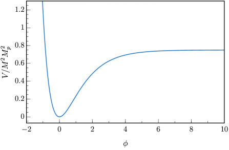
Figure 1: The scalar potential (6) in the Starobinsky model of inflation Staro .

As an inflationary model, the potential (6) leads to observables in excellent agreement with observations by Planck and other CMB experiments Planck ; rlimit ; Tristram:2021tvh . The comparison to experiment is easily made by first computing the slow-roll parameters, $\epsilon$ and $\eta$ for single field inflationary models,

$$\epsilon\;\equiv\;\frac{1}{2}M_{P}^{2}\left(\frac{V^{\prime}}{V}\right)^{2};\;\;\eta\;\equiv\;M_{P}^{2}\left(\frac{V^{\prime\prime}}{V}\right)\,,$$ (7)

where the prime denotes a derivative with respect to the inflaton field $\phi$. Of particular interest is the tilt in the spectrum of scalar perturbations, $n_{s}$ Planck ,

$$n_{s}\; \simeq \;1-6\epsilon_{*}+2\eta_{*}$$ (8)

$$= \;0.965\pm 0.004\;(68\%~{}{\rm CL})\,,$$ (9)

and the tensor-to-scalar ratio, $r$ rlimit ,

$$r\;\simeq\;16\epsilon_{*}<0.036\;(95\%~{}{\rm CL})\,.$$ (10)

The overall inflationary scale, $M$, is set by the amplitude of scalar perturbations, $A_{s}$ Planck ,

$$A_{s}\;=\;\frac{V_{*}}{24\pi^{2}\epsilon_{*}M_{P}^{4}}\simeq 2.1\times 10^{-9}\,.$$ (11)

The number of $e$-folds, $N_{i}$, of inflation between the initial and final values of the inflaton field is given by the formula

$$N_{i}\;\equiv\;\ln\left(\frac{a_{\rm{end}}}{a_{i}}\right)\;=\;\int_{t_{i}}^{t_{\rm{end}}}Hdt\;\simeq\;-\int^{\phi_{\rm{end}}}_{\phi_{i}}\frac{1}{\sqrt{2\epsilon}}\frac{d\phi}{M_{P}}\,.$$ (12)

The number of $e$-folds between when the pivot scale $k_{*}$ exits the horizon and the end of inflation is denoted by $N_{*}$. Inflation ends when $a=a_{\rm end}$ and $\ddot{a}=0$. Typical values of $N_{*}$ are in the range $\sim$ 50-60, depending on the mechanism that ends inflation LiddleLeach ; MRcmb ; Planck .

For the Starobinsky model, it is straightforward to compute the inflationary observable listed above eno6 :

$$A_{s} = \frac{3M^{2}}{8\pi^{2}}\sinh^{4}(\phi/\sqrt{6})\,,$$ (13)

$$\epsilon = \frac{1}{3}\operatorname{csch}^{2}(\phi/\sqrt{6})e^{-\sqrt{2/3}\phi}\,,$$ (14)

$$\eta = \frac{1}{3}\operatorname{csch}^{2}(\phi/\sqrt{6})\left(2e^{-\sqrt{2/3}\phi}-1\right)\,.$$ (15)

For the Starobinsky potential, $\phi_{\rm end}=\phi(a_{\rm end})=0.62M_{P}$ EGNO5 ; egnov and $N_{*}=55$ for $\phi_{*}=5.35M_{P}$. In this case, we find $M=1.25\times 10^{-5}M_{P}\simeq 3\times 10^{13}~{}{\rm GeV}$, $n_{s}=0.965$, and $r=0.0035$.

We show in Fig. 2 taken from Ref. egnov , the 68% and 95% CL regions of the $(n_{s},r)$ plane allowed by the Planck and Keck/BICEP2 data Planck ; rlimit . The (nearly) horizontal line (labeled $\alpha=1$) corresponds to the predictions of the Starobinsky model (6) for $N_{*}\sim 46$ to $\sim 52$ e-folds, corresponding to limits from reheating (see below) 100 GeV $<T_{\text{RH}}<10^{10}$ GeV, the latter corresponding to the upper limit on $T_{\text{RH}}$ from the limit on gravitino production and the relic density of a 100 GeV lightest supersymmetric particle. The other nearly vertical curves correspond to (from left to right), $T_{\text{RH}}=2$ MeV (solid), $N_{*}=50$ (dotted), $T_{\text{RH}}\simeq 5\times 10^{14}$ GeV, obtained when a perturbative decay coupling is $\mathcal{O}(1)$ (with $\Gamma_{\phi}=\frac{y^{2}}{8\pi}m_{\phi}$) (solid), and $N_{*}=60$ (dotted). For the $\alpha$-Starobinsky model eno7 ; KLR ; ENOV3 , we shade the region in green that respects the constraint $T_{\rm reh}>T_{\rm EW}$ and the relic density constraint of $m_{\rm LSP}\simeq 100$ GeV. For more details, see egnov .

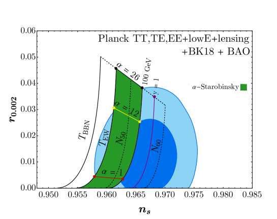
Figure 2: Plot of the CMB observables $n_{s}$ and $r$. The blue shadings correspond to the 68% and 95% confidence level regions from Planck data combined with BICEP2/Keck results Planck ; rlimit . The red dots show the predictions of the $\alpha$-Starobinsky potential with $\alpha=1$ (i.e., the Starobinsky model) for $N_{*}\sim 46$ (left) and $\sim 52$ (right) corresponding to limits from reheating 100 GeV $<T_{\text{RH}}<10^{10}$ GeV. The upper pair of yellow (black) dots are the predictions when $\alpha=12~{}(26)$ (the largest value of $\alpha$ consistent with 68% CL (95% CL) CMB observations and $T_{\text{RH}}\lesssim 10^{10}$ GeV. The vertical lines correspond to the prediction assuming a reheat temperature (or value of $N_{*}$ as appropriate) of $T_{\text{RH}}=2$ MeV, $T_{\text{RH}}=100$ GeV, $N_{*}=50$, $T_{\text{RH}}\simeq 10^{10}$ GeV, $T_{\text{RH}}\simeq 5\times 10^{14}$ GeV, and $N_{*}=60$.

As described above, the $\alpha$-Starobinsky model will inflate and produce density fluctuation in agreement with the experiment. When $\phi<\phi_{\rm end}$, the inflaton begins a period of oscillations, and the energy density in these oscillations scales as $a^{-3}$, typical of a matter-dominated universe. These oscillations continue until inflaton decays occur sufficiently fast to produce radiation. How this occurs depends on how the Standard Model is introduced in the context of inflationary theory and how the inflaton couples to the Standard Model (SM).

We first consider a simple model by adding a complex scalar field $H$ to the $R+R^{2}$ action:

$${\cal A}_{1}\;=\;\int d^{4}x\sqrt{-g}\left(-\frac{1}{2}R+\frac{\alpha}{2}R^{2}+\partial^{\mu}H^{*}\partial_{\mu}H-V(H)\right)\,.$$ (16)

After performing the same conformal transformation (3) and the field redefinition $\phi\equiv\sqrt{3/2}\ln\left(1+2{\alpha}\Phi\right)$, the above action can be rewritten as

$${\cal A}_{1}\;=\;-\frac{1}{2}\int d^{4}x\sqrt{-{\tilde{g}}}\biggl{[} {\tilde{R}}-\partial^{\mu}\phi\partial_{\mu}\phi+\frac{1}{4{\alpha}}\left(1-e^{-\sqrt{\frac{2}{3}}\phi}\right)^{2}$$ (17)

$$-2e^{-\sqrt{\frac{2}{3}}\phi}\partial^{\mu}H^{*}\partial_{\mu}H+2e^{-2\sqrt{\frac{2}{3}}\phi}V(H)\biggr{]}\,.$$

Expanding the second line around the minimum, $\left<\phi\right>=0$, we obtain a canonical kinetic term for the complex scalar, $\partial^{\mu}H^{*}\partial_{\mu}H$, as well as the couplings of the inflaton to $H$:

$${\cal A}_{1}\;\supset\;\int d^{4}x\sqrt{-{\tilde{g}}}\left[-\sqrt{\frac{2}{3}}\phi\partial^{\mu}H^{*}\partial_{\mu}H+2\sqrt{\frac{2}{3}}\phi V(H)\right]\,.$$ (18)

The dominant contribution to the decay $\phi\to HH$ comes from the first term (the 2nd term gives a contribution which is suppressed by the Higgs mass) and the rate is given by

$$\Gamma(\phi\to HH)=\frac{N_{H}}{192\pi}\frac{M^{3}}{M_{P}^{2}}\,,$$ (19)

where $N_{H}=4$ is the number of the real scalar degrees of freedom of the SM Higgs doublet.

It is often useful to perform a field redefinition to obtain canonical fields in a particular background using the Riemann normal coordinates (RNC). The term $\phi\partial^{\mu}H^{*}\partial_{\mu}H$ can be eliminated and the coupling of the inflaton to Higgs is purely a potential interaction. The RNC fields can be obtained quite generally. Consider a Lagrangian of the form

$$\mathcal{L}\;=\;\frac{1}{2}g_{IJ}(\Phi)\partial_{\mu}\Phi^{I}\partial^{\mu}\Phi^{J}-V(\Phi)\,,$$ (20)

where $g_{IJ}(\Phi)$ is a symmetric metric and $V(\Phi)$ is the potential. Here we use the Latin indices $I,J,...,$ for the flavor eigenbasis. To compute the interactions around the minimum, we introduce the field expansion $\Phi^{I}=v^{I}+\phi^{I}$, where $v^{I}$ is the vacuum expectation value and $\phi^{I}$ is the field fluctuation. Following the discussions in Cheung:2021yog ; swamp1 ; swamp2 , the symmetrized covariant derivatives of the potential can be expressed as

$$V_{I_{1}\ldots I_{k}}(v)\;=\;\left.\nabla_{\left(I_{1}\ldots\right.}\nabla_{\left.I_{k}\right)}V(\Phi)\right|_{v}\,,\quad\text{ with }\left.\quad\partial_{I}V(\Phi)\right|_{v}=0\,,$$ (21)

where the covariant derivatives are symmetrized and include all permutations multiplied by a factor of symmetry $1/n!$. Here we take the derivatives with respect to field $\Phi^{I}$, evaluated at their VEV $v^{I}$. The Christoffel symbols are given by

$$\Gamma^{I}_{JK}\;=\;\frac{1}{2}g^{IL}\left(g_{KL,J}+g_{LJ,K}-g_{JK,L}\right)\,.$$ (22)

Using these definitions, we find that the canonically normalized mass matrix at the minimum is given by $V_{IJ}(v)=\partial_{I}\partial_{J}V(\Phi)|_{v}$. To canonically normalize the fields and transform from the flavor to mass eigenbasis, we introduce a tetrad that flattens the metric

$$g_{IJ}(v)e_{i}^{I}(v)e_{j}^{J}(v)\;=\;\delta_{ij}\,.$$ (23)

Here, the lowercase letters correspond to the mass eigenbasis, and the indices may be raised or lower using the Kronecker delta $\delta_{ij}$ or $\delta^{ij}$. The inverse tetrad can be computed using the expression $e^{i}_{I}=\delta^{ij}e_{j}^{~{}J}g_{JI}$.

In Riemann normal coordinates, there are no cubic derivative interactions, which significantly simplifies the computation. Thus, in this case, the cubic interaction can arise only from the potential terms. From the action (17), we find that the field metric of the kinetic terms $\frac{1}{2}g_{IJ}(\Phi)\partial_{\mu}\Phi^{I}\partial^{\mu}\Phi^{J}$ can be expressed as

$$g_{IJ}\;=\;{\rm{diag}}\left(1\,,2e^{-\sqrt{\frac{2}{3}}\phi}\,,2e^{-\sqrt{\frac{2}{3}}\phi}\right)\,,$$ (24)

where $\Phi=(\phi,\,\mathrm{Re}\,H,\,\mathrm{Im}\,H)$. At the minimum, the VEVs of these fields are $v=(0,0,0)$. We find that the tetrad at the minimum is given by

$$e_{i}^{I}(v)={\rm diag}\left(1,\frac{1}{\sqrt{2}},\frac{1}{\sqrt{2}}\right)\,.$$ (25)

Finally, we compute the three-particle scattering amplitude using Eq. (21) that includes a symmetry factor for two identical final states in the amplitude. To compute the scattering amplitude in the mass eigenbasis, we use

$$V_{IJK}(v)e_{i}^{I}(v)e_{j}^{J}(v)e_{k}^{K}(v)\;=\;V_{ijk}(v)\,,$$ (26)

and find

$$V_{\phi,\,\mathrm{Re}\,H,\,\mathrm{Re}\,H}\;=\;V_{\phi,\,\mathrm{Im}\,H,\,\mathrm{Im}\,H}\;=\;-\frac{M^{2}}{\sqrt{6}}\,.$$ (27)

These couplings lead to the decay rate (19). For more details on how to use the RNC to compute the scattering amplitudes, see Refs. Cheung:2021yog ; swamp1 ; swamp2 .

Another alternative description of the model entails a conformal transform into the conformal frame where all the scalar fields conformally couple to the gravity. This is achieved by the conformal transformation

$$g_{c\mu\nu}=e^{2{\Omega}_{c}}g_{\mu\nu}\,,$$ (28)

with the inflaton $\phi$ and the conformal factor satisfying

$$\phi_{c}=\sqrt{6}\left(e^{-{\Omega}_{c}}-1\right)\,,\quad 1+2\alpha\Phi=e^{2{\Omega}_{c}}\left(1-\frac{\phi_{c}^{2}+2|H_{c}|^{2}}{6}\right)\,,\quad H=e^{{\Omega}_{c}}H_{c}\,.$$ (29)

Then the above action can be rewritten as Ema:2020zvg

$$\mathcal{A}_{1}=\int d^{4}x\sqrt{-g_{c}} \left[-\frac{1}{2}R_{c}\left(1-\frac{\phi_{c}^{2}+2|H_{c}|^{2}}{6}\right)+\frac{1}{2}\partial^{\mu}\phi_{c}\partial_{\mu}\phi_{c}+\partial^{\mu}H_{c}^{*}\partial_{\mu}H_{c}\right.$$

$$\left.-\left(1+\frac{\phi_{c}}{\sqrt{6}}\right)^{4}V\left(\frac{H_{c}}{1+\phi_{c}/\sqrt{6}}\right)-\frac{3M^{2}}{4}\left(\sqrt{\frac{2}{3}}\phi_{c}+\frac{\phi_{c}^{2}}{3}+\frac{|H_{c}|^{2}}{3}\right)^{2}\right]\,.$$ (30)

In this frame, the scalar fields are canonical and conformally coupled to gravity without any kinetic mixing, and the decay is induced by the cubic interaction $\phi_{c}|H_{c}|^{2}$ from the potential. Focusing on the Standard Model Higgs with $V(H)=m^{2}|H|^{2}+\lambda|H|^{4}$, the decay is predominantly induced by the last term in Eq. (30), and we recover the decay rate given in Eq. (19), which is expected due to frame independence.

One may also introduce a non-minimal coupling to gravity $\xi RH^{*}H$:

$${\cal A}_{2}\;=\;\int d^{4}x\sqrt{-g}\left(-\frac{1}{2}R+\frac{\alpha}{2}R^{2}+\partial^{\mu}H^{*}\partial_{\mu}H+\xi RH^{*}H-V(H)\right)\,.$$ (31)

The conformal transformation in this case is

$${\tilde{g}}_{\mu\nu}\;=\;e^{2\Omega}g_{\mu\nu}\;=\;\left(1+2{\alpha}\Phi-2\xi|H|^{2}\right)g_{\mu\nu}\,.$$ (32)

In the Einstein frame, this is equivalent to

$${\cal A}_{2}\;=\;-\frac{1}{2}\int d^{4}x\sqrt{-{\tilde{g}}}\biggl{[} {\tilde{R}}-\partial^{\mu}\phi\partial_{\mu}\phi+\frac{1}{4{\alpha}}\left(1-e^{-\sqrt{\frac{2}{3}}\phi}+2\xi e^{-\sqrt{\frac{2}{3}}\phi}H^{*}H\right)^{2}$$ (33)

$$-2e^{-\sqrt{\frac{2}{3}}\phi}\partial^{\mu}H^{*}\partial_{\mu}H+2e^{-2\sqrt{\frac{2}{3}}\phi}V(H)\biggr{]}\,,$$

where now $\phi=\sqrt{3/2}\ln(1+2\alpha\Phi-2\xi|H|^{2})$.

To compute the decay rate in this frame, one can again expand the couplings around the minimum, which gives rise to the following dominant trilinear couplings:

$${\cal A}_{2}\;\supset\;\int d^{4}x\sqrt{-{\tilde{g}}}\left[-\frac{1}{2\alpha}\xi\sqrt{\frac{2}{3}}\phi|H|^{2}-\frac{2}{\sqrt{6}}\phi\partial^{\mu}H^{*}\partial_{\mu}H\right]\,.$$ (34)

The rate is then

$$\Gamma(\phi\to HH)=\frac{N_{H}(1-6\xi)^{2}}{192\pi}\frac{M^{3}}{M_{P}^{2}}\,.$$ (35)

Alternatively, we may move to the conformal frame by

$$g_{c\mu\nu}=e^{2{\Omega}_{c}}g_{\mu\nu}\,,$$ (36)

with the inflaton $\phi$ and the conformal factor satisfying

$$\phi_{c}=\sqrt{6}\left(e^{-{\Omega}_{c}}-1\right)\,,\quad 1+2\alpha\Phi-2\xi|H|^{2}=e^{2{\Omega}_{c}}\left(1-\frac{\phi_{c}^{2}+2|H_{c}|^{2}}{6}\right)\,,\quad H=e^{{\Omega}_{c}}H_{c}\,,$$ (37)

and we obtain Ema:2020zvg

$$\mathcal{A}_{2}=\int d^{4}x\sqrt{-g_{c}} \left[-\frac{1}{2}R_{c}\left(1-\frac{\phi_{c}^{2}+2|H_{c}|^{2}}{6}\right)+\frac{1}{2}\partial^{\mu}\phi_{c}\partial_{\mu}\phi_{c}+\partial^{\mu}H_{c}^{*}\partial_{\mu}H_{c}\right.$$

$$\left.-\left(1+\frac{\phi_{c}}{\sqrt{6}}\right)^{4}V\left(\frac{H_{c}}{1+\phi_{c}/\sqrt{6}}\right)-\frac{3M^{2}}{4}\left(\sqrt{\frac{2}{3}}\phi_{c}+\frac{\phi_{c}^{2}}{3}+\frac{1-6\xi}{3}|H_{c}|^{2}\right)^{2}\right]\,.$$ (38)

This form of action makes it manifest that the interaction between the inflaton and the Higgs is controlled by the combination $1-6\xi$. The decay is again induced by the cubic interaction $\phi_{c}|H_{c}|^{2}$ from the last term in the potential, and not surprisingly the rate is given by Eq. (35). Note that a very large negative value for $\xi$ forces the Higgs to participate in the inflationary dynamics, making it the so-called Higgs-$R^{2}$ inflation model Wang:2017fuy . In this case, the (p)reheating dynamics can be non-perturbative He:2018mgb , and we do not consider this regime in the following.

The above formula shows that, if the Higgs conformally couples to gravity, with $\xi=1/6$, the inflaton does not decay into the Higgs. In this case, the inflaton predominantly decays into Standard Model gauge bosons through the trace anomaly Gorbunov:2012ns . In general, the coupling between the inflaton and Standard Model particles in the Starobinsky model is expressed to the lowest order as

$$\mathcal{L}=\frac{1}{\sqrt{6}}\phi{T^{\mu}}_{\mu}\,,$$ (39)

where ${T^{\mu}}_{\mu}$ is the trace of the stress-energy tensor. One can see that Eqs. (18) and (34) indeed take this form. If the matter sector is (classically) conformal, and assuming the absence of direct coupling between the gauge sector and the gravity beyond the minimal one in the original frame, ${T^{\mu}}_{\mu}$ is predominantly sourced by the trace anomaly. The origin of the trace anomaly depends on the regularization scheme (although the final result itself does not) Kamada:2019pmx . For instance, in dimensional regularization, the inflaton couples to the gauge bosons as $\epsilon\phi F_{\mu\nu}F^{\mu\nu}$, with the spacetime dimension $d=4-2\epsilon$, after the conformal transformation. This factor of $\epsilon$ is compensated by the $1/\epsilon$ pole arising from the wavefunction renormalization (and self-interactions in the non-abelian case), resulting in a finite term in the limit $\epsilon\to 0$ proportional to $\beta\phi F_{\mu\nu}F^{\mu\nu}$, where $\beta$ is the beta function counting both heavy and light degrees of freedom. In addition, the inflaton directly couples to heavy degrees of freedom through their mass terms. After integrating out heavy degrees of freedom, the contribution from the mass term cancels with the one from the wavefunction renormalization, leaving only light degrees of freedom, as demonstrated in Kamada:2019pmx . As a result, the trace anomaly is given by

$$\left.{T^{\mu}}_{\mu}\right|_{\mathrm{anom}}=\sum_{i,a}\frac{\beta_{i}}{4\alpha_{i}}F^{a}_{i\mu\nu}F_{i}^{a\mu\nu}\,,$$ (40)

where $i$ runs over all the different gauge groups, $a$ runs over the generators of each gauge group, and $\alpha_{i}$ is the fine structure constant of the gauge group $i$. The beta function is given by

$$\beta_{i}=\frac{b_{i}\alpha_{i}^{2}}{2\pi}\,,$$ (41)

where $b_{i}$ counts only the number of light degrees of freedom as explained above, and $b_{1}=41/10~{}(33/5)$ for U(1), $b_{2}=-19/6~{}(1)$ for SU(2), and $b_{3}=-7~{}(-3)$ for SU(3) for the Standard Model (the Minimal Supersymmetric Standard Model), respectively. The decay rate of the inflaton to the gauge bosons is then given by

$$\Gamma(\phi\to AA)=\sum_{i}\frac{N_{A_{i}}b_{i}^{2}\alpha_{i}^{2}}{768\pi^{3}}\frac{M^{3}}{M_{P}^{2}}\,,$$ (42)

where $N_{A_{i}}$ is the number of the gauge bosons in the gauge group $i$, and we again explicitly include the Planck scale. To evaluate this expression, we use the couplings at the scale of $M/2$ after the renormalization group running. In the case of the Standard Model, by running the couplings up to two-loop with SARAH Staub:2013tta and taking the input values at the electroweak scale following Buttazzo:2013uya , we obtain $\alpha_{1}(M/2)\simeq\alpha_{2}(M/2)\simeq 0.024$ and $\alpha_{3}(M/2)\simeq 0.027$, where $M\simeq 3\times 10^{13}\,\mathrm{GeV}$.

There are of course numerous other ways to introduce the SM Lagrangian. For example, one can introduce it directly in the Einstein frame leading to an action similar to the one in Eq. (17) without the coupling of the inflaton to the Higgs kinetic and potential terms. In this case, there is no coupling of the inflaton to matter, though to achieve this starting from the Jordan frame is quite contrived. Hence we restrict ourselves to the above simple possibilities.

If there is a non-negligible decay width for the inflaton, its decays will start populating the radiation bath and initially there will be a rapid increase in radiation temperature followed by a slow redshift with $\rho_{r}\propto a^{-3/2}$ Giudice:2000ex ; GKMO1 ; GKMO2 . We define the reheating temperature corresponding to $\rho_{r}(a_{\text{RH}})=\rho_{\phi}(a_{\text{RH}})$, or

$$\frac{g_{\rm RH}\pi^{2}}{30}T_{\text{RH}}^{4}=\frac{12}{25}\left(\Gamma_{\phi}M_{P}\right)^{2}\,,$$ (43)

where $g_{\rm RH}$ is the number of degrees of reheating at $T_{\text{RH}}$. Subsequently, the radiation will redshift normally as $\rho_{r}\propto a^{-4}$. In the SM, $g_{\rm RH}=427/4$ and for $M=3\times 10^{13}$ GeV, we find

$$T_{\text{RH}}=\mathrm{max}\left[2.9\times 10^{9}\,\mathrm{GeV}\times|1-6\xi|,~{}1.3\times 10^{8}\,\mathrm{GeV}\right]\,,$$ (44)

where the former comes from $\phi\to HH$ while the latter from $\phi\to AA$. Thus, in the Starobinsky model, there is always a significant source of reheating.

Before concluding this section, we note that many of the above arguments can be applied to $T$-model attractors Kallosh:2013hoa . Although originally formulated using an action with an O(1,1) symmetry, these models can also be simply derived from a Jordan frame with an action Kallosh:2013maa

$${\cal A}\;=\;\int d^{4}x\sqrt{-g}\left(-\frac{1}{2}Rf(\phi)+\frac{1}{2}\partial^{\mu}\phi\partial_{\mu}\phi-V(f)\right)\,,$$ (45)

with $f(\phi)=1-\phi^{2}/6$. After a transformation to the Einstein frame we have

$${\cal A}\;=\;\int d^{4}x\sqrt{-g}\left(-\frac{1}{2}R+\frac{1}{2f^{2}}\partial^{\mu}\phi\partial_{\mu}\phi-\frac{1}{f^{2}}V(f)\right)\,.$$ (46)

Taking $V(f)=\lambda f^{2}\phi^{k}$ and making the field redefinition $\phi=\sqrt{6}\tanh(\chi/\sqrt{6})$, we obtain

$${\cal A}\;=\;\int d^{4}x\sqrt{-g}\left(-\frac{1}{2}R+\frac{1}{2}\partial^{\mu}\chi\partial_{\mu}\chi-\lambda(\sqrt{6}\tanh(\chi/\sqrt{6}))^{k}\right)\,.$$ (47)

Possible decay modes of the inflaton $\chi$, can be obtained through the induced couplings to the Higgs bosons (once introduced) or through the gauge anomaly.

3 No-scale inflationary models and inflaton decay

The bosonic sector of an $\mathcal{N}=1$ supergravity theory is specified by a Kähler potential, $K(\phi^{i},\phi_{j}^{*})$, which determines the field-space geometry of the chiral scalar fields in the theory, a holomorphic function of these fields, $W(\phi^{i})$, which determines the interactions between these fields and their fermionic partners, and a gauge kinetic function, $f_{\alpha\beta}(\phi^{i})$. Taken together, the bosonic Lagrangian can be written as

$${\mathcal{L}}=-\frac{1}{2}R+K^{j}_{i}\partial_{\mu}\phi^{i}\partial^{\mu}\phi^{*}_{j}-V-\frac{1}{4}{\rm Re}(f_{\alpha\beta})F^{\alpha}_{\mu\nu}F^{\beta\mu\nu}-\frac{1}{4}{\rm Im}(f_{\alpha\beta})F^{\alpha}_{\mu\nu}\tilde{F}^{\beta\mu\nu}\,,$$ (48)

where the first term is the minimal Einstein-Hilbert term of general relativity and in the second term $K^{j}_{i}\equiv\partial^{2}K/\partial\phi^{i}\partial\phi_{j}^{*}$ is the field-space metric. The effective scalar potential,

$$V\;=\;e^{G}\left[G_{i}\left({G^{-1}}\right)^{i}_{j}G^{j}-3\right]\,,$$ (49)

where

$$G\;\equiv\;K+\ln~{}|W|^{2}\,,$$ (50)

and $G_{i}\equiv\partial{G}/{\partial\phi^{i}}$, $G^{j}\equiv\partial{G}/{\partial\phi_{j}^{*}}$, and $\left(G^{-1}\right)^{i}_{j}$ is the inverse of the matrix of second derivatives of $G$. In addition, there are also $D$-term contributions for gauge non-singlet chiral fields. For a review of local supersymmetry, see Ref. susy . Minimal supergravity (mSUGRA) is characterized by a Kähler potential of the form

$$K\;=\;\phi^{i}\phi_{i}^{*}\,,$$ (51)

in which case the effective potential (49) can be written in the form

$$V(\phi^{i},\phi_{j}^{*})\;=\;e^{\phi^{i}{\phi^{*}_{i}}}\left[|W_{i}+\phi_{i}^{*}W|^{2}-3|W|^{2}\right]\,,$$ (52)

where $W_{i}\equiv\partial{W}/{\partial\phi^{i}}$.

Unlike the scalar potential in globally supersymmetric models, where $V=|W_{i}|^{2}$, the minimal supergravity potential is not positive semi-definitive. Indeed, the negative term $\propto|W|^{2}$ in (52) generates in general minima with $V\sim-{\cal O}(m_{3/2}^{2}M_{P}^{2})$ Ovrut:1983my , where $m_{3/2}^{2}=e^{G}$ is the gravitino mass. In addition, as noted earlier, it is difficult to generate flat directions suitable for inflation, as scalar fields tend to pick up order $H^{2}$ masses eta .

In contrast, such difficulties are absent in no-scale supergravity. The simplest such (single field) theory is defined by no-scale ; EKN1

$$K\;=\;-3\ln(T+T^{*})\,.$$ (53)

This describes a maximally symmetric field space with constant curvature ${\mathcal{R}}=2/3$ and for $W=0$, $V=0$. The theory is generalized by adding additional scalar fields with ELNT ; EKN

$$K\;=\;-3\ln(T+T^{*}-|\phi_{i}|^{2}/3)\,.$$ (54)

This Kähler potential still describes a maximally symmetric field-space with curvature ${\mathcal{R}}=(N+1)/3$, where $N-1$ is the number of ‘matter’ fields, $\phi^{i}$. In this case, the Lagrangian becomes

$${\mathcal{L}} = -\frac{1}{2}R+\frac{1}{12}(\partial_{\mu}K)^{2}+e^{K/3}|\partial_{\mu}\phi^{i}|^{2}$$ (55)

$$+\frac{3}{4}e^{2K/3}|\partial_{\mu}(T-T^{*})-\frac{1}{3}(\phi_{i}^{*}\partial_{\mu}\phi^{i}-\phi^{i}\partial_{\mu}\phi^{*}_{i})|^{2}-V\,,$$

where the effective scalar potential can be written as

$$V\;=\;e^{\frac{2}{3}K}{\hat{V}}\;=\;\frac{\hat{V}}{\left((T+{T^{*}})-\frac{1}{3}|\phi^{i}|^{2}\right)^{2}}\,,$$ (56)

with

$${\hat{V}}\;\equiv\;\ \left|W_{i}\right|^{2}+\frac{1}{3}(T+T^{*})|W_{T}|^{2}+\frac{1}{3}\left(W_{T}(\phi_{i}^{*}W^{*i}-3W^{*})+{\rm h.c.}\right)\,.$$ (57)

When $W_{T}=0$, the potential takes a form related to that in global supersymmetry, with a proportionality factor of $e^{2K/3}$, where $K$ is the canonically-redefined modulus. Large mass terms are not generated deln in this case, and the $\eta$-problem is avoided GMO .

Interestingly, no-scale supergravity can be used as the framework to construct models of inflation  GL ; KQ ; EENOS ; otherns . In particular, by adopting a very simple (Wess-Zumino) form for the superpotential of a single matter field, $\phi$, of the form eno6

$$W_{\rm I}=M\left(\frac{1}{2}\phi^{2}-\frac{1}{3\sqrt{3}}\phi^{3}\right)\,,$$ (58)

the Starobinsky model potential (6) is obtained once a field redefinition is made to a canonically normalized field $\chi$,

$$\chi\;\equiv\;\sqrt{3}\tanh^{-1}\left(\frac{\phi}{\sqrt{3}}\right)\,,$$ (59)

and $T$ is stabilized with a vacuum expectation value assumed here to be $\langle T\rangle=\frac{1}{2}$. Decomposing $\chi$ into its real and imaginary parts: $\chi=(x+iy)/\sqrt{2}$, the potential is minimized for $y=0$, and in the real direction we obtain the Starobinsky potential with the identification of $\phi$ in Eq. (6) with $x$ here.

Note that the choice of superpotential in Eq. (58) is not unique. There is another well-studied example, defined by Cecotti ; FeKR ; EGNO2 ; others ; EGNO3

$$W_{\rm I}=\sqrt{3}M\phi\left(T-\frac{1}{2}\right)\,.$$ (60)

In this case, the Starobinsky model potential (6) is obtained once a field redefinition is made to a canonically normalized field,

$$T=\frac{1}{2}e^{\pm\sqrt{\frac{2}{3}}t}\,,$$ (61)

where $t$ is real ($t$ here plays the role of the inflaton $\phi$ in Eq. (6)) and $\langle\phi\rangle=0$. Indeed there are multiple classes of such models all related by the underlying SU(2,1)/SU(2)$\times$U(1) no-scale symmetry enov1 .

Inflation in all of these models is indistinguishable from the original Starobinsky model, and the inflationary observables are the same as those given in Eqs. (11)-(15). However, as in the discussion of the previous section, the matter sector must also be considered in order to achieve reheating and a radiation-dominated universe. In this case, there are a few possibilities. If we are considering only the possibility for decays to the Higgs boson, the superpotential must include a $\mu$-term (in the minimal supersymmetric Standard Model (MSSM)),

$$W_{\rm SM}=\mu H_{u}H_{d}\,.$$ (62)

The Higgs kinetic terms may arise from the Kähler potential either as untwisted fields

$$K\;=\;-3\ln(T+T^{*}-|\phi|^{2}/3-|H_{u}|^{2}/3-|H_{d}^{2}|/3)\,,$$ (63)

or as twisted fields

$$K\;=\;-3\ln(T+T^{*}-|\phi|^{2}/3)+|H_{u}|^{2}+|H_{d}^{2}|\,.$$ (64)

For the case of untwisted fields and the inflaton is $\phi$ (as opposed to $T$), it was shown that if the superpotential dependence on the inflaton does not extend beyond $W_{I}$, from the canonical mass matrix, it is straightforward to see that there are no decay terms for the inflaton to scalars or fermions EKOTY ; EGNO4 . This result can be readily seen if one performs the necessary field redefinitions to canonical fields. By defining Kähler normal coordinates (KNC), we can rewrite the Lagrangian and read off all possible couplings of the inflaton swamp1 ; swamp2 .

We follow the same procedure as for the RNC. We consider a general theory with $N$ massive complex scalar fields denoted by $Z^{I}$ with general two-derivative interactions and a potential $V(Z,\bar{Z})$, given by the Lagrangian

$$\mathcal{L}\;=\;K_{I\bar{J}}(Z,\bar{Z})\partial_{\mu}Z^{I}\partial^{\mu}\bar{Z}^{\bar{J}}-V(Z,\bar{Z})\,,$$ (65)

where $K_{I\bar{J}}$ is a metric tensor that is Hermitian. Here the use the holomorphic (unbarred) indices on the left and anti-holomorphic (barred) indices on the right, with $K^{I\bar{J}}K_{M\bar{J}}=\delta^{I}_{M}$. We expand the complex fields as

$$Z^{I}\;=\;w^{I}+z^{I},\qquad\bar{Z}^{\bar{I}}\;=\;\bar{w}^{\bar{I}}+\bar{z}^{\bar{I}}\,,$$ (66)

where $w^{I}$ is the complex scalar field VEV and $z^{I}$ is the field fluctuation. We introduce the complex tetrads that flatten the Kähler metric

$$K_{I\bar{J}}(w,\bar{w})e_{\alpha}{}^{I}(w,\bar{w})e_{\bar{\beta}}{}^{\bar{J}}(w,\bar{w})\;=\;\delta_{\alpha\bar{\beta}}\,.$$ (67)

When we use the complex notation, the Greek indices are used for the mass eigenbasis, and the indices can be raised by using the Kronecker delta $\delta^{\alpha\bar{\beta}}$ and $\delta_{\alpha\bar{\beta}}$. The inverse complex tetrad $e^{\alpha}_{~{}I}(w,\bar{w})$ can be computed using the relation $e^{\alpha}_{~{}I}(w,\bar{w})=\delta^{\alpha\bar{\beta}}e_{\bar{\beta}}^{~{}\bar{J}}K_{I\bar{J}}$.

We introduce the covariant derivatives acting on the scalar potential $V(Z,\bar{Z})$:

$$V_{I_{1}\ldots I_{k}}(w,\bar{w})\;=\;\nabla_{I_{1}\ldots}\nabla_{I_{k}}V(Z,\bar{Z})|_{w,\bar{w}}\,,\quad\partial_{I}V(Z,\bar{Z})|_{w,\bar{w}}\;=\;0\,,$$ (68)

where these covariant derivatives are not symmetrized and we take the derivatives with respect to the complex fields $Z^{i}$ and $\bar{Z}^{\bar{I}}$. Following Ref. Wess:1992cp , the non-zero Christoffel symbols are given by

$$\Gamma^{I}_{JK}\;=\;g^{I\bar{L}}g_{K\bar{L},J},\qquad\Gamma^{\bar{I}}_{\bar{J}\bar{K}}\;=\;g^{L\bar{I}}g_{L\bar{K},\bar{J}}\,,$$ (69)

and the scalar mass matrix can be expressed as

$$M^{2}\;=\;\begin{pmatrix}V_{I\bar{J}}&V_{IJ}\\ V_{\bar{I}\bar{J}}&V_{\bar{I}J}\end{pmatrix}\,.$$ (70)

From the Kähler potential (63), we find the following Kähler metric

$$K_{I\bar{J}}\;=\;\frac{1}{\left(T+T^{*}-\frac{|\phi|^{2}}{3}-\frac{|H_{u}|^{2}}{3}-\frac{|H_{d}|^{2}}{3}\right)^{2}}\times$$ (71)

$$\begin{pmatrix}3&-\phi&-H_{u}&-H_{d}\\ -\phi^{*}&T+T^{*}-\frac{|H_{u}|^{2}}{3}-\frac{|H_{d}|^{2}}{3}&\frac{H_{u}\phi^{*}}{3}&\frac{H_{d}\phi^{*}}{3}\\ -H_{u}^{*}&\frac{\phi H_{u}^{*}}{3}&T+T^{*}-\frac{|\phi|^{2}}{3}-\frac{|H_{d}|^{2}}{3}&\frac{H_{d}H_{u}^{*}}{3}\\ -H_{d}^{*}&\frac{\phi H_{d}^{*}}{3}&\frac{H_{u}H_{d}^{*}}{3}&T+T^{*}-\frac{|\phi|^{2}}{3}-\frac{|H_{u}|^{2}}{3}\end{pmatrix}\,.$$

At the minimum, the VEVs of the complex fields $Z=(T,\phi,H_{u},H_{d})$ are given by $w=(\frac{1}{2},0,0,0)$, and the complex tetrad can be expressed as

$$e_{\alpha}^{I}(w,\bar{w})\;=\;{\rm diag}\left(\frac{1}{\sqrt{3}},1,1,1\right)\,.$$ (72)

If we compute the effective scalar potential (49) with the Cecotti superpotential (60) combined with $W_{SM}=\mu H_{u}H_{d}$, and use the covariant derivatives (68) in the mass eigenbasis,

$$V_{I\bar{J}K}(w,\bar{w})e_{i}^{I}(w,\bar{w})e_{\bar{j}}^{\bar{J}}(w,\bar{w})e_{k}^{K}(w,\bar{w})\;=\;V_{i\bar{j}k}(w,\bar{w})\,,$$ (73)

we find that the inflaton fluctuation $\delta T$ contains the following trilinear couplings to MSSM Higgs fields:

$$\mathcal{L}\;\supset\;\frac{\mu^{2}}{\sqrt{3}}\delta T|\delta H_{u}|^{2}+\frac{\mu^{2}}{\sqrt{3}}\delta T|\delta H_{d}|^{2}+\rm{h.c.}\,,$$ (74)

where we have ignored a coupling of $T$ to $\phi^{2}$ as it does not lead to reheating. If instead we use the Wess-Zumino superpotential (58), the inflaton fluctuation $\delta\phi$ does not have any trilinear couplings. Note these couplings are proportional to $\mu$. The decay rate is given by EGNO4 ; dgmo ; dgkmo ; kmo ; kmov

$$\Gamma=\frac{\mu^{4}}{12\pi MM_{P}^{2}}\,,$$ (75)

for decays into the eight real scalar Higgs fields. For $\mu\sim\mathcal{O}(1)$ TeV, the reheating temperature is $T_{\text{RH}}<.01$ eV. In the case of high scale supersymmetry (with $\mu\gtrsim m_{\phi}$), the reheating temperature can be significantly higher.

If we repeat the same procedure for the Kähler potential with twisted Higgs fields (64), we find that the Kähler metric is given by

$$K_{I\bar{J}}\;=\;\begin{pmatrix}\frac{3}{\left(T+T^{*}-\frac{|\phi|^{2}}{3}\right)^{2}}&-\frac{\phi}{\left(T+T^{*}-\frac{|\phi|^{2}}{3}\right)^{2}}&0&0\\ -\frac{\phi^{*}}{\left(T+T^{*}-\frac{|\phi|^{2}}{3}\right)^{2}}&\frac{T+T^{*}}{\left(T+T^{*}-\frac{|\phi|^{2}}{3}\right)^{2}}&0&0\\ 0&0&1&0\\ 0&0&0&1\end{pmatrix}\,.$$ (76)

Using the same VEVs at the minimum as before, we find the complex tetrad

$$e_{\alpha}^{I}(w,\bar{w})\;=\;{\rm diag}\left(\frac{1}{\sqrt{3}},1,1,1\right)\,.$$ (77)

In this case for the Cecotti superpotential combined with $W_{SM}=\mu H_{u}H_{d}$, we find the following trilinear couplings to the MSSM Higgs for the inflaton fluctuation $\delta T$

$$\mathcal{L}\;\supset\;\sqrt{3}\mu^{2}\delta T|\delta H_{u}|^{2}+\sqrt{3}\mu^{2}\delta T|\delta H_{d}|^{2}+\rm{h.c.}\,,$$ (78)

and for the Wess-Zumino model, there are no trilinear couplings for the inflaton fluctuation $\delta\phi$. These couplings, though 3 times larger, still provide a dismal amount of reheating.

Note that there are of course many other potential couplings of the inflaton to MSSM scalars. For example, there is a three-body decay to a Higgs, stop, and antistop, with a decay rate $\mu^{2}y_{t}^{2}M/2048\pi^{3}M_{P}^{2}$ giving a reheating temperature of order 5 MeV EGNO4 ; building . Four-body decay rates into stops (and anti-stops) are more promising and provide a rate $9y_{t}^{4}M^{3}/262144\pi^{5}M_{P}^{2}$, giving a reheating temperature of order $10^{7}$ GeV, provided the MSSM fields are in the twisted sector. For untwisted matter fields, this four-body rate vanishes. Including MSSM fermions, three-body decays into Higgs, top and antitop lead to the rate $3y_{t}^{2}M^{3}/2048\pi^{3}M_{P}^{2}$ for twisted fields, corresponding to $T_{\rm RH}\sim 10^{9}$ GeV. For more information, see, EGNO4 ; building .

It is also possible that the inflaton does couple directly to SM fields if, for example, there is a superpotential coupling such as ENO8 ; snu

$$W_{\phi{\rm SM}}=y_{\nu}\phi H_{u}L\,,$$ (79)

to the up-like Higgs and lepton doublets. When considered with the superpotential (58) there is an interaction term $-My_{\nu}H^{*}_{u}{\tilde{L}}^{*}\phi_{1}$, and the inflaton decay width is given by

$$\Gamma(\phi\rightarrow H_{u}^{0}\tilde{\nu},H_{u}^{+}\tilde{f}_{L})=M\frac{|y_{\nu}|^{2}}{16\pi}\,,$$ (80)

where we have neglected the masses of the final-state particles. There is also a decay to fermions $\phi_{1}\rightarrow H_{u}^{0}\tilde{\nu},H_{u}^{+}\tilde{f}_{L}$ with a rate equal to that in (80). Using Eq. (43) for $T_{\text{RH}}$ and the MSSM value $g_{\rm RH}=915/4$ with $M=3\times 10^{13}$ GeV,

$$T_{\text{RH}}=4.8\times 10^{14}~{}y_{\nu}~{}{\rm GeV}\,.$$ (81)

Clearly, this is a very efficient way to reheat the Universe, if such a coupling exists.

It is also possible for the inflaton to decay to gauge bosons (and gauginos) if the gauge kinetic function $f_{\alpha\beta}$ has a non-trivial dependence on the inflaton EKOTY ; klor ; EGNO4 ; gkkmov . In this case, the decay rate is given by

$$\Gamma(\phi\rightarrow gg)=\Gamma(\phi\rightarrow\tilde{g}\tilde{g})=\frac{d_{g}^{2}}{128\pi}N_{G}\frac{M^{3}}{M_{P}^{2}}\,,$$ (82)

where $N_{G}=12$ in the Standard Model (assuming a universal coupling of the inflaton to all gauge bosons), and $d_{g}$ is given by

$$d_{g}\equiv\langle{\rm Re}\,f\rangle^{-1}\left|\left\langle\frac{\partial f}{\partial\phi}\right\rangle\right|\,.$$ (83)

This leads to a reheating temperature of

$$T_{\rm RH}=6.7\times 10^{9}~{}d_{g}~{}{\rm GeV}\,.$$ (84)

Finally, we note that the $T$-model potential for inflation found in Eq. (47), can also be derived in no-scale supergravity. For Wess-Zumino-like models where the inflaton is $\phi$, a choice of superpotential GKMO1

$$W=2^{\frac{k}{4}+1}\sqrt{\lambda}\left(\frac{\phi^{\frac{k}{2}+1}}{k+2}-\frac{\phi^{\frac{k}{2}+3}}{3(k+6)}\right)\,.$$ (85)

Alternatively, choosing

$$W=\sqrt{\lambda}~{}\phi~{}(2T)\left(\sqrt{6}~{}\frac{2T-1}{2T+1}\right)^{\frac{k}{2}}\,,$$ (86)

yields the same potential when $T$ is associated with the inflaton.

4 Relating No-scale supergravity and $R+R^{2}$

It is not coincidental that the Starobinsky potential can be derived from an $R+R^{2}$ theory of gravity as well as no-scale supergravity DLT ; eno9 . The standard formulation of $N=1$ supergravity is in the Jordan frame, with $\mathcal{L}\supset-\frac{1}{6}\Phi R$ and only after a conformal transformation with $e^{2\Omega}=\frac{1}{3}\Phi$ do we arrive at the theory defined in the Einstein frame with a Kähler potential given by

$$K=-6\Omega=-3\ln(\Phi/3)\,.$$ (87)

More specifically, starting with cremmer

$${\mathcal{L}}={\mathcal{L}}_{\rm aux}+{\mathcal{L}}^{\prime}\,,$$ (88)

where

$${\mathcal{L}}_{\rm aux} = \frac{9}{\Phi}\left|\frac{1}{2}g^{*}+\cdots\right|^{2}\frac{3}{\Phi J_{\phi\phi^{*}}}\left|\frac{1}{2}g^{*}\left(\frac{g^{*}_{\phi^{*}}}{g^{*}}-J_{\phi^{*}}\right)+\cdots\right|^{2}$$ (89)

$$- \frac{1}{4\Phi}\left[(\Phi_{\phi^{*}}\partial_{\mu}\phi^{*}-\Phi_{\phi}\partial_{\mu}\phi)+\cdots\right]^{2}\,,$$

$${\mathcal{L}}^{\prime} = -\Phi_{\phi\phi^{*}}|\partial_{\mu}\phi|^{2}-\frac{1}{6}\Phi R\ +\cdots\,,$$ (90)

and $g$ is a holomorphic function of the scalars $\phi$ (indices on the scalars $\phi^{i}$ have been dropped for clarity) and $J=6\Omega=3\ln(\Phi/3)$ is a function of $\phi,\phi^{*}$. This expression only includes the purely scalar part of the Lagrangian and the gravitational curvature. Collecting the kinetic terms in Eqs. (89) and (90), we have

$${\mathcal{L}}_{\rm kin}=-\frac{1}{2}R-\left(\frac{3}{\Phi}\Phi_{\phi\phi^{*}}-\frac{3}{\Phi^{2}}\Phi_{\phi}\Phi_{\phi^{*}}\right)|\partial_{\mu}\phi|^{2}=-\frac{1}{2}R-J^{j}_{i}\partial_{\mu}\phi^{i}\partial^{\mu}\phi^{*}_{j}\,.$$ (91)

Setting $K=-J$, we see that this corresponds to the first two terms in Eq. (48). The remaining terms in $\mathcal{L}_{\rm aux}$ can be reorganized to give the scalar potential given in Eq. (49), with $g=2W$. The simplest no-scale theory defined in Eq. (53) is obtained when $\Phi=3(T+T^{*})$ or $3(T+T^{*}-\phi\phi^{*})$ in the more general theory with additional chiral fields as in Eq. (54).

Notice now that the Starobinsky model can be matched to the real part of the supergravity theory with the identification of $(1+2\alpha\Phi)$ from Eq. (3) to $\Phi/3$ in Eq. (87). The latter can then be identified with $T+T^{*}$ to obtain the Kähler potential in Eq. (53).

If we include matter fields in the Starobinsky model as in Eq. (31), where $H$ is a representative example of the matter fields $\phi^{i}$, we obtain the Kähler potential in Eq. (54) if $\xi=1/6$. In fact, this was to be expected as we have seen that the supergravity couplings of the inflaton lead to vanishing decay rates from kinetic terms which is precisely the case in the $R+R^{2}$ model when matter fields are conformally coupled with $\xi=1/6$ as in Eq. (35).

We have seen that the conformal transformation to the Einstein frame in the $R+R^{2}$ model gives rise to a potential

$$V(\Phi)=\frac{\alpha}{2}\frac{\Phi^{2}}{(1+2\alpha\Phi)^{2}}\,,$$ (92)

which becomes the Starobinsky potential when we set $\phi=\sqrt{3/2}\ln(1+2\alpha\Phi)$. When matter fields are included, the potential is

$$V(\Phi)=\frac{\alpha}{2}\frac{\Phi^{2}}{(1+2\alpha\Phi-2\xi|H|^{2})^{2}}+\frac{V(H)}{(1+2\alpha\Phi-2\xi|H|^{2})^{2}}\,,$$ (93)

and now we must set $\phi=\sqrt{3/2}\ln(1+2\alpha\Phi-2\xi|H|^{2})$. The second term here again closely resembles the scalar potential in no-scale supergravity given by Eq. (56) when we make the identification of $V(H)$ to ${\hat{V}}$, $1+2\alpha\Phi$ with $(T+T^{*})$, $\xi=1/6$, and $H$ to a more general $\phi^{i}$. In the supergravity case of course ${\hat{V}}$ must be determined by the superpotential as in Eq. (57). To completely match the scalar potentials in the $R^{2}$ and no-scale theories, additional potential interactions need to be added to the action in Eq. (31) once a superpotential has been specified.

We have seen that matter fields introduced in the no-scale framework appear as conformally coupled fields with $\xi=1/6$ accounting for the lack to decay channels beyond those proportional to powers of the scalar masses which breaks the conformal symmetry. Previously, we have also seen that inflaton decays are expected to occur though the trace anomaly, and we expect the same to be true in the context of supergravity. Indeed, the explicit factor of $e^{\frac{2}{3}K}$ in Eq. (56) is nothing other than the conformal factor $e^{-4\Omega}=e^{-2\sqrt{\frac{2}{3}}\phi}$ in Eq. (17), with $K=-6\Omega$. The classical couplings of $K$ to scalar potential and kinetic terms may also be found from the coupling

$$\mathcal{L}=-\frac{K}{6}{T^{\mu}}_{\mu}\,,$$ (94)

as in Eq. (39). We expect therefore that at the quantum level, there is a coupling of $K$ to $T^{\mu}_{\mu}|_{\rm anom}$ in Eq. (40). Thus up to a numerical factor, we further expect that this coupling will induce a decay of the inflaton Endo:2007sz as in Eq. (42). This coupling was also considered in the context of anomaly mediated supersymmetry breaking anom .

5 Summary

Our view of inflation has evolved significantly since the original first order GUT phase transition proposed by Guth Guth:1980zm . The exit from accelerated expansion occurs naturally in slow-roll inflation. The problem of reheating is intimately connected with the detailed model of inflation and how the inflaton couples to the Standard Model. In addition, far from being simply an abstract construct employed to solve cosmological problems, inflation has become a theory with testable experimental predictions. Even simple models of inflation typically make three predictions: The overall curvature, $\Omega=1$; the tilt of the scalar anisotropy spectrum, $n_{s}\lesssim 1$, and the scalar-to-tensor ratio, r. From experiment, we have $\Omega=0.9993\pm 0.0019$ Planck ; $n_{s}=0.9649\pm 0.0042$ Planck ; and $r<0.036$ 95% CL rlimit or $r<0.032$ 95% CL Tristram:2021tvh . These values (and limits) can be compared for example to the predictions of the Starobinsky model Staro which gives $\Omega=1$, $n_{s}=0.965$, and $r=0.0035$. It should be noted that $n_{s}$ (and to a lesser extent $r$) depends on the number of e-folds which in turn depends on the reheating temperature egnov .

For this paradigm to work, reheating and the production of Standard Model particles must occur. Adding couplings of the inflaton to the SM can in some cases become problematic if they distort the inflaton potential and spoil the positive aspects of the inflationary expansion. In this work, we examined the question of inflaton decay and reheating in two related frameworks for inflation. When formulated as a modified theory of gravity with a Lagrangian given by $\frac{1}{2}(-R+\alpha R^{2})$ as in the Starobinsky model Staro , we have seen that subsequent to the conformal transformation to the Einstein frame, couplings to Standard Model fields are automatically generated leading to a decay width proportional to $m_{\phi}^{3}/M_{P}^{2}$ and a reheating temperature of order $10^{9}$ GeV. This is the case so long as the Standard Model fields are not conformally coupled to curvature with conformal coupling $\xi=1/6$ in which case the coupling of the inflaton to the Higgs field vanishes. However, even in this case, at the quantum level, there is a coupling of the inflaton to gauge fields through the trace anomaly leading to decay and a reheating temperature of order $10^{8}$ GeV.

We have also considered the inflationary models constructed in the framework of no-scale supergravity no-scale . Once a relatively simple superpotential is specified eno6 ; Cecotti ; FeKR ; EGNO2 ; others ; EGNO3 (as in Eq. (58) or Eq. (60)), a Starobinsky-like potential is generated yielding the same predictions for the inflationary observables. In this case, unless the inflaton is directly coupled to the matter (e.g., by associating the inflaton with the right-handed sneutrino ENO8 ; snu ), inflaton decay is highly suppressed. This can be understood when relating the no-scale supergravity models to the $R+R^{2}$ models as was done in the previous section, and one can see that the two theories are related when Standard Model fields are in fact conformally coupled with $\xi=1/6$ in the $R+R^{2}$ theory. We expect that in this case too, inflaton decay through the trace anomaly is possible. Alternatively, coupling the inflaton to gauge fields through the gauge kinetic function may also lead to inflaton decay and reheating.

We expect the next significant test of these models will be available in the next round of CMB experiments which can probe the tensor to scalar ratio down to $0.001$ and should either confirm or exclude the type of models discussed here which predict $r\sim 0.003$.

All work presented was a collaborative effort of Yohei Ema, Marcos A. G. Garcia, Wenqi Ke, Keith A. Olive, and Sarunas Verner.

The work of Y.E. and K.A.O. is supported in part by DOE grant DE-SC0011842 at the University of Minnesota. The work of M.A.G.G. is supported by the DGAPA-PAPIIT grant IA103123 at UNAM, the CONAHCYT “Ciencia de Frontera” grant CF-2023-I-17, and the PIIF-2023 grant from Instituto de Física, UNAM.

There is no new data to be made available.

- (1) A. H. Guth, Phys. Rev. D 23, 347-356 (1981); A. H. Guth and E. J. Weinberg, Phys. Rev. D 23, 876 (1981); A. H. Guth and E. J. Weinberg, Nucl. Phys. B 212, 321-364 (1983).
- (2) A. D. Linde, Phys. Lett. B 108, 389 (1982); A. Albrecht and P. J. Steinhardt, Phys. Rev. Lett. 48, 1220 (1982).
- (3) K. A. Olive, Phys. Rept. 190 (1990) 307; A. D. Linde, Particle Physics and Inflationary Cosmology (Harwood, Chur, Switzerland, 1990); D. H. Lyth and A. Riotto, Phys. Rep. 314 (1999) 1 [arXiv:hep-ph/9807278]; A. D. Linde, Phys. Rept. 333, 575-591 (2000); J. Martin, C. Ringeval and V. Vennin, Phys. Dark Univ. 5-6, 75-235 (2014) [arXiv:1303.3787 [astro-ph.CO]]; J. Martin, C. Ringeval, R. Trotta and V. Vennin, JCAP 1403 (2014) 039 [arXiv:1312.3529 [astro-ph.CO]]; J. Martin, Astrophys. Space Sci. Proc. 45, 41 (2016) [arXiv:1502.05733 [astro-ph.CO]].
- (4) D. V. Nanopoulos, K. A. Olive and M. Srednicki, Phys. Lett. B 127, 30 (1983).
- (5) A. D. Dolgov and A. D. Linde, Phys. Lett. 116B, 329 (1982); L. F. Abbott, E. Farhi and M. B. Wise, Phys. Lett. 117B, 29 (1982).
- (6) S. Davidson and S. Sarkar, JHEP 0011, 012 (2000) [hep-ph/0009078]; K. Harigaya, K. Mukaida and M. Yamada, JHEP 07 (2019), 059 [arXiv:1901.11027 [hep-ph]]; K. Harigaya, M. Kawasaki, K. Mukaida and M. Yamada, Phys. Rev. D 89 (2014) no.8, 083532 [arXiv:1402.2846 [hep-ph]]; K. Harigaya and K. Mukaida, JHEP 05, 006 (2014) [arXiv:1312.3097 [hep-ph]]; K. Mukaida and M. Yamada, JCAP 02, 003 (2016) [arXiv:1506.07661 [hep-ph]]; M. A. G. Garcia and M. A. Amin, Phys. Rev. D 98, no. 10, 103504 (2018) [arXiv:1806.01865 [hep-ph]]; M. Drees and B. Najjari, JCAP 10, 009 (2021) [arXiv:2105.01935 [hep-ph]]; S. Passaglia, W. Hu, A. J. Long and D. Zegeye, Phys. Rev. D 104, no.8, 083540 (2021) [arXiv:2108.00962 [hep-ph]]; M. Drees and B. Najjari, [arXiv:2205.07741 [hep-ph]]; K. Mukaida and M. Yamada, JHEP 10, 116 (2022) [arXiv:2208.11708 [hep-ph]].
- (7) E. Cremmer, S. Ferrara, C. Kounnas and D. V. Nanopoulos, Phys. Lett. B 133 (1983) 61; A. B. Lahanas and D. V. Nanopoulos, Phys. Rept. 145 (1987) 1.
- (8) A. A. Starobinsky, Phys. Lett. B 91, 99 (1980).
- (9) K. S. Stelle, Gen. Rel. Grav. 9 (1978) 353; B. Whitt, Phys. Lett. 145B (1984) 176.
- (10) V. F. Mukhanov and G. V. Chibisov, JETP Lett. 33, 532 (1981) [Pisma Zh. Eksp. Teor. Fiz. 33, 549 (1981)]; A. A. Starobinsky, Sov. Astron. Lett. 9, 302 (1983).
- (11) J. R. Ellis, D. V. Nanopoulos, K. A. Olive and K. Tamvakis, Nucl. Phys. B 221 (1983) 52; J. R. Ellis, D. V. Nanopoulos, K. A. Olive and K. Tamvakis, Phys. Lett. 118B (1982) 335; K. Nakayama and F. Takahashi, JCAP 1110, 033 (2011) [arXiv:1108.0070 [hep-ph]]; J. R. Ellis, D. V. Nanopoulos, K. A. Olive and K. Tamvakis, Phys. Lett. B 120 (1983) 331.
- (12) E. J. Copeland, A. R. Liddle, D. H. Lyth, E. D. Stewart and D. Wands, Phys. Rev. D 49, 6410 (1994) [astro-ph/9401011]; E. D. Stewart, Phys. Rev. D 51, 6847 (1995) [hep-ph/9405389].
- (13) M. K. Gaillard, H. Murayama and K. A. Olive, Phys. Lett. B 355 (1995) 71 [hep-ph/9504307].
- (14) E. Witten, Phys. Lett. B 155 (1985) 151; P. Horava, Phys. Rev. D 54, 7561-7569 (1996) [arXiv:hep-th/9608019 [hep-th]]; see also S. B. Giddings, S. Kachru and J. Polchinski, Phys. Rev. D 66, 106006 (2002) [hep-th/0105097]; V. Balasubramanian, P. Berglund, J. P. Conlon and F. Quevedo, JHEP 0503, 007 (2005) [hep-th/0502058].
- (15) J. Ellis, D. V. Nanopoulos and K. A. Olive, Phys. Rev. Lett. 111 (2013) 111301 [arXiv:1305.1247 [hep-th]].
- (16) J. Ellis, D. V. Nanopoulos and K. A. Olive, JCAP 1310 (2013) 009 [arXiv:1307.3537 [hep-th]].
- (17) J. Ellis, D. V. Nanopoulos, K. A. Olive and S. Verner, JHEP 03, 099 (2019) [arXiv:1812.02192 [hep-th]].
- (18) R. Kallosh and A. Linde, JCAP 07, 002 (2013) [arXiv:1306.5220 [hep-th]].
- (19) D. Gorbunov and A. Tokareva, JCAP 12, 021 (2013) [arXiv:1212.4466 [astro-ph.CO]].
- (20) M. Endo, K. Kadota, K. A. Olive, F. Takahashi and T. T. Yanagida, JCAP 0702, 018 (2007) [hep-ph/0612263].
- (21) J. Ellis, M. A. G. García, D. V. Nanopoulos and K. A. Olive, JCAP 1510, 003 (2015) [arXiv:1503.08867 [hep-ph]].
- (22) J. Ellis, M. A. G. Garcia, N. Nagata, N. D. V., K. A. Olive and S. Verner, Int. J. Mod. Phys. D 29, no.16, 2030011 (2020) [arXiv:2009.01709 [hep-ph]].
- (23) S. Kalara, N. Kaloper and K. A. Olive, Nucl. Phys. B 341, 252-272 (1990); K. i. Maeda, Phys. Rev. D 39 (1989), 3159.
- (24) N. Aghanim et al. [Planck], Astron. Astrophys. 641, A6 (2020) [arXiv:1807.06209 [astro-ph.CO]]; Y. Akrami et al. [Planck], Astron. Astrophys. 641, A10 (2020) [arXiv:1807.06211 [astro-ph.CO]].
- (25) P. A. R. Ade et al. [BICEP and Keck], Phys. Rev. Lett. 127 (2021) no.15, 151301 [arXiv:2110.00483 [astro-ph.CO]].
- (26) M. Tristram, A. J. Banday, K. M. Górski, R. Keskitalo, C. R. Lawrence, K. J. Andersen, R. B. Barreiro, J. Borrill, L. P. L. Colombo and H. K. Eriksen, et al. Phys. Rev. D 105 (2022) no.8, 083524 [arXiv:2112.07961 [astro-ph.CO]].
- (27) A. R. Liddle and S. M. Leach, Phys. Rev. D 68, 103503 (2003) [astro-ph/0305263].
- (28) J. Martin and C. Ringeval, Phys. Rev. D 82, 023511 (2010) [arXiv:1004.5525 [astro-ph.CO]].
- (29) J. Ellis, M. A. G. Garcia, D. V. Nanopoulos and K. A. Olive, JCAP 07, 050 (2015) [arXiv:1505.06986 [hep-ph]].
- (30) J. Ellis, M. A. G. Garcia, D. V. Nanopoulos, K. A. Olive and S. Verner, Phys. Rev. D 105, no.4, 043504 (2022) [arXiv:2112.04466 [hep-ph]].
- (31) R. Kallosh, A. Linde and D. Roest, JHEP 11, 198 (2013) [arXiv:1311.0472 [hep-th]].
- (32) J. Ellis, D. V. Nanopoulos, K. A. Olive and S. Verner, JCAP 09, 040 (2019) [arXiv:1906.10176 [hep-th]].
- (33) C. Cheung, A. Helset and J. Parra-Martinez, JHEP 04, 011 (2022) doi:10.1007/JHEP04(2022)011 [arXiv:2111.03045 [hep-th]].
- (34) E. Dudas, T. Gherghetta, K. A. Olive and S. Verner, Phys. Rev. D 108, no.7, 076024 (2023) [arXiv:2302.05456 [hep-th]].
- (35) E. Dudas, T. Gherghetta, K. A. Olive and S. Verner, [arXiv:2305.11636 [hep-th]].
- (36) Y. Watanabe and E. Komatsu, Phys. Rev. D 75 (2007), 061301 [arXiv:gr-qc/0612120 [gr-qc]]; N. Bernal, J. Rubio and H. Veermäe, JCAP 10 (2020), 021 [arXiv:2006.02442 [hep-ph]].
- (37) Y. Ema, K. Mukaida and J. van de Vis, JHEP 11, 011 (2020) [arXiv:2002.11739 [hep-ph]].
- (38) Y. Ema, K. Mukaida and J. van de Vis, JHEP 02, 109 (2021) [arXiv:2008.01096 [hep-ph]].
- (39) Y. C. Wang and T. Wang, Phys. Rev. D 96, no.12, 123506 (2017) [arXiv:1701.06636 [gr-qc]]; Y. Ema, Phys. Lett. B 770, 403-411 (2017) [arXiv:1701.07665 [hep-ph]]; M. He, A. A. Starobinsky and J. Yokoyama, JCAP 05, 064 (2018) [arXiv:1804.00409 [astro-ph.CO]]; D. Gorbunov and A. Tokareva, Phys. Lett. B 788, 37-41 (2019) [arXiv:1807.02392 [hep-ph]].
- (40) M. He, R. Jinno, K. Kamada, S. C. Park, A. A. Starobinsky and J. Yokoyama, Phys. Lett. B 791, 36-42 (2019) [arXiv:1812.10099 [hep-ph]]; F. Bezrukov, D. Gorbunov, C. Shepherd and A. Tokareva, Phys. Lett. B 795, 657-665 (2019) [arXiv:1904.04737 [hep-ph]]; M. He, R. Jinno, K. Kamada, A. A. Starobinsky and J. Yokoyama, JCAP 01, 066 (2021) [arXiv:2007.10369 [hep-ph]]; F. Bezrukov and C. Shepherd, JCAP 12, 028 (2020) [arXiv:2007.10978 [hep-ph]].
- (41) A. Kamada, JHEP 07, 172 (2019) [arXiv:1902.05209 [hep-ph]]; A. Kamada and T. Kuwahara, Phys. Rev. D 101, no.9, 096012 (2020) [arXiv:1909.04228 [hep-ph]]; A. Kamada and T. Kuwahara, Phys. Rev. D 103, no.11, 116001 (2021) [arXiv:1909.04229 [hep-ph]].
- (42) F. Staub, Comput. Phys. Commun. 185, 1773-1790 (2014) [arXiv:1309.7223 [hep-ph]].
- (43) D. Buttazzo, G. Degrassi, P. P. Giardino, G. F. Giudice, F. Sala, A. Salvio and A. Strumia, JHEP 12, 089 (2013) [arXiv:1307.3536 [hep-ph]].
- (44) G. F. Giudice, E. W. Kolb and A. Riotto, Phys. Rev. D 64 (2001) 023508 [hep-ph/0005123]; D. J. H. Chung, E. W. Kolb and A. Riotto, Phys. Rev. D 60 (1999) 063504 [hep-ph/9809453].
- (45) M. A. G. Garcia, K. Kaneta, Y. Mambrini and K. A. Olive, Phys. Rev. D 101 (2020) no.12, 123507 [arXiv:2004.08404 [hep-ph].
- (46) M. A. G. Garcia, K. Kaneta, Y. Mambrini and K. A. Olive, JCAP 04, 012 (2021) [arXiv:2012.10756 [hep-ph]].
- (47) R. Kallosh and A. Linde, JCAP 10 (2013), 033 [arXiv:1307.7938 [hep-th]].
- (48) H. P. Nilles, Phys. Rept. 110 (1984) 1.
- (49) B. A. Ovrut and P. J. Steinhardt, Phys. Lett. B 133, 161-168 (1983)
- (50) J. R. Ellis, C. Kounnas and D. V. Nanopoulos, Nucl. Phys. B 241, 406 (1984).
- (51) J. R. Ellis, A. B. Lahanas, D. V. Nanopoulos and K. Tamvakis, Phys. Lett. B 134 (1984) 429;
- (52) J. R. Ellis, C. Kounnas and D. V. Nanopoulos, Nucl. Phys. B 247 (1984) 373.
- (53) G. A. Diamandis, J. R. Ellis, A. B. Lahanas and D. V. Nanopoulos, Phys. Lett. B 173, 303 (1986).
- (54) A. S. Goncharov and A. D. Linde, Class. Quant. Grav. 1, L75 (1984).
- (55) C. Kounnas and M. Quiros, Phys. Lett. B 151, 189 (1985).
- (56) J. R. Ellis, K. Enqvist, D. V. Nanopoulos, K. A. Olive and M. Srednicki, Phys. Lett. 152B (1985) 175 Erratum: [Phys. Lett. 156B (1985) 452].
- (57) K. Enqvist, D. V. Nanopoulos and M. Quiros, Phys. Lett. B 159, 249 (1985); P. Binétruy and M. K. Gaillard, Phys. Rev. D 34, 3069 (1986); H. Murayama, H. Suzuki, T. Yanagida and J. Yokoyama, Phys. Rev. D 50, 2356 (1994) [arXiv:hep-ph/9311326]; S. C. Davis and M. Postma, JCAP 0803, 015 (2008) [arXiv:0801.4696 [hep-ph]]; S. Antusch, M. Bastero-Gil, K. Dutta, S. F. King and P. M. Kostka, JCAP 0901, 040 (2009) [arXiv:0808.2425 [hep-ph]]; S. Antusch, M. Bastero-Gil, K. Dutta, S. F. King and P. M. Kostka, Phys. Lett. B 679, 428 (2009) [arXiv:0905.0905 [hep-th]]; S. Antusch, K. Dutta, J. Erdmenger and S. Halter, JHEP 1104 (2011) 065 [arXiv:1102.0093 [hep-th]]; R. Kallosh, A. Linde, K. A. Olive and T. Rube, Phys. Rev. D 84, 083519 (2011) [arXiv:1106.6025 [hep-th]]; T. Li, Z. Li and D. V. Nanopoulos, JCAP 1402, 028 (2014) [arXiv:1311.6770 [hep-ph]]; W. Buchmuller, C. Wieck and M. W. Winkler, Phys. Lett. B 736, 237 (2014) [arXiv:1404.2275 [hep-th]].
- (58) S. Cecotti, Phys. Lett. B 190 (1987) 86.
- (59) S. Ferrara, A. Kehagias and A. Riotto, Fortsch. Phys. 62, 573 (2014) [arXiv:1403.5531 [hep-th]]; S. Ferrara, A. Kehagias and A. Riotto, Fortsch. Phys. 63, 2 (2015) [arXiv:1405.2353 [hep-th]]; R. Kallosh, A. Linde, B. Vercnocke and W. Chemissany, JCAP 1407, 053 (2014) [arXiv:1403.7189 [hep-th]]; K. Hamaguchi, T. Moroi and T. Terada, Phys. Lett. B 733, 305 (2014) [arXiv:1403.7521 [hep-ph]]; J. Ellis, M. A. G. García, D. V. Nanopoulos and K. A. Olive, JCAP 1405, 037 (2014) [arXiv:1403.7518 [hep-ph]];
- (60) J. Ellis, M. A. G. Garcia, D. V. Nanopoulos and K. A. Olive, JCAP 08, 044 (2014) [arXiv:1405.0271 [hep-ph]].
- (61) R. Kallosh and A. Linde, JCAP 1306 (2013) 028 [arXiv:1306.3214 [hep-th]]; T. Li, Z. Li and D. V. Nanopoulos, JCAP 1404, 018 (2014) [arXiv:1310.3331 [hep-ph]]; C. P. Burgess, M. Cicoli and F. Quevedo, JCAP 1311 (2013) 003 [arXiv:1306.3512 [hep-th]]; F. Farakos, A. Kehagias and A. Riotto, Nucl. Phys. B 876, 187 (2013) [arXiv:1307.1137 [hep-th]]; S. Ferrara, R. Kallosh, A. Linde and M. Porrati, Phys. Rev. D 88 (2013) 8, 085038 [arXiv:1307.7696 [hep-th]]; W. Buchmüller, V. Domcke and C. Wieck, Phys. Lett. B 730, 155 (2014) [arXiv:1309.3122 [hep-th]]; C. Pallis, JCAP 1404, 024 (2014) [arXiv:1312.3623 [hep-ph]]; C. Pallis, JCAP 1408, 057 (2014) [arXiv:1403.5486 [hep-ph]]; I. Antoniadis, E. Dudas, S. Ferrara and A. Sagnotti, Phys. Lett. B 733, 32 (2014) [arXiv:1403.3269 [hep-th]]; T. Li, Z. Li and D. V. Nanopoulos, Eur. Phys. J. C 75, no. 2, 55 (2015) [arXiv:1405.0197 [hep-th]]; W. Buchmuller, E. Dudas, L. Heurtier and C. Wieck, JHEP 1409, 053 (2014) [arXiv:1407.0253 [hep-th]]; T. Terada, Y. Watanabe, Y. Yamada and J. Yokoyama, JHEP 1502, 105 (2015) [arXiv:1411.6746 [hep-ph]]; W. Buchmuller, E. Dudas, L. Heurtier, A. Westphal, C. Wieck and M. W. Winkler, JHEP 1504, 058 (2015) [arXiv:1501.05812 [hep-th]]; A. B. Lahanas and K. Tamvakis, Phys. Rev. D 91, no. 8, 085001 (2015) [arXiv:1501.06547 [hep-th]];
- (62) J. Ellis, M. A. G. García, D. V. Nanopoulos and K. A. Olive, JCAP 01, 010 (2015) [arXiv:1409.8197 [hep-ph]].
- (63) J. Wess and J. Bagger, Princeton University Press, 1992, ISBN 978-0-691-02530-8
- (64) E. Dudas, T. Gherghetta, Y. Mambrini and K. A. Olive, Phys. Rev. D 96, no. 11, 115032 (2017) [arXiv:1710.07341 [hep-ph]];
- (65) E. Dudas, T. Gherghetta, K. Kaneta, Y. Mambrini and K. A. Olive, Phys. Rev. D 98, no. 1, 015030 (2018) [arXiv:1805.07342 [hep-ph]].
- (66) K. Kaneta, Y. Mambrini and K. A. Olive, Phys. Rev. D 99, no. 6, 063508 (2019) [arXiv:1901.04449 [hep-ph]].
- (67) K. Kaneta, Y. Mambrini, K. A. Olive and S. Verner, Phys. Rev. D 101 (2020) no.1, 015002 [arXiv:1911.02463 [hep-ph]].
- (68) J. Ellis, D. V. Nanopoulos and K. A. Olive, Phys. Rev. D 89 (2014) 4, 043502 [arXiv:1310.4770 [hep-ph]];
- (69) H. Murayama, H. Suzuki, T. Yanagida and J.-i. Yokoyama, Phys. Rev. Lett. 70 (1993) 1912 and Phys. Rev. D 50 (1994) 2356 [hep-ph/9311326]; J. R. Ellis, M. Raidal and T. Yanagida, Phys. Lett. B 581 (2004) 9 [hep-ph/0303242]; D. Croon, J. Ellis and N. E. Mavromatos, Phys. Lett. B 724 (2013) 165 [arXiv:1303.6253 [astro-ph.CO]]; K. Nakayama, F. Takahashi and T. T. Yanagida, Phys. Lett. B 730, 24 (2014) [arXiv:1311.4253 [hep-ph]]; J. Ellis, N. E. Mavromatos and D. J. Mulryne, JCAP 1405 (2014) 012 [arXiv:1401.6078 [astro-ph.CO]]; J. L. Evans, T. Gherghetta and M. Peloso, Phys. Rev. D 92, no.2, 021303 (2015) [arXiv:1501.06560 [hep-ph]].
- (70) R. Kallosh, A. Linde, K. A. Olive and T. Rube, Phys. Rev. D 84, 083519 (2011) [arXiv:1106.6025 [hep-th]].
- (71) M. A. G. Garcia, K. Kaneta, W. Ke, Y. Mambrini, K. A. Olive and S. Verner, [arXiv:2311.14794 [hep-ph]].
- (72) G. D. Diamandis, A. B. Lahanas and K. Tamvakis, Phys. Rev. D 92 (2015) no.10, 105023 [arXiv:1509.01065 [hep-th]]; G. A. Diamandis, B. C. Georgalas, K. Kaskavelis, A. B. Lahanas and G. Pavlopoulos, Phys. Rev. D 96, no. 4, 044033 (2017) [arXiv:1704.07617 [hep-th]].
- (73) J. Ellis, D. V. Nanopoulos and K. A. Olive, Phys. Rev. D 97, no.4, 043530 (2018) [arXiv:1711.11051 [hep-th]].
- (74) E. Cremmer, B. Julia, J. Scherk, P. van Nieuwenhuizen, S. Ferrara and L. Girardello, Phys. Lett. B 79, 231-234 (1978); E. Cremmer, B. Julia, J. Scherk, S. Ferrara, L. Girardello and P. van Nieuwenhuizen, Nucl. Phys. B 147, 105 (1979); E. Cremmer, S. Ferrara, L. Girardello and A. Van Proeyen, Phys. Lett. B 116, 231-237 (1982); E. Cremmer, S. Ferrara, L. Girardello and A. Van Proeyen, Nucl. Phys. B 212, 413 (1983).
- (75) M. Endo, F. Takahashi and T. T. Yanagida, Phys. Rev. D 76 (2007), 083509 [arXiv:0706.0986 [hep-ph]].
- (76) J. A. Bagger, T. Moroi and E. Poppitz, JHEP 04 (2000), 009 [arXiv:hep-th/9911029 [hep-th]]; J. A. Bagger, T. Moroi and E. Poppitz, Nucl. Phys. B 594 (2001), 354-368 [arXiv:hep-th/0003282 [hep-th]].