Mélange: Cost Efficient Large Language Model Serving by Exploiting GPU Heterogeneity

Abstract

Large language models (LLMs) are increasingly integrated into many online services. However, a major challenge in deploying LLMs is their high cost, due primarily to the use of expensive GPU instances. To address this problem, we find that the significant heterogeneity of GPU types presents an opportunity to increase GPU cost efficiency and reduce deployment costs. The broad and growing market of GPUs creates a diverse option space with varying costs and hardware specifications. Within this space, we show that there is not a linear relationship between GPU cost and performance, and identify three key LLM service characteristics that significantly affect which GPU type is the most cost effective: model request size, request rate, and latency service-level objective (SLO). We then present Mélange, a framework for navigating the diversity of GPUs and LLM service specifications to derive the most cost-efficient set of GPUs for a given LLM service. We frame the task of GPU selection as a cost-aware bin-packing problem, where GPUs are bins with a capacity and cost, and items are request slices defined by a request size and rate. Upon solution, Mélange derives the minimal-cost GPU allocation that adheres to a configurable latency SLO. Our evaluations across both real-world and synthetic datasets demonstrate that Mélange can reduce deployment costs by up to 77% as compared to utilizing only a single GPU type, highlighting the importance of making heterogeneity-aware GPU provisioning decisions for LLM serving. Our source code is publicly available at https://github.com/tyler-griggs/melange-release.

1 Introduction

Large language models (LLMs) like GPT-4 [37] and the Llama model family [44, 45] are increasingly integrated into many online services, including search engines [39, 25], chatbots [36], and virtual assistants [29, 48, 49]. However, a significant obstacle in deploying LLM services is their high operational costs. The substantial size and computational demands of LLMs require the use of hardware accelerators, typically GPUs, to achieve high-performance inference. Unfortunately, GPUs are expensive. For example, renting just a single on-demand NVIDIA A100 on a major cloud provider costs over $\$2,600$ per month, and many services require multiple A100s to serve especially large models or request volumes.

Prior work [51, 54, 21] has introduced methods for increasing inference throughput to squeeze ever more performance out of expensive GPUs. However, less attention has been given to choosing the best GPU type(s) to use for a given LLM service. The broad and growing market of hardware accelerators, including NVIDIA GPUs  [35], AMD GPUs [46], Google TPUs [20], CPUs [24], and more [4], creates a diverse option space with a wide range of hardware specifications and rental prices. Table 1 depicts the specs of just four NVIDIA GPUs, which already exhibits a large variety of costs and performance. Within this option space, we find that there is not a linear relationship between GPU cost and performance, which creates variations in GPU cost efficiency, defined based on common pricing models [36] as the sum of input and output tokens served per GPU dollar cost (T/$). Instead, we show that a GPU’s cost efficiency is strongly impacted by three key LLM service characteristics:

1. Request Size: An LLM request’s size is made up of its input and output token lengths. For small request sizes, we find that lower-end GPUs produce greater T/$ than their high-end GPU counterparts. Deployment expenses can be reduced by employing cheaper GPUs for smaller requests while reserving costly, high-capacity GPUs for handling larger request sizes.

2. Request Rate: To reduce resource waste, provisioned GPU capacity should align with request volume. An expensive under-utilized GPU exhibits lower T/$ than a cheaper GPU that still meets service demand. Therefore, at low request rates, services can reduce costs by right-sizing from expensive high-end GPUs to cheap low-end GPUs. At higher request rates, leveraging a mix of GPU types facilitates finer-grained resource scaling to better match request volume.

3. Service-level Objective: Services typically establish latency SLOs to ensure high service quality, with the specific SLO varying according to the service’s interactivity needs. In general, low-end GPUs incur higher latency than high-end GPUs. As a result, low-end GPUs may only meet tight SLOs at a low output token rate (or not at all), severely limiting achieved T/$. Thus, high-end GPUs are often required for stringent latency SLOs, whereas low-end GPUs can reduce costs in loose-SLO settings.

Consequently, we find that the under-appreciated heterogeneity of GPUs presents opportunities for increasing GPU cost efficiency and significantly reducing LLM service costs. Consider combining the three observations above into a single service deployment: high-cost A100s may be necessary to serve large requests within SLO requirements, however, low-cost A10Gs can meet the latency deadline for small requests at higher T/$, reducing overall cost. Then, during periods of low service activity, the even cheaper L4 can maintain service availability at the lowest cost. The key challenge, then, is to navigate the diversity of request sizes, request rates, latency SLOs, and GPU instance types to find the optimal GPU selection for a given LLM service.

In this paper, we present Mélange, a framework that maximizes GPU cost efficiency by automatically and efficiently navigating the heterogeneity of GPUs and LLM service specifications to derive the best GPU provisioning strategy. Mélange’s strength stems from its heterogeneity-awareness, that is, its knowledge of how diverse LLM service characteristics impact the cost efficiency of each GPU type. Mélange takes as input the service workload profile, latency SLO, and set of GPU type options, and produces the GPU allocation that minimizes deployment costs while attaining SLO. We formulate the task of GPU selection as a cost-aware bin-packing problem where bins are GPUs with an associated capacity and cost, and items are request slices defined by a request size and rate, and solve the bin-packing problem with an off-the-shelf integer linear programming (ILP) solver. Mélange can be easily extended to include new GPU types (or other hardware) and alternative definitions of SLO, flexibly supporting diverse LLM service deployments.

We evaluate Mélange across four GPU types (L4, A10G, A100, and H100), three datasets with varying request size distributions, and a range of request rates and SLOs. Compared to using only a single GPU type, Mélange’s heterogeneity-aware mixed-GPU-type approach achieves 9-77% cost reduction in short-context workloads (interactive chats), 2-33% in long-context workloads (document-based tasks), and 4-51% in mixed-context workloads (both in a single service). Mélange efficiently derives GPU allocations within 1.2 seconds, and attains SLO for $>99.95\%$ of requests at a loose SLO, and $>99.5\%$ at a tight SLO.

In summary, this paper makes the following contributions:

• We present an extensive analysis of GPU cost efficiency and identify three key LLM service characteristics as significant determinants of GPU cost efficiency: request size, request rate, and latency SLO (§ 4).

• We introduce Mélange to efficiently select the most cost-efficient set of GPU instances for a given LLM deployment, while ensuring that the resulting allocation satisfies a prescribed SLO requirement (§ 5).

• We evaluate Mélange’s efficacy, demonstrating its significant cost reductions (up to 77%) across a range of real-world workloads, GPU types, and SLO constraints (§ 6).

Type	L4	A10G (PCIe)	A100-80G (SXM)	H100 (SXM)
On-demand Price ($/h)	0.7	1.01	3.67	7.516
Instance Provider	GCP	AWS	Azure	RunPod
Instance Name	g2-standard-4	g5.xlarge	NC24ads_A100_v4/N.A.	N.A.
Memory (GB)	24	24	80	80
Memory Bandwidth (GB/s)	300	600	1935	3350
FP16 (TFLOPS)	242	125	312	1979

Table 1: Specifications of four NVIDIA GPUs: L4, A10G, A100, and H100.

2 Related Work

2.1 LLM Inference Optimization

A significant body of research has focused on optimizing LLM inference. One stream concentrates on memory optimization, particularly through improved key-value cache reuse [54] and management strategies [21]. Another avenue seeks to minimize latency, such as scheduling optimization [51, 1, 47], speculative decoding [22], and kernel optimization [8, 42]. Additional optimizations include quantization [10, 23, 50] and sparsification [9]. Instead of altering inference logic, our work assumes a fixed inference engine configuration and concentrates on reducing LLM deployment costs by choosing cost-effective GPU instance types.

2.2 Machine Learning with Cloud Resources

Recent studies have explored various strategies for reducing the cost of machine learning (ML) inference or training. Several focus on utilizing spot instances [43, 15, 52, 13] are complementary to our work. Other work targets deployment on heterogeneous resources [5, 6, 31, 28, 26], but focuses primarily on model training rather than serving. Leveraging serverless instances for inference cost reduction has been examined in [2]. Nonetheless, prior work predominantly concentrates on machine learning prior to the advent of LLMs, which we show to have unique characteristics that significantly impact cost efficiency. More recent studies, such as  [27, 18], focus on LLMs, but they propose strategies for reducing costs via optimal migration plans and parallelism with heterogeneous resources. They do not identify the key LLM service characteristics that impact cost efficiency, which our work highlights. Another line of work  [56, 38] explores splitting LLM inference into its two phases (prefill and decode) and performing the two phases on separate nodes, perhaps with different GPU types. Our work shows that, even within a phase, the best GPU type can change based on LLM service specifications.

3 Background

3.1 LLM Request Size Variance

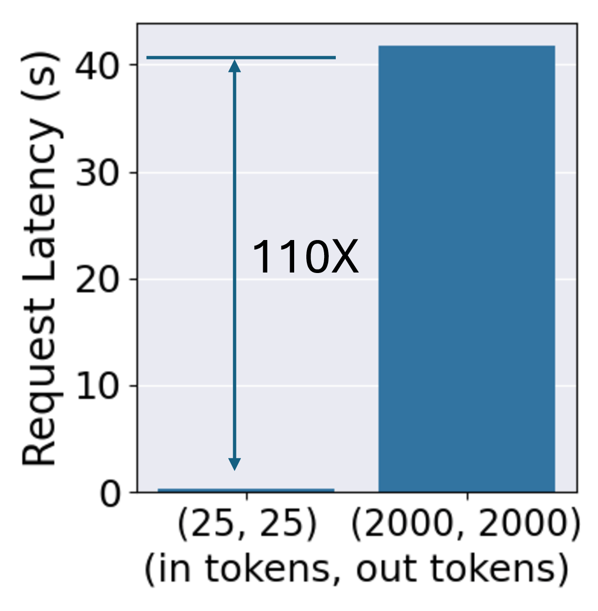
(a) LLaMA-7B

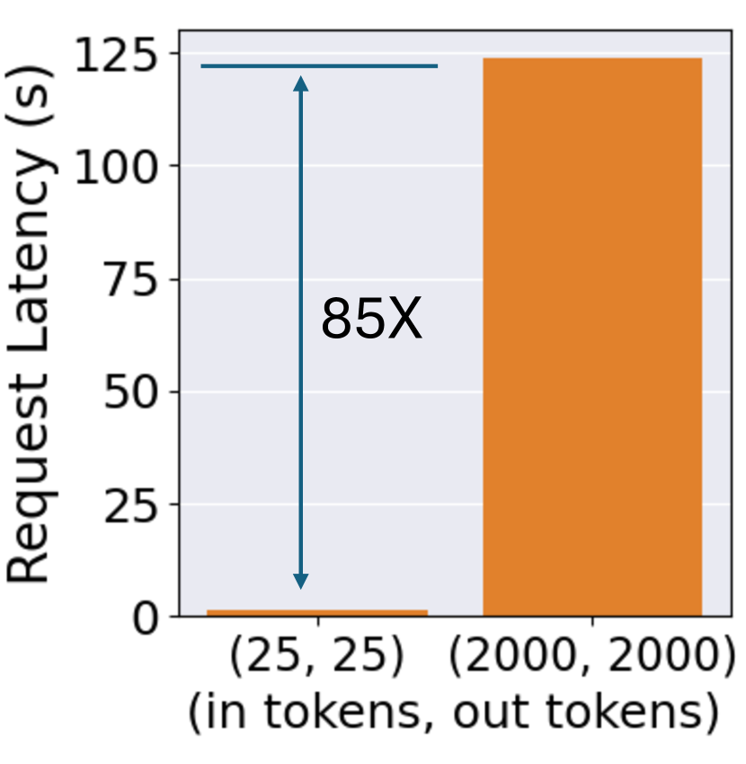
(b) LLaMA-70B

Figure 1: Request latency of different input/output lengths on A100-80G.

Unlike traditional machine learning workloads, LLM tasks exhibit significant variance in request sizes, or input and output lengths. For example, ResNet [16] requires a fixed-dimension input (image size) and results in a fixed-dimension output (classification size). Conversely, transformer-based language models are flexible to support variable-length prompts and produce variable-length generation sequences, as in the Chatbot Arena dataset [53] derived from a real-world LLM chatbot service. Figure 10 illustrates the request size distributions of Chatbot Arena, demonstrating the extensive diversity of request sizes in practical scenarios.

Unsurprisingly, high variance in request sizes introduces significant variation in request latency. As illustrated in Figure 1, request latency can increase by $110\times$ when the input/output length expands from 25 tokens to 2000 tokens for the Llama2-7B model served on an A100 GPU. Consequently, it becomes crucial to recognize that LLM requests, unlike non-transformer models, impose varied loads on GPU resources.

3.2 Unknown Output Length

In most online services, an LLM request’s output length is not known a priori. In this paper, we evaluate GPU cost efficiency based on both input and output lengths. We do this to develop a holistic understanding of GPU cost efficiency, but Mélange’s GPU provisioning decision does not require specific knowledge of the output lengths of individual requests. Instead, it relies only on an estimated distribution of request sizes. We believe it is a fair assumption that a service’s GPU allocator is given a distribution of expected request sizes based on the historical data of previously served input and output lengths.

Because output lengths are a significant contributor to the load of individual requests, unknown output lengths are primarily a challenge for the load balancer, not the allocator. While important, the task of output length prediction for load balancing is orthogonal to Mélange. Therefore, to evaluate the efficacy of Mélange’s GPU allocations, we use a load balancer that assumes knowledge of output lengths. We are actively working to remove this assumption by exploring load balancers based on output length prediction. There are several prior works that perform online LLM output length prediction with high accuracy  [19, 55], but they have not been applied to load balancing. To the best of our knowledge, there is no load balancer that addresses the problem of unknown output lengths, and we believe this to be an promising area of future work.

4 GPU Cost Efficiency Analysis

In this section, we analyze GPU cost efficiency in the context of LLM serving. We first describe our key definitions (§ 4.1), then evaluate the cost efficiency of serving Llama2-7b on two widely used GPUs, NVIDIA’s A100 [34] and A10G [33] to show that GPU cost efficiency is significantly influenced by request size(§ 4.2), request latency SLO(§ 4.3), and request rate(§ 4.4). Finally, we validate the generality of our findings by extending our investigation to include additional hardware, specifically NVIDIA’s H100 and L4 GPUs, and a larger model variant, Llama2-70B (§ 4.5). For clarity, the plots are tagged with the request size, request rate, and SLO used to generate the plot. In each setting, we use vLLM-0.2.7 as the inference engine [21]. Results can differ across versions.

4.1 Definitions

Service-level Objective (SLO). As in prior work [21, 56, 51], we use the average Time Per Output Token (TPOT) as our Service-level Objective (SLO). Average TPOT is determined by dividing total request latency by the number of generated tokens. In general, SLOs are application dependent: in-line code editors (e.g., GitHub Copilot [29]) require tight latency deadlines to suggest real-time code additions, whereas text summarization services may permit additional processing time to generate concise and accurate summaries for large documents. There are other popular definitions of SLO, such as time to first token and total request latency. To simplify our discussion, we use only TPOT, however, Mélange is flexible to support alternative definitions of SLO.

Cost Efficiency Metric. We use tokens per dollar (T/$) to measure GPU cost efficiency, which is calculated by summing input and output token lengths served within some time period, and dividing the sum by the GPU’s rental cost for the same period. The resulting value enables us to directly compare cost efficiency across GPU instance types with different rental costs. Pricing inference based on token lengths is a common practice in LLM services [36, 12], but some services set different prices for input and output tokens. We only compare T/$ between GPUs in settings where the request sizes are the same, so we do not lose generality to such cost models. In settings where request sizes differ, we report the overall cost of the GPU allocation that meets the aggregate workload. In general, we derive T/$ based on profiling a GPU at maximum saturation. When an SLO is specified, T/$ is calculated by finding the highest GPU saturation at which average TPOT still meets the SLO requirement.

4.2 Request Size and Cost Efficiency

We now show that request sizes, shown to be widely varying (§ 3.1), dramatically affect GPU cost efficiency. We served Llama2-7b on A100 and A10G (specifications reported in Table 1), and derived each GPU’s T/$ at maximum GPU saturation across a range of request sizes, with results in Figure 2(a). Interestingly, neither GPU achieves highest T/$ across the entire request size space. Instead, each GPU achieves greater cost efficiency within distinct regions of the request size spectrum. For smaller request sizes, A10G exhibits up to $2.6\times$ greater T/$ than A100. Conversely, for larger request sizes, A100 achieves up to $1.5\times$ the cost efficiency of A10G. We extend this exploration to include both input and output lengths in Figure 2(b) to observe how they affect cost efficiency separately. We find that the two dimensions influence cost efficiency in a similar manner: smaller sizes benefit A10G, and larger sizes are best served on A100. Once again, there exists a clear boundary within the input/output length spectrum where the cost efficiency advantage shifts from A10G to A100 as request sizes increase. In fact, selecting a single GPU type to serve requests across the entire request size space misses opportunities to produce up to 72% more output tokens for the same cost.

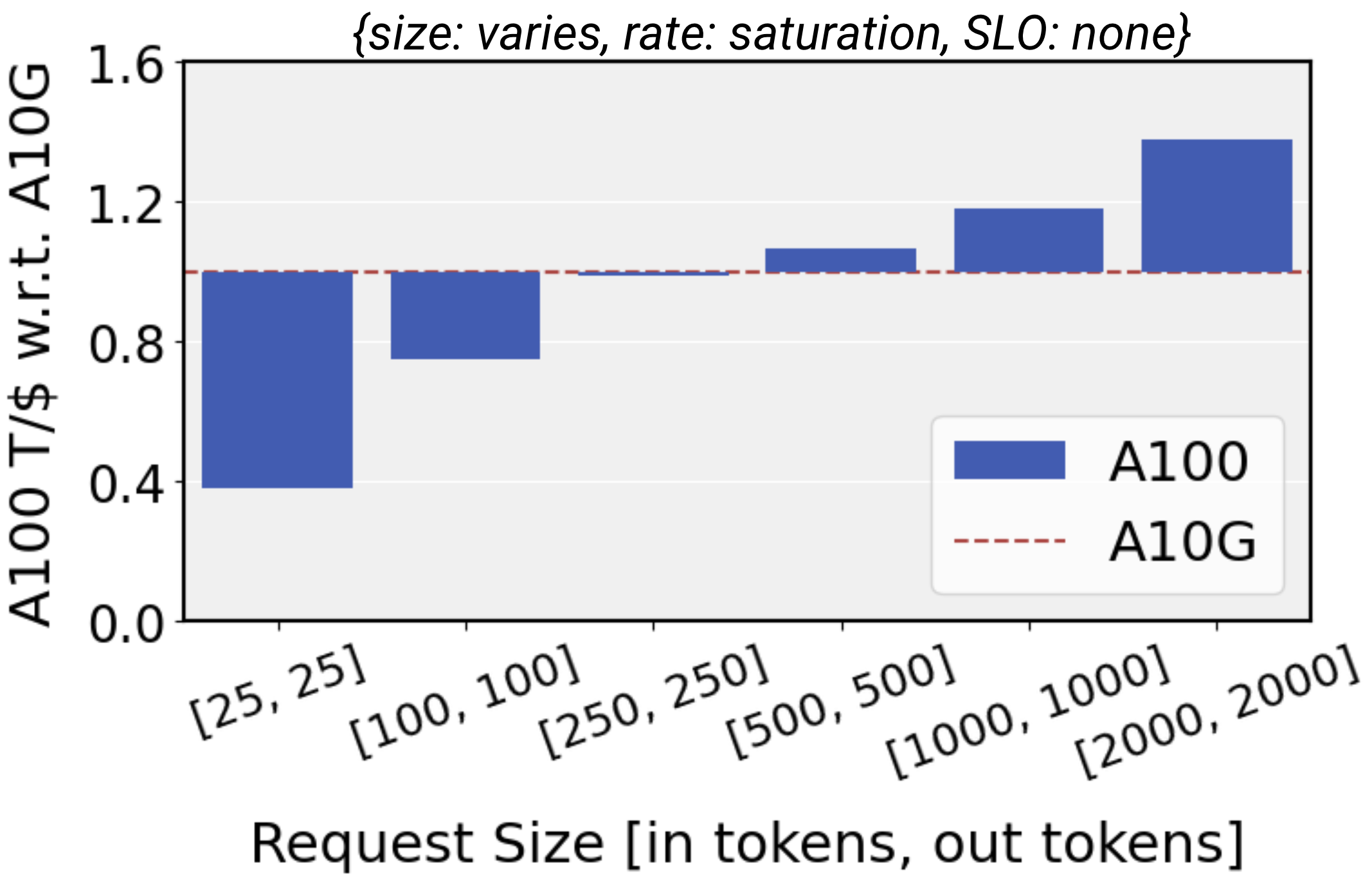
(a) Equivalent input and output lengths

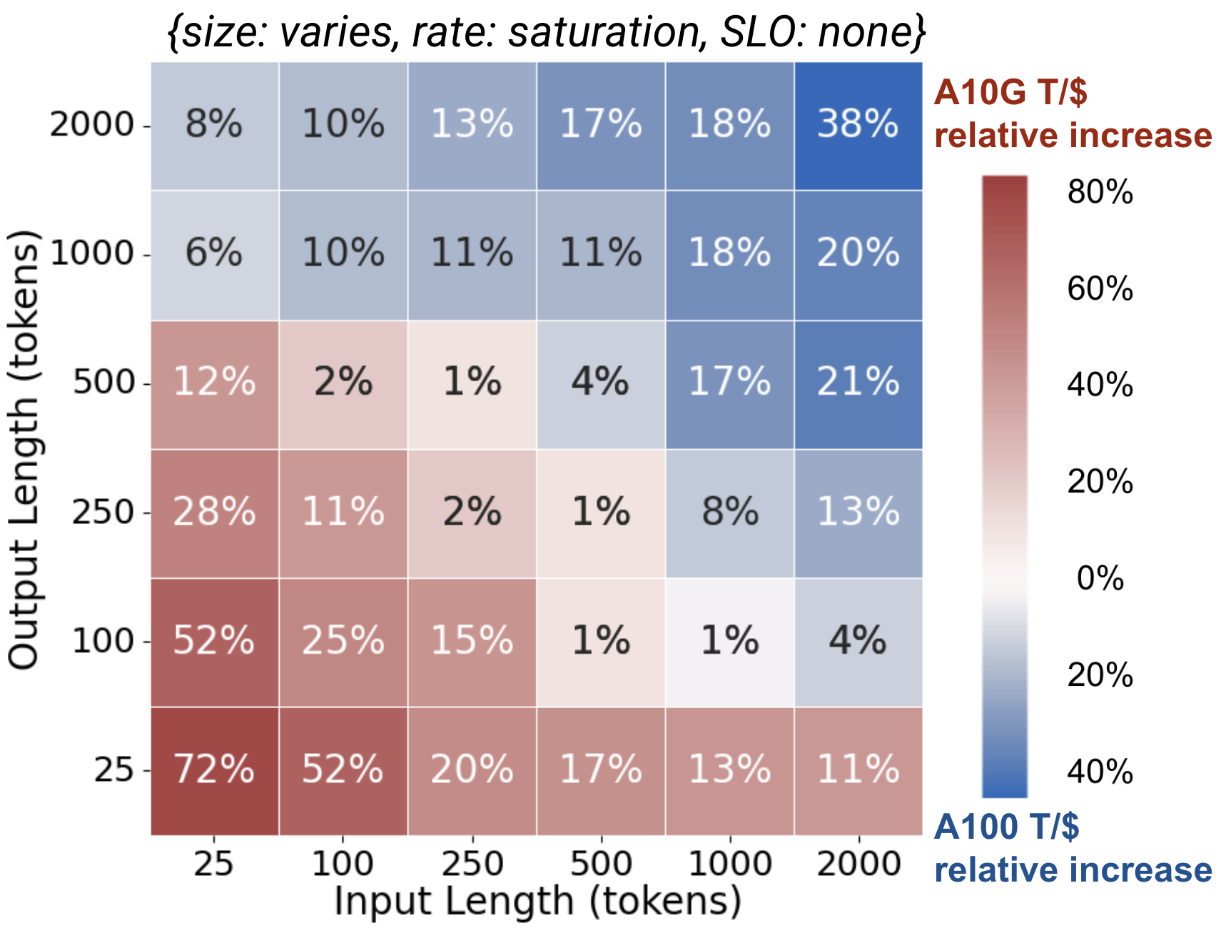
(b) Input and output lengths vary independently

Figure 2: Figure (a) depicts A10G and A100’s relative T/$ across request sizes. Figure (b) expands (a) into separate input and output length dimensions. Tile colors indicate which GPU achieved higher T/$, and values represent the most cost efficient GPU’s percent increase of T/$ relative to the less cost efficient GPU.

Source of Cost Efficiency Variation. Digging deeper into why request size impacts relative cost efficiency between GPUs, we find that it is largely due to the heterogeneity of GPU hardware. Given that batch size directly influences throughput (i.e., request processing rate), we inspect the source of cost efficiency variation by examining the effect of request size on achieved batch size. Figure  3 depicts the absolute batch sizes and batch sizes normalized by instance cost of each GPU at maximum saturation. Note that Figure  3(b) closely resembles Figure  2(a)’s plot of relative T/$ at maximum saturation, verifying that batch size indeed serves as a proxy for throughput.

A10G and A100 have similar dollar-normalized batch sizes at 250 input/output tokens, but as the request size increases to 2000 input/output tokens, A10G’s absolute batch size decreases by a factor of $9\times$ whereas A100’s only decreases by $6\times$ due to its superior memory size and bandwidth. As a result, A100’s cost efficiency advantage over A10G increases accordingly with the increase in request size. In contrast, reducing the request size from 250 to 25 input/output tokens sees A10G’s batch size expanding by $15.2\times$, whereas A100’s growth is more modest at $5.89\times$. We find that this difference is primarily due to the interference of mixing prefill and decode phases of a greater number of requests, as demonstrated in prior work [17]. Because A100’s batch sizes are larger in absolute terms, A100 is more significantly constrained by per-request latency overheads than A10G is. As a result, A10G’s dollar-normalized batch size exceeds A100’s at short request lengths, leading to greater overall T/$ for A10G. This illustrative case demonstrates how the interaction between request size and achieved T/$ can be subtle, and creates a cost efficiency trade-off space among GPU types.

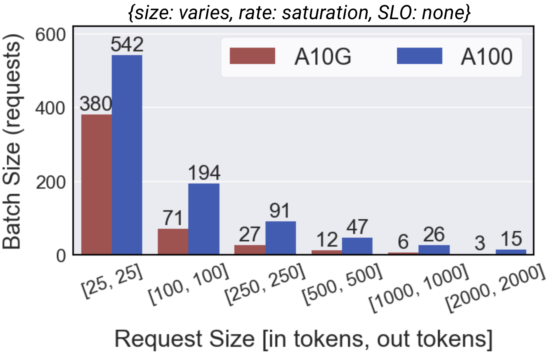
(a) Absolute batch sizes

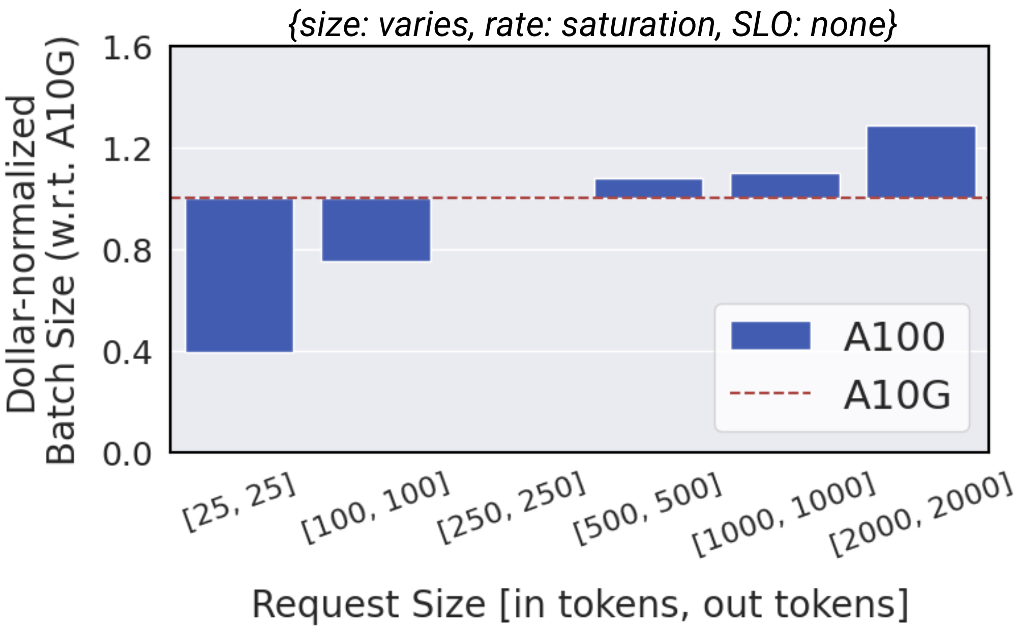
(b) Dollar-normalized batch sizes

Figure 3: (a) depicts the absolute batch sizes of A10G and A100 serving Llama2-7b at maximum saturation, (b) reports the same batch sizes divided by GPU cost, plotting with respect to A10G.

Key Takeaways: GPU cost efficiency is highly dependent on the sizes of requests served. Within the request size space, there are regions where serving with different GPU types is the most cost-effective. In general, lower-end GPUs are more cost-effective for small request sizes whereas higher-end GPUs are best for large request sizes.

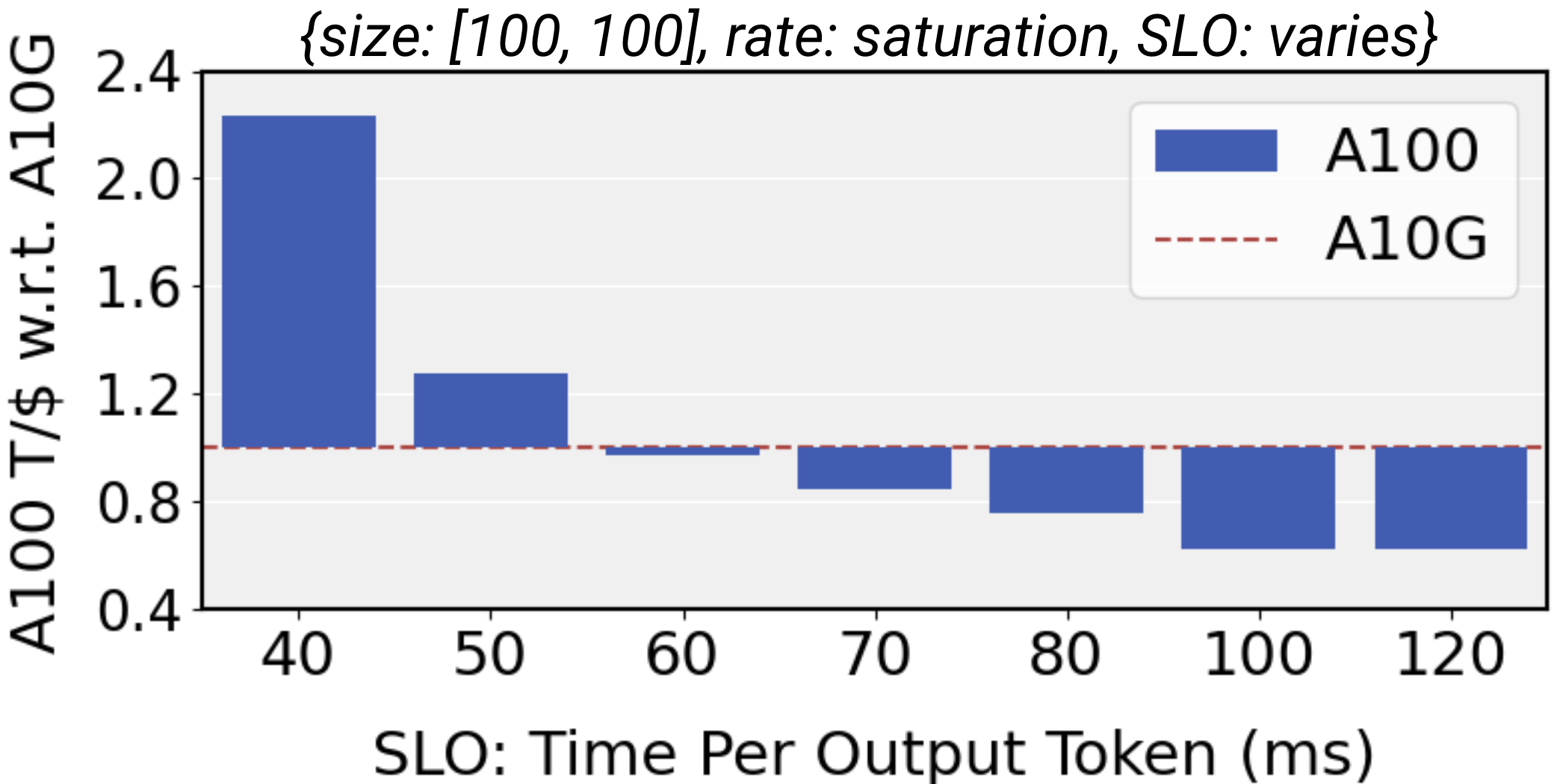
Figure 4: T/$ comparison between A10G and A100 across a range of TPOT SLO parameters.

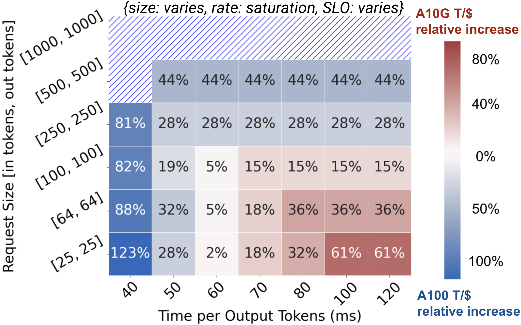
Figure 5: Relative increase in T/$ when combining SLO and request size. Shaded areas indicate regions where A10G fails to satisfy the specified SLO.

4.3 SLO and Cost Efficiency

In this section, we show the impact of SLO on cost efficiency. We measure T/$ by finding the maximum saturation of each GPU while average TPOT remains below SLO, and repeat this across several TPOT deadlines (40ms to 120ms) as shown in Figure 5. Under tight SLO constraints ($<$60ms), A100 demonstrates significantly greater T/$ than A10G ($>2\times$) due to A10G’s higher processing latency, which severely limits its output token rate. However, as the SLO is gradually loosened (60-120ms), A10G’s higher latency is less problematic, dramatically increasing its T/$ and surpassing that of A100 (by $>40\%$). In general, when SLO is stringent, high-end low-latency GPUs are the most viable option because cheaper high-latency GPUs are unable to meet the steep performance requirements. Loosening the SLO increasingly permits the use of cheaper GPUs that can meet the reduced performance requirements at much lower cost.

Further, Figure 5 highlights the interplay between SLO and request size to show that neither can be considered in isolation when determining cost efficiency. Varying the latency SLO adjusts the boundary in the request size space between which different GPU types are more cost effective, and also impacts the degree to which one GPU is more cost effective than the other. For example, with a 40-50ms SLO, A100 always has higher T/$ (by up to $123\%$). At 70ms, A10G shows modest benefit over A100 for small request sizes. And at 100-120ms, A10G demonstrates much greater T/$ advantage over A100 for the same request sizes (up to $61\%$).

Key Takeaways: To comply with strict SLOs, expensive GPUs are often necessary due to the increased latency of cheaper GPUs. However, as SLO is loosened, low-end GPUs can be used to cut deployment costs.

4.4 Request Rate and Cost Efficiency

In this section, we show how request rates influence which GPU, or set of GPUs, is the most cost-effective. Figure 7 illustrates the cost of serving Llama2-7b for a range of request rates using three provisioning strategies: only A10Gs, only A100s, or a mix of both A10Gs and A100s. The y-axis is absolute cost instead of T/$ because each provisioning strategy serves the same request rates and thus the same output tokens; only the cost varies across strategies. As the request rate increases, A100-only is increasingly more cost-effective relative to A10G-only. This is because the requests in this plot were of size [1000 in tokens, 250 out tokens], which § 4.2 shows is more cost effective on A100. However, even in this case, the A10G-only strategy still presents benefits at low request rates ($0-1.5$ req/s). Idle periods of low activity are common in real-world services, and the GPU deployment should right-size to the cheaper GPU (here, A10G) when a higher-end GPU (here, A100) is drastically under-utilized.

Further, a notable finding is that a hybrid deployment approach, combining both A10G and A100 GPUs, yields the greatest cost efficiency. Because A100s have such large capacity, scaling with only A100s is coarse-grained and leads to under-utilized resources. Instead, A10Gs and A100s can be mixed such that A100s satisfy the bulk of the service demands, while A10Gs handle the remaining load at reduced cost.

Key Takeaways: Provisioning a mix of GPU types enables finer-grained resource scaling decisions, which boosts cost efficiency by better utilization of the provisioned instances. At low request rates, LLM deployments should right-size to cheaper low-end GPUs instead of under-utilizing expensive high-capacity GPUs. At higher request rates, a mix of GPU types can be used to better match request load.

4.5 Other Models and Hardware

In this section, we demonstrate the generality of our findings by including additional GPU types and a larger model variant (Llama2-70b) to our analysis. In Figure 8(b), we present relative cost efficiency across four types of GPUs, and observe a progression of the most cost efficient GPU from L4 to A10G, then A100, and finally H100 as the input/output lengths extend. This pattern underscores the advantage of high-end GPUs for processing longer context and output lengths, while low-end GPUs emerge as more cost-effective for shorter input/output scenarios. Similar trends are observed with the Llama2-70B model when comparing the H100 and A100 GPUs, as detailed in Figure 7, reinforcing these insights.

Key Takeaways: The effects of request size on GPU cost efficiency (§ 4.2) generalize to settings with several GPU types and larger model sizes, and similarly leads to significant GPU cost efficiency variations in the request size space.

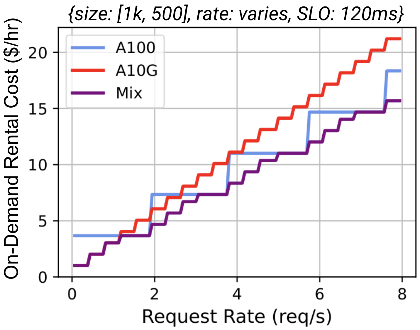
Figure 6: Aggregate GPU hourly rental cost at different request rates. A mix of A100 and A10G consistently achieves the lowest cost.

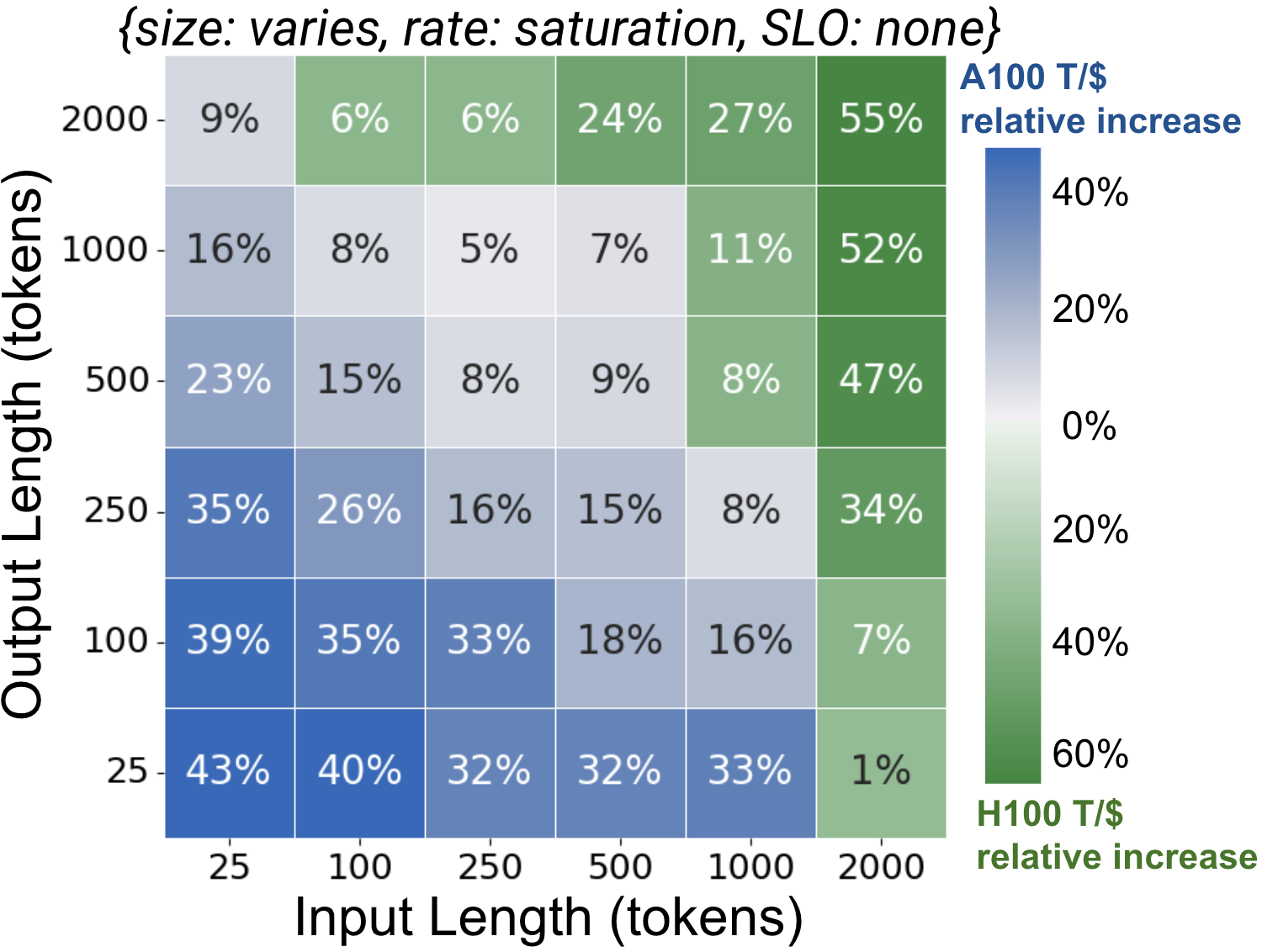
Figure 7: T/$ comparison between H100x2 and A100x2 serving Llama2-70b.

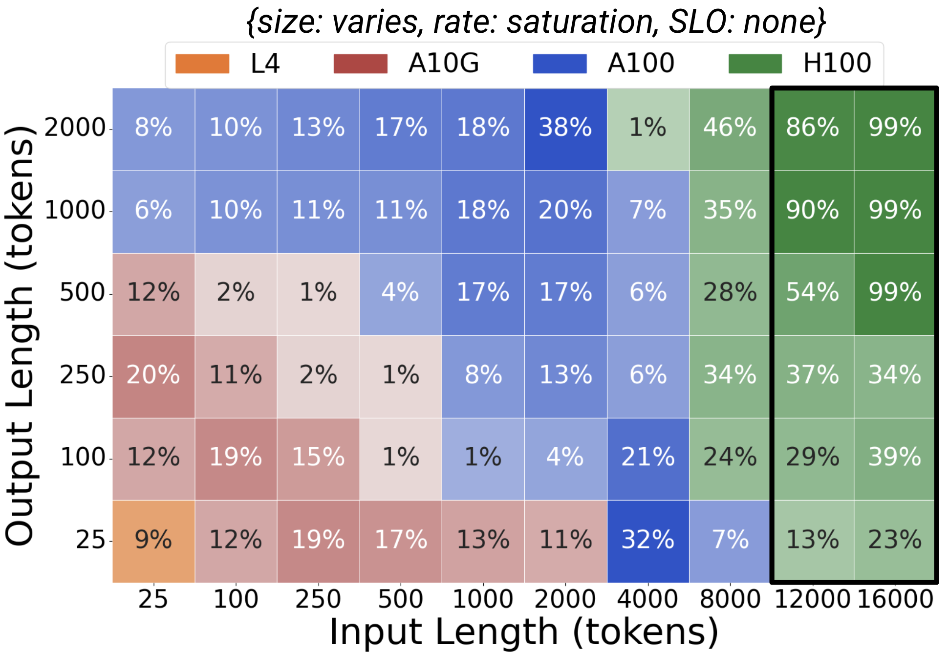
(a) Best GPU relative to second best GPU

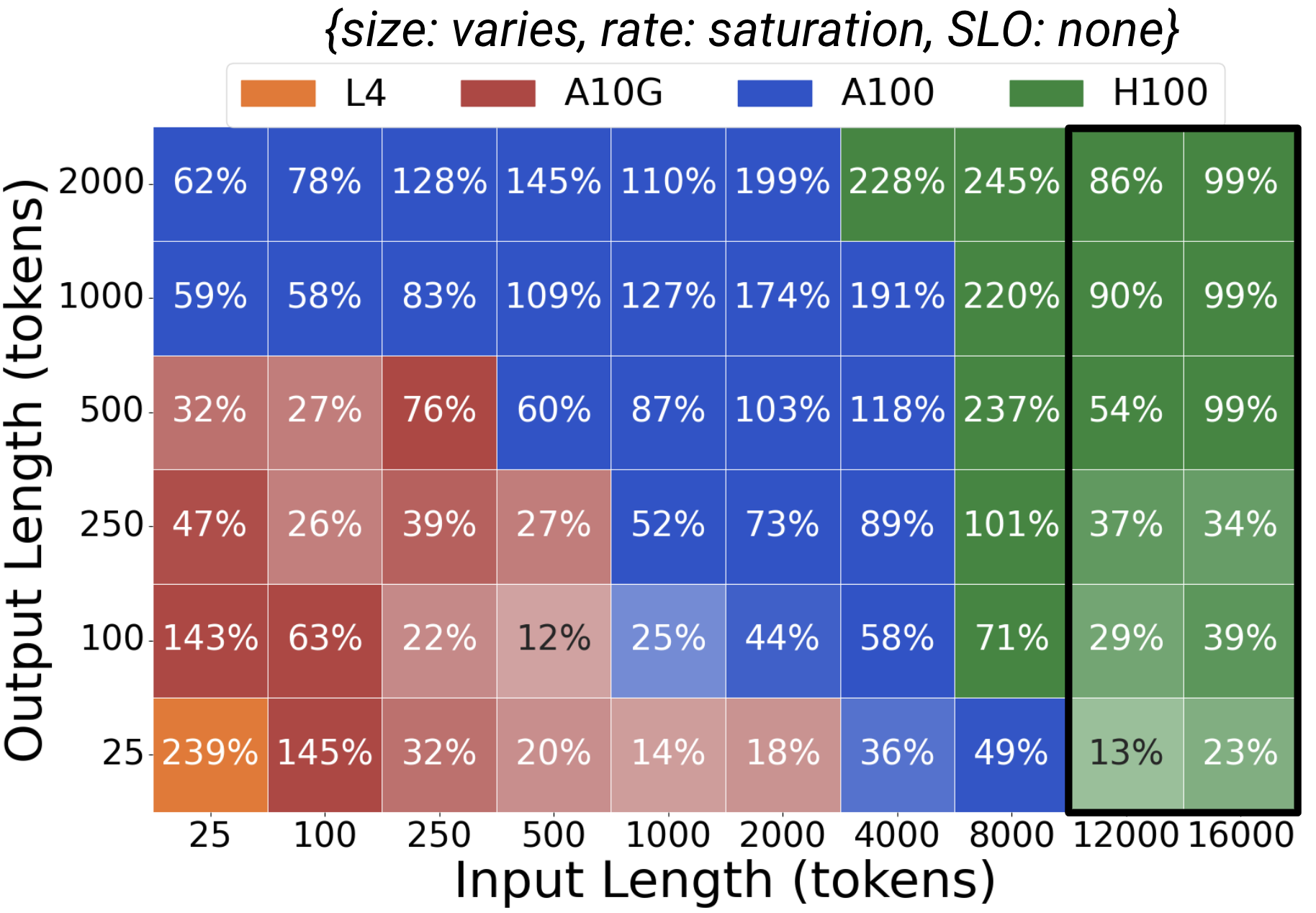
(b) Best GPU relative to worst GPU

Figure 8: Cost efficiency comparison across four GPUs. Tile colors indicate which GPU achieves greatest T/$ at max saturation for the respective request size. Tile values in (a) are the percent increase in T/$ of the best GPU compared to the second best. Tile values in (b) compare the best GPU to the worst GPU. Black boxes indicate request sizes for which only A100 and H100 are compared because A10G and L4 have too small memory capacity to handle a single request within this size, with more detail in § 6.2

.

5 Mélange: Automating Cost-Efficient GPU Selection

Building on the analysis in Section  4, we present Mélange, a framework that automates the selection of GPU instances to meet an LLM service’s demand at minimal cost while adhering to SLO constraints. We frame the GPU selection task as a cost-aware bin-packing problem with GPUs as bins and requests as items, and employ Integer Linear Programming (ILP) to derive the solution.

5.1 Problem Formulation

We begin by defining the key terms utilized in our problem formulation and solution.

Workload: A workload is characterized by its overall request rate along with a distribution of input and output sizes. Given the inherent variability in request sizes, it is crucial to treat the input and output sizes not as fixed values, but as distributions spanning a range of possible lengths. Specifically, as illustrated in Figure 9, a workload is a histogram where each bucket corresponds to a range of request sizes and a bucket’s value is the request rate of requests within the bucket’s size range.

Deployment Cost: Cost is computed by summing the hourly rates for each of the selected instances.

SLO: We use average TPOT to define SLO, however, Mélange can be extended to other definitions of SLO, such as time to first token (TTFT), by profiling maximum T/$ within SLO constraints described in § 4.1 for any given latency constraint definition.

Problem Definition: Given a workload, GPU instance costs, and SLO requirements, our objective is to provision GPUs that can serve the workload at minimal cost while adhering to latency SLO constraints.

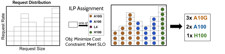
Figure 9: Workflow illustration depicting the process of segmenting request rates into slices, followed by the allocation of hardware resources based on solver recommendations.

5.2 Allocation Algorithm

The intuition of Mélange’s solution is to find the minimal-cost set of GPUs (bins) into which the workload (items) can be bin-packed. To do so, our strategy partitions workload buckets into slices, then assigns the slices to GPUs. Our constraints ensure that the load added to each GPU by the assigned slices does not surpass its maximum capacity. The optimization objective is to reduce the total deployment cost. We discuss bucket size considerations (§ 5.2.1), describe slices in more detail (§ 5.2.2), discuss how load is calculated (§ 5.2.3), then finally detail our ILP formulation (§ 5.2.4).

5.2.1 Request Buckets

As described in § 5.1, a workload is represented by a histogram. The histogram has two dimensions, input length and output length, and each bucket’s value is the aggregate request rate for requests within the bucket’s size range. We make the simplifying assumption that the load (see § 5.2.2) of each request is the same as the largest request size in the same bucket. This simplifies handling diverse request sizes at the cost of over-estimating the load. Bucket sizes can be tuned to reach the desired balance between granularity and solution complexity, but we have not found overall performance to be sensitive to bucket sizes.

5.2.2 Slices

A naive bin-packing of the workload into GPUs is to assign each bucket to a single GPU. However, the overall load of a single bucket may exceed the capacity of a single GPU, and the bucket may be most cost effectively served by splitting across different GPU types. Therefore, for finer-grained bin-packing, buckets are broken down into slices, which are characterized by a request size and rate. A parameter, slice factor, indicates the number of slices that each bucket is divided into. In a setting with a slice factor of 8 and a bucket corresponding to requests of size [$25-100$ in tokens, $25-100$ out tokens] with a request rate of 4 requests/s, the bucket would be segmented into 8 slices each corresponding to a request rate of 0.5 requests.

5.2.3 Load

The ILP solver requires an estimate of the load each slice contributes to a GPU to ensure that the load assigned to an instance does not exceed its capacity and violate the latency SLO. The load of a slice with request size $s$ and rate $r$ on GPU $G$ is calculated as $\frac{r}{MaxTput(G,s,SLO)}$, where $MaxTput(G,s,SLO)$ is the maximum request/s $G$ can achieve for requests of size $s$ while remaining under the latency deadline $SLO$. For instance, if $MaxTput(G,s,SLO)=10\,reqs/s$ and $r=1$, the load is calculated as $1/10=0.1$ or 10%. Each GPU’s maximum capacity is defined as 1 (or 100%). This approximation allows us to calculate the aggregate load of requests with differing sizes and rates. Prior work has proposed cost models for LLM requests  [32, 41], but there is not yet a definitive formulation. We found our simple approximation to perform well, but it can be easily replaced with alternative cost models. Based on offline profiling, we compute $MaxTput(G,s,SLO)$ for each bucket in the workload histogram.

5.2.4 ILP Formulation

We now describe our ILP formulation. We formulate the problem with two primary decision variables. First, let $A$ be a matrix $\{0,1\}^{N\times M}$, where $N$ denotes the total number of slices, and $M$ represents the number of GPU instance types. An element $A_{i,j}$ within this matrix is set to $1$ if slice $i$ is assigned to GPU type $j$, and $0$ otherwise. The second decision variable, $B$, is a vector of length $M$, where each element $B_{j}$ specifies the number of GPUs of type $j$ to be allocated. $c_{j}$ denotes the cost of GPU type $j$ and $r_{i}$ is the request rate of slice $i$. $L$ is computed offline by the process described in § 5.2.3, and element $L_{i,j}$ is the percent load of 1 req/s of slice $i$’s request size on GPU type $j$.

Our objective is to minimize the total GPU allocation cost, with the following mathematical representation:

The ILP constraints are as follows. First, each task slice is assigned to exactly one GPU type:

Second, for each GPU type, the total number of GPUs designated in vector $B$ must adequately accommodate the cumulative load prescribed to it in matrix $A$:

Lastly, the entries within matrix $A$ are binary, and the elements of vector $B$ are non-negative integers:

$$\arg\min_{B}(\sum_{j=1}^{M}B_{j}\cdot c_{j})$$ (1)

$$\forall i\in\{1,\ldots,N\},\quad\sum_{j=1}^{M}A_{i,j}=1$$ (2)

$$\forall j\in\{1,\ldots,M\},\quad\sum_{i=1}^{N}A_{i,j}\cdot L_{i,j}\cdot r_{i}\leq B_{j}$$ (3)

$$\forall i\in\{1,\ldots,N\},\forall j\in\{1,\ldots,M\},\quad A_{i,j}\in\{0,1\}$$ (4)

$$\forall j\in\{1,\ldots,M\},\quad B_{j}\geq 0$$ (5)

Upon resolving equations (1) through (5), the decision variable $B$ holds the minimal-cost set of GPUs that meet the SLO constraint. We use an off-the-shelf solver to solve the ILP problem [30].

6 Evaluation

In this section, we assess the performance of Mélange using four GPU types across settings of diverse request sizes, rates, and SLOs. Our evaluations show that Mélange consistently achieves significant cost savings (up to 77%) compared to single-GPU-type strategies and Mélange’s selected GPU allocations successfully attain TPOT SLO for over 99.5% of requests.

6.1 Methodology

Hardware Setup. We use four NVIDIA GPUs in our evaluations, with specifications detailed in Table 1. To determine GPU cost, we select the lowest on-demand price available from major cloud providers (AWS, Azure, and GCP). Because on-demand H100 is not offered by these major providers, we defer to the pricing from RunPod [40] due to its popularity and availability. To ensure fair cost comparisons, we normalize RunPod’s H100 pricing to match the pricing structures of major platforms. We calculate this by comparing RunPod’s H100 cost ($4.69) to RunPod’s A100-80G cost ($2.29), then adjusting relative to the A100’s price on major clouds ($3.67), resulting in a normalized price of $(4.69/2.29)\times 3.67=\$7.516$ for H100.

Model and Inference Engine. In each experiment, we serve Llama2-7B (Llama-2-7b-hf) [45] using version 0.2.7 of the vLLM inference engine [21] with default parameters.

Mélange Parameters. The bucket ranges correspond to Figure  8(b) and comprise of 10 input length ranges and 6 output length ranges, for a total of 60 buckets. The slice factor is set to 8, for a total of $60\cdot 8=480$ slices.

Datasets. We evaluate across three distinct datasets to cover a wide range of application scenarios. The specific input/output length distributions of these datasets are illustrated in Figure 10.

• Short context: This scenario simulates real-time conversational dynamics by employing the Chatbot Arena dataset (lmsys/lmsys-chat-1m) [53], which is derived from real-world chatbot conversations. The dataset is skewed towards shorter context ($<2000$ tokens) because much of the data was generated in conversation with models that did not yet have a larger context window.

• Long context: This scenario represents tasks with extensive input, such as summarization. We utilize the PubMed dataset (ccdv/pubmed-summarization) [7], comprising 133 thousand scientific papers from PubMed.com, a popular dataset for large-scale text summarization studies.

• Mixed long/short context: This scenario captures settings with a combination of long and short context, such as an assistant that engages in succinct dialogue and responds to large document-based queries. To model this, we create a synthetic dataset by sampling 80% of requests from the Arena dataset and 20% of requests from the PubMed dataset.

SLOs. We referred to current LLM inference benchmarks [3] to set TPOT SLOs, and opted for 40ms in contexts where swift responses are essential, and 120ms where longer response times are acceptable. Both selected SLOs surpass the average human reading speed, ensuring that our SLOs align with practical user experience considerations. However, as discussed in § 4.1, Mélange is flexible to support alternative definitions of SLO.

Baselines. We benchmark against deployments that utilize solely one GPU type. To derive baseline GPU allocations, we use the same ILP formulation from § 5.2.4 but restrict the solver to only a single GPU type.

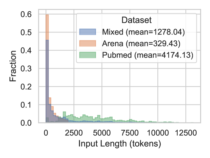
(a) Input length distributions.

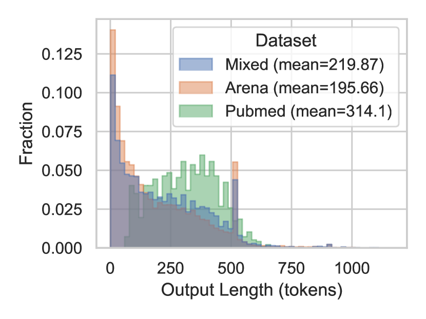
(b) Output length distributions.

Figure 10: Dataset input and output length distributions.

6.2 Cost Savings Analysis

We first compare the overall deployment costs of Mélange’s allocation compared to the single-GPU-type baselines for each dataset and SLO across a range of request rates (1-32 requests/s). Figure 11 displays all costs normalized against the cost of the A100-only strategy (shown in blue dotted lines), and the detailed GPU allocations are included in Appendix A.1. A10G-only and L4-only provisioning strategies are only included in the Arena dataset analysis because of PubMed and Mixed datasets’ large requests. The key-value cache generated from even a single large request ($\sim$12000+ tokens) exceeds the memory capacity of L4 and A10G (24GB). In Mélange’s allocation, L4 and A10G are included but restricted to only serve requests of size less than $12000$ tokens.

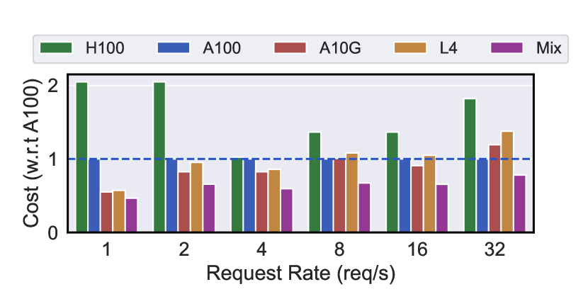
(a) Short context: Arena, SLO = 120ms.

(b) Short context: Arena, SLO = 40ms.

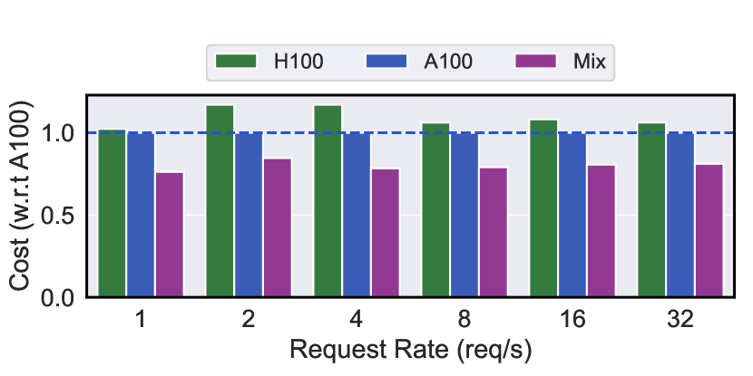
(c) Long context: PubMed, SLO = 120ms.

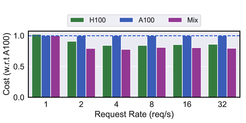
(d) Long context: PubMed, SLO = 40ms.

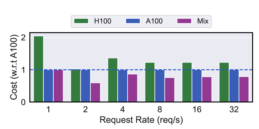
(e) Mixed long/short context, SLO = 120ms.

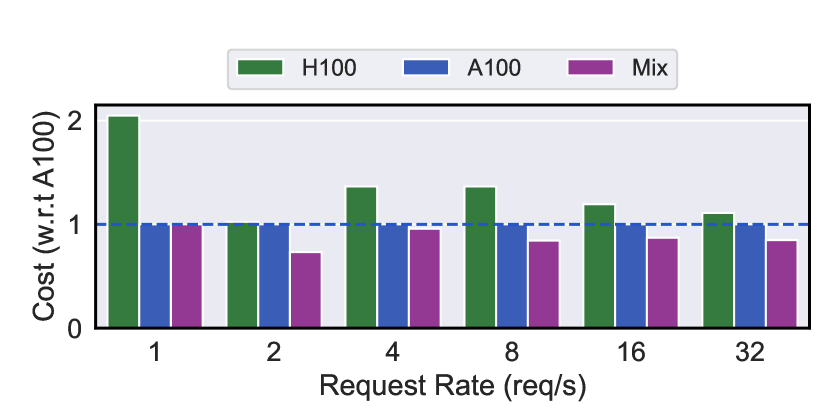
(f) Mixed long/short context, SLO = 40ms.

Figure 11: Deployment cost across different datasets and SLOs.

Loose SLO: 120ms Figures  11(a),  11(c), and  11(e) depict results with a loose 120ms TPOT SLO. Mélange’s mixed-GPU allocation is consistently the most cost-efficient approach, achieving cost reductions of up to 77%, 33% and 51% across the three evaluated datasets.

• Arena Dataset. In Figure 11(a), Mélange achieves 15-77% cost savings. Lower-tier GPUs such as A10G/L4 offer superior cost efficiency in comparison to A100/H100 when handling lower request rates. In particular, for 1-2 requests/s, H100 has egregiously high cost because the load is not enough to even saturate a single GPU. Yet, as request rate increases, A10G/L4’s cost advantage diminishes as high-capacity GPUs become a more reasonable choice. This aligns with findings in § 4.4 that emphasize matching GPU size with request rate. Note, however, that A10G/L4 are still competitive with A100 at higher request rates due to their T/$ advantage for smaller request sizes.

• PubMed Dataset. In Figure 11(c), Mélange achieves 15-33% cost savings. H100’s cost efficiency generally outperforms A100’s, attributable to the dataset’s longer context lengths for which H100 achieves higher T/$. However, there are still many request sizes for which A100 is the best, and this creates the opportunity for the mixed-GPU strategy to squeeze up to 25% cost savings.

• Mixed Dataset. In Figure 11(e), Mélange achieves 13-51% cost savings. A100’s cost efficiency is boosted relative to the PubMed dataset due to it being generally more cost efficient than H100 for small request sizes. This distinction highlights how the nature of the workload — specifically the variance in request lengths — can significantly influence relative cost efficiency across GPU types.

Strict SLO: 40ms Figures  11(b),  11(d), and  11(f) depict the results from tightening the TPOT SLO to 40ms. Once again, Mélange achieves the lowest cost in all settings, with up to 68%, 22%, and 51% reduction across the three evaluated datasets.

• Arena Dataset In Figure 11(b), Mélange achieves 9-68% cost savings. A10G/L4 display considerably higher relative cost than in the loose SLO setting (Figure 11(a)). This is explained by A10G/L4’s higher latency, which requires many more instances to be provisioned in order to meet the tight SLO deadline. Mélange’s mixed-GPU strategy is able to adapt to the strict SLO and provision mostly A100/H100’s which exhibit much lower latencies.

• PubMed Dataset In Figure 11(d), Mélange achieves 2-22% cost savings. H100 achieves a significant cost advantage over A100, especially relative to the 120ms setting ( 11(c)). H100 generally achieves lower latency than A100, making it the preferred option for long-context tight-SLO settings.

• Mixed Dataset In Figure  11(f), Mélange achieves 4-51% cost savings. A100 gains back some advantage over H100 relative to the PubMed setting due to the prevalence of shorter-context requests.

Experiment Takeaways In loose SLO settings, Mélange can utilize all GPU types (both low- and high-end) to serve request sizes for which they achieve greatest T/$ and closely match capacity to the request volume, significantly reducing costs (up to 77%). In tight SLO settings, A10G and L4 are less beneficial due to their high latency, reducing the cost savings Mélange can achieve relative to single-GPU-type strategies. However, even in this setting, Mélange squeezes large cost savings (up to 67%) based on the same principles.

These evaluations highlight the key benefits of exploiting GPU heterogeneity in a unified allocation strategy: 1) GPU types can serve request sizes for which they have greatest T/$, 2) mixing GPU types enables fine-grained provisioning to closely match capacity to request volume, and 3) the allocation strategy can adapt to differing SLO stringency levels and continue to utilize the benefits of (1) and (2). In summary, Mélange efficiently navigates the diversity of request sizes, rates, SLOs, and GPU types to automatically find the best GPU allocation and significantly reduce deployment cost.

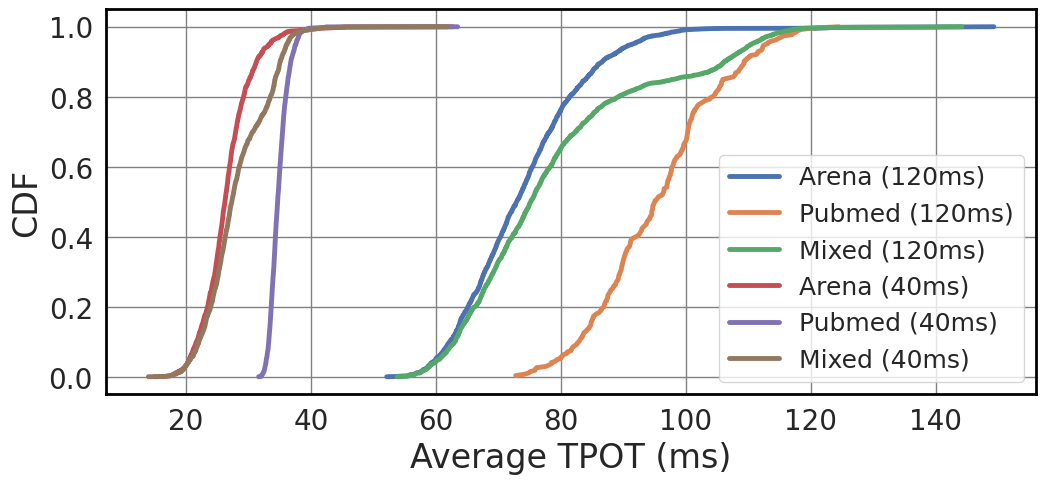
Figure 12: Experiment TPOT CDFs.

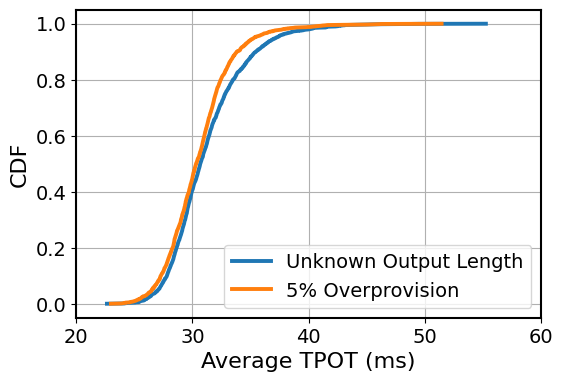
Figure 13: TPOT CDF from unknown output length experiment.

6.3 SLO Satisfaction

Next, we assess Mélange’s ability to select GPU allocations that meet the specified TPOT SLO. To do so, we provision actual cloud GPU instances based on Mélange’s selected allocation for each of the six experiment settings in  6.2 at 4 requests/s. We deploy Llama2-7b with vLLM-0.2.7 on each of the provisioned GPUs. We sample request sizes randomly from the chosen dataset to serve 2000 live requests. We record the latency of each request and divide by output token length to derive average TPOT.

Load Balancer. Most settings use multiple GPU instances, requiring a load balancer to distribute requests across them. The problem of load balancing variable-size requests to heterogeneous backends has been previously explored  [11], and we leave it to future work to create adaptations for serving LLMs on heterogeneous GPUs. We instead use a simple variation of Join Shortest Queue (JSQ) routing [14]: the load balancer tracks outstanding requests for each GPU, and converts them to percent load as described in § 5.2.3. Upon receiving a new request, the load balancer chooses a GPU backend such that the resulting percent load on the chosen GPU is minimized relative to choosing any other GPU. This policy performed well in our experiments, but we expect that improvements to the load balancing policy will reduce tail latency.

Results. Figure 13 presents CDFs of the observed average TPOTs across experiments. With an SLO of 120ms, over 99.95% of requests met SLO. When the SLO was tightened to 40ms, SLO adherence reduced to over 99.5% of requests. Mélange effectively chose GPU allocations that reduce cost while adhering to latency objectives, however, we recognize that services may require even higher SLO adherence, so we investigated the source of SLO violations in our experiment.

SLO Violation Investigation. Of all requests that violated TPOT SLO, we found that 84% failed to meet SLO due to one of two reasons: request rate bursts or co-location with large requests. In our experiments, requests are sent according to a Poisson process, which occasionally creates short-lived bursts that overload the GPU capacity. Further, we choose the size of model request by randomly sampling from the configured dataset. Occasionally, several large requests are chosen in sequence, which can temporarily exceed the service capacity. In an online production environment, it is common practice to over-provision resources in order to absorb such bursts and other load variations. Within our framework, a desired over-provisioning rate (say, 20%) can be achieved by increasing the request rate input to the solver by the same proportion (20%). We discuss the future work of practically deploying a system based on Mélange in § 7.

6.4 Unknown Output Length

As discussed in § 3.2, in order to focus on measuring the quality of Mélange’s chosen GPU allocation, our evaluations utilize a load balancing policy that knows output lengths. Given that this is not a realistic assumption, we briefly evaluate Mélange’s performance with a simple load balancing policy that is unaware of output lengths. We again note that we are actively working on addressing the limitations of unknown output lengths, and believe that LLM-specific load balancing that addresses this challenge is an exciting area for future work. We repeated the SLO satisfaction experiment (§ 6.3) on the Arena dataset with a TPOT SLO of 40ms, but restricted the load balancer to only see request input lengths. The load balancer estimates output length by computing the average of all previous requests’ output lengths. Otherwise, load balancing is performed identically to experiments in § 6.3.

Figure  13 presents the experiment’s TPOT CDF. Only 97.2% of requests met the 40ms deadline, compared to 99.5% in the setting where output length is known, a $5.6\times$ increase in SLO violations. Almost all (91%) of the additional SLO violations were due to large requests landing on a lower-end GPU that would have otherwise landed on a higher-end GPU if the output length was known. This result demonstrates that errors in estimating output length can manifest as increased tail latency due to poor load balancing decisions, further motivating future work on load balancing for LLMs. Nevertheless, we show that over-provisioning can account for the error in predicting output lengths. We re-ran the experiment, but inflated Mélange’s request rate input by 5%, and observed that SLO adherence jumped back up to over 99.5%.

6.5 Solver Time

Request Rate	Arena, SLO=120ms	Arena, SLO=40ms	PubMed, SLO=120ms	PubMed, SLO=40ms	Mix, SLO=120ms	Mix, SLO=40ms
1	0.137	0.177	0.232	0.295	0.168	0.336
2	0.194	0.265	0.234	0.334	0.253	0.381
4	0.192	0.346	0.287	0.381	0.297	0.459
8	0.248	0.433	0.269	0.384	0.321	0.545
16	0.299	0.448	0.389	0.509	0.439	0.537
32	0.316	0.494	0.791	0.96	0.912	1.14

Table 2: Solver execution time.

We present the solver execution time from each experiment in Table 2. Across all datasets and request rates, the solver’s execution time remains under 1.2 seconds, which is negligible compared to workload execution time. We observe a modest increase in solver execution time with higher request volumes, attributed to the greater complexity in slice assignment due to a greater number of required GPUs. However, this increase is sub-linear relative to the increase in request rate, and the solver’s execution time remains practical. Further, the execution of the solver is a one-time event. Users are required to run the solver only prior to deployment or when there is a significant change in the distribution of request sizes or rates.

7 Future Work

There are several interesting directions related to leveraging heterogeneous GPUs for LLM serving. First, adapting heterogeneity-aware load balancing policies specifically for LLM systems where output length is unknown could reduce tail latency that occur due to poor balancing decisions. Further, we believe that generative models beyond LLMs, including image generation, video generation, and embedding models, each of which could be benefited by heterogeneous serving systems. Finally, Mélange effectively derives the best GPU allocation for a fixed workload distribution and request rate, but does not address other challenges of deploying a live LLM service such as handling GPU unavailability or responding to dynamically changing request rate and request size distribution.

8 Conclusion

In this study, we conduct an analysis of GPU cost efficiency in LLM service deployments, and identify three key factors (request sizes, request rates, and Service Level Objectives (SLOs)) that significantly impact GPU cost efficiency. Based on these findings, we introduce Mélange, a framework for deriving the minimal-cost GPU allocation that attains SLO for a given LLM service specification. We frame the task of GPU selection as a cost-aware bin-packing problem and formulate it as an integer linear program. Through evaluations on a range of GPUs, request sizes, request rates, and latency SLOs, Mélange consistently demonstrates significant reductions in deployment costs (up to 77%) while providing high SLO attainment.

Appendix A Appendix

A.1 Instance Allocations

Rate (req/s)	Solver	L4	A10G	A100	H100	Norm. Cost ($/hr)	Savings
1	Mix	1	1			1.71	N/A
	H100-only				1	7.516	77.25%
	A100-only			1		3.67	53.41%
	A10G-only		2			2.02	15.35%
	L4-only	3				2.1	18.57%
2	Mix	2	1			2.41	N/A
	H100-only				1	7.516	67.94%
	A100-only			1		3.67	34.33%
	A10G-only		3			3.03	20.46%
	L4-only	5				3.5	31.14%
4	Mix	1		1		4.37	N/A
	H100-only				1	7.516	41.86%
	A100-only			2		7.34	40.46%
	A10G-only		6			6.06	27.89%
	L4-only	9				6.3	30.63%
8	Mix	1	3	1		7.4	N/A
	H100-only				2	15.032	50.77%
	A100-only			3		11.01	32.79%
	A10G-only		11			11.1	33.39%
	L4-only	17				11.9	37.82%
16	Mix	2	2	3		14.43	N/A
	H100-only				4	30.064	52.00%
	A100-only			6		22.02	34.47%
	A10G-only		20			20.2	28.56%
	L4-only	33				23.1	37.53%
32	Mix	2	6	5		25.81	N/A
	H100-only				8	60.128	57.07%
	A100-only			9		33.03	21.86%
	A10G-only		39			39.39	34.48%
	L4-only	65				45.5	43.27%

Table 3: Instance allocations for the short context Arena dataset, SLO=120ms

Rate (req/s)	Solver	L4	A10G	A100	H100	Norm. Cost ($/hr)	Savings
1	Mix			1	1	11.186	N/A
	H100-only				2	15.032	25.59%
	A100-Only			4		14.68	23.80%
2	Mix		3	1	2	21.732	N/A
	H100-only				4	30.064	27.71%
	A100-Only			7		25.69	15.41%
4	Mix		3	4	3	40.258	N/A
	H100-only				8	60.128	33.05%
	A100-Only			14		51.38	21.65%
8	Mix			7	7	78.302	N/A
	H100-only				14	105.224	25.59%
	A100-Only			27		99.09	20.98%
16	Mix			12	15	156.78	N/A
	H100-only				28	210.448	25.50%
	A100-Only			53		194.51	19.40%
32	Mix	1	1	20	32	315.622	N/A
	H100-only				55	413.38	23.65%
	A100-Only			106		389.02	18.87%

Table 4: Instance allocations for the long context PubMed dataset, SLO=120ms

Rate (req/s)	Solver	L4	A10G	A100	H100	Norm. Cost ($/hr)	Savings
1	Mix			1		3.67	N/A
	H100-only				1	7.516	51.17%
	A100-Only			1		3.67	0%
2	Mix	1		1		4.37	N/A
	H100-only				1	7.516	41.86%
	A100-Only			2		7.34	40.46%
4	Mix		2		1	9.536	N/A
	H100-only				2	15.032	36.56%
	A100-Only			3		11.01	13.39%
8	Mix	1	2	1	1	13.906	N/A
	H100-only				3	22.548	38.33%
	A100-Only			5		18.35	24.22%
16	Mix	1	2	3	2	28.762	N/A
	H100-only				6	45.096	36.22%
	A100-Only			10		36.7	21.63%
32	Mix	1	5	6	4	57.834	N/A
	H100-only				12	90.192	35.88%
	A100-Only			20		73.4	21.21%

Table 5: Instance allocations for the mixed long/short context dataset, SLO=120ms

Rate	Solver	L4	A10G	A100	H100	Norm. Cost ($/hr)	Savings
1	Mix	2	1			2.41	N/A
	H100-only				1	7.516	67.94%
	A100-only			1		3.67	34.33%
	A10G-only		3			3.03	20.46%
	L4-only	5				3.5	31.14%
2	Mix			1		3.67	N/A
	H100-only				1	7.516	51.17%
	A100-only			1		3.67	0.00%
	A10G-only		5			5.05	27.33%
	L4-only	9				6.3	41.75%
4	Mix	1	1	1		5.38	N/A
	H100-only				1	7.516	28.42%
	A100-only			2		7.34	26.70%
	A10G-only		10			10.1	46.73%
	L4-only	17				11.9	54.79%
8	Mix	1	1	2		9.05	N/A
	H100-only				3	15.032	39.80%
	A100-only			3		11.01	17.80%
	A10G-only		16			16.16	44.00%
	L4-only	34				23.8	61.97%
16	Mix		6	3		17.07	N/A
	H100-only				4	30.064	43.22%
	A100-only			6		22.02	22.48%
	A10G-only		40			40.4	57.75%
	L4-only	68				47.6	64.14%
32	Mix		8	6		30.1	N/A
	H100-only				7	52.612	42.79%
	A100-only			9		33.03	8.87%
	A10G-only		80			80.8	62.75%
	L4-only	135				94.5	68.15%

Table 6: Instance allocations for the short context Arena dataset, SLO=40ms

Rate (req/s)	Solver	L4	A10G	A100	H100	Norm. Cost ($/hr)	Savings
1	Mix			4		14.68	N/A
	H100-only				2	15.032	2.34%
	A100-Only			4		14.68	0.00%
2	Mix			1	3	26.218	N/A
	H100-only				4	30.064	12.79%
	A100-Only			9		33.03	20.62%
4	Mix			3	5	48.59	N/A
	H100-only				7	52.612	7.64%
	A100-Only			17		62.39	22.12%
8	Mix			3	12	101.202	N/A
	H100-only				14	105.224	3.82%
	A100-Only			34		124.78	18.90%
16	Mix			11	21	198.206	N/A
	H100-only				28	210.448	5.82%
	A100-Only			67		245.89	19.39%
32	Mix			24	40	388.72	N/A
	H100-only				56	420.896	7.64%
	A100-Only			133		488.11	20.36%

Table 7: Instance allocations for the long context PubMed dataset, SLO=40ms

Rate (req/s)	Solver	L4	A10G	A100	H100	Norm. Cost ($/hr)	Savings
1	Mix			1		3.67	N/A
	H100-only				1	7.516	51.17%
	A100-only			1		3.67	0.00%
2	Mix	1	1	1		5.38	N/A
	H100-only				1	7.516	28.42%
	A100-only			2		7.34	26.70%
4	Mix		3		1	10.546	N/A
	H100-only				2	15.032	29.84%
	A100-only			3		11.01	4.21%
8	Mix	1	3	2	1	18.586	N/A
	H100-only				4	30.064	38.18%
	A100-only			6		22.02	15.59%
16	Mix	2	7	2	3	38.358	N/A
	H100-only				7	52.612	27.09%
	A100-only			12		44.04	12.90%
32	Mix		15	6	5	74.75	N/A
	H100-only				13	97.708	23.50%
	A100-only			24		88.08	15.13%

Table 8: Instance allocations for the mixed long/short context dataset, SLO=40ms

References

- Agrawal et al. [2023] Amey Agrawal, Ashish Panwar, Jayashree Mohan, Nipun Kwatra, Bhargav S Gulavani, and Ramachandran Ramjee. Sarathi: Efficient llm inference by piggybacking decodes with chunked prefills. arXiv preprint arXiv:2308.16369, 2023.
- Ali et al. [2022] Ahsan Ali, Riccardo Pinciroli, Feng Yan, and Evgenia Smirni. Optimizing inference serving on serverless platforms. Proceedings of the VLDB Endowment, 15(10), 2022.
- AnyScale [2024] AnyScale. Anyscale: Llmperf leaderboard. https://github.com/ray-project/llmperf-leaderboard, 2024. [Accessed 13-03-2024].
- AWS [2020] AWS. Ai accelerator-aws trainium. https://aws.amazon.com/machine-learning/trainium/, 2020. [Accessed 14-03-2024].
- Borzunov et al. [2022] Alexander Borzunov, Dmitry Baranchuk, Tim Dettmers, Max Ryabinin, Younes Belkada, Artem Chumachenko, Pavel Samygin, and Colin Raffel. Petals: Collaborative inference and fine-tuning of large models. arXiv preprint arXiv:2209.01188, 2022.
- Chaudhary et al. [2020] Shubham Chaudhary, Ramachandran Ramjee, Muthian Sivathanu, Nipun Kwatra, and Srinidhi Viswanatha. Balancing efficiency and fairness in heterogeneous gpu clusters for deep learning. In Proceedings of the Fifteenth European Conference on Computer Systems, pp. 1–16, 2020.
- Cohan et al. [2018] Arman Cohan, Franck Dernoncourt, Doo Soon Kim, Trung Bui, Seokhwan Kim, Walter Chang, and Nazli Goharian. A discourse-aware attention model for abstractive summarization of long documents. Proceedings of the 2018 Conference of the North American Chapter of the Association for Computational Linguistics: Human Language Technologies, Volume 2 (Short Papers), 2018. doi: 10.18653/v1/n18-2097. URL http://dx.doi.org/10.18653/v1/n18-2097.
- Dao et al. [2022] Tri Dao, Dan Fu, Stefano Ermon, Atri Rudra, and Christopher Ré. Flashattention: Fast and memory-efficient exact attention with io-awareness. Advances in Neural Information Processing Systems, 35:16344–16359, 2022.
- Frantar & Alistarh [2023] Elias Frantar and Dan Alistarh. Sparsegpt: Massive language models can be accurately pruned in one-shot, 2023.
- Frantar et al. [2022] Elias Frantar, Saleh Ashkboos, Torsten Hoefler, and Dan Alistarh. Gptq: Accurate post-training quantization for generative pre-trained transformers. arXiv preprint arXiv:2210.17323, 2022.
- Gandhi et al. [2015] Anshul Gandhi, Xi Zhang, and Naman Mittal. Halo: Heterogeneity-aware load balancing. In 2015 IEEE 23rd International Symposium on Modeling, Analysis, and Simulation of Computer and Telecommunication Systems, pp. 242–251. IEEE, 2015.
- Google [2024] Google. Gemini pricing, 2024. URL https://ai.google.dev/pricing. Accessed: 2024-03-10.
- Gunasekaran et al. [2022] Jashwant Raj Gunasekaran, Cyan Subhra Mishra, Prashanth Thinakaran, Bikash Sharma, Mahmut Taylan Kandemir, and Chita R Das. Cocktail: A multidimensional optimization for model serving in cloud. In 19th USENIX Symposium on Networked Systems Design and Implementation (NSDI 22), pp. 1041–1057, 2022.
- Harchol-Balter [2013] Mor Harchol-Balter. Performance modeling and design of computer systems: queueing theory in action. Cambridge University Press, 2013.
- Harlap et al. [2018] Aaron Harlap, Andrew Chung, Alexey Tumanov, Gregory R Ganger, and Phillip B Gibbons. Tributary: spot-dancing for elastic services with latency SLOs. In 2018 USENIX Annual Technical Conference (USENIX ATC 18), pp. 1–14, 2018.
- He et al. [2015] Kaiming He, Xiangyu Zhang, Shaoqing Ren, and Jian Sun. Deep residual learning for image recognition, 2015.
- Hu et al. [2024] Cunchen Hu, Heyang Huang, Liangliang Xu, Xusheng Chen, Jiang Xu, Shuang Chen, Hao Feng, Chenxi Wang, Sa Wang, Yungang Bao, et al. Inference without interference: Disaggregate llm inference for mixed downstream workloads. arXiv preprint arXiv:2401.11181, 2024.
- Jiang et al. [2023] Youhe Jiang, Ran Yan, Xiaozhe Yao, Beidi Chen, and Binhang Yuan. Hexgen: Generative inference of foundation model over heterogeneous decentralized environment. arXiv preprint arXiv:2311.11514, 2023.
- Jin et al. [2024] Yunho Jin, Chun-Feng Wu, David Brooks, and Gu-Yeon Wei. S3: Increasing gpu utilization during generative inference for higher throughput. Advances in Neural Information Processing Systems, 36, 2024.
- Jouppi et al. [2017] Norman P Jouppi, Cliff Young, Nishant Patil, David Patterson, Gaurav Agrawal, Raminder Bajwa, Sarah Bates, Suresh Bhatia, Nan Boden, Al Borchers, et al. In-datacenter performance analysis of a tensor processing unit. In Proceedings of the 44th annual international symposium on computer architecture, pp. 1–12, 2017.
- Kwon et al. [2023] Woosuk Kwon, Zhuohan Li, Siyuan Zhuang, Ying Sheng, Lianmin Zheng, Cody Hao Yu, Joseph Gonzalez, Hao Zhang, and Ion Stoica. Efficient memory management for large language model serving with pagedattention. In Proceedings of the 29th Symposium on Operating Systems Principles, pp. 611–626, 2023.
- Leviathan et al. [2023] Yaniv Leviathan, Matan Kalman, and Yossi Matias. Fast inference from transformers via speculative decoding. In International Conference on Machine Learning, pp. 19274–19286. PMLR, 2023.
- Lin et al. [2023] Ji Lin, Jiaming Tang, Haotian Tang, Shang Yang, Xingyu Dang, and Song Han. Awq: Activation-aware weight quantization for llm compression and acceleration. arXiv preprint arXiv:2306.00978, 2023.
- Luo et al. [2022] Liang Luo, Peter West, Pratyush Patel, Arvind Krishnamurthy, and Luis Ceze. Srifty: Swift and thrifty distributed neural network training on the cloud. Proceedings of Machine Learning and Systems, 4:833–847, 2022.
- Mehdi [2023] Yusuf Mehdi. Reinventing search with a new ai-powered microsoft bing and edge, your copilot for the web, 2023. URL https://blogs.microsoft.com/blog/2023/02/07/reinventing-search-with-a-new-ai-powered-microsoft-bing-and-edge-your-copilot-for-the-web/. Accessed: 2024-02-21.
- Miao et al. [2022] Xupeng Miao, Yujie Wang, Youhe Jiang, Chunan Shi, Xiaonan Nie, Hailin Zhang, and Bin Cui. Galvatron: Efficient transformer training over multiple gpus using automatic parallelism. arXiv preprint arXiv:2211.13878, 2022.
- Miao et al. [2023a] Xupeng Miao, Chunan Shi, Jiangfei Duan, Xiaoli Xi, Dahua Lin, Bin Cui, and Zhihao Jia. Spotserve: Serving generative large language models on preemptible instances. arXiv preprint arXiv:2311.15566, 2023a.
- Miao et al. [2023b] Xupeng Miao, Yining Shi, Zhi Yang, Bin Cui, and Zhihao Jia. Sdpipe: A semi-decentralized framework for heterogeneity-aware pipeline-parallel training. Proceedings of the VLDB Endowment, 16(9):2354–2363, 2023b.
- Microsoft [2023] Microsoft. Copilot, 2023. URL https://copilot.microsoft.com/. Accessed: 2024-02-21.
- Mitchell [2023] Stuart Mitchell. PuLP: A linear programming toolkit for python. https://github.com/coin-or/pulp, 2023. Accessed: 2024-02-25.
- Narayanan et al. [2020] Deepak Narayanan, Keshav Santhanam, Fiodar Kazhamiaka, Amar Phanishayee, and Matei Zaharia. Heterogeneity-Aware cluster scheduling policies for deep learning workloads. In 14th USENIX Symposium on Operating Systems Design and Implementation (OSDI 20), pp. 481–498, 2020.
- Narayanan et al. [2024] Deepak Narayanan, Keshav Santhanam, Peter Henderson, Rishi Bommasani, Tony Lee, and Percy S Liang. Cheaply estimating inference efficiency metrics for autoregressive transformer models. Advances in Neural Information Processing Systems, 36, 2024.
- Nvidia [2024a] Nvidia. A10 gpu spec, 2024a. URL https://www.nvidia.com/en-us/data-center/products/a10-gpu/. Accessed: 2024-03-10.
- Nvidia [2024b] Nvidia. A100 gpu spec, 2024b. URL https://www.nvidia.com/en-us/data-center/a100/. Accessed: 2024-03-10.
- Nvidia [2024c] Nvidia. Gpus, 2024c. URL https://resources.nvidia.com/l/en-us-gpu. Accessed: 2024-03-10.
- OpenAI [2022] OpenAI. Chatgpt, 2022. URL https://chat.openai.com/. Accessed: 2024-02-21.
- OpenAI [2023] OpenAI. Gpt-4 technical report. arXiv, pp. 2303–08774, 2023.
- Patel et al. [2023] Pratyush Patel, Esha Choukse, Chaojie Zhang, Íñigo Goiri, Aashaka Shah, Saeed Maleki, and Ricardo Bianchini. Splitwise: Efficient generative llm inference using phase splitting. arXiv preprint arXiv:2311.18677, 2023.
- Reid [2023] Elizabeth Reid. Supercharging search with generative ai, 2023. URL https://blog.google/products/search/generative-ai-search/. Accessed: 2024-02-21.
- RunPod [2024] RunPod. Runpod, 2024. URL https://www.runpod.io/console/gpu-cloud. Accessed: 2024-02-24.
- Sheng et al. [2023] Ying Sheng, Shiyi Cao, Dacheng Li, Banghua Zhu, Zhuohan Li, Danyang Zhuo, Joseph E Gonzalez, and Ion Stoica. Fairness in serving large language models. arXiv preprint arXiv:2401.00588, 2023.
- team [2024] FlashInfer team. Accelerating self-attentions for llm serving with flashinfer, 2024. URL https://flashinfer.ai/2024/02/02/introduce-flashinfer.html. Accessed: 2024-02-24.
- Thorpe et al. [2023] John Thorpe, Pengzhan Zhao, Jonathan Eyolfson, Yifan Qiao, Zhihao Jia, Minjia Zhang, Ravi Netravali, and Guoqing Harry Xu. Bamboo: Making preemptible instances resilient for affordable training of large DNNs. In 20th USENIX Symposium on Networked Systems Design and Implementation (NSDI 23), pp. 497–513, 2023.
- Touvron et al. [2023a] Hugo Touvron, Thibaut Lavril, Gautier Izacard, Xavier Martinet, Marie-Anne Lachaux, Timothée Lacroix, Baptiste Rozière, Naman Goyal, Eric Hambro, Faisal Azhar, et al. Llama: Open and efficient foundation language models. arXiv preprint arXiv:2302.13971, 2023a.
- Touvron et al. [2023b] Hugo Touvron, Louis Martin, Kevin Stone, Peter Albert, Amjad Almahairi, Yasmine Babaei, Nikolay Bashlykov, Soumya Batra, Prajjwal Bhargava, Shruti Bhosale, et al. Llama 2: Open foundation and fine-tuned chat models. arXiv preprint arXiv:2307.09288, 2023b.
- Venigalla [2023] Abhi Venigalla. Databricks: Training llms at scale with amd mi250 gpus. https://www.databricks.com/blog/training-llms-scale-amd-mi250-gpus, 2023. [Accessed 14-03-2024].
- Wu et al. [2023a] Bingyang Wu, Yinmin Zhong, Zili Zhang, Gang Huang, Xuanzhe Liu, and Xin Jin. Fast distributed inference serving for large language models. arXiv preprint arXiv:2305.05920, 2023a.
- Wu et al. [2023b] Qingyun Wu, Gagan Bansal, Jieyu Zhang, Yiran Wu, Beibin Li, Erkang Zhu, Li Jiang, Xiaoyun Zhang, Shaokun Zhang, Jiale Liu, Ahmed Hassan Awadallah, Ryen W White, Doug Burger, and Chi Wang. Autogen: Enabling next-gen llm applications via multi-agent conversation, 2023b.
- Wu et al. [2023c] Yiran Wu, Feiran Jia, Shaokun Zhang, Hangyu Li, Erkang Zhu, Yue Wang, Yin Tat Lee, Richard Peng, Qingyun Wu, and Chi Wang. An empirical study on challenging math problem solving with gpt-4. In ArXiv preprint arXiv:2306.01337, 2023c.
- Xiao et al. [2023] Guangxuan Xiao, Ji Lin, Mickael Seznec, Hao Wu, Julien Demouth, and Song Han. Smoothquant: Accurate and efficient post-training quantization for large language models. In International Conference on Machine Learning, pp. 38087–38099. PMLR, 2023.
- Yu et al. [2022] Gyeong-In Yu, Joo Seong Jeong, Geon-Woo Kim, Soojeong Kim, and Byung-Gon Chun. Orca: A distributed serving system for Transformer-Based generative models. In 16th USENIX Symposium on Operating Systems Design and Implementation (OSDI 22), pp. 521–538, 2022.
- Zhang et al. [2019] Chengliang Zhang, Minchen Yu, Wei Wang, and Feng Yan. MArk: Exploiting cloud services for Cost-Effective,SLO-Aware machine learning inference serving. In 2019 USENIX Annual Technical Conference (USENIX ATC 19), pp. 1049–1062, 2019.
- Zheng et al. [2023a] Lianmin Zheng, Wei-Lin Chiang, Ying Sheng, Siyuan Zhuang, Zhanghao Wu, Yonghao Zhuang, Zi Lin, Zhuohan Li, Dacheng Li, Eric. P Xing, Hao Zhang, Joseph E. Gonzalez, and Ion Stoica. Judging llm-as-a-judge with mt-bench and chatbot arena, 2023a.
- Zheng et al. [2023b] Lianmin Zheng, Liangsheng Yin, Zhiqiang Xie, Jeff Huang, Chuyue Sun, Cody Hao Yu, Shiyi Cao, Christos Kozyrakis, Ion Stoica, Joseph E Gonzalez, et al. Efficiently programming large language models using sglang. arXiv preprint arXiv:2312.07104, 2023b.
- Zheng et al. [2024] Zangwei Zheng, Xiaozhe Ren, Fuzhao Xue, Yang Luo, Xin Jiang, and Yang You. Response length perception and sequence scheduling: An llm-empowered llm inference pipeline. Advances in Neural Information Processing Systems, 36, 2024.
- Zhong et al. [2024] Yinmin Zhong, Shengyu Liu, Junda Chen, Jianbo Hu, Yibo Zhu, Xuanzhe Liu, Xin Jin, and Hao Zhang. Distserve: Disaggregating prefill and decoding for goodput-optimized large language model serving. arXiv preprint arXiv:2401.09670, 2024.