Randomized Nyström Preconditioned Interior Point-Proximal Method of Multipliers

Abstract

We present a new algorithm for convex separable quadratic programming (QP) called Nys-IP-PMM, a regularized interior-point solver that uses low-rank structure to accelerate solution of the Newton system. The algorithm combines the interior point proximal method of multipliers (IP-PMM) with the randomized Nyström preconditioned conjugate gradient method as the inner linear system solver. Our algorithm is matrix-free: it accesses the input matrices solely through matrix-vector products, as opposed to methods involving matrix factorization. It works particularly well for separable QP instances with dense constraint matrices. We establish convergence of Nys-IP-PMM. Numerical experiments demonstrate its superior performance in terms of wallclock time compared to previous matrix-free IPM-based approaches.

Key Words.

Regularized interior point methods, preconditioners, matrix-free, randomized Nyström approximation, separable quadratic programming, large-scale optimization

MSC Codes.

90C06, 90C20, 90C51, 65F08

1 Introduction

Solving a large-scale quadratic optimization problem to high precision, such as ${10}^{-6}$ to ${10}^{-8}$ relative accuracy, poses a considerable challenge. First-order methods scale and parallelize well but converge so slowly that accuracy below around ${10}^{-4}$ is generally not achievable. Conversely, interior point methods achieve high accuracy, but are generally only used for problems with $n\leq$10\,000$$ dimensions, as standard implementations require factorization of $n\times n$ matrix at a cost of $O(n^{3})$.

Matrix-free interior point solvers present a solution to this conundrum: these solvers access the original input only through matrix-vector products (matvecs) [22], and so can benefit from algorithmic advances and hardware for fast matrix-vector multiplication. For example, an $n\times n$ discrete Fourier transform (DFT) matrix can be applied to a vector in $O(n\log n)$ time [20, sect. 1.4]; and for general dense matrices, hardware accelerators such as GPUs enable fast matvecs.

Our work aims to solve a primal-dual pair of linearly constrained convex quadratic programs (QPs):

$$\begin{array}[]{rll}\text{(P):}&\underset{x}{\operatorname{\mathrm{minimize}}}&\displaystyle\tfrac{1}{2}x^{T}Qx+c^{T}x\\ &\mathrm{subject}\leavevmode\nobreak\ \mathrm{to}&Ax=b,\\ &&x\geq 0;\end{array}\quad\quad\begin{array}[]{rll}\text{(D):}&\underset{x,y,z}{\operatorname{\mathrm{maximize}}}&\displaystyle b^{T}y-\tfrac{1}{2}x^{T}Qx\\ &\mathrm{subject}\leavevmode\nobreak\ \mathrm{to}&A^{T}y+z=Qx+c,\\ &&y\text{: free},\leavevmode\nobreak\ z\geq 0,\end{array}$$

where $Q\in\mathbb{R}^{n\times n}$ is positive semi-definite, $A\in\mathbb{R}^{m\times n}$, $c$, $x$, and $z\in\mathbb{R}^{n}$, and $b$, $y\in\mathbb{R}^{m}$. We further assume that $Q$ is diagonal throughout this paper, i.e., problem (P) is separable.

This problem template includes many real-world problems. For example, many control problems, ranging from robotics to aeronautics to finance, model the control effort to be minimized as the sum of squares of control inputs (a diagonal quadratic) subject to given initial and final states and to linear dynamics (linear constraints).

Contributions

This work investigates variants of a stabilized interior point framework, the interior point proximal method of multipliers (IP-PMM) [48], for solving separable QPs. These variants use iterative methods to solve the Newton systems that arise as IP-PMM subproblems. We propose to use the randomized Nyström preconditioner [16] to accelerate the iterative solve, and call the resulting algorithm Nys-IP-PMM. We show that Nys-IP-PMM enjoys both numerical stability and faster convergence than other variants of IP-PMM. Nys-IP-PMM solves the Newton system inexactly at each IPM iteration, so it is also an inexact variant of matrix-free IP-PMM. We prove that, for any $\epsilon\in(0,1)$, inexact IP-PMM achieves duality measure $\mu_{k}\leq\epsilon$ after $k=O(n^{4}\log\frac{1}{\epsilon})$ iterations, provided the error in the search direction decreases as $O(\mu_{k})$ (see Theorem 3.1). This result allows us to establish probabilistic convergence results for Nys-IP-PMM (see Theorem 4.1).

In our experiments, we compare the randomized Nyström preconditioner with a more standard choice of preconditioner, the partial Cholesky preconditioner [22, 2, 44], to assess which one improves the performance of IP-PMM the most. We demonstrate that the randomized Nyström preconditioner generally improves the condition number of the normal equations compared to the partial Cholesky preconditioner. The results also demonstrate a significant speed-up in terms of wallclock time when using Nys-IP-PMM compared with using partial Cholesky as the preconditioner in IP-PMM, called Chol-IP-PMM.

Comparison to other variants of IP-PMM

Table 1 summarizes the differences between previous work on IP-PMM and our contributions. The first paper to propose IP-PMM [48] considers QP with exact search direction (i.e., using a direct linear system solver), providing polynomial complexity results and numerical experiments. Numerical performance of inexact IP-PMM on QP has been explored in experimental papers [3, 24] by the same authors along with other researchers. These papers introduce novel preconditioners for the iterative solvers used by inexact IP-PMM, but they use entrywise access to $Q$ and $A$, and so are not matrix-free. However, no theoretical convergence result of inexact IP-PMM on QP is presented. The first theoretical convergence analysis of inexact IP-PMM is established in [49], but on linearly constrained semidefinite programming (SDP), without implementation. In our work, we adapt the convergence proof of inexact IP-PMM for SDP [49] as a theoretical basis for inexact IP-PMM algorithm for solving QP. We propose the randomized Nyström PCG, an iterative matrix-free solver, within inexact IP-PMM and establish probabilistic convergence results, along with numerical experiments to show the efficacy of the method in practice.

Table 1: Features for variants of IP-PMM for convex QP / SDP

	Problem	Search direction	Convergence proof	Matrix-free preconditioning	Numerical results
Pougkakiotis and Gondzio [48]	QP	Exact	✓	-	✓
Bergamaschi et al. [3], Gondzio et al. [24]	QP	Inexact	✗	✗	✓
Pougkakiotis and Gondzio [49]	SDP	Inexact	✓	✗	✗
Nys-IP-PMM (ours)	QP	Inexact	✓	✓	✓

Organization

Section 2 contains an overview of IP-PMM, randomized Nyström preconditioner, and partial Cholesky preconditioner. Section 3 details convergence results for inexact IP-PMM on QP. Section 4 introduces our main algorithm, Nys-IP-PMM, proves convergence of the algorithm, and provides implementation details. Section 5 demonstrates the numerical performance of Nys-IP-PMM.

Notation

For a vector $x\in\mathbb{R}^{n}$, subindex $x_{i}\in\mathbb{R}$ denotes the $i$-th component of $x$, and superindex $x^{k}\in\mathbb{R}^{n}$ denotes the $k$-th iterate. For scalar/matrix, we use subscript $k$ for the iteration count, as usual. Given a set of indices $\mathcal{S}\subset[n]\coloneqq\{1,2,\ldots,n\}$ and an arbitrary vector $x\in\mathbb{R}^{n}$, let $x_{\mathcal{S}}$ denote the sub-vector containing the elements of $x$ wholse indices belong to $\mathcal{S}$. The diagonal matrix with main diagonal $x$ is denoted by $\operatorname{diag}(x)$. We use $\lambda_{i}(M)$ to denote the $i$-th largest eigenvalue of matrix $M$. For a positive definite $M$, we write the $M$-norm $\|u\|_{M}^{2}=u^{T}Mu$. The set of $m\times m$ real symmetric positive semidefinite matrices is denoted by $\mathbb{S}_{+}^{m}(\mathbb{R})$. The $n$-by-$n$ identity matrix is denoted by $I_{n}$ and $\mathbbm{1}_{n}=(1,\ldots,1)^{T}\in\mathbb{R}^{n}$. The cost of computing a matrix-vector product with given matrix $M$ is denoted by $T_{M}$.

2 Background

2.1 Interior-point methods (IPMs)

IPMs are among the most important methods, both in theory and in practice, for solving convex QPs. IPMs were pioneered by the landmark paper of Karmarkar [28] in 1984 on linear programming (LP), with a flurry of activity improving these initial results both in theory [38, 31, 30] and in practice [36, 39, 34, 35]. One key reason for the success of the IPM approach is the use of the logarithmic barrier function [18], a nonlinear programming technique. Later, IPMs were extended to linearly constrained convex QP [27, 60, 40, 19, 42], semidefinite programming (SDP) [57], and more generally conic optimization problems [45, 15, 33]. For a more complete history of IPMs, see the review paper [21].

2.1.1 Regularized IPMs

In primal–dual IPMs for (P) with diagonal $Q$, the majority of the computation is devoted to solving a symmetric positive semi-definite linear system to determine the search direction, $(\Delta x^{k},\Delta y^{k},\Delta z^{k})$, for each iteration $k$. At each iteration, the algorithm forms a new diagonal matrix $\Theta_{k}$ and right-hand side (RHS) vector $\xi^{k}$ and must solve the normal equations

$$A(Q+\Theta_{k}^{-1})^{-1}A^{T}\Delta y^{k}=\xi^{k}.$$ (1)

The system (1), whether solved by direct or iterative methods, is unstable when $A$ is nearly rank-deficient or when $Q+\Theta_{k}^{-1}$ is nearly singular. Regularized IPMs [53, 54, 1, 17] improve stability by regularizing the primal problem (P) and/or dual problem (D). Compared to standard IPMs, regularized IPMs generally require more iterations (linear system solves), but the problem to solve at each iteration is more stable [48]. Regularization is particularly important to matrix-free methods, which must rely on iterative linear system solvers rather than (more stable) direct methods.

2.1.2 Interior point proximal method of multipliers

The first polynomial-time primal-dual regularized IPM is the interior point proximal method of multi -pliers (IP-PMM), proposed by Pougkakiotis and Gondzio [48] in 2021. The algorithm approximately solves a sequence of proximal method of multipliers (PMM) subpro -blems associated with (P)–(D) [51] using an IPM. These PMM subproblems are parametrized by estimates $\zeta^{k}$ and $\lambda^{k}$ of the primal variable $x$ and Lagrange multiplier $y$ respectively, and parameters $\rho_{k}>0$ and $\delta_{k}>0$ controlling the strength of the regularization. The PMM subproblems are quadratic minimization problems:

$$\begin{array}[]{cl}\underset{x\geq 0}{\operatorname{\mathrm{minimize}}}&\displaystyle\frac{1}{2}x^{T}Qx+c^{T}x+(\lambda^{k})^{T}(b-Ax)+\frac{1}{2\delta_{k}}\|Ax-b\|_{2}^{2}+\frac{\rho_{k}}{2}\|x-\zeta^{k}\|^{2}.\end{array}$$ (2)

The linear and quadratic terms $(\lambda^{k})^{T}(b-Ax)+\frac{1}{2\delta_{k}}\|Ax-b\|_{2}^{2}$ are motivated by the method of multipliers (also called the augmented Lagrangian method) [25, 50], and ensure the dual objective is strongly concave. The proximal term $\frac{\rho_{k}}{2}\|x-\zeta^{k}\|^{2}$ provides strong convexity for primal problem and ensures better numerical behavior. When $\rho_{k}=\delta_{k}\rightarrow 0$ and the dual estimate is updated by gradient ascent $\lambda^{k+1}\leftarrow\lambda^{k}-\frac{1}{\delta_{k}}(Ax^{k+1}-b)$, the solution $x^{k}$ to the PMM subproblem (2) converges to the solution to (P) [51].

To solve (2), IPM typically introduces the logarithmic barrier function, enforcing the non-negativity constraint $x\geq 0$, so that the Lagrangian to minimize becomes

$$\mathcal{L}^{\text{IP-PMM}}_{\mu_{k},\rho_{k},\delta_{k}}(x;\zeta^{k},\lambda^{k})=\frac{1}{2}x^{T}Qx+c^{T}x+(\lambda^{k})^{T}(b-Ax)+\frac{1}{2\delta_{k}}\|Ax-b\|_{2}^{2}+\\ +\frac{\rho_{k}}{2}\|x-\zeta^{k}\|^{2}-\mu_{k}\sum_{j=1}^{n}\ln x^{j}.$$ (3)

Introducing the new variables $y=\lambda^{k}-\frac{1}{\delta_{k}}(Ax-b)$ and $z=\mu_{k}\operatorname{diag}(x)^{-1}\mathbbm{1}_{n}$, the first-order optimality conditions for minimizing (3) result in the nonlinear system

$$\begin{bmatrix}c+Qx-A^{T}y-z+\rho_{k}(x-\zeta^{k})\\ Ax+\delta_{k}(y-\lambda^{k})-b\\ \operatorname{diag}(x)z-\mu_{k}\mathbbm{1}_{n}\end{bmatrix}=\begin{bmatrix}0\\ 0\\ 0\end{bmatrix}.$$ (4)

IP-PMM applies a variation of Newton’s method to solve a perturbed form of (4). Specifically, it linearizes the optimality conditions and perturbs the right-hand side (RHS) (see section 3.1 for details and eq. 19 for definitions of $r_{d}^{k}\in\mathbb{R}^{n}$, $r_{p}^{k}\in\mathbb{R}^{m},$ and $r_{\mu}^{k}\in\mathbb{R}^{n}$):

$$\begin{bmatrix}-\left(Q+\rho_{k}I_{n}\right)&A^{T}&I_{n}\\ A&\delta_{k}I_{m}&0\\ \operatorname{diag}(z^{k})&0&\operatorname{diag}(x^{k})\end{bmatrix}\begin{bmatrix}\Delta x^{k}\\ \Delta y^{k}\\ \Delta z^{k}\end{bmatrix}=\begin{bmatrix}r_{d}^{k}\\ r_{p}^{k}\\ r_{\mu}^{k}\end{bmatrix}.$$ (5)

When $Q$ is diagonal, by eliminating $\Delta x^{k}$ and $\Delta z^{k}$ using the first and third block of equations in (5), the Newton system (5) can be reduced to solving (6) and computing $\Delta x^{k}$ and $\Delta z^{k}$ via (7)–(8)

$$(N_{k}+\delta_{k}I_{m})\Delta y^{k}=\xi^{k};$$ (6)

$$\Delta x^{k}=(Q+\Theta_{k}^{-1}+\rho_{k}I_{n})^{-1}(A^{T}\Delta y^{k}-r_{d}^{k}+\operatorname{diag}(x^{k})^{-1}r_{\mu}^{k});$$ (7)

$$\Delta z^{k}=\operatorname{diag}(x^{k})^{-1}(r_{\mu}^{k}-\operatorname{diag}(z^{k})\Delta x^{k}),$$ (8)

where $N_{k}\coloneqq A(Q+\Theta_{k}^{-1}+\rho_{k}I)^{-1}A^{T}$, $\Theta_{k}=\operatorname{diag}(x^{k})\operatorname{diag}(z^{k})^{-1}$ is diagonal, and

$$\xi^{k}=r_{p}^{k}+A(Q+\Theta_{k}^{-1}+\rho_{k}I_{n})^{-1}(r_{d}^{k}-\operatorname{diag}(x^{k})^{-1}r_{\mu}^{k}).$$

Equation (6) is the regularized version of normal equations (1) in original IPMs and is solved to determine the search direction of IP-PMM.

The polynomial complexity results of IP-PMM are built upon the choice $\rho_{k}=\delta_{k}=\mu_{k}$. That is, the convergence theory for IP-PMM requires the barrier parameter $\mu_{k}=\frac{x_{k}^{T}z_{k}}{n}$ to control both the IPM and the proximal method. Under this choice and standard assumptions, Pougkakiotis and Gondzio [48, Thm. 3] show that every limit point of $\{(x_{k},y_{k},z_{k}):k\in\mathbb{N}\}$ generated by IP-PMM determines a primal-dual solution of pair (P)-(D). They show linear convergence of the method: for any given tolerance error $\epsilon\in(0,1)$, IP-PMM produces a sequence of iterates $\{(x_{k},y_{k},z_{k})\}_{k\in\mathbb{N}}$ such that $\mu_{k}\leq\epsilon$ after $O(n^{4}\log\frac{1}{\epsilon})$ iterations [48, Thm. 2]. Their results assume the Newton system (5) is solved exactly. While this assumption is reasonable when a direct method solves (6), it becomes untenable when using an iterative method such as CG. We prove convergence for inexact IP-PMM for QP in section 3.

2.2 Preconditioned conjugate gradient

The conjugate gradient (CG) method is the most common iterative method to solve (6). However, even with the extra stability conferred by IP-PMM, CG usually stalls, i.e. fails to converge to sufficient accuracy, especially during the final iterations of IP-PMM. Preconditioning is used improve convergence of CG [20, sect. 11.5] by choosing a positive definite matrix $P$, called a preconditioner, replacing the system to be solved with an equivalent symmetric positive definite system:

$$P^{-1/2}(N_{k}+\delta_{k}I_{m})P^{-1/2}v^{k}=P^{-1/2}\xi^{k}$$

with new variable $v^{k}=P^{-1/2}\Delta y^{k}$. The resulting algorithm is called preconditioned conjugate gradient (PCG), and its update relies on the matrix-vector product $v\mapsto P^{-1}v$. Therefore, a good preconditioner has two properties: 1) its inverse $P^{-1}$ must be computationally cheap to apply, and 2) the preconditioned system $P^{-1/2}(N_{k}+\delta_{k}I_{m})P^{-1/2}$ must have a spectrum that allows CG to converge faster than on the original system $N_{k}+\delta_{k}I_{m}$. For example, we may seek a preconditioner so that the preconditioned system has a reduced condition number [26, 7, 11].

2.2.1 Randomized IPMs for linear programming

Many preconditioners in the IPM literature require entrywise access to the matrices $Q$ and $A$ [3, 24, 9, 46, 5, 13, 55, 6]. Among these, the randomized preconditioner by Chowdhury et al. [9] is most related to our work. Chowdhury et al. [9] pioneered the use of randomized preconditioners in non-regularized IPMs for LPs (i.e., $Q=0$) with wide constraint matrix $m\ll n$. In their work, the normal equations take the form $A\Theta_{k}A^{T}\Delta y^{k}=\xi^{k}$. They propose the preconditioner $P=A\Theta_{k}^{-1/2}\Omega\Omega^{T}\Theta_{k}^{-1/2}A^{T}$, where $\Omega\in\mathbb{R}^{n\times\ell}$ is a random sketching matrix such that $P$ approximates $A\Theta_{k}A^{T}$ well in spectral norm with probability at least $1-\eta$ [9, Lemma 2]. The sketch size $\ell$ is of order $\ell=O(m\log(m/\eta))$ and matrix $\Omega$ has $O(\log(m/\eta))$ non-zero entries. As a result, the total computational cost for $P^{-1}$ is $O((\operatorname{nnz}(A)+m^{3})\log(m/\eta))$. The method suffers cubic complexity in the number of constraints $m$.

2.2.2 Partial Cholesky preconditioners

A matrix-free preconditioner offers improved scalability, particularly when entrywise access to $Q$ and $A$ is expensive. Gondzio [22] propose a matrix-free preconditioner in the context of (regularized) IPMs, called the partial Cholesky preconditioner, which is elaborated in Bellavia et al. [2] and Morini [44]. Given a target rank $\ell\ll m$, partial Cholesky forms the greedily pivoted Cholesky factorization $LL^{T}=E(N_{k}+\delta_{k}I)E^{T}$ with appropriate permutation matrix $E\in\mathbb{R}^{m\times m}$ and takes the first $\ell$ columns of $L$, $L_{\ell}\in\mathbb{R}^{m\times\ell}$, which corresponds to a rank-$\ell$ approximation $L_{\ell}L_{\ell}^{T}\approx N_{k}+\delta_{k}I$, together with a diagonal matrix that ensures the approximation is positive definite. The key limitation of the partial Cholesky preconditioner lies in its construction, which relies on the entire diagonal of $N_{k}$. Computing the diagonal requires at least $m$ matrix-vector products with $A^{T}$, a computational bottleneck if $A$ is dense.

We describe the partial Cholesky preconditioner in more detail here for completeness, since it is a standard choice for a matrix-free IPM implementation. We omit the iteration count $k$ when it is clear from context. The first $\ell$ columns of the Cholesky factor, $L_{\ell}\coloneqq\begin{bmatrix}L_{11}\\ L_{21}\end{bmatrix}$, yield the following factorization in block form:

$$E(N+\delta I)E^{T}\coloneqq\begin{bmatrix}N_{\delta,11}&N_{\delta,21}^{T}\\ N_{\delta,21}&N_{\delta,22}\end{bmatrix}=\begin{bmatrix}L_{11}&\mathbf{0}\\ L_{21}&I_{m-\ell}\end{bmatrix}\begin{bmatrix}I_{\ell}&\mathbf{0}\\ \mathbf{0}&S\end{bmatrix}\begin{bmatrix}L_{11}^{T}&L_{21}^{T}\\ \mathbf{0}&I_{m-\ell}\end{bmatrix},$$ (9)

where $N_{\delta,11}\in\mathbb{R}^{\ell\times\ell}$ is the leading principal submatrix containing the $\ell$ largest diagonal elements and $S=N_{\delta,22}-N_{\delta,21}N_{\delta,11}^{-1}N_{\delta,21}^{T}$ is the Schur complement of $N_{\delta,11}$. In practice, $S$ is never explicitly formed when performing the Cholesky factorization and hence is not available. The partial Cholesky preconditioner approximates $S$ by its diagonal and takes the form

$$P_{\text{Chol}}=E^{T}\begin{bmatrix}L_{11}&\mathbf{0}\\ L_{21}&I_{m-\ell}\end{bmatrix}\begin{bmatrix}I_{\ell}&\mathbf{0}\\ \mathbf{0}&\operatorname{diag}(S)\end{bmatrix}\begin{bmatrix}L_{11}^{T}&L_{21}^{T}\\ \mathbf{0}&I_{m-\ell}\end{bmatrix}E,$$ (10)

the inverse of which has the closed-form formula

$$P_{\text{Chol}}^{-1}=E^{T}\begin{bmatrix}L_{11}^{-T}&-L_{11}^{-T}L_{21}^{T}\\ \mathbf{0}&I_{m-\ell}\end{bmatrix}\begin{bmatrix}I_{\ell}&\mathbf{0}\\ \mathbf{0}&\operatorname{diag}(S)^{-1}\end{bmatrix}\begin{bmatrix}L_{11}^{-1}&\mathbf{0}\\ -L_{21}L_{11}^{-1}&I_{m-\ell}\end{bmatrix}E.$$ (11)

Pseudocode for the construction of this preconditioner appears in [2, Alg. 1] and [44, Alg. 1–2], while spectral analysis for the preconditioned system is developed in [2, 22]. In our comparison, we construct the partial Cholesky preconditioner by [44, Alg. 2], which yields a more efficient matvec with $P_{\text{Chol}}^{-1}$ when the first $\ell$ columns of $E(N+\delta I)E^{T}$ are more sparse than $L_{11}^{-1}$ and $L_{21}$; and a comparable cost of matvec otherwise [44, sect. 3.1].

Constructing the partial Cholesky preconditioner requires access to the complete diagonal of $N+\delta I$ since we need entry-wise access of $N_{\delta,11}$ for factorization (9) and $\operatorname{diag}(N_{\delta,22})$ for computing $\operatorname{diag}(S)$. Using the form $N=A(Q+\Theta^{-1}+\rho I)^{-1}A^{T}$, the diagonal of $N+\delta I$ can be computed in the following matrix-free manner:

$$r_{i}=(Q+\Theta^{-1}+\rho I)^{-\frac{1}{2}}A^{T}e_{i},\quad(N+\delta I)_{ii}=r_{i}^{T}r_{i}+\delta,\quad\text{for all }i=1,2,\ldots,m.$$

This computation requires $m$ matrix-vector products with $A^{T}$ and componentwise scaling of a length $n$ vector, which costs $O(m(T_{A}+n))$. The diagonal of $S$ can be similarly computed, as a cost $O(m(T_{N_{\delta,21}}+\ell^{2}))$. The total construction cost of partial Cholesky preconditioner is dominated by computing $\operatorname{diag}(N+\delta I)$ and $\operatorname{diag}(S)$, resulting in $O(m(T_{A}+n)+m(T_{N_{\delta,21}}+\ell^{2}))$ arithmetic operations.

2.2.3 Randomized Nyström preconditioners

The randomized Nyström preconditioner is built upon the randomized Nyström low-rank approximation, which we introduce now. Let $N\in\mathbb{S}_{+}^{m}(\mathbb{R})$ be a real symmetric positive semidefinite matrix and $\Omega\in\mathbb{R}^{m\times\ell}$ be a standard random Gaussian test matrix (i.e., each entry is drawn i.i.d. from a standard normal distribution). The integer $\ell\ll m$ is called the sketch size and the matrix $Y=N\Omega\in\mathbb{R}^{m\times\ell}$ is called the sketch of $N$. We observe the sketch can be obtained by $\ell$ matrix-vector products with $N$. The randomized Nyström approximation with respect to the range of $\Omega$ is defined as

$$\hat{N}=(N\Omega)(\Omega^{T}N\Omega)^{+}(N\Omega)^{T}=Y(\Omega^{T}Y)^{+}Y^{T}.$$ (12)

Observe from (12) that this approximation can be constructed directly from the test matrix $\Omega$ and the sketch $Y$, without further access to $N$. The rank of $\hat{N}$ is equal to $\ell$ with probability 1, and hence the terms sketch size and rank are used interchangeably. The formula (12) is not numerically stable. Instead, our algorithm uses [37, Alg. 16] to construct the randomized rank-$\ell$ Nyström approximation. It provides a stable and efficient implementation taking $O(T_{N}\ell+\ell^{2}m)$ arithmetic operations, where $T_{N}$ is the cost of a matvec with $N$. Moreover, [37, Alg. 16] returns the truncated eigendecomposition of the randomized Nyström approximation: $\hat{N}=\hat{U}\hat{\Lambda}\hat{U}^{T}$, where $\hat{U}\in\mathbb{R}^{m\times\ell}$ has orthonormal columns and $\hat{\Lambda}\in\mathbb{R}^{\ell\times\ell}$ is diagonal with diagonal entries $\hat{\lambda}_{1}\geq\cdots\geq\hat{\lambda}_{\ell}$.

Given a rank-$\ell$ randomized Nyström approximation $\hat{N}=\hat{U}\hat{\Lambda}\hat{U}^{T}$, the randomized Nyström preconditioner for regularized system (6) and its inverse take the form

$$P_{\text{Nys}} =\frac{1}{\hat{\lambda}_{\ell}+\delta}\hat{U}(\hat{\Lambda}+\delta I)\hat{U}^{T}+(I-\hat{U}\hat{U}^{T}),$$ (13)

$$P_{\text{Nys}}^{-1} =(\hat{\lambda}_{\ell}+\delta)\hat{U}(\hat{\Lambda}+\delta I)^{-1}\hat{U}^{T}+(I-\hat{U}\hat{U}^{T}).$$ (14)

It is important to highlight that the $m^{2}$ matrix elements of the randomized Nyström preconditioner are not explicitly formed in practice. Instead, $P_{\text{Nys}}$ is viewed as a linear operator defined by $\hat{U}$, $\hat{\Lambda}$, and $\delta$. Algorithm 1 summarizes the procedure.

Algorithm 1 Nyström Preconditioner [16]

1:Positive semidefinite $N_{k}$, sketch size $\ell_{k}$, regularization parameter $\delta_{k}$

2:Inverse of randomized Nyström preconditioner $P_{k}^{-1}$ as a linear operator

3:Compute randomized Nyström rank-$\ell_{k}$ approximation by [37, Alg. 16]:

$$\hat{N}_{k}=\hat{U}\hat{\Lambda}\hat{U}^{T}$$

4:Construct inverse Nyström preconditioner $P_{k}^{-1}$ as in (14) with $\hat{U}$, $\hat{\Lambda}$, and $\delta_{k}$.

In other words, the randomized Nyström preconditioner is directly available once the rank-$\ell$ randomized Nyström approximation has been constructed. Both the Nyström preconditioner and its inverse are cheap to apply: a matvec with either requires $O(m\ell)$ arithmetic operations, dominated by the cost of applying $\hat{U}$ and $\hat{U}^{T}$ to a vector. The required storage for the randomized Nyström preconditioner is $O(m\ell)$. All these properties provide a substantial advantage over partial Cholesky when the target rank $\ell$ is much smaller than $m$; see Table 2.

Table 2: Comparison of randomized Nyström preconditioner and the partial Cholesky preconditioner. The construction cost assumes the matrix of the system takes the form $A(Q+\Theta_{k}+\rho_{k}I)^{-1}A^{T}+\delta_{k}I$.

Preconditioner	Construction Cost	Matvec Cost	Storage
Randomized Nyström	$O(\ell(T_{A}+n)+\ell^{2}m)$	$2\ell m+m+5\ell$	$O(\ell m+\ell)$
Partial Cholesky	$O(m(T_{A}+n)+m(T_{N_{\delta,21}}+\ell^{2}))$	$2\ell m+2m+2\ell^{2}$	$O(\ell m+\ell^{2}+m)$

The randomized Nyström preconditioner can effectively accelerate the convergence of CG on linear systems arising from data-driven models [16, 61]. The reason is that most data matrices usually have rapidly decaying spectra and hence have smaller effective dimension [56, 16, 61, 32]. Given a positive semidefinite matrix $N\in\mathbb{S}_{+}^{m}(\mathbb{R})$ and a regularization parameter $\delta>0$, the effective dimension of $N$ is defined as

$$d_{\text{eff}}(\delta)=\textrm{tr}(N(N+\delta I)^{-1})=\sum_{i=1}^{m}\frac{\lambda_{i}}{\lambda_{i}+\delta},$$ (15)

where $\lambda_{i}$’s are eigenvalues of $N$. The ratio $\lambda_{i}/(\lambda_{i}+\delta)$ is close to $1$ if $\lambda_{i}\gg\delta$; and is close to $0$ if $\lambda_{i}\ll\delta$. As a result, the effective dimension can be understood as a smoothed count of the eigenvalues of $N$ that are greater than or equal to $\delta$. Zhao et al. [61] show that if the sketch size $\ell=O(d_{\text{eff}}(\delta)+\log(\frac{1}{\eta}))$, then with probability at least $1-\eta$, the condition number of the Nyström preconditioned system is bounded by a constant [61, Thm. 4.1], and hence the Nyström preconditioned CG (NysPCG) can achieve $\epsilon$-relative error in $O\left(\log(\frac{1}{\epsilon})\right)$ iterations, independent of the condition number (see Lemma A.3 in appendix).

3 Inexact IP-PMM for convex QP

Pougkakiotis and Gondzio [48] assume the search direction in IP-PMM satisfies the Newton system (5) exactly. This assumption is unrealistic when the inner linear system solver in IP-PMM is iterative. Here, we prove convergence for IP-PMM with errors in the search direction, which we call inexact IP-PMM (see Algorithm 2). Inexact IP-PMM on QP is exactly the same as [48, Alg. IP-PMM], except that in line 7 of Algorithm 2, the inexact version we analyze satisfies the inexact Newton system (see eq. 19 for explicit formula) instead of the exact one. We adopt the assumption $\rho_{k}=\delta_{k}=\mu_{k}$ [48] throughout this section. Section 3.1 introduces some technical definitions, and section 3.2 presents convergence results for inexact IP-PMM.

Algorithm 2 Inexact IP-PMM (adapted from [48, Alg. IP-PMM])

1:QP data $A,Q,b,c$ as in (P), tol

2:$0<\sigma_{\min}\leq\sigma_{\max}\leq 0.5,\leavevmode\nobreak\ C_{N}>0,\leavevmode\nobreak\ 0<\gamma_{\mathcal{A}}<1,\leavevmode\nobreak\ 0<\gamma_{\mu}<1$

3:Set as in (16)

4:Compute infeasibility $r_{p}^{0}\leftarrow Ax^{0}-b$ and $r_{d}^{0}\leftarrow c+Qx^{0}-A^{T}y^{0}-z^{0}$.

5:for $(k=0,1,2,\cdots)$ do

6:     if $\left(\|r_{p}^{k}\|_{2}<\textrm{tol}\right)\wedge\left(\|r_{d}^{k}\|_{2}<\textrm{tol}\right)\wedge\left(\mu_{k}<\textrm{tol}\right)$ then

7:         return $\left(x^{k},y^{k},z^{k}\right)$

8:     else

9:         Choose $\sigma_{k}\in\left[\sigma_{\min},\sigma_{\max}\right]$.

10:         Solve system (19) such that the inexact errors satisfy Assumption 3.1.

11:         Choose largest stepsize $\alpha_{k}\in(0,1]$ such that $\mu_{k}(\alpha)\leq(1-0.01\alpha)\mu_{k}$ and

$${\small\begin{bmatrix}x^{k}+\alpha_{k}\Delta x^{k}\\ y^{k}+\alpha_{k}\Delta y^{k}\\ z^{k}+\alpha_{k}\Delta z^{k}\end{bmatrix}}\in\mathcal{N}_{\mu_{k}(\alpha)}\left(\zeta^{k},\lambda^{k}\right),$$

      where $\mu_{k}(\alpha)=\left(x^{k}+\alpha_{k}\Delta x^{k}\right)^{T}\left(z^{k}+\alpha_{k}\Delta z^{k}\right)/n$.

12:         Update the iterate

$${\small\begin{bmatrix}x^{k+1}\\ y^{k+1}\\ z^{k+1}\end{bmatrix}\leftarrow\begin{bmatrix}x^{k}+\alpha_{k}\Delta x^{k}\\ y^{k}+\alpha_{k}\Delta y^{k}\\ z^{k}+\alpha_{k}\Delta z^{k}\end{bmatrix}}\text{ and }\mu_{k+1}\leftarrow\frac{(x^{k+1})^{T}z^{k+1}}{n}.$$

13:         Set $r_{p}^{k+1}\leftarrow Ax^{k+1}-b$ and $r_{d}^{k+1}\leftarrow c+Qx^{k+1}-A^{T}y^{k+1}-z^{k+1}$.

14:         Set $\tilde{r}_{p}\leftarrow r_{p}^{k+1}-\frac{\mu_{k+1}}{\mu_{0}}\bar{b}$ and $\tilde{r}_{d}\leftarrow r_{d}^{k+1}+\frac{\mu_{k+1}}{\mu_{0}}\bar{c}$.

15:         if $\left((\left\|\left(\tilde{r}_{p},\tilde{r}_{d}\right)\right\|_{2}\leq C_{N}\frac{\mu_{k+1}}{\mu_{0}})\wedge(\left\|\left(\tilde{r}_{p},\tilde{r}_{d}\right)\right\|_{\mathcal{A}}\leq\gamma_{\mathcal{A}}\rho\frac{\mu_{k+1}}{\mu_{0}})\right)$ then

16:              $(\zeta^{k+1},\lambda^{k+1})\leftarrow(x^{k+1},y^{k+1})$

17:         else

18:              $(\zeta^{k+1},\lambda^{k+1})\leftarrow(\zeta^{k},\lambda^{k})$

19:         end if

20:     end if

21:     $k\leftarrow k+1$

22:end for

3.1 Definitions for inexact IP-PMM

In this section, we provide a detail on inexact IP-PMM, including the choice of starting point, neighborhoods, and inexact Newton systems, following [48]. Refer to [48] for more details.

Starting point

For the analysis, we consider starting point $(x^{0},z^{0})=\rho(\mathbbm{1}_{n},\mathbbm{1}_{n})$ for some $\rho>0$ and $y^{0}$ being an arbitrary vector such that $\|y^{0}\|_{\infty}=O(1)$ (i.e., the absolute value of its entries are independent of $n$ and $m$). The initial primal and dual estimates are taken as $\zeta^{0}=x^{0}$ and $\lambda^{0}=y^{0}$, and the initial duality measure is denoted by $\mu_{0}=\frac{(x^{0})^{T}z^{0}}{n}$. In addition, there exist two vectors $\bar{b}$ and $\bar{c}$ such that

$$Ax^{0}=b+\bar{b},\leavevmode\nobreak\ -Qx^{0}+A^{T}y^{0}+z^{0}=c+\bar{c}.$$ (16)

Neighborhoods

IP-PMM is a path-following method that requires each iterate of IP-PMM to lie within a specified neighborhood. The neighborhoods in IP-PMM depend on the parameters in the PMM subproblems (2), as well as the starting point, and are parametrized by $(\zeta^{k},\lambda^{k},\mu_{k})$. IP-PMM uses a semi-norm that depends on the input matrices $A$ and $Q$ to measure primal-dual infeasibility:

$$\|(b,c)\|_{\mathcal{A}}:=\min_{x,y,z}\left\{\|(x,z)\|_{2}:Ax=b,\;-Qx+A^{T}y+z=c\right\}.$$

This norm measures the minimum $2$-norm of $(x,z)$ among all primal-dual feasible tuples $(x,y,z)$ and can be evaluated via QR factorization of $A$ [41, sect. 4]. Now, given the starting point $(x^{0},y^{0},z^{0})$ and vectors $(\bar{b},\bar{c})$ in (16), penalty parameter $\mu_{k}$, and primal-dual estimates $\zeta^{k},\lambda^{k}$, Pougkakiotis and Gondzio [48] define the set

$${\small\tilde{\mathcal{C}}_{\mu_{k}}\left(\zeta^{k},\lambda^{k}\right):=\left\{(x,y,z):\begin{array}[]{c}Ax+\mu_{k}\left(y-\lambda^{k}\right)=b+\frac{\mu_{k}}{\mu_{0}}\left(\bar{b}+\tilde{b}^{k}\right),\\ -Qx+A^{T}y+z-\mu_{k}\left(x-\zeta^{k}\right)=c+\frac{\mu_{k}}{\mu_{0}}\left(\bar{c}+\tilde{c}^{k}\right),\\ \left\|\left(\tilde{b}^{k},\tilde{c}^{k}\right)\right\|_{2}\leq C_{N},\leavevmode\nobreak\ \left\|\left(\tilde{b}^{k},\tilde{c}^{k}\right)\right\|_{\mathcal{A}}\leq\gamma_{\mathcal{A}}\rho\end{array}\right\},}$$ (17)

where $C_{N}>0$ is a constant, $\gamma_{\mathcal{A}}\in(0,1)$, and $\rho>0$ is defined as in the starting point. The vectors $\tilde{b}^{k}$ and $\tilde{c}^{k}$ represent the current scaled (by $\frac{\mu_{0}}{\mu_{k}}$) infeasibility:

$$\tilde{b}^{k} \coloneqq\frac{\mu_{0}}{\mu_{k}}\left(Ax+\mu_{k}\left(y-\lambda^{k}\right)-b-\frac{\mu_{k}}{\mu_{0}}\bar{b}\right),$$

$$\tilde{c}^{k} \coloneqq\frac{\mu_{0}}{\mu_{k}}\left(-Qx+A^{T}y+z-\mu_{k}\left(x-\zeta^{k}\right)-c-\frac{\mu_{k}}{\mu_{0}}\bar{c}\right).$$

The set in (17) contains all points $(x,y,z)$ whose scaled infeasibilities are bounded by a constant in both $\|\cdot\|_{2}$ and $\|\cdot\|_{\mathcal{A}}$. Then the family of neighborhoods is

$$\mathcal{N}_{\mu_{k}}\left(\zeta^{k},\lambda^{k}\right):=\left\{(x,y,z)\in\tilde{\mathcal{C}}_{\mu_{k}}\left(\zeta^{k},\lambda^{k}\right):\begin{array}[]{l}(x,z)>(0,0),\\[1.0pt] x_{i}z_{i}\geq\gamma_{\mu}\mu_{k}\text{ for all }i\end{array}\right\},$$ (18)

where $\gamma_{\mu}\in(0,1)$ is a constant that prevents the component-wise complementarity products from approaching zero faster than $\mu_{k}=(x^{k})^{T}z^{k}/n$.

Inexact Newton system

The search direction $(\Delta x^{k},\Delta y^{k},\Delta z^{k})$ in the inexact IP-PMM solves the following inexact Newton system:

$${\left[\begin{array}[]{ccc}-\left(Q+\mu_{k}I_{n}\right)&A^{T}&I\\ A&\mu_{k}I_{m}&0\\ \operatorname{diag}(z^{k})&0&\operatorname{diag}(x^{k})\end{array}\right]\left[\begin{array}[]{c}\Delta x^{k}\\ \Delta y^{k}\\ \Delta z^{k}\end{array}\right]}\\ =-\left[\begin{array}[]{c}-\left(c+\frac{\sigma_{k}\mu_{k}}{\mu_{0}}\bar{c}\right)-Qx^{k}+A^{T}y^{k}+z^{k}-\sigma_{k}\mu_{k}\left(x^{k}-\zeta^{k}\right)\\ Ax^{k}+\sigma_{k}\mu_{k}\left(y^{k}-\lambda^{k}\right)-\left(b+\frac{\sigma_{k}\mu_{k}}{\mu_{0}}\bar{b}\right)\\ \operatorname{diag}(x^{k})\operatorname{diag}(z^{k})\mathbbm{1}_{n}-\sigma_{k}\mu_{k}\mathbbm{1}_{n}\end{array}\right]+\begin{bmatrix}\varrho_{d}^{k}\\ \varrho_{p}^{k}\\ \varrho_{\mu}^{k}\end{bmatrix},$$ (19)

where the centering parameter $\sigma_{k}\in(0,1)$ is chosen to control how fast the duality measure $\mu_{k}$ must decrease at the next iteration, and $(\varrho_{d}^{k},\varrho_{p}^{k},\varrho_{\mu}^{k})$ model the errors when the system is solved by iterative methods.

3.2 Convergence results of inexact IP-PMM on QP

This section presents convergence results for inexact IP-PMM on QP, a necessary building block for Nys-IP-PMM. We need the following assumption on errors in Newton system (19).

Assumption 3.1.

The errors $(\varrho_{p}^{k},\varrho_{d}^{k},\varrho_{\mu}^{k})$ in inexact Newton system (19) satisfy

$$\varrho_{\mu}^{k}=0,\quad\left\|\left(\varrho_{p}^{k},\varrho_{d}^{k}\right)\right\|_{2}\leq\frac{\sigma_{\min}}{4\mu_{0}}C_{N}\mu_{k},\quad\left\|\left(\varrho_{p}^{k},\varrho_{d}^{k}\right)\right\|_{\mathcal{A}}\leq\frac{\sigma_{\min}}{4\mu_{0}}\gamma_{\mathcal{A}}\rho\mu_{k},$$

where $C_{N},\gamma_{\mathcal{A}}$ are constants defined as in (17), $\sigma_{\min}$ is the lower bound for $\sigma_{k}$ in Algorithm 2, and $\rho$ is determined by the starting point chosen in section 3.1.

The assumption $\varrho_{\mu}^{k}=0$ is reasonable since a practical solution method reduces the Newton system (19) to the augmented system or the normal equations, and recovers $\Delta z^{k}$ using a closed-form formula. The other two assumptions on the inexact errors require that the errors are small whenever the iterate is close to a solution.

We also make the following two standard assumptions to ensure the solution and the problem data are bounded, as in [48, 52].

Assumption 3.2.

The primal-dual QP pair in (P)–(D) has an optimal solution $(x^{*},y^{*},z^{*})$ with $\left\|x^{*}\right\|_{\infty}\leq C^{*},\left\|y^{*}\right\|_{\infty}\leq C^{*}$ and $\left\|z^{*}\right\|_{\infty}\leq C^{*}$, for a constant $C^{*}\geq 0$ independent of $n$ and $m$.

Assumption 3.3.

Let $\eta_{\min}(A)$ (resp. $\eta_{\max}(A)$) denote the minimum (resp. maximum) singular value of $A$ and $\nu_{\max}(Q)$ denote the maximum eigenvalue of $Q$. The constraint matrix of $(\mathrm{P})$ has full row rank $\operatorname{rank}(A)=m$, and there exist constants $C_{\min}>0$, $C_{\max}>0$, $C_{Q}>0$, and $C_{r}>0$, independent of $n$ and $m$, such that $\eta_{\min}(A)\geq C_{\min}$, $\eta_{\max}(A)\leq C_{\max}$, $\nu_{\max}(Q)\leq C_{Q}$, and $\|(c,b)\|_{\infty}\leq C_{r}$.

Theorem 3.1 below provides a polynomial complexity result for inexact IP-PMM, which extends [48, Thm. 2]. The critical analysis lies in Lemmas A.1 and A.2 within Section A.1, which guarantee the existence of a stepsize $\bar{\alpha}=O(\frac{1}{n^{4}})$ at each iteration of inexact IP-PMM.

Theorem 3.1.

Let $\epsilon\in(0,1)$ be a given error tolerance. Choose a starting point as in (16) for inexact IP-PMM such that $\mu_{0}\leq\frac{C}{\epsilon^{\omega}}$ for some positive constants $C$ and $\omega$; and assume the inexact errors in (19) satisfy Assumption 3.1. Given Assumptions 3.2 and 3.3, the iterates $\{(x^{k},y^{k},z^{k})\}_{k\geq 0}$ generated by inexact IP-PMM satisfy $\mu_{k}\leq\epsilon$ after $k=O\left(n^{4}\log\frac{1}{\epsilon}\right)$ iterations.

Proof.

Given Lemma A.2 that guarantees the existence of a stepsize $\bar{\alpha}=O(\frac{1}{n^{4}})$ at each iteration of inexact IP-PMM, the proof follows [48, Thm. 2]. ∎

Remark 1.

Given Lemma A.1 and Lemma A.2 in Section A.1, one can extend [48, Thm. 1] and [48, Thm. 3] to inexact IP-PMM using the parallel argument. The former states that the duality measure $\mu_{k}$ converges $Q$-linearly to zero, and the latter guarantees global convergence to an optimal solution of (P)–(D).

3.3 Errors from the normal equations

When $Q$ is diagonal, the normal equations (6) are solved (inexactly) to determine the search direction, and the other two components, $\Delta x^{k}$ and $\Delta z^{k}$, are obtained (exactly) using the closed-form formula (7)–(8). Denote by $\vartheta^{k}$ the error in the normal equations at the $k$-th iteration:

$$[A(Q+\Theta_{k}^{-1}+\mu_{k}I_{n})^{-1}A^{T}+\mu_{k}I_{m}]\Delta y^{k}=\xi^{k}+\vartheta^{k}.$$ (20)

The next result characterizes how the error $\vartheta^{k}$ in (20) propagates to the Newton system, which will be used in the later analysis for Nys-IP-PMM. The proof is presented in Section A.2.

Proposition 3.1.

Suppose $(\Delta x^{k},\Delta y^{k},\Delta z^{k})$ satisfies eqs. 20, 7 and 8 with $\|\vartheta^{k}\|_{2}\leq C\mu_{k}$ for some constant $C>0$ and $\mu_{k}>0$. Then $(\Delta x^{k},\Delta y^{k},\Delta z^{k})$ satisfies (19) with $(\varrho_{d}^{k},\varrho_{p}^{k},\varrho_{\mu}^{k})=(0,\vartheta^{k},0)$ and the inexact errors satisfy

$$\varrho_{\mu}^{k}=0,\quad\left\|\left(\varrho_{p}^{k},\varrho_{d}^{k}\right)\right\|_{2}\leq C\mu_{k},\quad\left\|\left(\varrho_{p}^{k},\varrho_{d}^{k}\right)\right\|_{\mathcal{A}}\leq C\mu_{k}.$$ (21)

In particular, Assumption 3.1 is fulfilled if

$$C\leq\frac{\sigma_{\min}}{4\mu_{0}}\min\left\{C_{N},\gamma_{\mathcal{A}}\rho\right\}.$$ (22)

Proposition 3.1 says that, if the search direction is obtained through solving the normal equations inexactly and using (7)–(8), then only the second block of Newton system in (19) is inexact. The first and third blocks of equations in Newton system remain exact due to the exact formulas in (7)–(8) for $\Delta x^{k}$ and $\Delta z^{k}$.

4 Nyström preconditioned IP-PMM (Nys-IP-PMM)

We introduce our main algorithm: Nyström preconditioned IP-PMM (Nys-IP-PMM) in this section. Given the assumption that $Q$ in (P)–(D) is diagonal, Nys-IP-PMM uses the Nyström PCG to solve the normal equations (6). Section 4.1 provides a convergence analysis for Nys-IP-PMM, which specifies the preconditioner sketch size $\ell$ required for our convergence theory to hold. We have released a reference implementation of Nys-IP-PMM in Julia [4], discussed in section 4.2.

4.1 Convergence analysis of Nys-IP-PMM

The analysis of inexact IP-PMM in section 3.2 shows that the convergence of inexact IP-PMM requires the inexact errors of Newton system (19) to satisfy the bounds in Assumption 3.1, which hold true if, by Proposition 3.1, NysPCG finds a solution $\Delta y^{k}$ to the inexact normal equations (20) satisfying (22). Indeed, when the sketch size $\ell_{k}$ for Nyström PCG is chosen appropriately, the Nyström PCG can achieve a solution such that $\|\vartheta^{k}\|_{2}\leq C\mu_{k}$, where $C$ satisfies (22), in $O(\log\frac{n}{\mu_{k}})$ PCG iterations with high probability (see Lemma A.4 for the rigorous statement). Hence we establish the following convergence results for Nys-IP-PMM. The proof appears in Section A.3.

Theorem 4.1.

Let $\epsilon\in(0,1)$ be a given error tolerance. Instate the assumptions of Theorem 3.1 and suppose the sketch size in Nys-IP-PMM is taken to be

$$\ell_{k}\geq 8\left(\sqrt{d_{\text{eff}}(\mu_{k})}+\sqrt{32\log(16(k+2))}\right)^{2}.$$ (23)

Then,

1. with probability at least 0.9, Nyström PCG runs at most $O\left(\log\frac{n}{\epsilon}\right)$ iterations in each Nys-IP-PMM iteration;

2. after $k=O(n^{4}\log(\frac{1}{\epsilon}))$ Nys-IP-PMM iterations, the duality measure satisfies $\mu_{k}\leq\epsilon$.

Hence, the total number of matvecs with $A$ required is at most $O\left(n^{4}\log(\frac{1}{\epsilon})\log(\frac{n}{\epsilon})\right)$.

The sketch size $\ell^{k}$ in Theorem 4.1 grows with $k$ to ensure the number of inner iterations of PCG is sublinear in $n$. In any given iteration, if $\ell^{k}$ is chosen smaller than the bound (23), item 1) above may fail, but item 2) still holds: in particular, Nys-IP-PMM is still guaranteed to converge. Our practical observations in section 5 indicate that a fixed sketch size typically performs well.

4.2 Implementation of Nys-IP-PMM

Many implementation details deviate slightly from the theory to improve performance, following [48]; see supplement for details. Pseudocode for Nys-IP-PMM appears in Algorithm 3.

Algorithm 3 Randomized Nyström Preconditioned IP-PMM (Nys-IP-PMM)

1:QP data $A$, $b$, $c$, $u$ as in $(\tilde{\text{P}})$, feasibility and optimality tolerance tol

2:approximate primal-dual solution $(\hat{x},\hat{y},\hat{z},\hat{w},\hat{s})$ to problem $(\tilde{\text{P}})$–$(\tilde{\text{D}})$

3:Compute the initial point $(x^{(0)},y^{(0)},z^{(0)},w^{(0)},s^{(0)})$ as in (57).

4:Set initial PMM subproblem parameters: $\lambda^{(0)}=y^{(0)}$, $\zeta^{(0)}=x^{(0)}$, $\rho_{0}=8$, $\delta_{0}=8$.

5:for $k=0,1,2,\ldots$ do

6:     Check the termination criteria using [48, Alg. TC].

7:     Construct $N_{k}=A(Q+\Theta_{k}^{-1}+\rho_{k}I)^{-1}A^{T}$ as a linear operator.

8:     Choose sketch size $\ell_{k}$.

9:     Construct inverse Nyström preconditioner $P_{k}^{-1}$ by Algorithm 1.

10:     Update the iterate and duality measure by Algorithm 5 with $P_{k}^{-1}$.

11:     Update PMM parameters $\rho_{k}$, $\delta_{k}$, $\lambda^{k}$, $\zeta^{k}$ by [48, Alg. PEU].

12:end for

4.2.1 Free and box-constrained variables

Nys-IP-PMM accepts QPs with free variables and box-constrained variables:

$${\small\begin{array}[]{rll}(\tilde{\text{P}}):&\operatorname{\mathrm{minimize}}&\displaystyle\frac{1}{2}x^{T}Qx+c^{T}x\\ &\mathrm{subject}\leavevmode\nobreak\ \mathrm{to}&Ax=b\\ &&x_{\mathcal{F}}\text{: free},\leavevmode\nobreak\ x_{\mathcal{I}}\geq 0,\\ &&0\leq x_{\mathcal{J}}\leq u_{\mathcal{J}},\end{array}}\leavevmode\nobreak\ {\small\begin{array}[]{rll}(\tilde{\text{D}}):&\operatorname{\mathrm{maximize}}&\displaystyle-\frac{1}{2}x^{T}Qx+b^{T}y-u^{T}s\\ &\mathrm{subject}\leavevmode\nobreak\ \mathrm{to}&-Qx+A^{T}y+z-s=c,\\ &&y\text{:free},\leavevmode\nobreak\ z_{\mathcal{I}\mathcal{J}}\geq 0,s_{\mathcal{J}}\geq 0,\\ &&\end{array}}$$

where $\mathcal{F}$, $\mathcal{I}$, and $\mathcal{J}$ are, respectively, the sets of indices for free variables, non-negative variables, and box-constrained variables; and vector $u_{\mathcal{J}}\in\mathbb{R}^{|\mathcal{J}|}$ denotes the upper bounds. For the ease of presentation, we assumes the vectors $u,z,s$ all have length $n$ and satisfy $u_{\mathcal{I}\cup\mathcal{F}}=0$, $z_{\mathcal{F}}=0$, and $s_{\mathcal{I}\cup\mathcal{F}}=0$; and we use the notation $\mathcal{I}\mathcal{J}=\mathcal{I}\cup\mathcal{J}$ and $\mathcal{I}\mathcal{F}=\mathcal{I}\cup\mathcal{F}$.

It is very important to directly model box-constrained variables, as encoding them as general inequality constraints increases the size of the normal equations from $m+|\mathcal{J}|$ to $m$. Moreover, many practical problems do have bounds on problem variables.

The PMM subproblem to be solved at each Nys-IP-PMM iteration becomes:

$${\small\begin{array}[]{ll}\text{minimize}&\displaystyle\frac{1}{2}x^{T}Qx+c^{T}x+(\lambda^{k})^{T}(b-Ax)+\frac{1}{2\delta_{k}}\|Ax-b\|_{2}^{2}+\frac{\rho_{k}}{2}\|x-\zeta^{k}\|^{2},\\ \text{subject to}&x_{\mathcal{F}}\text{: free},\leavevmode\nobreak\ x_{\mathcal{I}}\geq 0,\leavevmode\nobreak\ 0\leq x_{\mathcal{J}}\leq u_{\mathcal{J}}.\end{array}}$$ (24)

We introduce a logarithmic barrier in the Lagrangian to enforce non-negativity and box constraints: $x_{\mathcal{I}}\geq 0$ and $0\leq x_{\mathcal{J}}\leq u_{\mathcal{J}}$, and derive the corresponding linear system to determine the search direction (analogous to (6)–(8)) in the following five variables: primal variable $x$, Lagrange multiplier $y$ (associated with $Ax=b$), dual variable $z_{\mathcal{I}\mathcal{J}}$ (associated with $x_{\mathcal{I}\mathcal{J}}\geq 0$), slack primal variable $w_{\mathcal{J}}\coloneqq u_{\mathcal{J}}-x_{\mathcal{J}}$, and dual variable $s_{\mathcal{J}}$ (associated with $x_{\mathcal{J}}\geq u_{\mathcal{J}}$). Pseudocode for the search direction appears in Algorithm 4, which takes RHS vectors (explicitly defined later in section 4.2.3), current iterate, current parameters, and preconditioner as input. A detailed derivation for (25)–(29) is available in section B.1.

Algorithm 4 Solve Newton system

1:RHS vectors $r_{p}^{k}$, $r_{d}^{k}$, $r_{u}^{k}$, $r_{xz}^{k}$, $r_{ws}^{k}$; current iterates $x^{k},z^{k},w^{k},s^{k}$; parameters $\rho_{k},\delta_{k}$; inverse preconditioner $P_{k}^{-1}$

2:directions $\Delta x^{k}$, $\Delta y^{k}$, $\Delta z^{k}$, $\Delta w^{k}$, $\Delta s^{k}$ that satisfy (56)

3:Compute the auxiliary vectors $\xi_{\text{au}}^{k}$, $\xi^{k}\in\mathbb{R}^{n}$:

$$\left(\xi_{\text{au}}^{k}\right)_{j}=\begin{cases}0,&\text{if }j\in\mathcal{F};\\ -(x^{k}_{j})^{-1}(r_{xz}^{k})_{j},&\text{if }j\in\mathcal{I};\\ -(x^{k}_{j})^{-1}(r_{xz}^{k})_{j}+(w^{k}_{j})^{-1}(r_{ws}^{k})_{j}-(w^{k}_{j})^{-1}s^{k}_{j}(r_{u})_{j},&\text{if }j\in\mathcal{J},\end{cases}$$

$$\xi^{k}=r_{p}^{k}+A(Q+\Theta_{k}^{-1}+\rho_{k}I)^{-1}(r_{d}^{k}+\xi_{\text{au}}^{k}).$$

4:Use PCG with preconditioner $P_{k}$ to solve $\Delta y^{k}$ from the normal equations:

$$[A(Q+\Theta_{k}^{-1}+\rho_{k}I_{n})^{-1}A^{T}+\delta_{k}I_{m}]\Delta y^{k}=\xi^{k}.$$ (25)

5:Compute $\Delta x^{k}$, $\Delta z^{k}$, $\Delta w^{k}$, $\Delta s^{k}$ from closed-form formulae:

$$\Delta x^{k}=(Q+\Theta_{k}^{-1}+\rho_{k}I)^{-1}(A^{T}\Delta y^{k}-r_{d}^{k}-\xi_{\text{au}}^{k});$$ (26)

$$\Delta w^{k}_{\mathcal{J}}=(r_{u}^{k})_{\mathcal{J}}-\Delta x^{k}_{\mathcal{J}},\quad\Delta w^{k}_{\mathcal{I}\mathcal{F}}=0;$$ (27)

$$\Delta z^{k}_{\mathcal{I}\mathcal{J}}=\operatorname{diag}(x^{k}_{\mathcal{I}\mathcal{J}})^{-1}(r_{xz}^{k})_{\mathcal{I}\mathcal{J}}-\operatorname{diag}(z^{k}_{\mathcal{I}\mathcal{J}})\Delta x^{k}_{\mathcal{I}\mathcal{J}},\quad\Delta z^{k}_{\mathcal{F}}=0;$$ (28)

$$\Delta s^{k}_{\mathcal{J}}=\operatorname{diag}(w^{k}_{\mathcal{J}})^{-1}(r_{ws}^{k})_{\mathcal{J}}-\operatorname{diag}(s^{k}_{\mathcal{J}})\Delta w^{k}_{\mathcal{J}},\quad\Delta s^{k}_{\mathcal{I}\mathcal{F}}=0.$$ (29)

4.2.2 Initial point

Our choice of initial point is inspired by Mehrotra’s initial point [39] and that in [48]. A candidate point is first constructed by ignoring the non-negative constraints and then is modified to ensure the positivity of $x_{\mathcal{I}\mathcal{J}}$, $z_{\mathcal{I}\mathcal{J}}$, $w_{\mathcal{J}}$, $s_{\mathcal{J}}$. See details in section B.2.

Algorithm 5 Predictor-corrector method

1:current iterate $x^{k}$, $y^{k}$, $z^{k}$, $w^{k}$, $s^{k}$; PMM parameters $\lambda^{k}$, $\zeta^{k}$, $\rho_{k}$, $\delta_{k}$; inverse preconditioner $P_{k}^{-1}$

2:new iterate $x^{k+1}$, $y^{k+1}$, $z^{k+1}$, $w^{k+1}$, $s^{k+1}$ and new duality measure $\mu_{k+1}$

3:Compute predictor step $(\Delta_{p}x^{k},\Delta_{p}y^{k},\Delta_{p}z^{k},\Delta_{p}w^{k},\Delta_{p}s^{k})$ by Algorithm 4 with:

$$r_{d}^{k}=c+Qx^{k}-A^{T}y^{k}-z^{k}+s^{k}+\rho_{k}(x^{k}-\zeta^{k}),$$ (30)

$$r_{p}^{k}=b-Ax^{k}-\delta_{k}(y^{k}-\lambda^{k}),$$

$$(r_{u}^{k})_{\mathcal{J}}=u_{\mathcal{J}}-x^{k}_{\mathcal{J}}-w^{k}_{\mathcal{J}},\quad(r_{u}^{k})_{\mathcal{I}\mathcal{F}}=0,$$

$$(r_{xz}^{k})_{\mathcal{I}\mathcal{J}}=-\operatorname{diag}(x^{k}_{\mathcal{I}\mathcal{J}})\operatorname{diag}(z^{k}_{\mathcal{I}\mathcal{J}})\mathbbm{1}_{|\mathcal{I}\mathcal{J}|},\quad(r_{xz}^{k})_{\mathcal{F}}=0,$$

$$(r_{ws}^{k})_{\mathcal{J}}=-\operatorname{diag}(w^{k}_{\mathcal{J}})\operatorname{diag}(s^{k}_{\mathcal{J}})\mathbbm{1}_{|\mathcal{J}|},\quad(r_{ws}^{k})_{\mathcal{I}\mathcal{F}}=0,.$$

4:Find stepsizes $\bar{\alpha}_{p}$ and $\bar{\alpha}_{d}$ for predictor step using (58)–(59).

5:Compute the hypothetical measure for predictor step:

$$\mu_{\text{aff}}=\tfrac{(x^{k}_{\mathcal{I}\mathcal{J}}+\bar{\alpha}_{p}\Delta_{p}x^{k}_{\mathcal{I}\mathcal{J}})^{T}(z^{k}_{\mathcal{I}\mathcal{J}}+\bar{\alpha}_{d}\Delta_{p}z^{k}_{\mathcal{I}\mathcal{J}})+(w^{k}_{\mathcal{J}}+\bar{\alpha}_{p}\Delta_{p}w^{k}_{\mathcal{J}})^{T}(s^{k}_{\mathcal{J}}+\bar{\alpha}_{d}\Delta_{p}s^{k}_{\mathcal{J}})}{|\mathcal{I}\mathcal{J}|+|\mathcal{J}|}.$$ (31)

6:Compute the duality measure $\mu_{k}$ and $\tilde{\mu}^{k}$:

$$\mu_{k}=\frac{\left(x^{k}_{\mathcal{I}\mathcal{J}}\right)^{T}z^{k}_{\mathcal{I}\mathcal{J}}+\left(w^{k}_{\mathcal{J}}\right)^{T}s^{k}_{\mathcal{J}}}{|\mathcal{I}\mathcal{J}|+|\mathcal{J}|},\quad\tilde{\mu}^{k}\coloneqq\frac{\mu_{\text{aff}}^{3}}{\mu_{k}^{2}}.$$

7:Compute corrector step $(\Delta_{c}x^{k},\Delta_{c}y^{k},\Delta_{c}z^{k},\Delta_{c}w^{k},\Delta_{c}s^{k})$ by Algorithm 4 with:

$$r_{d}^{k}=0,\quad r_{p}^{k}=0,\quad(r_{u}^{k})_{\mathcal{J}}=0,$$ (32)

$$(r_{xz}^{k})_{\mathcal{I}\mathcal{J}}=\tilde{\mu}^{k}\mathbbm{1}_{|\mathcal{I}\mathcal{J}|}-\operatorname{diag}(\Delta_{p}x^{k}_{\mathcal{I}\mathcal{J}})\operatorname{diag}(\Delta_{p}z^{k}_{\mathcal{I}\mathcal{J}})\mathbbm{1}_{|\mathcal{I}\mathcal{J}|},\quad (r_{xz}^{k})_{\mathcal{F}}=0,$$

$$(r_{ws}^{k})_{\mathcal{J}}=\tilde{\mu}^{k}\mathbbm{1}_{|\mathcal{J}|}-\operatorname{diag}(\Delta_{p}w^{k}_{\mathcal{J}})\operatorname{diag}(\Delta_{p}s^{k}_{\mathcal{J}})\mathbbm{1}_{|\mathcal{J}|},\quad (r_{ws}^{k})_{\mathcal{I}\mathcal{F}}=0.$$

8:Compute the final search direction:

$$(\Delta x^{k},\Delta w^{k})=(\Delta_{p}x^{k}+\Delta_{c}x^{k},\Delta_{p}w^{k}+\Delta_{c}w^{k})$$

$$(\Delta y^{k},\Delta z^{k},\Delta s^{k})=(\Delta_{p}y^{k}+\Delta_{c}y^{k},\Delta_{p}z^{k}+\Delta_{c}z^{k},\Delta_{p}s^{k}+\Delta_{c}s^{k})$$

9:Find stepsizes $\alpha_{p}$ and $\alpha_{d}$ for final search direction using (58)–(59).

10:Update the iterates:

$$(x^{k+1},w^{k+1})=(x^{k},w^{k})+\alpha_{p}(\Delta x^{k},\Delta w^{k})$$

$$(y^{k+1},z^{k+1},s^{k+1})=(y^{k},z^{k},s^{k})+\alpha_{d}(\Delta y^{k},\Delta z^{k},\Delta s^{k})$$

11:Update the duality measure: $\mu_{k+1}=\frac{\left(x^{k+1}_{\mathcal{I}\mathcal{J}}\right)^{T}z^{k+1}_{\mathcal{I}\mathcal{J}}+\left(w^{k+1}_{\mathcal{J}}\right)^{T}s^{k+1}_{\mathcal{J}}}{|\mathcal{I}\mathcal{J}|+|\mathcal{J}|}$

4.2.3 Predictor-corrector method

Our Nys-IP-PMM uses Mehrotra’s predictor-corrector method [39] to determine the search direction. The method automatically selects the centering parameter $\sigma_{k}$ by solving two Newton systems: the first chooses $\sigma_{k}$, and the second chooses the search direction. See Algorithm 5. Fortunately, the two systems differ only in their RHS vectors, so the preconditioner can be reused.

The first direction, called predictor step and also known as affine-scaling direction, aims at reducing the duality measure $\mu$ as much as possible and ignores centrality by setting $\sigma_{k}=0$. Hence, the RHS vectors $r_{p}$, $r_{d}$, and $r_{u}$ are taken to be the negative residuals of primal, dual, and upper-bounded constraints respectively; while $r_{xz}$ and $r_{ws}$ are negative residuals of complementary slackness (see (30)).

Given the predictor step and associated stepsizes, Mehrotra suggests the centering parameter $\sigma_{k}=(\mu_{\text{aff}}/\mu_{k})^{3}$, where $\mu_{\text{aff}}$ is the hypothetical duality measure resulting from making the predictor step (see (31)). The second direction, called the corrector step, consists of centering component and correcting component that attempts to compensate for error in the linear approximation to complementary slackness. See (32) for the associated RHS vectors. The final search direction is the sum of predictor step and corrector step.

5 Numerical experiments

We demonstrate the effectiveness of Nys-IP-PMM numerically in this section. We compare Nys-IP-PMM with other matrix-free IP-PMMs: IP-PMM using CG (CG-IP-PMM) and IP-PMM using PCG with the partial Cholesky preconditioner (Chol-IP-PMM). In section 5.1, we show that matrix-free algorithms can handle a large-scale portfolio optimization problem that is too large for IPMs using a direct inner linear system solver. Among the matrix-free methods, Nys-IP-PMM is fastest. Section 5.2 compares these matrix-free methods on linear support vector machine (SVM) problems [14, 59, 23, 58]. Nys-IP-PMM beats Chol-IP-PMM substantially. It also improves on CG-IP-PMM when the constraint matrix $A$ is dense, and is never much slower.

All experiments were run on a server with 64-core Xeon E5-2698 v3 @ 2.30GHz, 755.8 GB RAM. We only use 16 cores for any given experiment since the calls to BLAS are limited to 16 threads. The implementation uses Julia v1.9.1 [4]. Code is publicly available at https://github.com/udellgroup/Nys-IP-PMM. Input matrices $Q$ and $A$ are passed as linear operator objects using LinearOperators.jl [47], while Krylov.jl [43] is selected, because its efficiency, as the implementation for the conjugate gradient (CG) method.

5.1 Large-scale portfolio optimization problem

This experiment showcases the use of Nys-IP-PMM for large-scale separable QPs. We construct a synthetic portfolio optimization problem, which aims at determining the asset allocation to maximize risk-adjusted returns while constraining correlation with market indexes or competing portfolios:

$$\begin{array}[]{cl}\operatorname{\mathrm{minimize}}&\displaystyle-r^{T}x+\gamma x^{T}\Sigma x\\ \mathrm{subject}\leavevmode\nobreak\ \mathrm{to}&Mx\leq u,\leavevmode\nobreak\ \mathbbm{1}_{n}^{T}x=1,\leavevmode\nobreak\ x\geq 0,\end{array}$$ (33)

where variable $x\in\mathbb{R}^{n}$ represents the portfolio, $r\in\mathbb{R}^{n}$ denotes the vector of expected returns, $\gamma>0$ denotes the risk aversion parameter, $\Sigma\in\mathbb{S}_{n}^{+}(\mathbb{R})$ represents the risk model covariance matrix, each row of $M\in\mathbb{R}^{d\times n}$ represents another portfolio, and $u\in\mathbb{R}^{d}$ upper bounds the correlations. We assume a factor model for the covariance matrix $\Sigma=FF^{T}+D$, where $F\in\mathbb{R}^{n\times s}$ is the factor loading matrix and $D\in\mathbb{R}^{n\times n}$ is a diagonal matrix representing asset-specific risk, and solve the equivalent reformulation of (33). See Section C.1 for details.

In our experiment, a true covariance matrix $\Sigma^{\natural}$ is generated with rapid spectral decay followed by slow decay; the rows of $M$ are normally distributed; the expected returns $r$ are sampled from standard normal; correlation upper bounds $u$ are sampled from a uniform distribution, and $\gamma$ is set to $1$. To obtain the risk model $\Sigma$, we use the randomized rank-$s$ Nyström approximation on $\Sigma^{\natural}$ to compute the factors $F$ and define $D$ by $\operatorname{diag}(D)=\operatorname{diag}(\Sigma-FF^{T})$. The demonstrated problem instance has dimensions $n=$80\,000$$, $d=$50\,000$$, and $s=$100$$. The normal equations to solve at each iteration have size $d+s+1=$50\,101$$. The tolerance for relative primal-dual infeasibility and optimality gap $\mu$ is set as $\epsilon=10^{-8}$. Figure 1 shows history of these three convergence measurements versus wallclock time. Nys-IP-PMM with sketchsize $\ell=20$ converges $56\%$ faster than CG-IP-PMM.

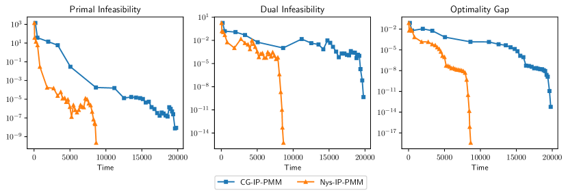
Figure 1: Relative primal/dual infeasibility and optimality gap versus cumulative time for portfolio optimization problem with $n=$80\,000$$, $d=$50\,000$$, and $s=100$. Chol-IP-PMM does not complete any single iteration within $20\,000$ seconds.

5.2 Support vector machine (SVM) problem

The linear support vector machine (SVM) problem solves a binary classification task on $n$ samples with $d$ features [12, Chap. 12]. It is well-known that dual linear SVM with $\ell_{1}$-regularization can be formulated as a convex QP [14, 59, 23, 58]. See the formulation we used in section C.2. In this example, the constraint matrix $A$ contains the feature matrix as a block and thus can be very dense. We use the medium-to-large sized real datasets from UCI [29] and LIBSVM [8] listed in Table 3.

Table 3: SVM Datasets information.

Datasets	Features $d$	Instances $n$	nnz %	Datasets	Features $d$	Instances $n$	nnz %
SensIT	$100$	$98\,528$	100.0	Arcene	$10\,000$	100	54.1
CIFAR10	$3072$	$60\,000$	99.7	Dexter	$20\,000$	300	0.5
STL-10	$27\,648$	$13\,000$	96.3	Sector	$55\,197$	$9619$	0.3
RNASeq	$20\,531$	$801$	85.8

5.2.1 SVM results

Table 4: Nys-IP-PMM vs other preconditioners on SVM problem.

Datasets	Nys-IP-PMM			CG-IP-PMM			Chol-IP-PMM
	IP-PMM Outer Iter.	Sum of Inner Iter.	Time (sec.)	IP-PMM Outer Iter.	Sum of Inner Iter.	Time (sec.)	IP-PMM Outer Iter.	Sum of Inner Iter.	Time (sec.)
CIFAR10	12	$18\,988$	698.959	$\ast$	$\ast$	$\ast$	$\ast$	$\ast$	$\ast$
RNASeq	14	$4810$	30.2827	14	$25\,080$	93.3229	14	$20\,685$	1484.8
STL-10	21	$35\,886$	6708.41	22	$375\,057$	$30\,075.5$	21	$393\,868$	$2.025\,12\text{\times}{10}^{5}$
SensIT	15	1616	5.38175	15	4483	10.6173	15	1164	7.05179
Arcene	5	388	0.19737	5	648	0.128865	5	6105	44.3508
Dexter	4	338	0.152985	4	332	0.122333	4	3891	51.6747
Sector	16	$3498$	23.5251	16	$4513$	25.4651	16	6925	$2635.24$

This section evaluates the performance of Nys-IP-PMM on the SVM problem (62) using datasets listed in Table 3. We solve SVM problems with Nys-IP-PMM, CG-IP-PMM, and Chol-IP-PMM. All three methods are matrix-free, meaning they do not rely on direct access to the entries of $N_{k}+\delta_{k}I$. The results, presented in Table 4, highlight the effectiveness Nys-IP-PMM. In contrast, Chol-IP-PMM does not improve runtime as much, and in some cases, can even increase the required number of inner iterations (e.g., for Arcene, Dexter, and Sector). Its construction time can also be significant. Overall, Chol-IP-PMM is often much slower than CG-IP-PMM.

The randomized Nyström preconditioner accelerates IP-PMM more effectively on dense datasets such as SensIT, CIFAR10, STL-10, and RNASeq. As indicated in Table 2, the construction time of the Nyström preconditioner differs significantly from that of the partial Cholesky preconditioner when $A$ is dense. Datasets Arcene and Dexter are relatively easy, requiring few inner iterations even without a preconditioner.

In summary, the randomized Nyström preconditioner is a competitive choice for SVM problems. It effectively preconditions ill-conditioned instances without much slowdown for well-conditioned instances.

5.2.2 Condition numbers at different IP-PMM stages

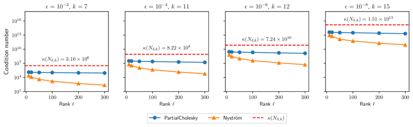
Figure 2: The condition numbers before and after preconditioning. The subplots represent distinct stages of IP-PMM convergence. The red dashed line shows the unpreconditioned condition number $\kappa(N_{\delta,k})$. Blue circles denote the condition number after partial Cholesky preconditioning, while orange triangles represent the condition number after Nyström preconditioning.

We explore the impact of the preconditioner across various stages of IP-PMM by examining the condition number. We record the regularized normal equations (6) in the iteration of which IP-PMM attains primal-dual infeasibility and duality measure less than different tolerance levels $\epsilon\in\{10^{-2},10^{-4},10^{-6},10^{-8}\}$. Then we compute the condition number of $N_{\delta}=N_{k}+\delta_{k}I$ before and after applying different preconditioners. For efficiency, this experiment concerns a smaller SVM problem formed from $1000$ samples from CIFAR10; the normal equations have size $3073\times 3073$.

Figure 2 demonstrates the (preconditioned) condition numbers with different choices $\ell\in\{10,20,50,100,200,300\}$. The red dashed horizontal line denotes the condition number $\kappa(N_{\delta})$ before preconditioning. The blue circles denote the condition numbers after partial Cholesky preconditioning, while the orange triangles denote those after Nyström preconditioning. As expected, the normal equation matrix $N_{\delta}$ becomes more and more ill-conditioned as IP-PMM converges. The preconditioners have similar effects at each stage of convergence. Both preconditioners reduce the condition number by 1–2 orders of magnitude. As the rank $\ell$ increases, the Nyström preconditioner improves the condition number by another 1–2 orders of magnitude, while larger ranks barely improve the effectiveness of partial Cholesky preconditioner.

5.2.3 Rank $\ell$ versus total/construction/PCG Time

We illustrate trade-offs between the rank $\ell$ and the wallclock time of Nys-IP-PMM and Chol-IP-PMM. Figure 3 shows the wallclock time for SVM problem on the RNASeq dataset, where the normal equations have dimension $$20\,532$\times$20\,532$$.

The left subplot of Figure 3 shows that the Nyström preconditioner reduces overall runtime dramatically compared to the partial Cholesky preconditioner. PCG runtime for the partial Cholesky preconditioner barely decreases and later even increases with increased rank. This phenomenon shows a limitation in the effectiveness of the partial Cholesky preconditioner. Fluctuation in the construction time for partial Cholesky preconditioner may be due to the computation of $\operatorname{diag}(S)$. This operation involves $m-\ell$ matrix-vector products with $N_{\delta,21}N_{\delta,11}^{-1}N_{\delta,21}^{T}$, and the size of $N_{\delta,21}$ ($(m-\ell)\times\ell$) does not monotonically increase with $\ell$.

Zooming in, the right subplot of Figure 3 shows the trade-off between the rank parameter $\ell$ and the total time for Nys-IP-PMM. The PCG runtime dominates for smaller ranks, while the time to construct the preconditioner dominates for higher ranks. The overall time exhibits a U-shape: excessively small or large ranks lead to slower computational times. Improvements to Nys-IP-PMM might be achieved by tuning the rank for each problem and by reusing the preconditioner between iterations.

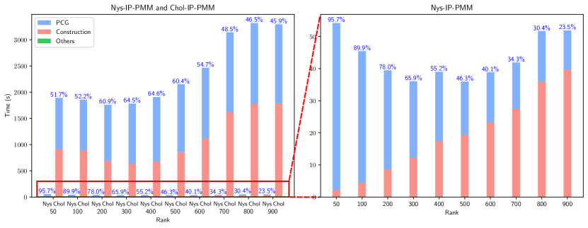
Figure 3: Runtime of Nys-IP-PMM and Chol-IP-PMM with varying rank $\ell$ on RNASeq dataset. Left plot compares the two methods; right plot zooms in on the bar chart for Nys-IP-PMM. Bar height show total runtime, which is broken into 1) PCG runtime, 2) construction time for preconditioner, and 3) other computation (which is negligible). Blue number above bar gives percentage PCG time.

6 Concluding remarks

We present a new algorithm, Nys-IP-PMM, for large-scale separable QP by solving subproblems of IP-PMM using randomized Nyström preconditioned conjugate gradient. Nys-IP-PMM leverages matrix-free preconditioning for computational efficiency. Theoretical analysis and numerical experiments demonstrate superiority of Nys-IP-PMM over existing matrix-free IPM-based methods. By combining theoretical insights with empirical validation, our work advances the state-of-the-art in large-scale optimization, with potential applications in finance, engineering, and machine learning.

Appendix A Proofs

A.1 Lemmas for Theorem 3.1

This section provides the lemmas supporting Theorem 3.1, which is built upon [48, Lemma 1–4], Lemma A.1 and Lemma A.2. Note that [48, Lemma 1–4] were originally devised for exact IP-PMM, yet their proofs still hold for inexact IP-PMM, provided that the iterates $(x^{k},y^{k},z^{k})$ lie within the neighborhood $\mathcal{N}_{\mu_{k}}\left(\zeta^{k},\lambda^{k}\right)$ defined in (18). This condition is established in Lemmas A.1 and A.2, adapted from [48, Lemma 5–6] respectively. The modifications are inspired by the techniques used for inexact IP-PMM on linearly constrained SDP [49].

Lemma A.1.

Assume Assumptions 3.2 and 3.3 and suppose that the search direction $\left(\Delta x^{k},\Delta y^{k},\Delta z^{k}\right)$ satisfies inexact Newton system (19) at an arbitrary iteration $k\geq 0$ of inexact IP-PMM. Let $D_{k}^{2}:=\operatorname{diag}(x^{k})\operatorname{diag}(z^{k})^{-1}$. Then

$$\left\|D_{k}^{-1}\Delta x^{k}\right\|_{2}=O(n^{2}\mu_{k}^{\frac{1}{2}}),\leavevmode\nobreak\ \left\|D_{k}\Delta z^{k}\right\|_{2}=O(n^{2}\mu_{k}^{\frac{1}{2}}),\leavevmode\nobreak\ \left\|\left(\Delta x^{k},\Delta y^{k},\Delta z^{k}\right)\right\|_{2}=O(n^{3}).$$

Proof.

The proof follows that of [48, Lemma 5] with a few modifications. For simplicity, we only sketch the proof with emphasis on modifications.

Following the beginning of the proof for [48, Lemma 5], we invoke [48, Lemma 2] and [48, Lemma 3] to obtain two triples $(x_{r^{k}}^{\ast},y_{r^{k}}^{\ast},z_{r^{k}}^{\ast})$ and $(\tilde{x},\tilde{y},\tilde{z})$ satisfying [48, Eq. (22)] and [48, Eq. (23)] respectively. Using the centering parameter $\sigma_{k}$, instead of defining $\hat{c}$ and $\hat{b}$ as in [48, Eq. (29)], we define

$$\hat{c} :=-\left(\sigma_{k}\frac{\bar{c}}{\mu_{0}}-\left(1-\sigma_{k}\right)\left(x^{k}-\zeta^{k}+\frac{\mu_{k}}{\mu_{0}}\left(\tilde{x}-x_{r^{k}}^{*}\right)\right)+\frac{1}{\mu_{k}}\varrho_{d}^{k}\right),$$ (34)

$$\hat{b} :=-\left(\sigma_{k}\frac{\bar{b}}{\mu_{0}}+\left(1-\sigma_{k}\right)\left(y^{k}-\lambda^{k}+\frac{\mu_{k}}{\mu_{0}}\left(\tilde{y}-y_{r^{k}}^{*}\right)\right)+\frac{1}{\mu_{k}}\varrho_{p}^{k}\right),$$ (35)

where $\bar{c},\bar{b},\mu_{0}$ are defined in (16). The additional terms $\varrho_{d}^{k}/\mu_{k}$ and $\varrho_{p}^{k}/\mu_{k}$ in (34)–(35) take into account the inexact errors in Newton system (19). With this new pair $(\hat{b},\hat{c})$, define the triple $(\bar{x},\bar{y},\bar{z})$ as in [48, Eq. (31)]. Using [48, Eq. (22)–(23), (31)] and inexact Newton system (19), it can be directly verified that

$$A\bar{x}+\mu_{k}\bar{y}=0,\quad-Q\bar{x}+A^{T}\bar{y}+\bar{z}-\mu_{k}\bar{x}=0.$$ (36)

Additional error terms are absorbed into the inexactness of the Newton system (19), yielding (36). Given (36), the rest of the proof follows the proof of [48, Lemma 5]. ∎

Lemma A.2 serves as the keystone for Theorem 3.1, establishing a connection between inexact and exact IP-PMM. The lemma demonstrates that a step in the inexact search direction with a sufficiently small stepsize yields sufficient reduction in the duality measure (Lemma A.2 (i)) while staying within neighborhood $\mathcal{N}_{\mu_{k}}\left(\zeta^{k},\lambda^{k}\right)$ (Lemma A.2 (iii)). Additionally, it ensures that the stepsizes are uniformly bounded away from zero (for every iteration), on the order of $O(\frac{1}{n^{4}})$ (Lemma A.2 (ii)).

Lemma A.2.

Instate Assumptions 3.2 and 3.3 and assume that the search direction $(\Delta x^{k},\Delta y^{k},\Delta z^{k})$ satisfies the inexact Newton system (19), with inexact errors satisfying Assumption 3.1 for every iteration $k\geq 0$ of inexact IP-PMM. Then there exists a step-length $\bar{\alpha}\in(0,1)$ such that the following hold for all iterations $k\geq 0$:

1. for all $\alpha\in[0,\bar{\alpha}]$,

   $$\left(x^{k}+\alpha\Delta x^{k}\right)^{T}\left(z^{k}+\alpha\Delta z^{k}\right)\geq\left(1-\alpha\left(1-\frac{\sigma_{\min}}{2}\right)\right)(x^{k})^{T}z^{k};$$ (37)

   $$\left(x^{k}_{i}+\alpha\Delta x^{k}_{i}\right)\left(z^{k}_{i}+\alpha\Delta z^{k}_{i}\right)\geq\frac{\gamma_{\mu}}{n}\left(x^{k}+\alpha\Delta x^{k}\right)^{T}\left(z^{k}+\alpha\Delta z^{k}\right),\leavevmode\nobreak\ \forall i\in[n];$$ (38)

   $$\left(x^{k}+\alpha\Delta x^{k}\right)^{T}\left(z^{k}+\alpha\Delta z^{k}\right)\leq\left(1-0.01\alpha\right)(x^{k})^{T}z^{k};$$ (39)

2. $\bar{\alpha}\geq\bar{\kappa}/n^{4}$ with $\bar{\kappa}>0$ being a constant independent of $n$ and $m$;

3. suppose $\left(x^{k},y^{k},z^{k}\right)\in\mathcal{N}_{\mu_{k}}\left(\zeta^{k},\lambda^{k}\right)$ and, for any $\alpha\in(0,\bar{\alpha}]$, let

   $$\left(x^{k+1},y^{k+1},z^{k+1}\right)=\left(x^{k}+\alpha\Delta x^{k},y^{k}+\alpha\Delta y^{k},z^{k}+\alpha\Delta z^{k}\right)$$ (40)

   and $\mu_{k+1}=(x^{k+1})^{T}z^{k+1}/n$. Then

   $$\left(x^{k+1},y^{k+1},z^{k+1}\right)\in\mathcal{N}_{\mu_{k+1}}\left(\zeta^{k+1},\lambda^{k+1}\right),$$ (41)

   where $\lambda^{k}$ and $\zeta^{k}$ are updated as in Algorithm 2.

Proof.

The proof follows that of [48, Lemma 6]. Again, we only sketch the outline of the proof and point out the necessary modifications. The assumption $\varrho_{\mu}^{k}=0$ in Assumption 3.1 guarantees the third block of Newton system (19) is exact, so the same argument in the proof of [48, Lemma 6] can show that (37)–(39) holds for every $\alpha\in(0,\alpha^{\ast})$ with exactly the same $\alpha^{\ast}$ in [48, Eq. (40)], i.e.,

$$\alpha^{*}\coloneqq\min\left\{\frac{\sigma_{\min}}{2C_{\Delta}^{2}n^{3}},\frac{\sigma_{\min}\left(1-\gamma_{\mu}\right)}{2C_{\Delta}^{2}n^{4}},\frac{0.49}{C_{\Delta}^{2}n^{3}},1\right\},$$ (42)

where $C_{\Delta}>0$ is a constant such that $(\Delta x^{k})^{T}\Delta z^{k}\leq\|D_{k}^{-1}\Delta x^{k}\|_{2}\|D_{k}\Delta z^{k}\|_{2}\leq C_{\Delta}^{2}n^{4}\mu_{k}$ from Lemma A.1. Next, we must find the maximal $\bar{\alpha}\in(0,\alpha^{\ast}]$ such that

$$\left(x^{k}(\alpha),y^{k}(\alpha),z^{k}(\alpha)\right)\in\mathcal{N}_{\mu_{k}(\alpha)}(\zeta^{k},\lambda^{k}),\quad\text{for all }\alpha\in(0,\bar{\alpha}],$$ (43)

where $\mu_{k}(\alpha)=\frac{x(\alpha)^{T}z(\alpha)}{n}$ and

$$\left(x^{k}(\alpha),y^{k}(\alpha),z^{k}(\alpha)\right)=\left(x^{k}+\alpha\Delta x^{k},y^{k}+\alpha\Delta y^{k},z^{k}+\alpha\Delta z^{k}\right).$$

By definitions (17) and (18), eq. 43 is equivalent to

$$\left\|\tilde{r}_{p}(\alpha),\tilde{r}_{d}(\alpha)\right\|_{2}\leq C_{N}\tfrac{\mu_{k}(\alpha)}{\mu_{0}},\quad\left\|\tilde{r}_{p}(\alpha),\tilde{r}_{d}(\alpha)\right\|_{\mathcal{A}}\leq\gamma_{\mathcal{A}}\rho\tfrac{\mu_{k}(\alpha)}{\mu_{0}},\quad\forall\alpha\in(0,\bar{\alpha}],$$ (44)

where $\tilde{r}_{p}(\alpha)$ and $\tilde{r}_{d}(\alpha)$ are the residuals of two equalities in $\tilde{\mathcal{C}}_{\mu_{k}}\left(\zeta^{k},\lambda^{k}\right)$ in (17):

$$\tilde{r}_{p}(\alpha) =Ax^{k}(\alpha)+\mu_{k}(\alpha)\left(y^{k}(\alpha)-\lambda^{k}\right)-\left(b+\frac{\mu_{k}(\alpha)}{\mu_{0}}\bar{b}\right),$$

$$\tilde{r}_{d}(\alpha) =-Qx^{k}(\alpha)+A^{T}y^{k}(\alpha)+z^{k}(\alpha)-\mu_{k}(\alpha)\left(x^{k}(\alpha)-\zeta^{k}\right)-\left(c+\frac{\mu_{k}(\alpha)}{\mu_{0}}\bar{c}\right).$$

Following the calculations in the proof of [48, Lemma 6], now with the inexact Newton system (19), the two residuals $\tilde{r}_{p}(\alpha)$ and $\tilde{r}_{d}(\alpha)$ have additional inexact error terms $\alpha\varrho_{p}^{k}$ and $\alpha\varrho_{d}^{k}$ respectively:

$$\tilde{r}_{p}(\alpha) =(1-\alpha)\frac{\mu_{k}}{\mu_{0}}\tilde{b}^{k}+\alpha^{2}\left(\sigma_{k}-1\right)\mu_{k}\Delta y^{k}+\alpha^{2}\tfrac{(\Delta x^{k})^{T}\Delta z^{k}}{n}\left(y^{k}-\lambda^{k}+\alpha\Delta y^{k}-\frac{\bar{b}}{\mu_{0}}\right)+\alpha\varrho_{p}^{k},$$

$$\tilde{r}_{d}(\alpha) =(1-\alpha)\frac{\mu_{k}}{\mu_{0}}\tilde{c}^{k}-\alpha^{2}\left(\sigma_{k}-1\right)\mu_{k}\Delta x^{k}-\alpha^{2}\tfrac{(\Delta x^{k})^{T}\Delta z^{k}}{n}\left(x^{k}-\zeta^{k}+\alpha\Delta x^{k}+\frac{\bar{c}}{\mu_{0}}\right)+\alpha\varrho_{d}^{k}.$$

Using the same quantities $\xi_{2}=O(n^{4}\mu_{k})$ and $\xi_{\mathcal{A}}=O(n^{4}\mu_{k})$ defined as in [48, Eq. (44)], we have the bounds

$$\left\|(\tilde{r}_{p}(\alpha),\tilde{r}_{d}(\alpha))\right\|_{2} \leq(1-\alpha)C_{N}\frac{\mu_{k}}{\mu_{0}}+\alpha^{2}\mu_{k}\xi_{2}+\alpha\|(\varrho_{p}^{k},\varrho_{d}^{k})\|_{2},$$

$$\left\|(\tilde{r}_{p}(\alpha),\tilde{r}_{d}(\alpha))\right\|_{\mathcal{A}} \leq(1-\alpha)\gamma_{\mathcal{A}}\rho\frac{\mu_{k}}{\mu_{0}}+\alpha^{2}\mu_{k}\xi_{\mathcal{A}}+\alpha\|(\varrho_{p}^{k},\varrho_{d}^{k})\|_{\mathcal{A}},$$

for all $\alpha\in(0,\alpha^{\ast}]$, where $\alpha^{\ast}$ is given by (42). Assumption Assumption 3.1 on error bounds for the inexactness further yields that, for all $\alpha\in(0,\alpha^{\ast}]$,

$$\left\|\tilde{r}_{p}(\alpha),\tilde{r}_{d}(\alpha)\right\|_{2} \leq\frac{C_{N}}{\mu_{0}}\left(1-\alpha\left(1-\frac{\sigma_{\min}}{4}-\alpha\frac{\mu_{0}\xi_{2}}{C_{N}}\right)\right)\mu_{k},$$ (45)

$$\left\|\tilde{r}_{p}(\alpha),\tilde{r}_{d}(\alpha)\right\|_{\mathcal{A}} \leq\frac{\gamma_{\mathcal{A}}\rho}{\mu_{0}}\left(1-\alpha\left(1-\frac{\sigma_{\min}}{4}-\alpha\frac{\mu_{0}\xi_{\mathcal{A}}}{\gamma_{\mathcal{A}}\rho}\right)\right)\mu_{k}.$$ (46)

On the other hand, (37) implies $\mu_{k}(\alpha)\geq\left(1-\alpha\left(1-\frac{\sigma_{\min}}{2}\right)\right)\mu_{k}$ for all $\alpha\in(0,\alpha^{\ast}]$, which together with (45)–(46) yields

$$\left\|\tilde{r}_{p}(\alpha),\tilde{r}_{d}(\alpha)\right\|_{2} \leq\frac{\mu_{k}(\alpha)}{\mu_{0}}C_{N},\quad \text{for all }\alpha\in\left(0,\min\left\{\alpha^{*},\frac{\sigma_{\min}C_{N}}{4\xi_{2}\mu_{0}}\right\}\right];$$

$$\left\|\tilde{r}_{p}(\alpha),\tilde{r}_{d}(\alpha)\right\|_{\mathcal{A}} \leq\frac{\mu_{k}(\alpha)}{\mu_{0}}\gamma_{\mathcal{A}}\rho,\quad \text{for all }\alpha\in\left(0,\min\left\{\alpha^{*},\frac{\sigma_{\min}\gamma_{\mathcal{A}}\rho}{4\xi_{\mathcal{A}}\mu_{0}}\right\}\right].$$

Finally, let

$$\bar{\alpha}^{k}\coloneqq\min\left\{\alpha^{*},\frac{\sigma_{\min}C_{N}}{4\xi_{2}\mu_{0}},\frac{\sigma_{\min}\gamma_{\mathcal{A}}\rho}{4\xi_{\mathcal{A}}\mu_{0}}\right\}\leavevmode\nobreak\ \text{ and }\leavevmode\nobreak\ \bar{\alpha}\coloneqq\min_{k\geq 0}\bar{\alpha}^{k}.$$ (47)

Since $\xi_{2}=O(n^{4}\mu_{k})$, $\xi_{\mathcal{A}}=O(n^{4}\mu_{k})$, and $\mu_{k}$ is decreasing, there must exist a constant $\bar{\kappa}>0$, independent of $n,m$, and $k$ such that $\bar{\alpha}^{k}\geq\frac{\bar{\kappa}}{n^{4}}$ for all $k\geq 0$, and hence $\bar{\alpha}\geq\frac{\bar{\kappa}}{n^{4}}$. This proves (i) and (ii). To prove (iii), we divide into two cases:

• Suppose the estimates $\zeta^{k}$ and $\lambda^{k}$ are not updated, that is, $\zeta^{k+1}=\zeta^{k}$ and $\lambda^{k+1}=\lambda^{k}$. The choice of $\bar{\alpha}$ in (47) guarantees (44) and hence (43), so that the new iterate in (40) satisfies (41).

• Suppose IP-PMM updates the estimates $\zeta^{k}$ and $\lambda^{k}$, that is, $\zeta^{k+1}=x^{k+1}$ and $\lambda^{k+1}=y^{k+1}$. This happens only when

  $$\left\|(r_{p},r_{d})\right\|_{2}\leq C_{N}\frac{\mu_{k+1}}{\mu_{0}},\quad\left\|(r_{p},r_{d})\right\|_{\mathcal{A}}\leq\gamma_{\mathcal{A}}\rho\frac{\mu_{k+1}}{\mu_{0}},$$ (48)

  where $r_{p}=Ax^{k+1}-(b+\frac{\mu_{k+1}}{\mu_{0}}\bar{b})$ and $r_{d}=(c+\frac{\mu_{k+1}}{\mu_{0}}\bar{c})+Qx^{k+1}-A^{T}y^{k+1}-z^{k+1}$. Condition (48) is exactly equivalent to (41).

∎

A.2 Proof of Proposition 3.1

Proof.

We omit the proof for $(\varrho_{d}^{k},\varrho_{p}^{k},\varrho_{\mu}^{k})=(0,\vartheta^{k},0)$ as it follows from direct calculations. The equality and bounds for $2$-norm in (21) follows directly from the fact $(\varrho_{d}^{k},\varrho_{p}^{k},\varrho_{\mu}^{k})=(0,\vartheta^{k},0)$ and the assumption $\|\vartheta^{k}\|_{2}\leq C\mu_{k}$. To verify bound for semi-norm $\|(\varrho_{p}^{k},\varrho_{d}^{k})\|_{\mathcal{A}}$, observe that

$$\|(\varrho_{p}^{k},\varrho_{d}^{k})\|_{\mathcal{A}}=\|(0,\epsilon)\|_{\mathcal{\mathcal{A}}}=\min_{x,y,z}\left\{\|(x,z)\|_{2}\mid Ax=0,\leavevmode\nobreak\ -Qx+A^{T}y+z=\epsilon\right\},$$

and $(\tilde{x},\tilde{y},\tilde{z})=(0,0,\vartheta^{k})$ is a solution to the systems $Ax=0$ and $-Qx+A^{T}y+z=\vartheta^{k}$, so that $\|(\varrho_{p}^{k},\varrho_{d}^{k})\|_{\mathcal{\mathcal{A}}}\leq\left\|\left(\tilde{x},\tilde{z}\right)\right\|_{2}=\|(0,\vartheta^{k})\|_{2}\leq C\mu_{k}$. ∎

A.3 Proof of Theorem 4.1 and required lemmas

This section presents the proof of Theorem 4.1 and the necessary lemmas. Lemma A.3 from [61] gives the number of Nyström PCG iterations to obtain a solution within error $\varepsilon$.

Lemma A.3 ([61, Corollary 4.2]).

Let $\delta>0$ and consider regularized system

$$(N+\delta I)\Delta y=\xi.$$ (49)

Suppose $P$ is the Nyström preconditioner constructed as in (13) and sketch size $\ell\geq 8\left(\sqrt{d_{\text{eff}}(\delta)}+\sqrt{8\log(16/\eta)}\right)^{2}.$ Let $\Delta y^{\ast}$ denote the true solution of (49) and $\{\Delta y^{(t)}\}_{t\geq 1}$ denote the iterates generated by Nyström PCG on problem (49). Then with probability at least $1-\eta$, it holds true that $\|\Delta y^{(t)}-\Delta y^{\star}\|_{2}\leq\varepsilon$ after $t=O(\log(\|\Delta y^{\star}\|_{2}/\varepsilon))$ iterations.

Based on Lemma A.3, we present next Lemma A.4 showing that at each iteration $k$ of Nys-IP-PMM, Nyström PCG can return a solution with small inexact error after a few iterations, when the Newton system (19) is solved by the normal equations. For simplicity of presentation, we drop the iteration superindex $k$ in the statement and proof of the lemma.

Lemma A.4.

Let $N=A(Q+\Theta^{-1}+\mu I_{n})^{-1}A^{T}$. Given Assumptions 3.2 and 3.3, suppose the regularized normal equations (20) is solved by PCG using the randomized Nyström preconditioner (13) with $\delta=\mu$ and sketch size

$$\ell\geq 8\left(\sqrt{d_{\text{eff}}(\mu)}+\sqrt{8\log(16/\eta)}\right)^{2},$$ (50)

where $d_{\text{eff}}(\cdot)$ is the effective dimension of $N$ defined in (15). Let $\{\Delta y^{(t)}\}_{t\geq 1}$ denote the iterates generated by Nyström PCG. Then, with probability at least $1-\eta$, after $t=O\left(\log(\frac{n}{\varepsilon\mu})\right)$ iterations, the residual satisfies

$$\left\|(N+\mu I)\Delta y^{(t)}-\xi\right\|_{2}\leq\varepsilon.$$ (51)

Proof.

We abbreviate the regularized matrix as $N_{\mu}=N+\mu I$ and let $\Delta y^{\star}$ denote the true solution of (6) (with $\rho=\delta=\mu$). Let $r^{(t)}=N_{\mu}\Delta y^{(t)}-\xi$ denote the residual at $t$-th iteration. It follows from norm consistency and $\|N_{\mu}\|_{2}=\lambda_{\max}(N_{\mu})$ that $\|r^{(t)}\|_{2}\leq\lambda_{\max}(N_{\mu})\|\Delta y^{(t)}-\Delta y^{\star}\|_{2}$. Hence, we would have $\|r^{(t)}\|_{2}\leq\varepsilon$ if

$$\|\Delta y^{(t)}-\Delta y^{\star}\|_{2}\leq\varepsilon/\lambda_{\max}(N_{\mu}).$$ (52)

By Lemma A.3, with probability at least $1-\eta$, inequality (52) holds true after

$$t=O\left(\log\left(\frac{\lambda_{\max}(N_{\mu})\|\Delta y^{\star}\|_{2}}{\varepsilon}\right)\right)$$ (53)

PCG iterations. Assumption 3.3 and Lemma A.1 respectively guarantee that

$$\lambda_{\max}(N_{\mu})=\left\|A(Q+\Theta+\mu I)^{-1}A^{T}\right\|_{2}+\mu=O\left(\frac{1}{\mu}\right)\text{ and }\left\|\Delta y^{\star}\right\|_{2}=O\left(n^{3}\right).$$

Therefore, the required number of iterations (53) becomes $t=O\left(\log(\frac{n}{\varepsilon\mu})\right).$ ∎

Proof of Theorem 4.1.

To guarantee the convergence, the inexact errors of IP-PMM have to satisfy Assumption 3.1, which holds true if, by Proposition 3.1, the inexact error $\vartheta^{k}$ in (20) satisfies

$$\|\vartheta^{k}\|_{2}\leq\frac{\sigma_{\min}}{4\mu_{0}}\min\left\{C_{N},\gamma_{\mathcal{A}}\rho\right\}\mu_{k}.$$ (54)

At each iteration $k$ of Nys-IP-PMM, we take the sketch size $\ell_{k}$ as in (23) and $\eta_{k}\coloneqq\frac{1}{(k+2)^{4}}$ for all $k\geq 0$, so that (50) in Lemma A.4 is satisfied, which guarantees, with probability at least $1-\eta_{k}$, that Nyström PCG satisfies (54) with order of iterations given by $O(\log\frac{n}{C\mu_{k}^{2}})=O(\log(n/\varepsilon))$, where $C\coloneqq\frac{\sigma_{\min}}{4\mu_{0}}\min\left\{C_{N},\gamma_{\mathcal{A}}\rho\right\}$. To get this, we use the fact that $\frac{1}{\mu_{k}}=O(\frac{1}{\varepsilon})$ before Nys-IP-PMM terminates. By intersecting all these events across iteration count $k$, we conclude: with probability at least $1-\sum_{k=0}^{\infty}\frac{1}{(k+2)^{4}}\approx 0.91$. Nyström PCG terminates within $t=O(\log\frac{n}{\varepsilon})$ steps and the residual error of PCG satisfies (54) for all $k\geq 0$, which proves (i).

Proposition 3.1 then guarantees that $(\Delta x^{k},\Delta y^{k},\Delta z^{k})$ satisfies inexact Newton system (19) with inexact errors satisfying Assumption 3.1. Now, we are under the assumptions of Theorem 3.1, so we have $\mu_{k}\leq\varepsilon$ after $k=O(n^{4}\log\frac{1}{\varepsilon})$ iterations of Nys-IP-PMM, as required in (ii). ∎

Appendix B Details on implementation of Nys-IP-PMM

Nys-IP-PMM deviates from the theory in order to improve the computational efficiency, following [48] in the following two main aspects: First, we do not limit to $\rho_{k}=\delta_{k}=\mu_{k}$ as theory does. The proximal parameters $\rho_{k}$ and $\delta_{k}$ are independently updated following the suggestions from [48, Algorithm PEU]. Second, the iterates of the method are not required to lie in the neighborhood as in (18) for efficiency.

The followings provide more details/explanations for the implementation of Nys-IP-PMM. Section B.1 derives the Newton system to be solved at each Nys-IP-PMM iteration for QP instance taking the form $(\tilde{\text{P}})$–$(\tilde{\text{D}})$ and the resulting normal equations. Section B.2 details the construction of practical initial point.

B.1 Derivations of Newton system and equations (25)–(29)

Given QP in the form $(\tilde{\text{P}})$–$(\tilde{\text{D}})$, IP-PMM solves a sequence of subproblems taking the form (24). Introducing the logarithmic barrier function to enforce the constraints $x^{\mathcal{I}}\geq 0$ and $0\leq x^{\mathcal{J}}\leq u^{\mathcal{J}}$ in (24), the Lagrangian to minimize becomes

$$\mathcal{L}(x)=\frac{1}{2}x^{T}Qx+c^{T}x+(\lambda^{k})^{T}(b-Ax) +\frac{1}{2\delta_{k}}\|Ax-b\|_{2}^{2}+\frac{\rho_{k}}{2}\|x-\zeta^{k}\|^{2}$$

$$-\mu_{k}\sum_{j\in\mathcal{I}\mathcal{J}}\ln x_{j}-\mu_{k}\sum_{j\in\mathcal{J}}\ln(u_{j}-x_{j}).$$

Setting $\nabla_{x}\mathcal{L}(x)=0$ and introducing the new variables

$$y=\lambda^{k}-\frac{1}{\mu_{k}}(Ax-b),\quad z_{j}=\begin{cases}\mu_{k}x_{j}^{-1},&\text{if }j\in\mathcal{I}\mathcal{J};\\ 0,&\text{if }j\in\mathcal{F},\end{cases}$$

$$w_{j}=\begin{cases}u_{j}-x_{j},&\text{if }j\in\mathcal{J};\\ 0,&\text{if }j\in\mathcal{I}\mathcal{F},\end{cases}\quad s_{j}=\begin{cases}\mu_{k}w_{j}^{-1},&\text{if }j\in\mathcal{J};\\ 0,&\text{if }j\in\mathcal{I}\mathcal{F},\end{cases}$$

we obtain the following (non-linear) system to solve:

$$\begin{bmatrix}c+Qx-A^{T}y-z+s+\rho_{k}(x-\zeta^{k})\\ Ax-b+\delta_{k}(y-\lambda^{k})\\ x^{\mathcal{J}}+w^{\mathcal{J}}-u^{\mathcal{J}}\\ \operatorname{diag}(x^{\mathcal{I}\mathcal{J}})z^{\mathcal{I}\mathcal{J}}-\mu_{k}\mathbbm{1}_{|\mathcal{I}\mathcal{J}|}\\ \operatorname{diag}(w^{\mathcal{J}})s^{\mathcal{J}}-\mu_{k}\mathbbm{1}_{|\mathcal{J}|}\end{bmatrix}=\begin{bmatrix}0\\ 0\\ 0\\ 0\\ 0\end{bmatrix}.$$ (55)

Applying Newton’s method to (55) yields the Newton system taking the form:

$$\begin{bmatrix}-\left(Q+\rho_{k}I_{n}\right)&A^{T}&0&I_{n}&-I_{n}\\ A&\delta_{k}I_{m}&0&0&0\\ E_{\mathcal{J}}&0&E_{\mathcal{J}}&0&0\\ E_{\mathcal{I}\mathcal{J}}Z_{k}&0&0&E_{\mathcal{I}\mathcal{J}}X_{k}&0\\ 0&0&E_{\mathcal{J}}S_{k}&0&E_{\mathcal{J}}W_{k}\end{bmatrix}\begin{bmatrix}\Delta x^{k}\\ \Delta y^{k}\\ \Delta w^{k}\\ \Delta z^{k}\\ \Delta s^{k}\end{bmatrix}=\begin{bmatrix}r_{d}\\ r_{p}\\ (r_{u})_{\mathcal{J}}\\ (r_{xz})_{\mathcal{I}\mathcal{J}}\\ (r_{ws})_{\mathcal{J}}\end{bmatrix}$$ (56)

where $E_{\mathcal{S}}:\mathbb{R}^{n}\rightarrow\mathbb{R}^{|\mathcal{S}|}$ is the projection matrix such that $E_{\mathcal{S}}x=x^{\mathcal{S}}$ for all $x\in\mathbb{R}^{n}$, the uppercase letters $X^{k},Z^{k},W^{k},S^{k}$ represent diagonal matrices with diagonal entries corresponding to the iterates in the associated lowercase letters, and $r_{d},r_{p},r_{u},r_{xz},r_{ws}$ are appropriate RHS vectors. By eliminating the variables $\Delta x^{k},\Delta w^{k},\Delta z^{k},$ and $\Delta s^{k}$, the Newton system (56) simplifies to the normal equations (25) of size $m$, and four closed-form formulae (26)–(29).

B.2 Construction for initial point

The construction is based on the development of initial point for original IP-PMM in [48]. We first construct a candidate point by ignoring the non-negative constraints and solving the primal and dual equality constraints $Ax=b$ and $-Qx+A^{T}y+z-s=c$ in $(\tilde{\text{P}})$–$(\tilde{\text{D}})$. We force primal candidate $\tilde{x}$ satisfy $Ax=b$ while centering around $u/2$, and solve the dual candidate $\tilde{y}$ from the least squares problem $\min_{y}\|-Q\tilde{x}+A^{T}y-c\|_{2}$, ignoring $z$ and $s$ in dual constraint meanwhile. Then dual candidates $\tilde{z}$ and $\tilde{s}$ are chosen such that dual constraint $-Q\tilde{x}+A^{T}\tilde{y}+\tilde{z}-\tilde{s}=c$ is satisfied. The primal candidate $\tilde{w}$ is set as $\tilde{w}_{\mathcal{J}}=u_{\mathcal{J}}-\tilde{x}_{\mathcal{J}}$ and $\tilde{w}_{\mathcal{I}\mathcal{F}}=0$. In summary, the candidate point is:

$$\tilde{x}=\frac{u}{2}+A^{T}(AA^{T})^{-1}\left(b-\frac{1}{2}Au\right),\quad\tilde{y}=(AA^{T})^{-1}A(c+Q\tilde{x}),$$

$$\tilde{z}_{\mathcal{J}}=\frac{1}{2}\left(c-A^{T}\tilde{y}+Q\tilde{x}\right)_{\mathcal{J}},\quad\tilde{z}_{\mathcal{I}\mathcal{F}}=\left(c-A^{T}\tilde{y}+Q\tilde{x}\right)_{\mathcal{I}\mathcal{F}},$$

$$\tilde{s}_{\mathcal{J}}=-\tilde{z}_{\mathcal{J}},\quad\tilde{s}_{\mathcal{I}\mathcal{F}}=0,\quad\tilde{w}_{\mathcal{J}}=u_{\mathcal{J}}-\tilde{x}_{\mathcal{J}},\quad\tilde{w}_{\mathcal{I}\mathcal{F}}=0.$$

However, to ensure the stability and efficiency, we regularize the matrix $AA^{T}$ as in [48] and use Nyström PCG to solve for the systems in $\tilde{x}$ and $\tilde{y}$, for which the regularization parameter is taken as $\delta=10$.

Next, to guarantee the positivity of $x_{\mathcal{I}\mathcal{J}}$, $z_{\mathcal{I}\mathcal{J}}$, $w_{\mathcal{J}}$, and $s_{\mathcal{J}}$, we compute the following quantities:

$$\delta_{p}=\max\{-1.5\min(\tilde{x}_{\mathcal{I}\mathcal{J}}),-1.5\min(\tilde{w}_{\mathcal{J}}),0\},$$

$$\delta_{d}=\max\{-1.5\min(\tilde{z}_{\mathcal{I}\mathcal{J}}),-1.5\min(\tilde{s}_{\mathcal{J}}),0\},$$

$$\gamma_{xz}=(\tilde{x}_{\mathcal{I}\mathcal{J}}+\delta_{p}\mathbbm{1}_{|\mathcal{I}\mathcal{J}|})^{T}(\tilde{z}_{\mathcal{I}\mathcal{J}}+\delta_{d}\mathbbm{1}_{|\mathcal{I}\mathcal{J}|}),$$

$$\gamma_{ws}=(\tilde{w}_{\mathcal{J}}+\delta_{p}\mathbbm{1}_{|\mathcal{J}|})^{T}(\tilde{s}_{\mathcal{J}}+\delta_{d}\mathbbm{1}_{|\mathcal{J}|}),$$

$$\tilde{\delta}_{p}=\delta_{p}+0.5\frac{\gamma_{xz}+\gamma_{ws}}{\sum_{\ell\in\mathcal{I}\mathcal{J}}(\tilde{z}^{\ell}+\delta_{d})+\sum_{\ell\in\mathcal{J}}(\tilde{s}^{\ell}+\delta_{d})},$$

$$\tilde{\delta}_{d}=\delta_{d}+0.5\frac{\gamma_{xz}+\gamma_{ws}}{\sum_{\ell\in\mathcal{I}\mathcal{J}}(\tilde{x}^{\ell}+\delta_{d})+\sum_{\ell\in\mathcal{J}}(\tilde{w}^{\ell}+\delta_{d})}.$$

Finally, we set the final initial point as:

$$y^{0}=\tilde{y},\quad x^{0}_{\mathcal{I}\mathcal{J}}=\tilde{x}_{\mathcal{I}\mathcal{J}}+\tilde{\delta}_{p}\mathbbm{1}_{|\mathcal{I}\mathcal{J}|},\quad x^{0}_{\mathcal{F}}=\tilde{x}_{\mathcal{F}},$$ (57)

$$w^{0}_{\mathcal{J}}=\tilde{w}_{\mathcal{J}}+\tilde{\delta}_{p}\mathbbm{1}_{|\mathcal{J}|},\quad w^{0}_{\mathcal{I}\mathcal{F}}=0,$$

$$z^{0}_{\mathcal{I}\mathcal{J}}=\tilde{z}_{\mathcal{I}\mathcal{J}}+\tilde{\delta}_{d}\mathbbm{1}_{|\mathcal{I}\mathcal{J}|},\quad z^{0}_{\mathcal{F}}=0,\quad s^{0}_{\mathcal{J}}=\tilde{s}_{\mathcal{J}}+\tilde{\delta}_{d}\mathbbm{1}_{|\mathcal{J}|},\quad s^{0}_{\mathcal{I}\mathcal{F}}=0.$$

B.3 Stepsizes

The primal and dual stepsizes are chosen as in standard IPMs, which ensure that the updated iterate remains in the non-negative orthant after transitioning from the current iterate $x^{k}$, $z^{k}$, $w^{k}$, and $s^{k}$. Given the search directions $\Delta x^{k}$, $\Delta z^{k}$, $\Delta w^{k}$, and $\Delta s^{k}$, denote the sets of indices for negative components by

$$I_{x} =\{i\in\mathcal{I}\cup\mathcal{J}\mid\Delta x^{k}_{i}<0\};\quad I_{w}=\{i\in\mathcal{J}\mid\Delta w^{k}_{i}<0\};$$

$$I_{z} =\{i\in\mathcal{I}\cup\mathcal{J}\mid\Delta z^{k}_{i}<0\};\quad I_{s}=\{i\in\mathcal{J}\mid\Delta s^{k}_{i}<0\}.$$

The primal and dual stepsizes are defined as follows:

$$\alpha_{p} =0.995\min\left\{1,\min_{i\in I_{x}}\left\{-\frac{x^{k}_{i}}{\Delta x^{k}_{i}}\right\},\min_{i\in I_{w}}\left\{-\frac{w^{k}_{i}}{\Delta w^{k}_{i}}\right\}\right\},$$ (58)

$$\alpha_{d} =0.995\min\left\{1,\min_{i\in I_{z}}\left\{-\frac{z^{k}_{i}}{\Delta z^{k}_{i}}\right\},\min_{i\in I_{s}}\left\{-\frac{s^{k}_{i}}{\Delta s^{k}_{i}}\right\}\right\}.$$ (59)

Appendix C Experimental Details

C.1 QP formulation for portfolio optimization

Consider a portfolio optimization problem, which aims at determining the asset allocation to maximize risk-adjusted returns while constraining correlation with market indexes or competing portfolios:

$$\begin{array}[]{cl}\operatorname{\mathrm{minimize}}&\displaystyle-r^{T}x+\gamma x^{T}\Sigma x\\ \mathrm{subject}\leavevmode\nobreak\ \mathrm{to}&Mx\leq u,\leavevmode\nobreak\ \mathbbm{1}_{n}^{T}x=1,\leavevmode\nobreak\ x\geq 0,\end{array}$$ (60)

where variable $x\in\mathbb{R}^{n}$ represents the portfolio, $r\in\mathbb{R}^{n}$ denotes the vector of expected returns, $\gamma>0$ denotes the risk aversion parameter, $\Sigma\in\mathbb{S}_{n}^{+}(\mathbb{R})$ represents the risk model covariance matrix, each row of $M\in\mathbb{R}^{d\times n}$ represents another portfolio, and $u\in\mathbb{R}^{d}$ upper bounds the correlations.

We assume a factor model for the covariance matrix $\Sigma=FF^{T}+D$, where $F\in\mathbb{R}^{n\times s}$ is the factor loading matrix and $D\in\mathbb{R}^{n\times n}$ is a diagonal matrix representing asset-specific risk. By replacing $\Sigma$ with $FF^{T}+D$ in (60) and introducing a new variable $y=F^{T}x$, we write an equivalent problem in variables $x$ and $y$:

$$\begin{array}[]{cl}\operatorname{\mathrm{minimize}}&\displaystyle-\gamma^{-1}r^{T}x+x^{T}Dx+y^{T}y\\ \mathrm{subject}\leavevmode\nobreak\ \mathrm{to}&y=F^{T}x,\leavevmode\nobreak\ Mx\leq u,\leavevmode\nobreak\ \mathbbm{1}_{n}^{T}x=1,\leavevmode\nobreak\ x\geq 0,\leavevmode\nobreak\ y:\text{free}.\end{array}$$ (61)

Problem (61) can be transformed into form $(\tilde{\text{P}})$ via standard techniques.

C.2 Support vector machine (SVM) formulations in QP

The linear support vector machine (SVM) problem solves a binary classification task on $n$ samples with $d$ features [12, Chapter 12]. Let $X\in\mathbb{R}^{d\times n}$ be a feature matrix whose columns are the attribute vectors $x_{i}\in\mathbb{R}^{d}$ associated with the $i$-th sample, $i=1,\ldots,n$, and let $y_{i}\in\{-1,1\}$ be the corresponding binary classification label. The dual linear SVM with $\ell_{1}$-regularization can be formulated as a convex quadratic program [14, 59, 23, 10, 58]:

$$\begin{array}[]{cl}\operatorname{\mathrm{minimize}}&\displaystyle\frac{1}{2}v^{T}v-\sum_{i=1}^{n}p_{i}\\ \mathrm{subject}\leavevmode\nobreak\ \mathrm{to}&v-X\operatorname{diag}(y)p=0,\leavevmode\nobreak\ y^{T}p=0,\\ &v\text{: free},\leavevmode\nobreak\ 0\leq p_{i}\leq\tau,\leavevmode\nobreak\ i=1,\ldots,n,\end{array}$$ (62)

where $v\in\mathbb{R}^{d}$ and $p\in\mathbb{R}^{n}$ are optimization variables, and $\tau>0$ is the penalty parameter for misclassification. The dual SVM problem (62) can be formulated into form $(\tilde{\text{P}})$ by setting

$$x=\begin{bmatrix}v\\ p\end{bmatrix}\in\mathbb{R}^{d+n},\leavevmode\nobreak\ Q=\begin{bmatrix}I_{d}&\mathbf{0}\\ \mathbf{0}&\mathbf{0}\end{bmatrix}\in\mathbb{R}^{(d+n)\times(d+n)},$$

$$A=\begin{bmatrix}I_{d}&-X\operatorname{diag}(y)\\ \mathbf{0}&y^{T}\end{bmatrix}\in\mathbb{R}^{(d+1)\times(d+n)},\leavevmode\nobreak\ c=\begin{bmatrix}\mathbf{0}_{d}\\ \mathbbm{1}_{n}\end{bmatrix}\in\mathbb{R}^{d+n},\leavevmode\nobreak\ b=\mathbf{0}_{d+1},$$

$$\mathcal{F}=\{1,2,\ldots,d\},\leavevmode\nobreak\ \mathcal{I}=\emptyset,\leavevmode\nobreak\ \mathcal{J}=\{d+1,\ldots,d+n\},\leavevmode\nobreak\ u^{\mathcal{J}}=\tau\mathbbm{1}_{|\mathcal{J}|}.$$

Note that the constraint matrix $A$ has a dense $(1,2)$-block if the feature matrix $X$ is dense.

References

• [1] A. Altman and J. Gondzio, Regularized symmetric indefinite systems in interior point methods for linear and quadratic optimization, Optimization Methods and Software, 11 (1999), pp. 275–302, https://doi.org/10.1080/10556789908805754.
• [2] S. Bellavia, J. Gondzio, and B. Morini, A Matrix-Free Preconditioner for Sparse Symmetric Positive Definite Systems and Least-Squares Problems, SIAM Journal on Scientific Computing, 35 (2013), pp. A192–A211, https://doi.org/10.1137/110840819.
• [3] L. Bergamaschi, J. Gondzio, Á. Martínez, J. W. Pearson, and S. Pougkakiotis, A new preconditioning approach for an interior point-proximal method of multipliers for linear and convex quadratic programming, Numerical Linear Algebra with Applications, 28 (2021), p. e2361, https://doi.org/10.1002/nla.2361.
• [4] J. Bezanson, A. Edelman, S. Karpinski, and V. B. Shah, Julia: A Fresh Approach to Numerical Computing, SIAM Review, 59 (2017), pp. 65–98, https://doi.org/10.1137/141000671.
• [5] S. Bocanegra, F. F. Campos, and A. R. L. Oliveira, Using a hybrid preconditioner for solving large-scale linear systems arising from interior point methods, Computational Optimization and Applications, 36 (2007), pp. 149–164, https://doi.org/10.1007/s10589-006-9009-5.
• [6] L. Casacio, C. Lyra, A. R. L. Oliveira, and C. O. Castro, Improving the preconditioning of linear systems from interior point methods, Computers & Operations Research, 85 (2017), pp. 129–138, https://doi.org/10.1016/j.cor.2017.04.005.
• [7] T. F. Chan, An Optimal Circulant Preconditioner for Toeplitz Systems, SIAM Journal on Scientific and Statistical Computing, 9 (1988), pp. 766–771, https://doi.org/10.1137/0909051.
• [8] C.-C. Chang and C.-J. Lin, LIBSVM: A library for support vector machines, ACM Transactions on Intelligent Systems and Technology, 2 (2011), pp. 1–27, https://doi.org/10.1145/1961189.1961199.
• [9] A. Chowdhury, G. Dexter, P. London, H. Avron, and P. Drineas, Faster randomized interior point methods for Tall/Wide linear programs, Journal of Machine Learning Research, 23 (2022), pp. 1–48, http://jmlr.org/papers/v23/21-0709.html.
• [10] R. Čiegis, D. Henty, B. Kågström, J. Žilinskas, K. Woodsend, and J. Gondzio, High-performance parallel support vector machine training, Parallel Scientific Computing and Optimization: Advances and Applications, (2009), pp. 83–92.
• [11] F. de Prenter, C. V. Verhoosel, G. J. van Zwieten, and E. H. van Brummelen, Condition number analysis and preconditioning of the finite cell method, Computer Methods in Applied Mechanics and Engineering, 316 (2017), pp. 297–327, https://doi.org/10.1016/j.cma.2016.07.006.
• [12] M. P. Deisenroth, A. A. Faisal, and C. S. Ong, Mathematics for machine learning, Cambridge University Press, 2020.
• [13] C. Durazzi and V. Ruggiero, Indefinitely preconditioned conjugate gradient method for large sparse equality and inequality constrained quadratic problems, Numerical Linear Algebra with Applications, 10 (2003), pp. 673–688, https://doi.org/10.1002/nla.308.
• [14] S. Fine and K. Scheinberg, Efficient SVM training using low-rank kernel representations, Journal of Machine Learning Research, 2 (2001), pp. 243–264, https://www.jmlr.org/papers/v2/fine01a.html.
• [15] A. Forsgren, P. E. Gill, and M. H. Wright, Interior Methods for Nonlinear Optimization, SIAM Review, 44 (2002), pp. 525–597, https://doi.org/10.1137/S0036144502414942.
• [16] Z. Frangella, J. A. Tropp, and M. Udell, Randomized Nyström Preconditioning, SIAM Journal on Matrix Analysis and Applications, 44 (2023), pp. 718–752, https://doi.org/10.1137/21M1466244.
• [17] M. P. Friedlander and D. Orban, A primal–dual regularized interior-point method for convex quadratic programs, Mathematical Programming Computation, 4 (2012), pp. 71–107, https://doi.org/10.1007/s12532-012-0035-2.
• [18] P. E. Gill, W. Murray, M. A. Saunders, J. A. Tomlin, and M. H. Wright, On projected newton barrier methods for linear programming and an equivalence to Karmarkar’s projective method, Mathematical Programming, 36 (1986), pp. 183–209, https://doi.org/10.1007/BF02592025.
• [19] D. Goldfarb and S. Liu, An O(n3L) primal interior point algorithm for convex quadratic programming, Mathematical Programming, 49 (1990), pp. 325–340, https://doi.org/10.1007/BF01588795.
• [20] G. H. Golub and C. F. Van Loan, Matrix Computations, Johns Hopkins Studies in the Mathematical Sciences, The Johns Hopkins University Press, Baltimore, 4 ed., 2013.
• [21] J. Gondzio, Interior point methods 25 years later, European Journal of Operational Research, 218 (2012), pp. 587–601, https://doi.org/10.1016/j.ejor.2011.09.017.
• [22] J. Gondzio, Matrix-free interior point method, Computational Optimization and Applications, 51 (2012), pp. 457–480, https://doi.org/10.1007/s10589-010-9361-3.
• [23] J. Gondzio and A. Grothey, Exploiting structure in parallel implementation of interior point methods for optimization, Computational Management Science, 6 (2009), pp. 135–160, https://doi.org/10.1007/s10287-008-0090-3.
• [24] J. Gondzio, S. Pougkakiotis, and J. W. Pearson, General-purpose preconditioning for regularized interior point methods, Computational Optimization and Applications, 83 (2022), pp. 727–757, https://doi.org/10.1007/s10589-022-00424-5.
• [25] M. R. Hestenes, Multiplier and gradient methods, Journal of Optimization Theory and Applications, 4 (1969), pp. 303–320, https://doi.org/10.1007/BF00927673.
• [26] O. G. Johnson, C. A. Micchelli, and G. Paul, Polynomial Preconditioners for Conjugate Gradient Calculations, SIAM Journal on Numerical Analysis, 20 (1983), pp. 362–376, https://doi.org/10.1137/0720025.
• [27] S. Kapoor and P. M. Vaidya, Fast algorithms for convex quadratic programming and multicommodity flows, in Proceedings of the Eighteenth Annual ACM Symposium on Theory of Computing - STOC ’86, Berkeley, 1986, ACM Press, pp. 147–159, https://doi.org/10.1145/12130.12145.
• [28] N. Karmarkar, A new polynomial-time algorithm for linear programming, Combinatorica, 4 (1984), pp. 373–395, https://doi.org/10.1007/BF02579150.
• [29] M. Kelly, R. Longjohn, and K. Nottingham, The UCI Machine Learning Repository, http://archive.ics.uci.edu (accessed 2024/04/14).
• [30] M. Kojima, N. Megiddo, and S. Mizuno, A primal-dual infeasible-interior-point algorithm for linear programming, Mathematical Programming, 61 (1993), pp. 263–280, https://doi.org/10.1007/BF01582151.
• [31] M. Kojima, S. Mizuno, and A. Yoshise, A Primal-Dual Interior Point Algorithm for Linear Programming, in Progress in Mathematical Programming: Interior-Point and Related Methods, N. Megiddo, ed., Springer, New York, NY, 1989, pp. 29–47, https://doi.org/10.1007/978-1-4613-9617-8_2.
• [32] J. Lacotte and M. Pilanci, Effective dimension adaptive sketching methods for faster regularized least-squares optimization, in Proceedings of the 34th International Conference on Neural Information Processing Systems, NIPS ’20, Red Hook, NY, USA, Dec. 2020, Curran Associates Inc., pp. 19377–19387.
• [33] M. S. Lobo, L. Vandenberghe, S. Boyd, and H. Lebret, Applications of second-order cone programming, Linear Algebra and its Applications, 284 (1998), pp. 193–228, https://doi.org/10.1016/S0024-3795(98)10032-0.
• [34] I. J. Lustig, R. E. Marsten, and D. F. Shanno, On Implementing Mehrotra’s Predictor–Corrector Interior-Point Method for Linear Programming, SIAM Journal on Optimization, 2 (1992), pp. 435–449, https://doi.org/10.1137/0802022.
• [35] I. J. Lustig, R. E. Marsten, and D. F. Shanno, Interior Point Methods for Linear Programming: Computational State of the Art, ORSA Journal on Computing, 6 (1994), pp. 1–14, https://doi.org/10.1287/ijoc.6.1.1.
• [36] R. Marsten, R. Subramanian, M. Saltzman, I. Lustig, and D. Shanno, Interior Point Methods for Linear Programming: Just Call Newton, Lagrange, and Fiacco and McCormick!, Interfaces, 20 (1990), pp. 105–116, https://doi.org/10.1287/inte.20.4.105.
• [37] P.-G. Martinsson and J. A. Tropp, Randomized numerical linear algebra: Foundations and algorithms, Acta Numerica, 29 (2020), pp. 403–572, https://doi.org/10.1017/S0962492920000021.
• [38] N. Megiddo, Pathways to the Optimal Set in Linear Programming, in Progress in Mathematical Programming, Springer, New York, NY, 1989, pp. 131–158, https://doi.org/10.1007/978-1-4613-9617-8_8.
• [39] S. Mehrotra, On the implementation of a primal-dual interior point method, SIAM Journal on optimization, 2 (1992), pp. 575–601, https://doi.org/10.1002/nla.2361.
• [40] S. Mehrotra and J. Sun, An Algorithm for Convex Quadratic Programming That Requires O(n3.5L) Arithmetic Operations, Mathematics of Operations Research, 15 (1990), pp. 342–363, https://doi.org/10.1287/moor.15.2.342.
• [41] S. Mizuno and F. Jarre, Global and polynomial-time convergence of an infeasible-interior-point algorithm using inexact computation, Mathematical Programming, 84 (1999), pp. 105–122, https://doi.org/10.1007/s10107980020a.
• [42] R. D. C. Monteiro and I. Adler, Interior path following primal-dual algorithms. Part I: Linear programming, Mathematical Programming, 44 (1989), pp. 27–41, https://doi.org/10.1007/BF01587075.
• [43] A. Montoison and D. Orban, Krylov.jl: A Julia basket of hand-picked Krylov methods, Journal of Open Source Software, 8 (2023), p. 5187, https://doi.org/10.21105/joss.05187.
• [44] B. Morini, On Partial Cholesky Factorization and a Variant of Quasi-Newton Preconditioners for Symmetric Positive Definite Matrices, Axioms, 7 (2018), p. 44, https://doi.org/10.3390/axioms7030044.
• [45] Y. Nesterov and A. Nemirovskii, Interior-Point Polynomial Algorithms in Convex Programming, Studies in Applied and Numerical Mathematics, SIAM, Jan. 1994, https://doi.org/10.1137/1.9781611970791.
• [46] A. R. L. Oliveira and D. C. Sorensen, A new class of preconditioners for large-scale linear systems from interior point methods for linear programming, Linear Algebra and its Applications, 394 (2005), pp. 1–24, https://doi.org/doi:10.1016/j.laa.2004.08.019.
• [47] D. Orban and A. S. Siqueira, LinearOperators.jl, Feb. 2024, https://doi.org/10.5281/zenodo.10713080, https://github.com/JuliaSmoothOptimizers/LinearOperators.jl.
• [48] S. Pougkakiotis and J. Gondzio, An interior point-proximal method of multipliers for convex quadratic programming, Computational Optimization and Applications, 78 (2021), pp. 307–351, https://doi.org/10.1002/nla.2361.
• [49] S. Pougkakiotis and J. Gondzio, An Interior Point-Proximal Method of Multipliers for Linear Positive Semi-Definite Programming, Journal of Optimization Theory and Applications, 192 (2022), pp. 97–129, https://doi.org/10.1007/s10957-021-01954-4.
• [50] M. J. D. Powell, A method for nonlinear constraints in minimization problems, in Optimization, R. Fletcher, ed., Academic Press, London, 1969, pp. 283–298.
• [51] R. T. Rockafellar, Augmented Lagrangians and Applications of the Proximal Point Algorithm in Convex Programming, Mathematics of Operations Research, 1 (1976), pp. 97–116, https://doi.org/10.1287/moor.1.2.97.
• [52] L.-R. Santos, F. R. Villas-Bôas, A. R. L. Oliveira, and C. Perin, Optimized choice of parameters in interior-point methods for linear programming, Computational Optimization and Applications, 73 (2019), pp. 535–574, https://doi.org/10.1007/s10589-019-00079-9.
• [53] M. A. Saunders, Cholesky-based Methods for Sparse Least Squares: The Benefits of Regularization, in Linear and Nonlinear Conjugate Gradient-Related Methods, L. Adams and J. L. Nazareth, eds., SIAM, Philadelphia, 1996, pp. 92–100.
• [54] M. A. Saunders and J. A. Tomlin, Solving regularized linear programs using barrier methods and KKT systems, Tech. Report IBM Research Report RJ 10064 and Stanford SOL Report 96-4, IBM Thomas J. Watson Research Center, 1996.
• [55] L. Schork and J. Gondzio, Implementation of an interior point method with basis preconditioning, Mathematical Programming Computation, 12 (2020), pp. 603–635, https://doi.org/10.1007/s12532-020-00181-8.
• [56] M. Udell and A. Townsend, Why Are Big Data Matrices Approximately Low Rank?, SIAM Journal on Mathematics of Data Science, 1 (2019), pp. 144–160, https://doi.org/10.1137/18M1183480.
• [57] L. Vandenberghe and S. Boyd, Semidefinite Programming, SIAM Review, 38 (1996), pp. 49–95, https://doi.org/10.1137/1038003.
• [58] K. Woodsend and J. Gondzio, Hybrid MPI/OpenMP Parallel Linear Support Vector Machine Training, Journal of Machine Learning Research, 10 (2009), pp. 1937–1953, http://jmlr.org/papers/v10/woodsend09a.html.
• [59] K. Woodsend and J. Gondzio, Exploiting separability in large-scale linear support vector machine training, Computational Optimization and Applications, 49 (2011), pp. 241–269, https://doi.org/10.1007/s10589-009-9296-8.
• [60] Y. Ye and E. Tse, An extension of Karmarkar’s projective algorithm for convex quadratic programming, Mathematical Programming, 44 (1989), pp. 157–179, https://doi.org/10.1007/BF01587086.
• [61] S. Zhao, Z. Frangella, and M. Udell, NysADMM: Faster composite convex optimization via low-rank approximation, in Proceedings of the 39th International Conference on Machine Learning, PMLR, June 2022, pp. 26824–26840, https://proceedings.mlr.press/v162/zhao22a.html.