Shot noise in coupled electron-boson systems

Abstract

The nature of charge carriers in strange metals has become a topic of intense current investigation. Recent shot noise measurements in the quantum critical heavy fermion metal YbRh₂Si₂ revealed a suppression of the Fano factor that cannot be understood from electron-phonon scattering or strong electron correlations in a Fermi liquid, indicating loss of quasiparticles. The experiment motivates the consideration of shot noise in a variety of theoretical models in which quasiparticles may be lost. Here we study shot noise in systems with co-existing itinerant electrons and dispersive bosons, going beyond the regime where the bosons are on their own in thermal equilibrium. We construct the Boltzmann-Langevin equations for the coupled system, and show that adequate electron-boson couplings restore the Fano factor to its Fermi liquid value. Our findings point to the beyond-Landau form of quantum criticality as underlying the suppressed shot noise of strange metals in heavy fermion metals and beyond.

Introduction:

In conventional metals described by Landau Fermi liquid theory, the scattering rate increases quadratically with temperature, and the electrical current is carried by well-defined quasiparticles with electronic charge $e$ Landau and Lifshitz (2013). However, in strange metals, like quantum critical heavy fermion materials Paschen and Si (2021), resistivity increases linearly with temperature, and quasiparticles may lose their identity Hu et al. (2022); Phillips et al. (2022). This requires a new description beyond the Landau paradigm, which may no longer involve discrete current carriers. Shot noise provides a non-equilibrium probe of the granularity of charge carriers Blanter and Buttiker (2000); Kobayashi and Hashisaka (2021), helping to clarify the nature of current carriers in these enigmatic metals.

The shot noise Fano factor ($F$) measures the low-frequency current fluctuations relative to the average current, serving as a valuable indicator of discreteness of the current carriers. Recent measurements in the quantum critical heavy fermion metal YbRh₂Si₂ revealed a strong suppression of the Fano factor in the strange metal regime Chen et al. (2023), which cannot be attributed to electron-phonon interactions in a Fermi liquid. The experiment has motivated theoretical studies of shot noise in strongly correlated metals Wang et al. (2022); Wu and Foster (2023); Nikolaenko et al. (2023). In particular, we found that when the current is carried by quasiparticles, the Fano factor $F=\sqrt{3}/{4}$ even when the renormalization effect is extremely strong as in heavy Fermi liquids Wang et al. (2022). This implies that quasiparticles must be destroyed to account for the shot-noise reduction, a conclusion that is consistent with the beyond-Landau form of quantum criticality advanced for heavy fermion metals Si et al. (2001); Coleman et al. (2001); Senthil et al. (2004); it also is supported by the overall phenomenology of YbRh₂Si₂ and related quantum critical heavy fermion metals Wirth and Steglich (2016); Kirchner et al. (2020), which includes Fermi surface jump across the quantum critical point (QCP) Paschen et al. (2004); Friedemann et al. (2010); Shishido et al. (2005) and dynamical Planckian scaling at the QCP Schröder et al. (2000); Aronson et al. (1995); Prochaska et al. (2020). This conclusion also implies that the Fano factor joins the Weidemann-Franz law Chester and Thellung (1961); Castellani et al. (1987) and Kadowaki-Woods ratio Kadowaki and Woods (1986); Rice (1968) as a valuable tool for characterizing strong correlations in diffusive Fermi liquids and diagnosing quasiparticle loss.

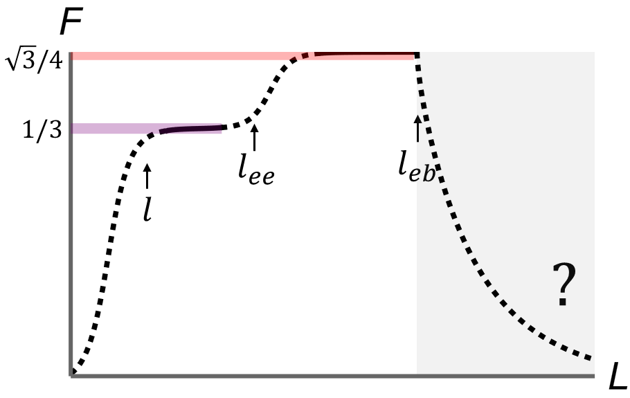
(a)

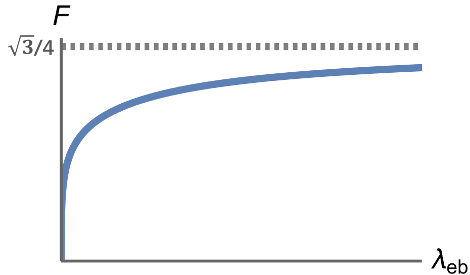
(b)

Figure 1: (a) Schematic plot of the Fano factor ($F$) as a function of system size $L$, initially derived based on a Fermi gas experiencing electron-electron and electron-phonon scattering Steinbach et al. (1996); Nagaev (1995); Beenakker and Buttiker (1992); Shimizu and Ueda (1992). With the phonons taken as in equilibrium on its own, the electron-phonon coupling equilibrates the electron distribution and, thus, reduces the Fano factor, when the system size $L$ exceeds the scattering lengths $l_{eb}$. Here we ask what happens if the bosons are not assumed to be in equilibrium. (b) Schematic result for the Fano factor as a function of the electron-boson coupling, $\lambda_{eb}$, when the bosons are allowed to be out of equilibrium.

To further sharpen the considerations, here we study shot noise in coupled electron-boson systems. We take cue from the known result about the effect of electron-phonon scattering when the phonons are in equilibrium on their own as illustrated in Fig. 1(a): when this scattering is operative, which happens when the corresponding scattering length $l_{eb}$ falls below the system size $L$, the electron-phonon coupling equilibrates the electron distribution and, thus, reduces the Fano factor Nagaev (1995); Steinbach et al. (1996); Beenakker and Buttiker (1992); Shimizu and Ueda (1992). While this phonon-based mechanism per se was ruled out for YbRh₂Si₂ through measurements of long wires Chen et al. (2023), it provides a concrete setting for addressing the following question: What happens to the shot noise in coupled electron-boson systems when the bosons can be driven out of equilibrium through their coupling with the electrons? This question is relevant for the electron-boson problem in the boson-drag regime, where the momentum or energy transferred from the electrons to the boson component can be transferred back to the electron component. While the drag effect for the electron-phonon problem is negligible except for extreme low temperatures, it is expected to be important for the cases where the bosons are collective modes of the electron system due to a large electron-boson coupling (which traces back to the bare electron-electron Coulomb repulsion). The latter case applies to the quantum criticality in the Hertz-Millis-based description Lee (2018); Sur and Lee (2015); Metlitski and Sachdev (2010). In this scenario, in the clean limit, only specific sections of the Fermi surface lose quasiparticle-like behavior (the so-called “hot-spots”) Hlubina and Rice (1995); Rosch (1999) whereas the Fermi liquid description remains valid across the remainder of the Fermi surface, dominating transport properties and leaving the Fano factor intact. In contrast, zero momentum order parameter fluctuations – the kind relevant for ferromagnetism, Ising-nematic and excitonic orders – render the entire Fermi surface “hot”  Lee (2018), even though their contributions to the electrical resistivity is expected to be superlinear in temperature. It is desirable to construct the Boltzmann-Langevin equations suitable for the study of shot noise in coupled electron-boson systems without assuming equilibrium bosons. Here, we do so and determine the shot noise. Our key conclusion is that a sufficiently strong electron-boson coupling restores the Fano factor to $F=\sqrt{3}/4$, as illustrated in Fig. 1(b). Our results support the suggestion Chen et al. (2023); Wang et al. (2022) that quantum criticality of beyond the Landau form Si et al. (2001); Coleman et al. (2001); Senthil et al. (2004) underlies the suppressed shot noise in YbRh₂Si₂, in a similar way that it causes a violation of the Wiedemann-Franz law Pfau et al. (2012).

Transport in electron-boson systems:

Here, we consider metals with two distinct interacting degrees of freedom, one fermionic (electrons; $\psi$) and the other bosonic (phonons, collective soft modes, etc.; $\phi$), with their interaction modeled by a Yukawa term, $\phi\psi^{\dagger}\psi$  A universal description of the system in the presence of an external electromagnetic field, $\bm{E}$, which acts as a source terms, is given by

$$S=\int\differential{\tau}\differential{\bm{r}}\quantity{\mathcal{L}[\psi,\phi]+V(\bm{r})\psi^{\dagger}\psi+ie\bm{A}(\tau,\bm{r})\cdot\psi^{\dagger}\gradient\psi},$$ (1)

where $\mathcal{L}[\psi,\phi]=\psi^{\dagger}\quantity[\partial_{\tau}-H_{0}(\gradient)]\psi-\phi^{\dagger}\quantity[\partial_{\tau}^{2}+c^{2}\nabla^{2}]\phi+\phi\psi^{\dagger}g(\gradient)\psi+u_{\psi}\quantity(\psi^{\dagger}\psi)^{2}+u_{\phi}|\phi|^{4}$, $V(\bm{r})$ is a random potential with $\expectationvalue{V(\bm{r})V(\bm{r}^{\prime})}\propto\delta(\bm{r}-\bm{r}^{\prime})$ which is responsible for elastic scatterings among the electrons, $g(\gradient)$ is a coupling function that controls the interaction between $\psi$ and $\phi$, $\bm{A}$ is an external electromagnetic field such that the applied electric field $\bm{E}=-\partial_{t}\bm{A}$. We will work in the regime where the self-interaction among the bosons is weak; henceforth, we set $u_{\phi}=0$ and simplify notation by setting $u_{\psi}\to u$. The diagrammatic representation of the remaining vertices is shown in Appendix C. Here, the source of the Yukawa vertex is the four-fermion interaction channel that produces soft collective modes as the system is tuned towards a quantum critical point. The remaining four-fermion interaction channels are represented by the $u(\psi^{\dagger}\psi)^{2}$ term. Thus, away from the critical point, while both interaction channels suppress the quasiparticle weight, the development of non-Fermi liquid correlations solely result from the Yukawa vertex Lee (2018).

dia4 (80,50) i1 o1 v14 phantom, tension=0.8i1,v1 plain, left=0.18, tension=0.v2,v1 fermion, left=0.18, tension=0.v3,v2 fermion, tension=0.v4,v3 dots, tension=0.v5,v4 fermion, tension=0.v6,v5 fermion, left=0.18, tension=0.v7,v6 plain, left=0.18, tension=0.v8,v7 plain, left=0.18, tension=0.v9,v8 fermion, left=0.18, tension=0.v10,v9 fermion, tension=0.v11,v10 dots, tension=0.v12,v11 fermion, tension=0.v13,v12 fermion, left=0.18, tension=0.v14,v13 plain, left=0.18, tension=0.v1,v14 photon, tension=0.v3,v13 photon, tension=0.v6,v10 phantom, tension=0.8v6,o1 decor.shape=circle,decor.filled=empty, decor.size=0.1inv1 decor.shape=circle,decor.filled=empty, decor.size=0.1inv8

(a)

dia5 (80,50) i1 o1 v14 phantom, tension=0.8i1,v1 plain, left=0.18, tension=0.v2,v1 fermion, left=0.18, tension=0.v3,v2 photon, tension=0.v3,v4 photon, tension=0.v4,v5 photon, tension=0.v5,v6 fermion, left=0.18, tension=0.v7,v6 plain, right=0.18, tension=0.v7,v8 plain, right=0.18, tension=0.v8,v9 fermion, left=0.18, tension=0.v10,v9 photon, tension=0.v10,v11 photon, tension=0.v11,v12 photon, tension=0.v12,v13 fermion, left=0.18, tension=0.v14,v13 plain, right=0.18, tension=0.v14,v1 fermion, tension=0.v13,v3 fermion, tension=0.v6,v10 phantom, tension=0.8v6,o1 decor.shape=circle,decor.filled=empty, decor.size=0.1inv1 decor.shape=circle,decor.filled=empty, decor.size=0.1inv8

(b)

dia6 (60,60) thick i1 o1,o2 phantomi1,v1 fermion, tension=0.4o1,v1 fermion, tension=0.4v1,o2 decor.shape=circle,decor.filled=shaded, decor.size=1emv1

(c)

dia7 (60,60) thick i1 o1,o2 phantomi1,v1 boson, tension=0.4v1,o1 boson, tension=0.4o2,v1 decor.shape=circle,decor.filled=hatched, decor.size=1emv1

(d)

Figure 2: Scattering processes contributing to the electrical conductivity. In diagrams of type (a) the external frequency-momentum can be carried entirely by electronic propagators. Here, one or more of the boson lines can be exchanged for the dashed lines representing four-fermion vertices [c.f. Appendix C]. For diagrams of type (b), both virtual bosons and electrons carry external frequency-momentum. These processes become important in the drag regime, as explained in the text. (c) and (d) are the renormalized current vertices that capture the scattering of electrons and bosons by the external photon, the thick straight (wavy) lines represent the fully renormalized electron (boson) propagators.

The conductivity tensor is given by $\sigma_{ij}=\expectationvalue{(\psi^{\dagger}\partial_{i}\psi)(\psi^{\dagger}\partial_{j}\psi)}$, which receives quantum corrections from the interaction terms in $\mathcal{L}$. Following Holstein Holstein (1964), we compute $\sigma_{ij}$ at finite $g$ and $u$. Two classes of diagrams contribute to $\sigma_{ij}$. The first class of diagrams is exemplified by processes depicted in Figs. 2(a), where the external frequency-momentum can be carried entirely by electronic virtual excitations. The second class of diagrams, represented by Fig. 2(b), constitute scattering processes where the external frequency-momentum must necessarily be carried by both virtual electrons and bosons. As a result, in scattering processes of the former (latter) category the bosons are at equilibrium (out of equilibrium), which makes the latter class of diagrams to become important in the drag regime where both the electrons and the bosons are out of equilibrium Holstein (1964).

While computing $\sigma_{ij}$ in the drag regime, it is convenient to view the renormalizations to the external-source vertex (c.f., Appendix C) as a self consistent solution to a pair of coupled equations for renormalizations to the current-vertices, one for each type of current-vertex in Figs. 2(c) and (d). These equations are represented diagrammatically as

In Eq. (LABEL:eq:coupled-1) the quantum corrections are split into three categories: the first term is the renormalized current vertex for the electrons due to the four-fermion scatterings, the second term contains additional corrections purely due to the Yukawa vertex, and the final term encodes the feedback from the boson-current vertex. Since the bosons are not charged, they do not directly couple with the external gauge field. Consequently, the quantum corrections in Eq. (LABEL:eq:coupled-2) are generated only through the renormalized electron-current vertex. We note that in Eqs. (LABEL:eq:coupled-1) and (LABEL:eq:coupled-2) the propagators are fully dressed by $u$, $g$, and $V$ appearing in (1), which implies that the fermionic excitations that contribute to the above processes are not necessarily quasiparticles. We have assumed that the system is in the regime where the Migdal’s theorem applies such that the vertex corrections from the Yukawa vertex can be neglected and, in addition, the spectral functions contain dispersive peaks.

The coupled equations above can be utilized to obtain a relationship between the electron and boson distribution functions Holstein (1964), as described in Appendix A.

In the limit $\Omega\to 0$, Eqs. (18) and (19) lead to a set of coupled Boltzmann equations for the electrons and bosons with electron-boson ($I_{eb}$) and boson-electron ($I_{be}$) collision integtals. For completeness, we add collision integrals resulting electron-electron ($I_{ee}$), boson-boson ($I_{bb}$), electron-impurity scatterings ($I_{imp}$) and Langevin source $\delta J^{ext}(x,k,t)$  This procedure leads to the following coupled Boltzmann-Langevin equations:

$$\hat{\mathcal{L}_{\psi}}f(x,k)+I_{imp}(x,k)+I_{ee}(x,k)+I_{eb}(x,k)=\delta J^{ext}$$

$$\hat{\mathcal{L}_{\phi}}N(x,q)+I_{bb}(x,q)+I_{be}(x,q)=0$$ (2)

where

$$\hat{\mathcal{L}_{\psi}}f(x,\bm{k})$$

$$=\quantity[\partial_{t}+v_{x}\partial_{x}+(e\bm{E}-\sum_{\bm{k}^{\prime}}U_{\bm{k},\bm{k}^{\prime}}\partial_{x}\delta f_{\bm{k}^{\prime}})\cdot\partial_{\bm{k}}]f(x,\bm{k})$$ (3)

$$\hat{\mathcal{L}_{\phi}}N(x,\bm{q})=(\partial_{t}+c_{x}\partial_{x})N(x,\bm{q})$$ (4)

and $v_{x}=\partial\epsilon_{k}/\partial k_{x}$ and $c_{x}=\partial\omega_{q}/\partial q_{x}$ are the group velocities of the electronic and bosonic excitations, respectively, and the fermion distribution function $f$ here equals $f^{+}$ introduced above. In addition, $U_{\bm{k},\bm{k}^{\prime}}$ describes the effective electron-electron interaction, $\delta J^{ext}$ is the extraneous electronic flux for the description of electronic fluctuations and shot noise Nagaev (1992); Wang et al. (2022). In the correlated regime, where the electron-electron scattering length $l_{ee}$ is much smaller than the system size $L$, strong electron scattering significantly shapes the nonequilibrium fermion distribution. This distribution, which was derived in our previous workWang et al. (2022), has the following form: $f(x,k)=f_{F}(\epsilon_{\bm{k}},T_{e}(x))+eEv_{x}\tau\partial_{\epsilon}f_{F}$, where $f_{F}(\epsilon_{\bm{k}},T_{e})$ is the Fermi Dirac distribution function with the electron energy $\epsilon_{\bm{k}}=\epsilon_{\bm{k}}^{0}+\sum_{\bm{p}^{\prime}}U_{\bm{k},\bm{k}^{\prime}}\delta f_{\bm{k}^{\prime}}$ and temperature $T_{e}$. The first term in this expression, symmetric in momentum space, is critical for determining the characteristics of shot noise, while the second, antisymmetric term predominantly influences the current behavior.

Shot noise:

When the impurity scattering is dominant over inelastic scatterings, the shot noise can be expressed as Wang et al. (2022); Nagaev (1992):

$$S=\frac{4G}{L}\int_{-L/2}^{L/2}dx\int d\epsilon f(x,\epsilon)(1-f(x,\epsilon))=4G\bar{T}_{e}$$ (5)

where $\bar{T}_{e}=\frac{1}{L}\int_{-L/2}^{L/2}dxT_{e}(x)$ is the averaged nonequilibrium temperature. The Fano factor, defined as the ratio between noise and current, could be expressed as follows,

$$F=\frac{S}{2eGV}=2\bar{\Theta}_{e}$$ (6)

where $\bar{\Theta}_{e}\equiv\bar{T}_{e}/eV$ denotes for the dimensionless averaged temperature. In the absence of any electron-boson coupling, the Fano factor $F$ is $1/3$ for non-interacting electronsNagaev (1992) and $\sqrt{3}/4$ for hot electrons with strong electron-electron collisionsNagaev (1995); Kozub and Rudin (1995). It holds true even in the context of a strongly correlated Fermi liquid where the Landau parameters are considered to be large Wang et al. (2022).

When the electron-boson coupling is present, the electrons and bosons will exchange energy and momentum during electron-boson scattering. Consequently, the temperatures of the electrons ($T_{e}$) and bosons ($T_{b}$) evolve, which in turn affects the characteristics of the shot noise. To accurately track this evolution, it is necessary to solve the coupled Boltzmann-Langevin equations for both electrons and bosons. In this study, we consider the case where bosons deviate from global equilibrium due to interactions with nonequilibrium electrons, and assume they achieve local equilibrium in the steady state due to scattering with electrons. This local equilibrium is characterized by a Bose distribution function $n_{B}(\omega,T_{b}(x))$, where $T_{b}(x)$ denotes the locally defined temperature at position $x$ within the sample.

To investigate the evolution of $T_{e}$ and $T_{b}$, we derive the diffusion equations for electrons and bosons. They are obtained by splitting their nonequilibrium distributions into symmetric and antisymmetric part, and substituting equation for the antisymmetric part into symmetric part (for details see the Appendix D):

$$D\partial_{x}^{2}f(\epsilon,T_{e})+I_{eb}=0$$ (7)

$$\partial^{2}_{x}n_{B}(\omega,T_{b})=\frac{d}{c^{2}\tau_{be}}\left(\frac{1}{\tau_{be}}+\frac{1}{\tau_{bb}}\right)[n_{B}(\omega,T_{b})-n_{B}(\omega,T_{e})]$$ (8)

where

$$I_{eb}=\int d\omega M(\omega) [2f(\epsilon,T_{e})-f(\epsilon-\omega,T_{e})-f(\epsilon+\omega,T_{e})]$$

$$[n_{B}(\omega,T_{e})-n_{B}(\omega,T_{b})]$$ (9)

where $M(\omega)=\frac{\lambda_{eb}\omega^{n+d-2}}{2\pi v_{F}\omega_{D}^{n}c^{d-1}}$, $\frac{1}{\tau_{be}}=4\pi N_{F}\lambda_{eb}\frac{c}{v_{F}}\left(\frac{\omega}{\omega_{D}}\right)^{n}$. Here, $d$ is the space dimension, $n=1$ describes the scaling of the Yukawa coupling with Goldstone bosons (e.g. phonons and AFM magnons), and $n=0$ corresponds to the Yukawa coupling with critical bosons (e.g. collective soft modes of the Hubbard-Stratonovich field). The inverse boson-boson scattering time, represented by $1/\tau_{bb}$, is assumed to be negligible relative to $1/\tau_{be}$. Multiplying Eq.(7) with $\epsilon$ and integrate with $\epsilon$, also multiplying Eq.(8) with $\omega^{d-n}$ and integrate with $\omega$, one gets:

$$L^{2}\partial_{x}^{2}\Theta_{e}^{2}+\frac{6}{\pi^{2}}=\gamma_{e}(\Theta_{e}^{d+n+1}-\Theta_{b}^{d+n+1})$$ (10)

$$L^{2}\partial_{x}^{2}\Theta_{b}^{d-n+1}=\gamma_{b}(\Theta_{b}^{d+n+1}-\Theta_{e}^{d+n+1})$$ (11)

where $\Theta_{e(b)}$, the dimensionless temperature for electrons (bosons), and the parameters $\gamma_{e}$ and $\gamma_{b}$ are defined as follows

$$\Theta_{e(b)}=T_{e(b)}/eV;\quad\gamma_{e}=L^{2}/l_{eb}^{2};\quad\gamma_{b}=L^{2}/l_{be}^{2},$$ (12)

with $l_{eb}^{-1}\equiv l_{e\leftarrow b}^{-1}=\sqrt{\frac{6\zeta(d+n+1)\Gamma(d+n+1)}{2\pi^{3}v_{F}c^{d-1}\omega_{D}^{n}D}\lambda_{eb}(eV)^{d+n-1}}$ and $l_{be}^{-1}\equiv l_{b\leftarrow e}^{-1}=\sqrt{\frac{8d\pi^{2}N_{F}^{2}}{v_{F}^{2}\omega_{D}^{2n}}\frac{\zeta(d+n+1)\Gamma(d+n+1)}{\zeta(d-n+1)\Gamma(d-n+1)}\lambda_{eb}^{2}(eV)^{2n}}$. $\zeta(x)$ and $\Gamma(x)$ denote the Riemann zeta function and the Gamma function, respectively. $\gamma_{e(b)}$ are dimensionless quantities that characterize the energy relaxations of electrons (bosons) due to interactions with bosons (electrons), respectively. The terms $l_{eb}$ and $l_{be}$ denote the electron-boson and boson-electron relaxation lengths, respectively. Specifically, $l_{eb}$ measures the distance electrons can travel without energy relaxation due to bosons, and $l_{be}$ similarly applies for bosons relative to electrons. We note that the electron-boson relaxation length $l_{eb}$ differs from the electron-boson scattering length used in the context of resistivity (e.g., Bloch’s law for acoustic phonons), where the latter is derived from the linearized electron-boson collision integral assuming that bosons are in equilibrium. We further note that the ratio $\gamma_{b}/\gamma_{e}\propto\lambda_{eb}$, the electron-boson coupling at the Yukawa vertex.

Multiplying Eq.(11) with $\gamma_{e}/\gamma_{b}$ and sum with Eq.(10), one can get an exact relation between the two temperatures:

$$\Theta_{e}^{2}+\frac{\gamma_{e}}{\gamma_{b}}\Theta_{b}^{d-n+1}=\frac{6}{\pi^{2}}\left[\frac{1}{8}-\frac{1}{2}\left(\frac{x}{L}\right)^{2}\right]$$ (13)

where we utilized the zero temperature conditions at two boundaries: $T_{e}(\pm\frac{L}{2})=T_{b}(\pm\frac{L}{2})=0$. This relation captures the conservation law of heat transfer between electrons and bosons under local equilibrium conditions. Here, the second term in Eq.(13) can be neglected when $\gamma_{e}\ll\gamma_{b}$, corresponding to $l_{be}\ll l_{eb}$. In this regime, the electrons stay hot, resulting in Fano factor $F=\sqrt{3}/4$. Conversely, when $\gamma_{b}\ll\gamma_{e}$, or equivalently $l_{eb}\ll l_{be}$, the temperature of the bosons, $\Theta_{b}\rightarrow 0$. This occurs because in the absence of significant scattering from electrons ($1/\tau_{be}=0$), bosons remain in global equilibrium.

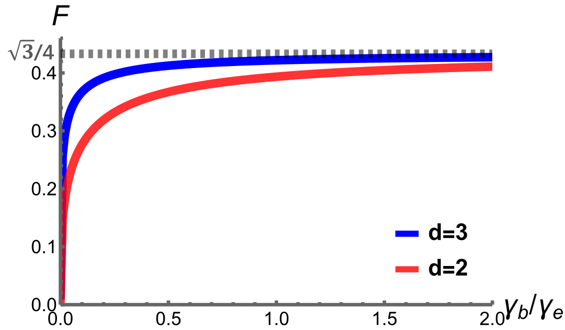
Figure 3: Fano factor $F$ as a function of the ratio $\gamma_{b}/\gamma_{e}\propto\lambda_{eb}$, in the electron-boson drag regime for critical bosons ($n=0$), where $T_{e}(x)=T_{b}(x)$. This regime is characterized by either $\gamma_{e}\gg 1$ or $\gamma_{b}\gg 1$.

We investigate the regime where $\gamma_{e}\gg 1$ or $\gamma_{b}\gg 1$, which arises when the electron-boson or boson-electron scattering is sufficiently strong such that $L\gg l_{eb}$ or $l_{be}$. The strong drag between electrons and bosons equalizes their temperatures, leading to:

$$\Theta_{e}=\Theta_{b}$$ (14)

as seen from Eqn. (10 or (11) at leading order. Under such drag regime, one can get analytic solutions for $\Theta_{e}$ after combining Eq. (14) with Eq. (13). We summarize these results in Table (1) and plot them as functions of $\gamma_{b}/\gamma_{e}$ in Fig. 3. We note that our analytical results are fully supported by the direct numerical solution to Eqs. (10, 11).

$\Theta_{e}^{(d-n)}(x)$	$n=0$	$n=1$
$d=2$	$\Theta^{(2)}\left(\frac{\gamma_{b}}{\gamma_{e}},\Theta_{0e}\right)$	$\sqrt{\frac{\gamma_{b}}{\gamma_{e}+\gamma_{b}}}\Theta_{0e}$
$d=3$	$\frac{1}{\sqrt{2}}\left(\sqrt{\frac{\gamma_{b}^{2}}{\gamma_{e}^{2}}+\frac{4\gamma_{b}}{\gamma_{e}}\Theta_{0e}^{2}}-\frac{\gamma_{b}}{\gamma_{e}}\right)^{\frac{1}{2}}$	$\Theta^{(2)}\left(\frac{\gamma_{b}}{\gamma_{e}},\Theta_{0e}\right)$

Table 1: Table of local temperature for electrons coupled with critical $(n=0)$ and Goldstone $(n=1)$ bosons in two ($d=2$) and three ($d=3$) dimensions in the limit $\gamma_{e}\gg 1$. $\Theta_{0e}(x)=\sqrt{\frac{3}{4\pi^{2}}\left[1-\left(\frac{2x}{L}\right)^{2}\right]}$ is the local temperature of hot electrons without electron-boson couplings, which leads to $F(\lambda_{eb}=0)=\frac{\sqrt{3}}{4}$. The form of $\Theta^{(2)}$ is shown in Appendix E.

Discussion:

Fig. 3 is the central result of our work. Note that $\gamma_{b}/\gamma_{e}\propto\lambda_{\rm eb}$. When the electron-boson coupling $\lambda_{\rm eb}$ is small, $l_{eb}\ll L,l_{be}$, and the Fano factor $F$ goes below $\sqrt{3}/4$. By contrast, when the electron-boson couping is adequately large, as we expect for the cases where the bosons correspond to collective excitations of the electrons, the Fano factor is restored to $\sqrt{3}/4$. This qualitative trend is illustrated in Fig. 1(b).

To summarize, in this paper we study the shot noise in a coupled electron-boson system when the bosons are allowed to go out of equilibrium due to their interactions with the electrons. We construct the coupled Boltzmann-Langevin equations. We show that adequate electron-boson couplings restore the Fano factor to its Fermi liquid value. Our results are important for understanding the reduced shot noise observed in quantum critical heavy fermion metals and beyond, pointing to the quasiparticles being lost from the beyond-Landau form of quantum criticality as the underlying mechanism.

Appendix A Coupled Boltzmann equations

The coupled equations (2,3) of the main text can be utilized to obtain a relationship between the electron and boson distribution functions Holstein (1964),

$$i(\textbf{Q}\cdot\textbf{v}_{k}-\Omega)\Phi_{k}=v_{k}+2\pi\sum_{\textbf{q},\pm}|g_{q}|^{2}\Bigg{[}(\Phi_{k\pm q}-\Phi_{k}\mp n_{q})\left(\frac{f^{\mp}_{F}(\epsilon_{k\pm q}+\Omega)+f^{\mp}_{F}(\epsilon_{k\pm q})}{2}+n_{B}(\omega_{q})\right)\delta(\epsilon_{k}-\epsilon_{k+q}+\omega_{q})$$

$$\qquad+\frac{i}{2\pi}\mathfrak{P}\left(\frac{1}{\epsilon_{k}-\epsilon_{k\pm q}\pm\omega_{q}}\right)\left(f^{\mp}_{F}(\epsilon_{k\pm q}+\Omega)-f^{\mp}_{F}(\epsilon_{k\pm q})\right)(\Phi_{k\pm q}-\Phi_{k})\Bigg{]}$$ (18)

$$i(\textbf{Q}\cdot\nabla_{q}\omega_{q}-\Omega)n_{q}=2\pi\sum_{k}|g_{q}|^{2}\delta(\epsilon_{k}+\omega_{q}-\epsilon_{k+q})\left[-f^{-}_{F}(\epsilon_{k}+\omega_{q})+f^{-}_{F}(\epsilon_{k})\right]\left[\Phi_{k+q}-\Phi_{k}-n_{q}\right].$$ (19)

Here, we have set $\hbar=1$, $v_{k}$ is the magnitude of the renormalized fermion-current vertex due to local coulomb interactions, $(\Omega,\textbf{Q})$ are the frequency-momentum of the external electromagnetic field, $\bm{A}$, $f_{F}^{\pm}(x)$ is the Fermi-Dirac distribution function for the occupied and vacant states, $n_{B}(x)$ is the Bose distribution function, $\Phi_{k}=\quantity[f_{k}-f_{F}^{-}(\epsilon_{k})]/\quantity[eE\partial_{\epsilon_{k}}f_{F}^{-}(\epsilon_{k})]$ and $n_{q}=\quantity[N_{q}-n_{B}(\omega_{q})]/\quantity[eE\partial_{\omega_{q}}n_{B}(\omega_{q})]$ with $f_{k}$ and $N_{q}$ being the full fermion and boson distribution functions, respectively, $\mathfrak{P}(x)$ denotes the principal value, $g_{q}$ is the Fourier components of the Yukawa coupling , and $\epsilon_{k}$ and $\omega_{q}$ are the electron and boson dispersions respectively. We note that the Thomas-Fermi screened temporal part of the electromagnetic gauge field can also participate in Boltzmann transport as an independent bosonic mode. Here, we assume the temperature window is sufficiently smaller than the Thomas-Fermi screening scale, such that the temporal part of the electromagnetic gauge field does not participate in transport. We describe the case when the spectral functions are sharp, though we expect our analysis to remain valid provided that the spectral functions are sharp enough to display dispersive peaks.

In the limit $\Omega\to 0$, Eqs. (18) and (19) leads to a set of coupled Boltzmann equations for the electrons and bosons with electron-boson ($I_{eb}$) and boson-electron ($I_{be}$) collision integtals. For completeness, we add collision integrals resulting electron-electron ($I_{ee}$), boson-boson ($I_{bb}$), , electron-impurity scatterings ($I_{imp}$) and Langevin source $\delta J^{ext}(x,k,t)$ . This leads to the coupled Boltzmann-Langevin equations given in Eq. (4) of the main text.

Appendix B From coupled vertex corrections to Boltzmann equations

In this section we outline the path from Eqs. (18) and (19) in the previous Appendix to the coupled Boltzmann equations. Here, $\Phi_{k}$ and $n_{q}$ parameterize the deviations from the equilibrium fermion and boson distribution functions, respectively,

$$f_{k}=f_{F}^{-}(\epsilon_{k})+eE\Phi_{k}\partial_{\epsilon_{k}}f_{F}^{-}(\epsilon_{k});\qquad N_{q}=n_{B}(\omega_{q})+eEn_{q}\partial_{\omega_{q}}n_{B}(\omega_{q}).$$ (20)

In the limit $\Omega\to 0$ we obtain

$$i\textbf{Q}\cdot\textbf{v}_{k}\Phi_{k}=v_{k}+2\pi\sum_{\textbf{q},s=\pm}W_{s}(k,q)(\Phi_{k+sq}-\Phi_{k}-sn_{q})\left(f^{-s}_{F}(\epsilon_{k+sq})+n_{B}(\omega_{q})\right)$$ (21)

$$i\textbf{Q}\cdot\nabla_{q}\omega_{q}n_{q}=2\pi\sum_{k}W_{+}(k,q)\left[-f^{-}_{F}(\epsilon_{k}+\omega_{q})+f^{-}_{F}(\epsilon_{k})\right]\left[\Phi_{k+q}-\Phi_{k}-n_{q}\right]$$ (22)

where we have defined the transition probability

$$W_{s}(k,q)=2\pi|g_{q}|^{2}\delta(\epsilon_{k}-\epsilon_{k+q}+s\omega_{q})$$ (23)

We multiply both sides of Eq. (21) [Eq. (22)] by $eE\partial_{\epsilon_{k}}f_{F}(\epsilon_{k})$ [$eE\partial_{\omega_{q}}n_{B}(\omega_{q})$], and add $i\textbf{Q}\cdot\textbf{v}_{k}f_{F}$ [$i\textbf{Q}\cdot\textbf{v}_{k}n_{B}$] to obtain the Boltzmann equations in the main text.

Appendix C Bare vertices

Here we specify the bare vertices associated with interaction terms in Eq(1) of the main text.

dia1 (60,40) i1 o1,o2 photon, tension=0.2i1,v1 fermion, tension=0.1o1,v1 fermion, tension=0.1v1,o2

(a)

dia2 (60,40) i1,i2 o1,o2 fermion, tension=0.1i1,v1 fermion, tension=0.1v1,i2 dashes, tension=0.15v1,v2 fermion, tension=0.1o1,v2 fermion, tension=0.1v2,o2

(b)

dia3 (60,40) i1 o1,o2 phantom, tension=0.3i1,v1 fermion, tension=0.1o1,v1 fermion, tension=0.1v1,o2 decor.shape=circle,decor.filled=empty, decor.size=0.1inv1

(c)

Figure 4: Graphical representation of the three vertices that contribute to electrical conductivity. (a) The electron-boson vertex; (b) the four-fermion vertex; (c) the external source vertex representing the direct coupling between an applied electromagnetic field and the electron current.

Appendix D Boltzmann equations for electron-boson coupled systems

We study the coupled Boltzmann equations for electrons and bosons:

$$\mathcal{L}f(x,k)+I_{imp}(x,k)+I_{ee}(x,k)+I_{e-ph}(x,k)=0$$ (24)

$$c_{x}\partial_{x}N(x,q)+I_{ph-ph}(x,q)+I_{ph-e}(x,q)=0$$ (25)

where the collision integrals are given by

$$I_{imp}(x,k)= \sum_{k^{\prime}}W(kk^{\prime})[f(x,k)(1-f(x,k^{\prime}))-f(x,k^{\prime})(1-f(x,k))],$$ (26)

$$I_{ee}(x,k)= \sum_{2,3,4}\widetilde{W}(12;34)\delta_{\bm{k}+\bm{k}_{2},\bm{k}_{3}+\bm{k}_{4}}\delta{(\epsilon+\epsilon_{2}-\epsilon_{3}-\epsilon_{4})}[f_{3}f_{4}(1-f_{1})(1-f_{2})-f_{1}f_{2}(1-f_{3})(1-f_{4})],$$ (27)

$$I_{eb}(x,k)= 2\pi\sum_{\bm{q}}|g_{\bm{q}}|^{2}\left\{[1-f(x,\bm{k})]f(x,\bm{k}+\bm{q})[1+N(x,\bm{q})]-f(x,\bm{k})[1-f(x,\bm{k}+\bm{q})]N_{\lambda}(x,\bm{q})\right\}\delta(\epsilon_{\bm{k}}+\omega_{\bm{q}\lambda}-\epsilon_{\bm{k+q}})$$

$$+|g_{\bm{q}}|^{2}\left\{[1-f(x,\bm{k})]f(x,\bm{k}+\bm{q})N(x,-\bm{q})-f(x,\bm{k})[1-f(x,\bm{k}+\bm{q})][1+N_{\lambda}(x,\bm{q})]\right\}\delta(\epsilon_{\bm{k}}-\omega_{\bm{-q}\lambda}-\epsilon_{\bm{k-q}})$$ (28)

$$I_{be}(x,q)= 4\pi\sum_{\bm{k}}|g_{\bm{q}}|^{2}\left\{[1+N(x,\bm{q})]f(x,\bm{k}+\bm{q})[1-f(x,\bm{k})]-N(x,\bm{q})[1-f(x,\bm{k}+\bm{q})]f(x,\bm{k})\right\}\delta(\epsilon_{\bm{k+q}}-\omega_{\bm{q}\lambda}-\epsilon_{\bm{k}}),$$ (29)

and $c_{x}=\frac{\partial\omega_{q}}{\partial q_{x}}=\frac{cq_{x}}{q}$ is the group velocity of bosons. In these collision integals, $W(pp^{\prime})$ and $\widetilde{W}(12;34)$ are the scattering probability for electron-impurity and electron-electron collisions respectively, and $|g_{q}|^{2}=\lambda_{eb}\left(\frac{\omega}{\omega_{D}}\right)^{n}$, where $n=1$ denotes for the Yukawa coupling with Goldstone bosons (e.g. phonons and AFM magnons), and $n=0$ denotes for the Yukawa coupling with critical bosons (e.g. collective soft modes of the Hubbard-Stratonovich field).

When $l_{ee}\ll L$, the Fermi distribution has the following local equilibrium form:

$$f(x,\bm{k})=f_{F}(\epsilon_{\bm{k}},T_{e}(x))+e\bm{E}\cdot\bm{v}_{\bm{k}}\tau\frac{\partial f_{F}}{\partial\epsilon_{k}}\approx f_{F}(\epsilon_{\bm{k}}-e\bm{E}\cdot\bm{v}_{\bm{k}}\tau,T_{e}(x))$$ (30)

For simplicity, we assume the velocity of fermions is equal to the Fermi velocity $v_{k}=v_{F}$.

The form of $I_{be}$ can be simplified with the help of Eqn.30,

$$I_{be}(x,q)= 4\pi|g_{q}|^{2}[n_{B}(\omega_{q},T_{e}(x))-N(x,q)]\sum_{k}[f(\epsilon_{k}-eEv_{F}\tau)-f(\epsilon_{k}+\omega_{q}-eEv_{F}\tau)]\delta(\epsilon_{\bm{k+q}}-\omega_{\bm{q}\lambda}-\epsilon_{\bm{k}})$$ (31)

$$= 4\pi N_{F}|g_{q}|^{2}\frac{c}{v_{F}}[n_{B}(\omega_{q},T_{e})-N(x,q)]$$ (32)

where

$$\sum_{k}[f(\epsilon_{k})-f(\epsilon_{k+q})]\delta(\omega-\epsilon_{k+q}+\epsilon_{k})=-\frac{1}{\pi}Im[\sum_{k}\frac{1}{\omega-\epsilon_{k+q}+\epsilon_{k}+i\delta}]=N_{F}\frac{\omega}{v_{F}q}$$ (33)

The nonequilibrium boson distribution can be split into even and odd sectors:

$$N(x,q)=N_{even}(x,q)+N_{odd}(x,q)$$ (34)

where $N_{even}=n_{B}(\omega_{q},T_{e})$ preserves under $q\rightarrow-q$, and $N_{odd}(x,q)=-N_{odd}(x,-q)$. Due to different parities, the boson Boltzmann equation is split into two equations:

$$c_{x}\partial_{x}N_{odd} =-[n_{B}(\omega_{q},T_{e})-N_{even}(x,q)]/\tau_{ph-e}$$ (35)

$$c_{x}\partial_{x}N_{even} =N_{odd}(x,q)(\frac{1}{\tau_{be}(q)}+\frac{1}{\tau_{bb}(q)})$$ (36)

with $1/\tau_{be}=4\pi N_{F}|g_{q}|^{2}\frac{c}{v_{F}}=4\pi N_{F}\lambda_{eb}\frac{c\omega^{n}}{v_{F}\omega_{D}^{n}}$. Combining Eqs.(35,36), one get

$$c_{x}^{2}\partial_{x}^{2}n_{B}(\omega_{q},T_{b}(x))=\frac{1}{\tau_{be}}\left(\frac{1}{\tau_{be}}+\frac{1}{\tau_{bb}}\right)[n_{B}(\omega_{q},T_{b}(x))-n_{B}(\omega_{q},T_{e}(x))]$$ (37)

where $c_{x}=\frac{\partial\omega_{q}}{\partial q_{x}}=\frac{cq_{x}}{q}$, $c^{2}_{x}=\frac{1}{d}c^{2}$.

On the other hand, from the electron side, the collision integral can be simplified at leading order (we do not consider Umklapp scattering: $\bm{G}=0$),

$$I_{eb}(x,k)= 2\pi\sum_{\bm{q}}|g_{\bm{q}}|^{2}\left\{[1-f(x,\bm{k})]f(x,\bm{k}+\bm{q})[1+N(x,\bm{q})]-f(x,\bm{k})[1-f(x,\bm{k}+\bm{q})]N_{\lambda}(x,\bm{q})\right\}\delta(\epsilon_{\bm{k}}+\omega_{\bm{q}\lambda}-\epsilon_{\bm{k+q}})$$

$$+|g_{\bm{q}}|^{2}\left\{[1-f(x,\bm{k})]f(x,\bm{k}+\bm{q})N(x,-\bm{q})-f(x,\bm{k})[1-f(x,\bm{k}+\bm{q})][1+N_{\lambda}(x,\bm{q})]\right\}\delta(\epsilon_{\bm{k}}-\omega_{\bm{-q}\lambda}-\epsilon_{\bm{k-q}})$$ (38)

$$= \int d\omega M(\omega)\left\{[1-f(\epsilon_{\bm{k}},T_{e})]f(\epsilon_{\bm{k}}+\omega,T_{e})[1+n_{B}(\omega,T_{b})]-f(\epsilon_{\bm{k}},T_{e}))[1-f(\epsilon_{\bm{k}}+\omega,T_{e})]n_{B}(\omega,T_{b})\right.$$

$$\left.+[1-f(\epsilon_{\bm{k}},T_{e})]f(\epsilon_{\bm{k}}-\omega,T_{e})N(\omega,T_{b})-f(\epsilon_{\bm{k}},T_{e})[1-f(\epsilon_{\bm{k}}-\omega,T_{e})][1+N(\omega,T_{b})]\right\}$$ (39)

$$= \int d\omega M(\omega)[2f(\epsilon_{\bm{k}},T_{e})-f(\epsilon_{\bm{k}}-\omega,T_{e})-f(\epsilon_{\bm{k}}+\omega,T_{e})][n_{B}(\omega,T_{e})-n_{B}(\omega,T_{b})],$$ (40)

where

$$M(\omega)=2\pi\int\frac{d^{d}\bm{q}}{(2\pi)^{d}}|g_{q}|^{2}\delta(\omega-\omega_{q})\delta(\epsilon_{k}+\omega_{q}-\epsilon_{k+q}).$$ (41)

For parabolic electronic bands we have,

$$\omega_{q}+\epsilon_{k}-\epsilon_{k+q}=(c-v_{F}\cos\theta)q+\frac{q^{2}}{2m}.$$ (42)

The form of $M(\omega)$ is dimensionality dependent. For small $\bm{q}$ in three dimensions

$$M(\omega)=\frac{1}{2\pi}\frac{\lambda}{v_{F}c^{2}\omega_{D}^{n}}\omega^{n+1},$$ (43)

while in two dimensions

$$M(\omega)=\frac{1}{2\pi}\frac{\lambda\omega}{v_{F}c\sin(\arccos{(c/v_{F})})}\approx\frac{1}{2\pi}\frac{\lambda\omega^{n}}{v_{F}c\omega_{D}^{n}}.$$ (44)

We can also split the non-equilibrium Fermi distribution function into even and odd sectors:

$$f(x,k)=f_{even}(x,k)+f_{odd}(x,k),$$ (45)

where $f_{even}=f_{F}(\epsilon,T_{e}(x))$, $f_{odd}=eEv_{F}\tau\partial_{\epsilon}f_{F}(\epsilon,T_{e})$, and $\tau$ denotes the electron-impurity scattering time. After combining the even and odd sectors of the Boltzmann equations Wang et al. (2022), we get the following coupled electron-boson diffusion equations:

$$D\partial_{x}^{2}f(\epsilon,T_{e})+I_{e-ph}=0$$ (46)

$$\partial^{2}_{x}n_{B}(\omega,T_{b})=d(4\pi N_{F}\lambda/v_{F}\omega_{D}^{n})^{2}\omega^{2n}[n_{B}(\omega,T_{b}(x))-n_{B}(\omega,T_{e}(x))].$$ (47)

Appendix E Analytic expression of $\Theta_{e}$ in the drage regime

In the electron-boson drag regime, the bosons and electrons share the same temperatures: $\Theta_{e}=\Theta_{b}$. After combining with Eq.(13) and Eq.(14) in the main text,

$$\Theta_{e} =\Theta_{b}$$ (48)

$$\Theta_{e}^{2}+\frac{\gamma_{e}}{\gamma_{b}}\Theta_{b}^{d-n+1} =\frac{6}{\pi^{2}}\left[\frac{1}{8}-\frac{1}{2}\left(\frac{x}{L}\right)^{2}\right]$$ (49)

one can solve $\Theta_{e}$ with different dimension $d$ and scaling exponent $n$ in Yukawa coupling as functions of $p=\gamma_{b}/\gamma_{e}$ and $\Theta_{0e}(x)=\sqrt{\frac{3}{4\pi^{2}}\left[1-\left(\frac{2x}{L}\right)^{2}\right]}$:

• $d=2,n=1$:

  $$\Theta_{e}(p,\Theta_{0e})= \sqrt{\frac{p}{1+p}}\Theta_{0e}$$ (50)

• $d=3,n=0$:

  $$\Theta_{e}(p,\Theta_{0e})=\frac{1}{\sqrt{2}}\sqrt{\sqrt{p^{2}+4p\Theta_{0e}^{2}}-p}$$ (51)

• $d=2,n=0$ and $d=3,n=1$:

  $$\Theta_{e}(p,\Theta_{0e})=\frac{1}{3}\left(-p+\frac{2^{1/3}p^{2}}{\left(27\Theta_{0e}^{2}p-2p^{3}+3\sqrt{81\Theta_{0e}^{4}p^{2}-12\Theta_{0e}^{2}p^{4}}\right)^{1/3}}+\frac{\left(27\Theta_{0e}^{2}p-2p^{3}+3\sqrt{81\Theta_{0e}^{4}p^{2}-12\Theta_{0e}^{2}p^{4}}\right)^{1/3}}{2^{1/3}}\right)$$ (52)