Generative Subspace Adversarial Active Learning for Outlier Detection in Multiple Views of High-dimensional Data
Abstract
Outlier detection in high-dimensional tabular data is an important task in data mining, essential for many downstream tasks and applications. Existing unsupervised outlier detection algorithms face one or more problems, including inlier assumption (IA), curse of dimensionality (CD), and multiple views (MV). To address these issues, we introduce Generative Subspace Adversarial Active Learning (GSAAL), a novel approach that uses a Generative Adversarial Network with multiple adversaries. These adversaries learn the marginal class probability functions over different data subspaces, while a single generator in the full space models the entire distribution of the inlier class. GSAAL is specifically designed to address the MV limitation while also handling the IA and CD, being the only method to do so. We provide a comprehensive mathematical formulation of MV, convergence guarantees for the discriminators, and scalability results for GSAAL. Our extensive experiments demonstrate the effectiveness and scalability of GSAAL, highlighting its superior performance compared to other popular OD methods, especially in MV scenarios.
1 Introduction
Outlier detection (OD), a fundamental and widely recognized issue in data mining, involves the identification of anomalous or deviating data points within a dataset. Outliers are typically defined as low-probability occurrences within a population Wang et al. (2019); Han et al. (2022). In the absence of access to the true probability distribution of the data points, OD algorithms rely on the construction of a scoring function. Points with higher scores are more likely to be outliers. As we will elaborate, existing unsupervised OD algorithms are susceptible to one or more of the following problems, in high-dimensional tabular data scenarios in particular.
-
•
The inlier assumption (IA): OD algorithms may make assumptions about what constitutes an inlier, which can be challenging to verify and validate Liu et al. (2020).
-
•
The curse of dimensionality (CD): As the dimensionality of data increases, the challenge of identifying outliers intensifies, often resulting in a diminished effectiveness of certain OD algorithms Bellman (1957).
-
•
Multiple Views (MV): This alludes to the fact that outliers often are only visible in certain ”views” of the data and are hidden in the full space of original features Müller et al. (2012).
We now explain these problems one by one.
The inlier assumption poses a challenge to algorithms that assume a standard profile of the inlier data. For example, angle-based algorithms like ABOD Kriegel et al. (2008) assume that inliers have other inliers at all angles. Similarly, neighbor-based algorithms like kNN Ramaswamy et al. (2000) assume that inliers have other neighboring data nearby. These assumptions influence the scoring process, which is determined by measuring the degree to which a sample diverges from this assumed norm. While these algorithms can be effective under their specific assumptions, their performance can degrade when these assumptions do not hold Liu et al. (2020). Ideally, a method should be free of any reliance on inlier assumptions for more robust applicability.
The curse of dimensionality Bellman (1957) refers to the decrease in the relative proximity of data points as the number of dimensions increases. Simply put, as it increases, the distinctiveness of each point’s location decreases, making distances between points less meaningful. This effect is particularly problematic for OD algorithms that rely on distances or on identifying neighbors to detect outliers, such as density- (e.g., LOF Breunig et al. (2000)), neighbor- (e.g., kNN Ramaswamy et al. (2000)), and cluster-based (e.g., SVDD (Aggarwal, 2017, Chapter 2)) OD algorithms.
Multiple Views refers to the phenomenon that certain complex correlations between features are only observable in some feature subspaces Müller et al. (2012). As detailed in Aggarwal (2017), this occurs when the dataset contains additional irrelevant features, making some outliers only detectable in certain subspaces. In scenarios where multiple subspaces contain different interesting structures, this problem is exacerbated. It then becomes increasingly difficult to explain the variability of a data point based solely on its behavior in a single subspace Keller et al. (2013). This problem is different from the curse of dimensionality as it can occur independently of the dimensionality of the dataset, and it can be mitigated with more data points. We showcase all the presented issues of a detector in the following example:
Example 1 (Effect of MV, IA and CD).
Consider the random variables and , where and are highly correlated and is just Gaussian noise. Figure 1 contains plots with different numbers of realizations for . We also plotted the classification boundaries from both a locality-based method (green) and a cluster-based method (red) in the subspace. If one fits the cluster-based detector in the full space of the data, the outlier shown in the figure (red cross) would not be detectable. However, the outlier is always detectable in the subspace, as we can see. Once we increase the number of samples over , the method detects the outlier in the full space (MV). On the contrary, the locality-based method could not detect the outlier in any tested scenario (MV + IA). If we increase the dimensionality by adding more features consisting of noise, no method can detect the outlier in the full space (MV + IA + CD).
We are interested in tackling outlier detection whenever a population exhibits MV, like Müller et al. (2012); Keller et al. (2013); Kriegel et al. (2009) and as showcased in Aggarwal (2017). Particularly, the goal of this paper is to propose the first outlier detection method that explicitly addresses IA, CD, and MV simultaneously.
As we will explain in the next section, we build on Generative Adversarial Active Learning (GAAL) Zhu and Bento (2017), a widely used approach for outlier detection Liu et al. (2020); Guo et al. (2021); Sinha et al. (2019). It involves training a Generative Adversarial Network (GAN) to mimic the distribution of outlier data, and it enhances the discriminator’s performance through active learning Settles (2009), leveraging the GAN’s data generation capability. GAAL methods avoid IA Liu et al. (2020) and use the multi-layered structure of the GAN to overcome the curse of dimensionality Poggio et al. (2020). However, they may miss important subspaces, leading to the multiple views problem. Extending GAAL to also address MV is not immediately obvious.
Challenges.
Addressing the Multiple Views problem by training a feature ensemble of GAN-based models is not trivial. (1) The joint training of generators and discriminators in GANs requires careful monitoring to determine the optimal stopping point, a task that becomes daunting for large ensembles. (2) The generation of difficult-to-detect points in a subspace remains hard Steinbuss and Böhm (2017). While several authors have proposed multi-adversarial architectures for GANs Durugkar et al. (2016); Choi and Han (2022), none of them specifically address adversaries tailored to subspaces composed of feature subsets. Furthermore, these methods may not be suitable for GAAL since they do not have convergence guarantees for detectors, as we will explain.
Contributions.
(1) We propose GSAAL (Generative Subspace Adversarial Active Learning), a novel GAAL method that uses multiple adversaries to learn the marginal class probability functions in different data subspaces. Each adversary focuses on a single subspace. Simultaneously, we train a single generator in the full space to approximate the entire distribution of the inlier class. (2) By giving the first mathematical formulation of the “multiple views” issue, we showed GSAAL’s ability to mitigate the MV problem. (3) We formulate the novel optimization problem for GSAAL and give convergence guarantees of each discriminator to the marginal distribution of their respective subspace. Additionally, we give complexity results for the scalability of our method. (4) Through extensive experimentation, we corroborated our claims regarding scalability and suitability for MV. (5) We tested our method on the one-class classification task (novelty detection) for outlier detection using 22 popular benchmark datasets. GSAAL outperformed all popular OD algorithms from different families and is orders of magnitude faster in inference than its best competitor. (6) Our code for the experiments and all examples is publicly available.111https://github.com/WamboDNS/GSAAL
2 Related Work
| Type | IA | CD | MV |
|---|---|---|---|
| Classical | ✗ | ✗ | ✗ |
| Subspace | ✗ | ✓ | ✓ |
| Generative w/ uniform distribution | ✓ | ✗ | ✗ |
| Generative w/ param. distribution | ✗ | ✓ | ✗ |
| Generative w/ subspace behavior | ✗ | ✓ | ✓ |
| GAAL | ✓ | ✓ | ✗ |
| GSAAL (Our method) | ✓ | ✓ | ✓ |
This section is a brief overview of popular unsupervised outlier detection methods related to our approach. We categorize them based on their ability to address the specific limitations outlined above. Table 1 is a comparative summary.
2.0.1 Classical Methods
Conventional outlier detection approaches, such as distance-based strategies like LOF and KNN, angle-based techniques like ABOD, and cluster-based methods like SVDD, rely on specific assumptions on the behavior of inlier data. They use a scoring function to measure deviations from this assumed norm. These methods face the inlier assumption limitation by definition. For example, local methods that assume isolated outliers fail when several outlying samples fall together. In addition, many classical methods, which rely on measuring distances, are susceptible to the curse of dimensionality. Both limitations impair the effectiveness and efficiency of these methods Liu et al. (2020).
2.0.2 Subspace Methods
Subspace-based methods Kriegel et al. (2009) operate in lower-dimensional subspaces formed by subsets of features. They effectively counteract the curse of dimensionality by focusing on identifying so-called “subspace outliers” Keller et al. (2012). These outliers, which are prevalent in high-dimensional datasets with many correlated features, are often elusive to conventional non-subspace methods Liu et al. (2008); Müller et al. (2012). However, existing subspace methods inherently operate on specific assumptions on the nature of anomalies in each subspace they explore, and thus face the inlier assumption limitation.
2.0.3 Generative Methods
A common strategy to mitigate the IA and CD limitations is to reframe the task as a classification task using self-supervision. A prevalent self-supervised technique, particularly for tabular data, is the generation of artificial outliers El-Yaniv and Nisenson (2006); Liu et al. (2020). This method involves distinguishing between actual training data and artificially generated data drawn from a predetermined “reference distribution”. Hempstalk et al. (2008) showed that by approximating the class probability of being a real sample, one approximates the probability function of being an inlier. One then uses this approximation as a scoring function Liu et al. (2020). However, it is not easy to find the right reference distribution, and a poor choice can affect OD by much Hempstalk et al. (2008).
A first approach to this challenge proposed the use of naïve reference distributions by uniformly generating data in the space. This approach showed promising results in low-dimensional spaces but failed in high dimensions due to the curse of dimensionality Hempstalk et al. (2008). Other approaches, such as assuming parametric distributions for inlier data (Aggarwal, 2017, Chapter 2) or directly generating in susbpaces Désir et al. (2013), can avoid CD when the parametric assumptions are met. Methods that generate in the subspaces can model the subspace behavior, additionally tackling the MV limitation. However, these last two approaches do not address the IA limitation, as they make specific assumptions about the behavior of the inlier data.
2.0.4 Generative Adversarial Active Learning
According to Hempstalk et al. (2008), the closer the reference distribution is to the inlier distribution, the better the final approximation to the inlier probability function will be. Hence, recent developments in generative methods have focused on learning the reference distribution in conjunction with the classifier. A key approach is the use of Generative Adversarial Networks (GANs), where the generator converges to the inlier distribution Goodfellow et al. (2014). The most common approaches for this are GAAL-based methods Liu et al. (2020); Guo et al. (2021); Sinha et al. (2019). These methods differentiate themselves from other GANs for OD by training the detectors using active learning after normal convergence of the GAN Schlegl et al. (2017); Donahue et al. (2017). The architecture of GAAL inherently addresses the curse of dimensionality, as GANs can incorporate layers designed to manage high-dimensional data Poggio et al. (2020). In practice, GAAL-based methods outperformed all their competitors in their original work. However, they overlook the behavior of the data in subspaces and therefore may be susceptible to MV.
Our method, GSAAL, incorporates several subspace-focused detectors into GAAL. These detectors approximate the marginal inlier probability functions of their subspaces. Thus, GSAAL effectively addresses MV while inheriting GAAL’s ability to overcome IA and CD limitations.
3 Our Method: GSAAL
We first formalize the notion of data exhibiting multiple views. We then use it to design our outlier detection method, GSAAL, and give convergence guarantees. Finally, we derive the runtime complexity of GSAAL. All the proofs and extra derivations can be found in the technical appendix.
3.1 Multiple Views
Several authors Aggarwal (2017); Müller et al. (2012); Keller et al. (2013); Kriegel et al. (2009); Liu et al. (2008) have observed that at times the variability of the data can only be explained from its behavior in some subspaces. Researchers variably call this problem “the subspace problem” Aggarwal (2017); Kriegel et al. (2009) or “multiple views of the data” Keller et al. (2012); Müller et al. (2012). Previous research has largely focused on practical scenarios, leaving aside the need for a formal definition. In response, we propose a unifying definition of “multiple views” that provides a foundation for developing methods to address this challenge effectively.
The problem “multiple views” of data (MV) arises from two different effects. First, it involves the ability to understand the behavior of a random vector by examining lower-dimensional subsets of its components . Second, it stems from the challenge of insufficient data to obtain an effective scoring function in the full space of . As Example 1 shows, combining these two effects obscures the behavior of the data in the full space. Hence, methods not considering subspaces when building their scoring function may have issues detecting outliers under MV. The next definition formalizes the first effect.
Definition 1 (myopic distribution).
Consider a random vector and , the set of diagonal binary matrices without the identity. If there exists a random matrix , such that
| (1) |
we say that the distribution of is myopic to the views of . Here, and are realizations of and , and and are the pdfs of and .
It is clear that, under MV, using to build a scoring function instead of mitigates the effects. This comes as the subspaces selected by are smaller in dimensionality. Hence it should take fewer samples to approximate the pdf of . The difficulty is that it is not yet clear how to approximate . The following proposition elaborates on a way to do so. It states that by averaging a collection of marginal distributions of in the subspaces given by realizations of , one can approximate the distribution of .
Proposition 1.
Let and be as before with myopic to the views of . Consider a set of independent realizations of : . Then is a sufficient statistic for .
MV appears when there is a lack of data, and its distribution is myopic. To improve OD under MV, one can exploit the distribution myopicity to model in the subspaces, where less data is sufficient. Proposition 1 gives us a way to do so, by approximating . In this way, under myopicity, this also approximates , avoiding MV. Our method, GSAAL, exploits these derivations, as we explain next.
3.2 GSAAL
GAAL methods tackle IA by being agnostic to outlier definition and mitigate CD through the use of multilayer neural networks Liu et al. (2020); Li et al. (2017); Poggio et al. (2020). GAAL methods have two steps:
-
1.
Training of the GAN. Train the GAN consisting of one generator and one detector using the usual - optimization problem as in Goodfellow et al. (2014).
- 2.
After Step 2, the detector converges to . However, our goal is to approximate by exploiting a supposed myopicity of the distribution. We extend GAAL methods to also address MV in what follows. The following theorem adapts the objective function of the GAN to the subspace case and gives guarantees that the detectors converge to the marginal pdfs used in Proposition 1:
Theorem 1.
Consider and as in the previous definition, with a realization of and a set of realizations of . Consider a generator and , , a set of detectors such as . is an arbitrary noise space where randomly samples from. Consider the following optimization problem
| (2) |
where each addend is the binary cross entropy in each subspace. Under these conditions, the following holds:
-
Each detector in optimum is . Thus, in optimum
-
Each individual converges to after trained in Step 2 of a GAAL method.
-
approximates . If is myopic, also approximates .
Using Theorem 1 we can extend the GAAL methods to the subspace case:
-
1.
Training the GAN. Train a GAN with one generator and multiple detectors with Equation (2) as the objective function. The training of each detector stops when the loss reaches its value with the optimum in Statement .
-
2.
Training of the detectors by active learning. Train each as in Step 2 of a regular GAAL method using . By Statement of the Theorem, each will approximate . By Statement , will approximate under the myopicity of the data.
We call this generalization of GAAL Generative Subspace Adversarial Active Learning (GSAAL). The appendix contains the pseudo-code for GSAAL.
3.3 Complexity
In this section, we focus on studying the theoretical complexity of GSAAL. We study both its usability for training and, more importantly, for inference.
Theorem 2.
Consider our GSAAL method with generator and detectors , each with four fully connected hidden layers, nodes in the detectors and in the generator. Let be the training data for GSAAL, with data points and features. Then the following holds:
-
Time complexity of training is . is an unknown complexity variable depicting the unique epochs to convergence for the network in dataset .
-
Time complexity of single sample inference is in , with the number of detectors used.
The linear inference times make GSAAL particularly appealing in situations where the model can be trained once for each dataset, like one-class classification. We build on this particular strength in the following section.
4 Experiments
This section presents experiments with GSAAL. We will outline the experimental setting, and examine the handling of “multiple views” in GSAAL and other OD methods. We then evaluate GSAAL’s performance against various OD methods and investigate its sensitivity to the number of detectors and its scalability. We also added additional experiments with other competitors outside of our related work in the appendix of the article. Our experiments used an RTX 3090 GPU and an AMD EPYC 7443p CPU running Python in Ubuntu 22.04.3 LTS. Deep neural network methods were trained on the GPU and inferred on the CPU; shallow methods used only the CPU.
4.1 Experimental Setting
This section has three parts: First, we describe the synthetic and real data for the outlier detection experiments. Then, we describe the configuration of GSAAL. Finally, we present our competitors.
4.1.1 Datasets
Synthetic.
We constructed synthetic datasets, each containing two correlated features, and , along with 58 independent features , consisting of Gaussian noise. This approach simulates datasets that exhibit the MV property by integrating irrelevant features into a pair of highly correlated variables. We detail the methodology and all different correlation patterns, in the technical appendix.
Real.
We selected 22 real-world tabular datasets for our experiments from Han et al. (2022). The selection criteria included datasets with less than 10,000 data points, more than 10 outliers, and more than 15 features, focusing on high-dimensional data while keeping the runtime (of competing OD methods) tractable. Table 2 contains the summary of the datasets. For datasets with multiple versions, we chose the first in alphanumeric order. Details about each dataset are available in the original source Han et al. (2022).
| Dataset | Category | Dataset | Category |
|---|---|---|---|
| 20news | Text | MNIST | Image |
| Annthyroid | Health | MVTec | Text |
| Arrhythmia | Cardiology | Optdigits | Image |
| Cardiot.. | Cardiology | Satellite | Astronomy |
| CIFAR10 | Image | Satimage-2 | Astronomy |
| F-MNIST | Image | SpamBase | Document |
| Fault | Industrial | Speech | Linguistics |
| InternetAds | Image | SVHN | Image |
| Ionosphere | Weather | Waveform | Elect. Eng. |
| Landsat | Astronomy | WPBC | Oncology |
| Letter | Image | Hepatitis | Health |
4.1.2 Network Settings
Structure.
Unless stated otherwise, GSAAL uses the following network architecture. It consists of four fully connected layers with ReLu activation functions used in the generator and the detectors. Each layer in detectors has nodes, where and are the number of data points and features in the training set, respectively. This configuration ensures linear inference time. The generator has nodes in each layer, a standard in GAAL approaches, which ensures polynomial training times. We assumed to be distributed uniformly across all subspaces. Therefore, we obtained each subspace for the detectors by drawing uniformly from the set of all subspaces.
Training.
Like other GAAL methods Liu et al. (2020); Zhu and Bento (2017), we train the generator together with all the detectors until the loss of stabilizes. Then we train each detector until convergence with fixed. To automate this process, we introduce an early stopping criterion: Training stops when a detector’s loss approaches the theoretical optimum (), see statement of Theorem 1. For consistency across experiments, training parameters remain fixed unless otherwise noted. Specifically, the learning rates of the detectors and the generator are 0.01 and 0.001, respectively. We use minibatch gradient descent Goodfellow et al. (2016) optimization, with a batch size of 500.
4.1.3 Competitors
| Type | Competitors |
|---|---|
| Classical | kNN, LOF, ABOD, SVDD |
| Subspace | Isolation Forest, SOD |
| Gen., uniform dist. | Not included (see the text) |
| Gen., parametric dist. | GMM |
| Gen., subspace behavior | Not included (see the text) |
| GAAL | MO-GAAL |
We selected popular and accessible methods from each category, as summarized in Table 3, guided by related work. We excluded generative methods with uniform distributions because they prove ineffective for large datasets Hempstalk et al. (2008). We could not include a representative for generative methods with subspace behavior due to operational issues with the most relevant method in this class, Désir et al. (2013), caused by its outdated repository.
4.2 Effect of Multiple Views on Outlier Detection
To demonstrate the effectiveness of GSAAL under MV, we use synthetic datasets. Visualizing the outlier scoring function in a 60-dimensional space is challenging, so we project it into the - subspace. A method adept at handling MV should have a boundary that accurately reflects the and dependency structure. The procedure is as follows:
-
1.
Generate a synthetic dataset as described in section 4.1.1 and train the OD model.
-
2.
Using this model, compute the scores for the points and visualize the level curves on the - plane.
Figure 2 shows results for selected datasets and competitors, which are detailed in the Appendix. It shows the level curves and decision boundaries (dashed lines) of the methods. Notably, our model effectively detects correlations in the right subspace. For example, in the banana dataset, GSAAL accurately creates a banana-shaped boundary and outperforms other methods in distinguishing outliers from inliers in this subspace.
4.3 One-class Classification
This section evaluates GSAAL on a one-class classification task Seliya et al. (2021). First, we study the effectiveness of GSAAL on real data. Then, we explore the impact of parameter variations on the model’s performance. Finally, we investigate the scalability of GSAAL in practical scenarios.
4.3.1 Real-world Performance
We perform the outlier detection experiments on real datasets. Specifically, we take on the task of one-class classification, where the goal is to detect outliers by training only on a collection of inliers Han et al. (2022). To evaluate the performance of OD methods, we use AUC as it is resilient to test data imbalance, a common issue in OD tasks . The procedure is as follows:
-
1.
Split the dataset into a training set containing of the inliers from , and a test set containing the remaining inliers and all outliers.
-
2.
Train an outlier detection model with and evaluate its performance on with ROC AUC.
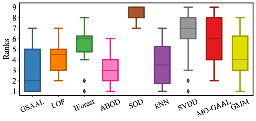
To save space, we moved the detailed AUC results to the appendix; Figure 3 summarizes them. It shows that GSAAL achieves the lowest median rank. Although other subspace methods tend to perform better with irrelevant attributes Liu et al. (2008); Kriegel et al. (2009), they did not outperform classical OD methods on average in our experiments. Notably, ABOD, the second best method in our experiments, performed poorly in the MV tests (Section 4.2).
For statistical comparisons, we use the Conover-Iman post hoc test for pairwise comparisons between multiple populations Conover and Iman (1979). It is superior to the Nemenyi test due to its improved type I error boundings Conover (1999). Conover-Iman test requires a preliminary positive result from a multiple population comparison test, for which we employ the Kruskal-Wallis test Kruskal (1952).
Table 4 shows the test results. In each cell, ‘’ indicates that the method in the row has a significantly lower median rank than the method in the column, while ‘’ indicates a significantly higher median rank. One symbol indicates p-values and two symbols indicate p-values . A blank indicates no significant difference. The table shows that GSAAL is superior to most of its competitors. Our method does not significantly outperform the classical methods ABOD and kNN. However, these methods struggle to detect structures in subspaces, showing their inadequacy in dealing with the MV limitation, see Section 4.2.
Overall, the results support GSAAL’s superiority in outlier detection tasks involving multiple views. Additionally, they establish our method as the leading GAAL option for One-class classification
| Method | ABOD | GSAAL | GMM | IForest | KNN | LOF | MO GAAL | SVDD | SOD |
|---|---|---|---|---|---|---|---|---|---|
| ABOD | = | ++ | ++ | ++ | ++ | ++ | |||
| GSAAL | = | ++ | ++ | + | ++ | ++ | ++ | ||
| GMM | – – | – – | = | ++ | – – | – – | ++ | ++ | |
| IForest | – – | – – | – – | = | – – | ++ | ++ | ||
| KNN | ++ | ++ | = | ++ | ++ | ||||
| LOF | – | ++ | = | ++ | + | ++ | |||
| MO GAAL | – – | – – | – – | – – | – – | = | ++ | ||
| SVDD | – – | – – | – – | – | = | ++ | |||
| SOD | – – | – – | – – | – – | – – | – – | – – | – – | = |
4.3.2 Parameter Sensibility
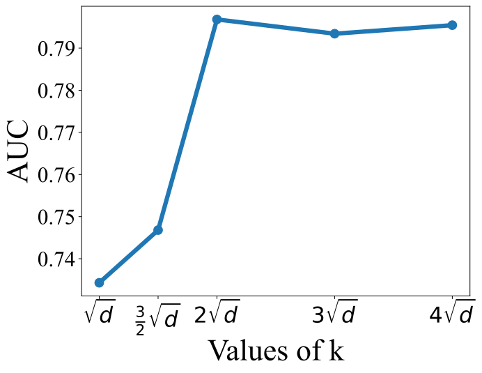
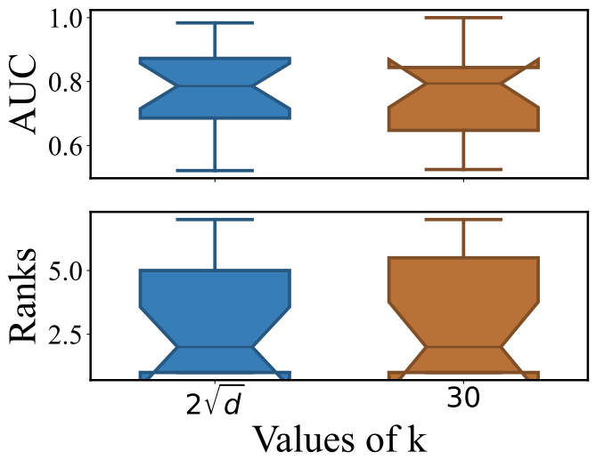
We now explore the effect of the number of detectors in GSAAL, , by repeating the previous experiments with varying . Figure 4(a) plots the median AUC for different values, showing a stabilization at larger . Next, Figure 4(b) compares the results with a fixed and the default value used in the previous experiments; there is no large difference in either the AUC or the ranks. We also found that the results in Table 4 remain almost the same if one sets . So we recommend fixing , which makes GSAAL very suitable for high-dimensional data, as we will show next.
4.3.3 Scalability
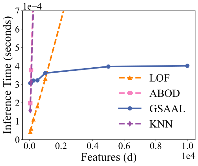
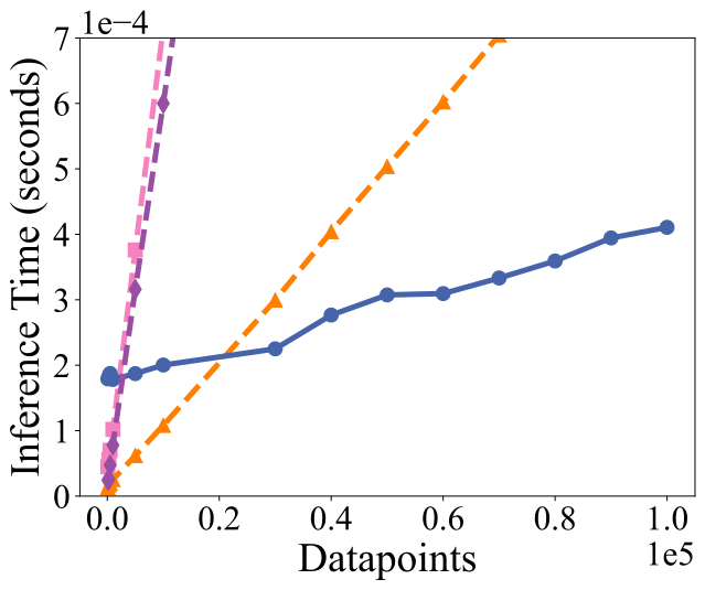
In section 3.3, we derived that the inference time of GSAAL scales linearly with the number of training points if the number of detectors is fixed, while it does not depend on the number of features . This is in contrast to other methods, in particular LOF, KNN, and ABOD, which have quadratic runtimes in Breunig et al. (2000); Kriegel et al. (2008). We now validate this experimentally. The procedure is as follows:
-
1.
Generate datasets and consisting of random points. .
-
2.
Train an OD method using and record the inference time over .
Following the result of the sensitivity study, we fixed . Figure 5(a) plots the inference time of a single data point as a function of the number of features when . Figure 5(b) plots the inference time as a function of the number of points in , for a fixed number of 100 features. Both figures confirm our complexity derivations and show that GSAAL is particularly well-suited for large datasets.
5 Limitations & Conclusions
We now briefly discuss future research directions and acknowledge the limitations of our study. We then summarize the main findings.
5.1 Limitations and Future Work
In section 4 we randomly selected subspaces for training the detectors in GSAAL, i.e. we took a uniform distribution of . This was already sufficient to demonstrate the highly competitive performance of our method. However, GSAAL can work with any subspace search strategy to obtain the distribution of , for example, the methods exploiting multiple views Keller et al. (2013, 2012). We have not included them in this paper due to the lack of an official implementation. In the future, we plan to benchmark various subspace search methods in GSAAL to see if there is one that consistently improves OD performance.
Next, GSAAL is limited to tabular data, since the “multiple views” problem has only been observed for this data type. The mathematical formulation of MV in section 3 does not exclude structured data. The difficulty lies in identifying good search strategies for for non-tabular data, which remains an open question Gupta et al. (2017). However, depending on the type of structured data, extending GSAAL to work with it is not immediate. Therefore, building a method that exploits the theoretical derivations of GSAAL for structured data is future work.
5.2 Conclusions
Unsupervised outlier detection (OD) methods rely on a scoring function to distinguish inliers from outliers, since the true probability function that generated the dataset is usually unavailable in practice. However, they face one or more of the following problems — Inlier Assumption (IA), Curse of Dimensionality (CD), or Multiple Views (MV). In this article, we have proposed the first mathematical formulation of MV, which allows for a better understanding of how to solve this occurrence. Using this formulation, we developed GSAAL, which is the first OD approach that solves MV, CD, and IA. In short, GSAAL is a generative adversarial network with a generator and multiple detectors fitted in the subspaces to find outliers not visible in the full space. In our experiments on 26 different datasets, we demonstrated the usefulness of GSAAL, in particular, its ability to deal with MV and its superior performance on OD tasks with real datasets. In addition, we have shown that GSAAL can scale up to deal with high-dimensional data, which is not the case for our most competent competitors. These results confirm GSAAL’s ability to deal with data exhibiting MV and its usability in any practical scenario involving large datasets.
6 Aknowledgments
This work was supported by the Ministry of Science, Research and the Arts Baden Württemberg, project Algorithm Engineering for the Scalability Challenge (AESC).
Appendix A Theoretical Appendix
A.1 Previous Remarks
Before starting to prove our main results, it is important to add a remark about our notation in this article. Whenever we denote , we mean the operation resulting in the following vector: . Thus, is a random vector following its own distribution . However, it is important to remark that , and therefore, also , does not state the usual matrix-vector multiplication. What we mean by is the operation , where stands for the range-complete version of and the usual matrix multiplication. This means that whenever we write we are considering the projection of into the subspace of the features selected in . This means that is the random vector composed of the features selected by , and therefore, denotes subsequent marginal pdf of . We do not state this in the main text as it functionally does not change anything of our derivations, and simply works as a notation. The only important remarks stemming from this fact are the following:
-
1.
, where denotes the projection of a point into the subspace of . Therefore, we can write .
-
2.
The operator as stated before is not distributive. This is trivial, as given a random matrix as in definition 1, () is defined properly, as . However, denotes the vector subtraction between two vectors with different dimensionality.
While not important to understand the following proofs and the derivations from the main text, understanding this is crucial for anyone seeking to work with these definitions.
A.2 Proofs
We will reformulate all of the statements for completition before introducing each proof.
Proposition 2.
Let and be as before with myopic to the views of . Consider a set of independent realizations of : , a realization of , , and a realization of , . Then is a sufficient statistic for .
Proof.
Consider and as in the statement. Further consider the variable , being the identity matrix. Then, as has its image in , it is clear that Therefore, we can define as the joint pdf of and . Now, recalling the definition of marginal distribution:
Since is defined in a discrete space:
We can approximate this by the sample mean, with a sample of size :
Now, as is perfectly represented by , and vice versa, sampling is equivalent to sampling . We will prove that, . After that, the rest of the proof comes clearly by substituting and recalling that the sample mean is a sufficient estimator of the expected value. First, recall the definition of conditional probability:
Now, by considering that , we have that . Therefore, by the law of total probabilities and the definition of conditional probability:
Thus:
Then, since:
by myopicity, independence of , and considering that sampling from is the same as sampling from , it trivially follows that:
We can retrieve the equality in the statement by consdering to be uniformly distributed —as we do in section 4. ∎
Theorem 3.
Consider and as in the previous definition, with a realization of and a set of realizations of . Consider a generator and , , a set of detectors such as . is an arbitrary noise space where randomly samples from. Consider the following objective function
| (3) |
Under these conditions, the following holds:
-
Each detector’s loss in optimum is .
-
Each individual converges to after trained in Step 2 of a GAAL method.
-
approximates . If is myopic, also approximates .
Proof.
This proof will follow mainly the results in Goodfellow et al. (2014), adapted for our case. We will first derivative two general results that we are going to use to immediately prove and . First, consider the objective function
where is the random vector used by to sample from the noise space . We will write and instead of and as an abuse of notation.
The problem is, then, to optimize:
| (4) |
Fixing and maximizing for all , each detector individually maximizes . Let us try to obtain the optimal of each with a fixed . First, we write:
As uses to sample from its sample distribution , we can rewrite the second addent, like in Goodfellow et al. (2014), as:
Aggregating both integrals, we have a function of the type , with . It is a known fact in calculus that obtains its optimum in . As , obtains its optimum for a given in:
| (5) |
Let us now consider the following function
| (6) |
This is known in Game Theory as the cost function of player “” in the null-sum game defined by the optimization problem. Goodfellow et al. (2014) refers to it as the virtual training criterion of the GAN. The adversarial game defined by (4) reaches an equilibrium (and thus, the problem an optimum) whenever is minimized. We will study the value of in such equilibrium and use it, together with (5), to prove the statements.
Rewriting it is clear that:
This expression corresponds to that of a sum of multiple binary cross entropies between a population coming from and from projected by . Therefore, as we know, we can rewrite:
with the Jensen-Shannon divergence. Since , it is clear that obtains its minimum only whenever
| (7) |
and for all .
Knowing and in the optimum for all , we can prove the statements above:
(i)
As for almost all , in the optimum of (4), it is immediate that:
i.e., the detectors cannot differentiate between the real training data and the synthetic data of the generator. If one employs the numerically stable version of each (equivalent as the numerically stable version of the binary cross entropy Chollet and others (2015)), it is trivial to see that
(ii)
(iii)
By proposition 2 and statement , is a sufficient estimator for . By myopicity, it is also of . ∎
Theorem 4.
Giving our GSAAL method with generator and detectors , each with four fully connected hidden layers, nodes in the detectors and in the generator, we obtain that:
-
The training time complexity is bounded with , for a dataset with training samples and features. is an unknown complexity variable depicting the unique epochs to convergence for the network in dataset .
-
The single sample inference time complexity is bounded with , with the number of detectors used.
Proof.
An evaluation of a neural network is composed of two steps, the backpropagation, and the fowardpass steps. While training the network requires both, inference requires only a fowardpass. Therefore, we will first prove and will build upon it to prove .
(ii).
GSAAL consists of a generator and detectors. Single point inference consists of a single fowardpass of all the detectors. We will first prove the general complexity of a fowardpass of a general fully connected 4 layer network and will use it to derive all the other complexities. Let us consider three weight matrices , and each between two layers, with and being the number of nodes in each. Therefore, denotes a matrix with rows and columns, and so on. Now, let us consider the datapoint after passing the input layer. Lastly, without any loss of generality, consider to be the activation function for all layers. This way, the forward pass of a single detector can be written as:
We will study the complexity in the first layer and use it to derive the complexity of the others. is a simple matrix-vector multiplication that we know to be atmost. Then, as is an activation function, is equivalent to writing , with being the element-wise multiplication. Thus, is:
Doing this for all layers, we obtain:
| (8) |
As all layers have nodes,
As we have detectors, the complexity for a fowardpass of all detectors, and thus, for a single sample inference of GSAAL is:
(i).
A backpropagation step has the same complexity as an inference step on all training samples. As we have training samples, this then becomes
for the detectors. As the training consists of multiple epochs, we will write
with being the number of epochs needed for convergence for the training data set . As the training consists of both backpropagation and fowardpass steps on all training samples, the total training time complexity for all detectors is:
As we also need to consider the generator, we will use equation 8 to derive both steps on the generator. As the generator is also a fully connected 4-layer network, with all layers having nodes, the complexity for a single fowardpass is:
As during training one generates samples during each fowardpass:
Now, on each backpropagation pass the network calculates the backpropagation error for each generated sample, thus,
is also the time complexity for the backpropagation step of the generator. Considering all epochs and both backpropagation and fowardpass steps of the generator and all the detectors, the time complexity of GSAAL’s training is:
∎
A.3 Multiple Views (extension)
In this section we extend the derivations in section 3.1 by providing an example of a myopic distribution:
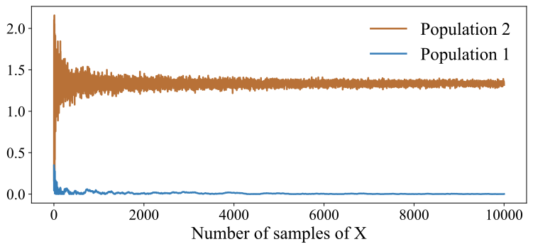
Example 2 (Myopic distribution).
Consider a like in example 1. Here, it is clear that . Consider, then, such that:
To test whether is myopic, we employed a simple test utilizing a statistical distance ( with the identity kernel) between and . This way, if , it would be clear that the equality holds. As a control measure, we also calculated the same distance for a different population , where . We have plotted the results in image 6, where Population 1 refers to and Population 2 to . As we can see, we do obtain a positive result in the test of myopicity for and a negative one for .
A.4 GSAAL (extension)
We now extend the results from section 3.2 by providing the pseudocode for the training of our method. It is important to consider that, while theorem 3 formulates the optimization problem in terms of the neural networks and , in practice this will not be the case. Instead, we will consider the optimization in terms of their weights, and . Therefore, in practice, the convergence into an equilibrium will be limited by the capacity of the networks themselves Goodfellow et al. (2016). We considered the optimization to follow minibatch-stochastic gradient descent Goodfellow et al. (2016). To consider any other minibatch-gradient method it will suffice to perform the necessary transformations to the gradients.
The pseudocode is located in Algorithm 1. As it is the training for the method, it takes both the parameters for the method and the training. In this case, refers to the total number of epochs we will train in total, while marks the epoch where we start step 2 of the GAAL training. Lines 1-3 initialize both the detectors in their subspaces and the generator with random weight matrices and . Lines 4-13 correspond to the normal GAN training loop across multiple epochs, which we referred to as step 1 of a GAAL method in the main text, if . Here we proceed with training each detector and the generator using their gradients. Lines 8-10 update each detector by ascending its stochastic gradient, while line 11 updates the generator by descending its stochastic gradient. After the normal GAN training, we start the active learning loop Liu et al. (2020) once . The only difference with the regular GAN training is that remains fixed, i.e., we do not descend using its gradient. This allows us to additionally train the detectors and, in case of equilibrium of step 1, converge to the desired marginal distributions as derived in theorem 3.
Appendix B Experimental Appendix
In this section, we will include a supplementary experiment testing the IA condition for competition, and an extension of both experimental studies featured in the main text. All of the code for the extra experiment, as well as for all experiments in the main text, can be found in our remote repository333https://github.com/WamboDNS/GSAAL.
B.1 Effects of Inlier Assumptions on Outlier Detection
| Outlier Type | Assumption Description | Outlier Description | |||||
|---|---|---|---|---|---|---|---|
| Local |
|
|
LOF | ||||
| Angle |
|
|
ABOD | ||||
| Cluster |
|
|
GAAL methodologies are capable of dealing with the inlier assumption by learning the correct inlier distribution without any assumption Liu et al. (2020). While this should also extend to our methodology, we will study experimentally whether this condition holds in practice. To do so, as one cannot identify beforehand whether a method is going to fail due to IA, we will generate synthetic datasets. This will allow us to generate outliers that we know to follow from a specific IA, ensuring that failure comes from the anomalies themselves. We will include all of the code in the code repository. To generate the synthetic datasets we follow:
-
1.
Generate , a population of inliers following some distribution in .
-
2.
Select an outlier detection method with some assumption about the normality of the data and fit it using . We will call such as the reference model for the generation.
-
3.
Generate outliers by sampling on uniformly and keeping only those points such that (i.e., they are detected as outliers). We will write to refer to such a collection of points.
-
4.
Repeat step 3 times, to obtain .
-
5.
Sample out of the points in . The remainder will be stored in , and the other in together with each .
These steps were repeated times with different , to create different training sets and different testing sets, corresponding to a total of different datasets employed per model selected in step 2. As we used different reference models, we have a total of different datasets employed in this experiment alone. In particular, the models used for this are collected in table 5. The table contains the name of the outlier type, the description of the IA taken to generate them, and a brief description of how the outliers should look. Column contains the method employed to generate each, these being , , and the same inlier distribution as , but with multiple shifted means and with a significantly lower amount of points . A visualization of how these outliers would look with features is located in figure 7.
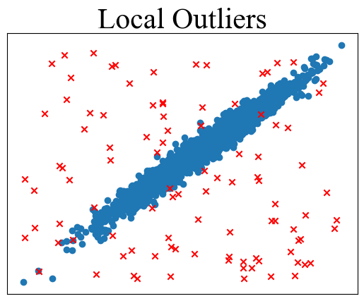
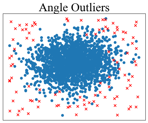
To study how different methods behave when detecting these outliers, we have performed the same experiments as in section 4.3, but with these synthetic datasets. Figure 8 gathers all the AUCs of a method in boxplots, one for each outlier type in each training set. Additionally, we grouped all based on the IA and assigned a similar color for all of them. We have done this for the classical OD methods LOF, ABOD, and kNN, besides our method GSAAL. We cropped the image below in the axis as we are not interested in results below a random classifier. As we can see, classical methods seem to correctly detect outliers for an outlier type that verifies its IA. However, whenever we introduce outliers behaving outside of their IA, the performance hit is significant. Notoriously, it appears that none of them had trouble detecting the Local and Angle outlier type. regardless of their IA. This can be easily explained by those outliers types being similar, as we can see in figure 7. On the other hand, GSAAL manages to have a significant detection rate regardless of the outlier type.
B.2 Effects of Multiple Views on Outlier Detection (extension)
In this section, we will include a brief description of the generation process for the datasets used in section 4.2. We will also perform the same experiment as in section 4.2 for all methods showcased in the main text and additional datasets. The datasets were generated by the following formulas:
-
•
Banana. Given we have and .
-
•
Spiral. Given and , we have and .
-
•
Star. Given and we have and .
-
•
Circle. Given , we have and
-
•
L. Given ; we have and
We considered to denote a random normal realization with and , and to denote a uniform realization in the interval.
Figure 9 contains all images from the MV experiment. We do not have any new insight beyond the ones exposed in the main article. Note that we have included all methods but SOD. The reason was that SOD failed to execute for datasets Star, Spiral, and Circle.
B.3 One-class Classification (extension)
As we noted in Section 4, we obtained our benchmark datasets from Han et al. (2022), a benchmark study for One-class classification methods in tabular data. Some of the datasets featured in the study, and also in our experiments, were obtained from embedding image or text data using a pre-trained NN (ResNet He et al. (2015) and BERT Devlin et al. (2019), respectively). We refrain the interested reader into Han et al. (2022) for additional information. Additionally, we found discrepancies between the versions of the datasets in the study of Campos et al. (2016) and Han et al. (2022). We utilized the version of those datasets featured in Campos et al. (2016) for our experiments due to popularity. This affected the datasets Arrhythmia, Annthyroid, Cardiotocography, InternetAds, Ionosphere, SpamBase, Waveform, WPBC and Hepatitis.
Table 6 contains all of the AUCs from our experiments. We have included extra methods that, although popular and readily available, were either too similar to other methods in our related work that were more popular (Deep SVDD and INNE) or too far away from our related work (AnoGAN) to be included in the main text. Nevertheless, due to their popularity and inclusion in the libraries used to perform the experiments, we include their results in the appendix for further comparison. Particularly, for INNE we utilized their implementation and default hyperparameters from pyod for the experiments. For DeepSVDD Ruff et al. (2018) and AnoGAN Schlegl et al. (2017), as there are no official guides on how to fit the models, we tried different training parameter combinations and took the highest obtained AUC. We used their implementation in their official code repository. Whenever a method failed to execute in a particular dataset we denoted it as FA. As it is standard in these studies Campos et al. (2016); Liu et al. (2020), we did not use those datasets subsequent statistical tests.
| Dataset | GSAAL | LOF | IForest | ABOD | SOD | KNN | SVDD | MO-GAAL | GMM | DeepSVDD | AnoGAN | INNE |
|---|---|---|---|---|---|---|---|---|---|---|---|---|
| annthyroid | 0,7681 | 0,6753 | 0,7094 | 0,7008 | 0,5243 | 0,6291 | 0,4611 | 0,5047 | 0,6932 | 0,872 | 0,4038 | 0,5081 |
| Arrhythmia | 0,7532 | 0,7277 | 0,7695 | 0,7422 | 0,6514 | 0,7334 | 0,7442 | 0,6901 | 0,7296 | 0,7485 | 0,6133 | 0,7471 |
| Cardiotocography | 0,8727 | 0,8038 | 0,7772 | 0,7956 | 0,3524 | 0,7733 | 0,8351 | 0,7912 | 0,7413 | 0,874 | 0,3248 | 0,8024 |
| CIFAR10 | 0,7862 | 0,7333 | 0,6853 | 0,7622 | 0,6607 | 0,7493 | 0,7074 | 0,6256 | 0,7462 | 0,6158 | 0,3705 | 0,7306 |
| FashionMNIST | 0,8001 | 0,8995 | 0,8298 | 0,9009 | 0,7136 | 0,9179 | 0,8130 | 0,7930 | 0,9072 | 0,6981 | 0,7137 | 0,8953 |
| fault | 0,6726 | 0,6436 | 0,6518 | 0,8019 | 0,5670 | 0,7849 | 0,5651 | 0,6821 | 0,6856 | 0,4972 | 0,4074 | 0,6026 |
| InternetAds | 0,7809 | 0,8565 | 0,4739 | 0,8600 | 0,3663 | 0,8090 | 0,7063 | 0,7603 | 0,9113 | 0,8411 | 0,5165 | 0,7643 |
| Ionosphere | 0,9593 | 0,9591 | 0,9377 | 0,9483 | 0,8250 | 0,9825 | 0,8379 | 0,9727 | 0,9644 | 0,967 | 0,8406 | 0,9596 |
| landsat | 0,5217 | 0,7598 | 0,5927 | 0,7627 | 0,4821 | 0,7726 | 0,4792 | 0,4432 | 0,4998 | 0,69 | 0,4835 | 0,6672 |
| letter | 0,6625 | 0,8888 | 0,6493 | FA | 0,7182 | 0,9066 | 0,9334 | 0,4828 | 0,8435 | 0,676 | 0,5257 | 0,7224 |
| mnist | 0,7638 | 0,9484 | 0,8647 | 0,9189 | 0,4858 | 0,9318 | FA | 0,6151 | 0,9210 | 0,7604 | 0,2502 | 0,8980 |
| optdigits | 0,8935 | 0,9991 | 0,8625 | 0,9846 | 0,4260 | 0,9983 | 0,9999 | 0,8105 | 0,8221 | 0,9086 | 0,6203 | 0,9012 |
| satellite | 0,8630 | 0,8456 | 0,7834 | FA | 0,4745 | 0,8753 | 0,8740 | FA | 0,7957 | 0,7798 | 0,3099 | 0,8309 |
| satimage-2 | 0,9836 | 0,9966 | 0,9910 | 0,9977 | 0,6745 | 0,9992 | 0,9826 | 0,6317 | 0,9967 | 0,9755 | 0,3968 | 0,9984 |
| SpamBase | 0,8717 | 0,7132 | 0,8374 | 0,7730 | 0,3774 | 0,7036 | 0,6302 | 0,7377 | 0,8034 | 0,7807 | 0,4826 | 0,6653 |
| speech | 0,6029 | 0,5075 | 0,5030 | 0,8741 | 0,4364 | 0,4853 | 0,4640 | 0,5138 | 0,5217 | 0,6076 | 0,4821 | 0,4800 |
| SVHN | 0,6859 | 0,7192 | 0,5834 | 0,6989 | 0,5781 | 0,6788 | 0,6150 | 0,7055 | 0,6684 | 0,5894 | 0,4621 | 0,6488 |
| Waveform | 0,8092 | 0,7530 | 0,6902 | 0,7115 | 0,5814 | 0,7623 | 0,5514 | 0,6049 | 0,5791 | 0,7214 | 0,7018 | 0,7562 |
| WPBC | 0,6326 | 0,5695 | 0,5681 | 0,6156 | 0,5333 | 0,5830 | 0,5681 | 0,5972 | 0,5660 | 0,4907 | 0,4121 | 0,5738 |
| Hepatitis | 0,6982 | 0,5030 | 0,6568 | 0,5207 | 0,2959 | 0,5680 | 0,4024 | FA | 0,7574 | 0,8284 | 0,3787 | 0,5325 |
| MVTec-AD | 0,9806 | 0,9679 | 0,9755 | 0,9689 | 0,9662 | 0,9703 | 0,9645 | 0,6412 | 0,9776 | 0,7422 | 0,5179 | 0,9720 |
| 20newsgroups | 0,5535 | 0,7854 | 0,6675 | FA | 0,7109 | 0,7260 | 0,6329 | 0,5313 | 0,8103 | 0,6063 | 0,4833 | 0,7074 |
References
- Aggarwal [2017] Charu C. Aggarwal. Outlier Analysis. Springer International Publishing, Cham, 2017.
- Bellman [1957] Richard Bellman. Dynamic programming. Princeton, New Jersey: Princeton University Press. XXV, 342 p. (1957)., 1957.
- Breunig et al. [2000] Markus M. Breunig, Hans-Peter Kriegel, Raymond T. Ng, and Jörg Sander. LOF: identifying density-based local outliers. In SIGMOD Conference, pages 93–104. ACM, 2000.
- Campos et al. [2016] Guilherme O. Campos, Arthur Zimek, Jörg Sander, Ricardo J. G. B. Campello, Barbora Micenková, Erich Schubert, Ira Assent, and Michael E. Houle. On the evaluation of unsupervised outlier detection: measures, datasets, and an empirical study. Data Mining and Knowledge Discovery, 30(4):891–927, Jul 2016.
- Choi and Han [2022] Jinyoung Choi and Bohyung Han. Mcl-gan: Generative adversarial networks with multiple specialized discriminators. In S. Koyejo, S. Mohamed, A. Agarwal, D. Belgrave, K. Cho, and A. Oh, editors, Advances in Neural Information Processing Systems, volume 35, pages 29597–29609. Curran Associates, Inc., 2022.
- Chollet and others [2015] François Chollet et al. Keras. https://keras.io, 2015.
- Conover and Iman [1979] W Conover and R Iman. Multiple-comparisons procedures. informal report. Technical report, Los Alamos National Laboratory (LANL), February 1979.
- Conover [1999] W. J. (William Jay) Conover. Practical nonparametric statistics / W.J. Conover. Wiley series in probability and statistics. Applied probability and statistics section. Wiley, New York ;, third edition. edition, 1999.
- Devlin et al. [2019] Jacob Devlin, Ming-Wei Chang, Kenton Lee, and Kristina Toutanova. Bert: Pre-training of deep bidirectional transformers for language understanding. In North American Chapter of the Association for Computational Linguistics, 2019.
- Donahue et al. [2017] Jeff Donahue, Philipp Krähenbühl, and Trevor Darrell. Adversarial feature learning. In International Conference on Learning Representations, 2017.
- Durugkar et al. [2016] Ishan Durugkar, Ian M. Gemp, and Sridhar Mahadevan. Generative multi-adversarial networks. ArXiv, abs/1611.01673, 2016.
- Désir et al. [2013] Chesner Désir, Simon Bernard, Caroline Petitjean, and Laurent Heutte. One class random forests. Pattern Recognition, 46(12):3490–3506, 2013.
- El-Yaniv and Nisenson [2006] Ran El-Yaniv and Mordechai Nisenson. Optimal single-class classification strategies. In B. Schölkopf, J. Platt, and T. Hoffman, editors, Advances in Neural Information Processing Systems, volume 19. MIT Press, 2006.
- Goodfellow et al. [2014] Ian Goodfellow, Jean Pouget-Abadie, Mehdi Mirza, Bing Xu, David Warde-Farley, Sherjil Ozair, Aaron Courville, and Yoshua Bengio. Generative adversarial nets. In Z. Ghahramani, M. Welling, C. Cortes, N. Lawrence, and K.Q. Weinberger, editors, Advances in Neural Information Processing Systems, volume 27. Curran Associates, Inc., 2014.
- Goodfellow et al. [2016] Ian Goodfellow, Yoshua Bengio, and Aaron Courville. Deep Learning. MIT Press, 2016. http://www.deeplearningbook.org.
- Guo et al. [2021] Jifeng Guo, Zhiqi Pang, Miaoyuan Bai, Peijiao Xie, and Yu Chen. Dual generative adversarial active learning. Applied Intelligence, 51(8):5953–5964, Aug 2021.
- Gupta et al. [2017] Nikhil Gupta, Dhivya Eswaran, Neil Shah, Leman Akoglu, and Christos Faloutsos. Lookout on time-evolving graphs: Succinctly explaining anomalies from any detector, 2017.
- Han et al. [2022] Songqiao Han, Xiyang Hu, Hailiang Huang, Minqi Jiang, and Yue Zhao. Adbench: Anomaly detection benchmark. In S. Koyejo, S. Mohamed, A. Agarwal, D. Belgrave, K. Cho, and A. Oh, editors, Advances in Neural Information Processing Systems, volume 35, pages 32142–32159. Curran Associates, Inc., 2022.
- He et al. [2015] Kaiming He, X. Zhang, Shaoqing Ren, and Jian Sun. Deep residual learning for image recognition. 2016 IEEE Conference on Computer Vision and Pattern Recognition (CVPR), pages 770–778, 2015.
- Hempstalk et al. [2008] Kathryn Hempstalk, Eibe Frank, and Ian H. Witten. One-class classification by combining density and class probability estimation. In Walter Daelemans, Bart Goethals, and Katharina Morik, editors, Machine Learning and Knowledge Discovery in Databases, pages 505–519, Berlin, Heidelberg, 2008. Springer Berlin Heidelberg.
- Keller et al. [2012] Fabian Keller, Emmanuel Muller, and Klemens Bohm. Hics: High contrast subspaces for density-based outlier ranking. In 2012 IEEE 28th International Conference on Data Engineering, pages 1037–1048, 2012.
- Keller et al. [2013] Fabian Keller, Emmanuel Müller, Andreas Wixler, and Klemens Böhm. Flexible and adaptive subspace search for outlier analysis. In Proceedings of the 22nd ACM International Conference on Information & Knowledge Management, CIKM ’13, page 1381–1390, New York, NY, USA, 2013. Association for Computing Machinery.
- Kriegel et al. [2008] Hans-Peter Kriegel, Matthias Schubert, and Arthur Zimek. Angle-based outlier detection in high-dimensional data. In KDD, pages 444–452. ACM, 2008.
- Kriegel et al. [2009] Hans-Peter Kriegel, Peer Kröger, Erich Schubert, and Arthur Zimek. Outlier detection in axis-parallel subspaces of high dimensional data. In Thanaruk Theeramunkong, Boonserm Kijsirikul, Nick Cercone, and Tu-Bao Ho, editors, Advances in Knowledge Discovery and Data Mining, pages 831–838, Berlin, Heidelberg, 2009. Springer Berlin Heidelberg.
- Kruskal [1952] William H. Kruskal. A nonparametric test for the several sample problem. The Annals of Mathematical Statistics, 23(4):525–540, 1952.
- Li et al. [2017] Chun-Liang Li, Wei-Cheng Chang, Yu Cheng, Yiming Yang, and Barnabas Poczos. Mmd gan: Towards deeper understanding of moment matching network. In I. Guyon, U. Von Luxburg, S. Bengio, H. Wallach, R. Fergus, S. Vishwanathan, and R. Garnett, editors, Advances in Neural Information Processing Systems, volume 30. Curran Associates, Inc., 2017.
- Liu et al. [2008] Fei Tony Liu, Kai Ming Ting, and Zhi-Hua Zhou. Isolation forest. In 2008 Eighth IEEE International Conference on Data Mining, pages 413–422, 2008.
- Liu et al. [2020] Yezheng Liu, Zhe Li, Chong Zhou, Yuanchun Jiang, Jianshan Sun, Meng Wang, and Xiangnan He. Generative adversarial active learning for unsupervised outlier detection. IEEE Transactions on Knowledge and Data Engineering, 32(8):1517–1528, 2020.
- Müller et al. [2012] Emmanuel Müller, Ira Assent, Patricia Iglesias, Yvonne Mülle, and Klemens Böhm. Outlier ranking via subspace analysis in multiple views of the data. In 2012 IEEE 12th International Conference on Data Mining, pages 529–538, 2012.
- Poggio et al. [2020] Tomaso Poggio, Andrzej Banburski, and Qianli Liao. Theoretical issues in deep networks. Proceedings of the National Academy of Sciences, 117(48):30039–30045, 2020.
- Ramaswamy et al. [2000] Sridhar Ramaswamy, Rajeev Rastogi, and Kyuseok Shim. Efficient algorithms for mining outliers from large data sets. In Proceedings of the 2000 ACM SIGMOD International Conference on Management of Data, SIGMOD ’00, page 427–438, New York, NY, USA, 2000. Association for Computing Machinery.
- Ruff et al. [2018] Lukas Ruff, Robert Vandermeulen, Nico Goernitz, Lucas Deecke, Shoaib Ahmed Siddiqui, Alexander Binder, Emmanuel Müller, and Marius Kloft. Deep one-class classification. In Jennifer Dy and Andreas Krause, editors, Proceedings of the 35th International Conference on Machine Learning, volume 80 of Proceedings of Machine Learning Research, pages 4393–4402. PMLR, 10–15 Jul 2018.
- Schlegl et al. [2017] Thomas Schlegl, Philipp Seeböck, Sebastian M. Waldstein, Ursula Schmidt-Erfurth, and Georg Langs. Unsupervised anomaly detection with generative adversarial networks to guide marker discovery. In Marc Niethammer, Martin Styner, Stephen Aylward, Hongtu Zhu, Ipek Oguz, Pew-Thian Yap, and Dinggang Shen, editors, Information Processing in Medical Imaging, pages 146–157, Cham, 2017. Springer International Publishing.
- Seliya et al. [2021] Naeem Seliya, Azadeh Abdollah Zadeh, and Taghi M. Khoshgoftaar. A literature review on one-class classification and its potential applications in big data. Journal of Big Data, 8(1):122, Sep 2021.
- Settles [2009] Burr Settles. Active learning literature survey. 2009.
- Sinha et al. [2019] Samarth Sinha, Sayna Ebrahimi, and Trevor Darrell. Variational adversarial active learning. In Proceedings of the IEEE/CVF International Conference on Computer Vision, pages 5972–5981, 2019.
- Steinbuss and Böhm [2017] Georg Steinbuss and Klemens Böhm. Hiding outliers in high-dimensional data spaces. International Journal of Data Science and Analytics, 4(3):173–189, Nov 2017.
- Wang et al. [2019] Hongzhi Wang, Mohamed Jaward Bah, and Mohamed Hammad. Progress in outlier detection techniques: A survey. IEEE Access, 7:107964–108000, 2019.
- Zhao et al. [2019] Yue Zhao, Zain Nasrullah, and Zheng Li. Pyod: A python toolbox for scalable outlier detection. Journal of Machine Learning Research, 20(96):1–7, 2019.
- Zhu and Bento [2017] Jia-Jie Zhu and José Bento. Generative adversarial active learning. arXiv preprint arXiv:1702.07956, 2017.