A direct method of continuous unwrapping the phase from an interferogram image
Abstract
A new method recovers phase difference of interfering wavefronts from a pattern of interference fringes, avoiding discontinuity problem. The continuous phase is a solution of the first order differential equation of the interferogram function computed from the fringe intensity profile selected along the pathway over the interferogram.
Unwrapping the phase from an interferogram is a common process needed for interpretion of the object wavefront shape [1]. In general, the interferogram could be treated as a function with a phase as an argument. Obtaining the phase from the interferogram function requires solving a trigonometric equation by inversion [1], outputting the phase in the so-called wrapped form. The wrapped phase is periodic function exhibiting a type of discontinuity and spatially aligned with the interference fringes on the interferogram. The process of unwrapping, i.e., making the countinuous phase from the pieces is challenging due to this discontinuity, because it requires to track where on the interferogram the pieces of the phase must be shifted by . The current state of solving the discontinuity problem is based on the automatic algorithmic approach and require to recognising, identifying and indexing the phase pieces over the interferogram and then manipulating them to remove each individual discontinuity, thereby obtaining the absolute phase function. A number of such methods for piecewise phase unwrapping (PPU) are known and could be found elsewhere [2, 3, 4].
However, it is possible to find a different mathematical treatment, bypass the trigonomentric approach, solve the phase unwrapping task and obtain the continuous phase directly from the interferogram. This formulation eliminates the discontinuity problem, giving access to operate with the phase as a whole piece in its absolute and continuous form. Below we present the new method of continuous phase unwrapping (CPU) and give an example comparing both approaches.
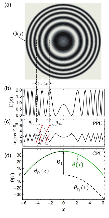
Definitions. An interferogram is defined as an image containing a pattern of bright (constructive) and dark (destructive) fringes projected from the interfering space to the image plane; see an example in Fig.1a. The fringe pattern is characterized by the grey values of the image pixels oscillating between minimal (black) and maximal (white) pixel intensities over the chosen path of the interferogram image, Fig.1b. The function contains the information of the phase difference of the interfering wavefronts of the beams. When a wavefront of the first beam is fixed (used as a reference), the whole phase difference is attributed to the wavefront of the second beam (called the object beam). The object beam, in this case, is treated as a probe to measure or characterize the properties of physical objects: topography of reflecting surfaces, shapes of lenses, thickness of thin transparent films, and so on.
The phase difference , the optical path difference (OPD) of the object wavefront with respect to the referenced one, and the wavelength satisfy a relationship
| (1) |
If the phase difference is recovered from the grey function , then Eq.(1) delivers the OPD function for given . OPD characterises the above-mentioned physical properties of the interference object once the refraction coefficients of the media where the wavefronts propagate are known.
Following [2] assume a general form of the function suitable for the interference experiment with a single pass of the object beam producing the interference fringes of infinite width
| (2) |
where the grey function , the coefficients , and the phase are the functions of a particular point on the interferogram. While oscillates in space, the coefficients are slowly varying functions of spatial coordinates [2]. Depending on the experimental conditions the coefficients represent a background illumination and an amplitude of the recorded light modulation, respectively. For simplicity we consider one-dimensional (1D) functions and .
PPU method example. The PPU approach for unwrapping from provides a discontinuous form of because being an argument of the cosine function is obtained directly from Eq.(2) [5]
| (3) |
Eq.(3) delivers the piecewise form of the phase , where each phase piece is defined within the interval corresponding to two adjacent white and black fringes (and vice versa); see an example in Fig.1c. Eq.(3) results in the oscillating or wrapped form of which must be unwrapped, providing a continuous form of which has a physically meaningful shape. The process of unwrapping for the example in Fig.1c requires identification of the types of the pieces monotonous function [5]. Then, select one type (say with odd indices, , in Fig.1c) as “true” and convert the opposite type pieces (with even indices , in Fig.1c) into the “true” type by reflecting them as shown in Fig.1c. Then shift the converted pieces with respect the preceding ones and obtain the joined pieces and corresponding now to discontinuity interval and representing only the “true” type of phase change. The continuous shape of the profile would be the result of sequentially shifting all “true” pairs by with respect to the preceding “true” pairs. All the above requires application of the appropriate pattern recognition and analysis methods to the wrapped phase, allowing recognition and indexing the fringes, splitting into pieces, converting, shifting, and then obtaining the continuous form of the unwrapped phase by manipulating the adjacent pairs. The current PPU methods are much more sophisticated than the above, but they are all designed to remove discontinuities in a piecewise manner.
CPU method. Consider an arbitrary 2D interferogram characterized by a digital grey function known for each pixel of the entire area of the interferogram. Select a straight pathway parallel to the -axis to obtain a 1D grey function of interest defined over the interval . Introduce an interferogram function – a relationship between the phase difference and the grey function obtained from a particular experimental setup. Rewrite Eq.(2) to obtain corresponding to a single passage of the object beam through the interfering medium with a unit refraction index
| (4) |
Differentiating Eq.(4) with respect to we find
| (5) |
Use Eqs.(4,5) in Pythagorean identity to eliminate the trigonometric functions from consideration and obtain
| (6) |
Note that in the differential equation Eq.(6) the phase difference is already unwrapped, i.e., is defined over the entire interval . Applying the relations , where denotes a modulus, and , where stands for the sign function returning , write the solution of Eq.(6) as
| (7) |
The function and its derivative can be obtained from Eq.(4) by employing the interference pattern . The integrand in Eq.(7) at some points in the integration interval represents the 0/0 indeterminate, however the computation shows that terms contributing to a (possible) divergence cancel out. The function could be obtained once the extremum points of are found from the equation . As at these points both sides of Eq.(6) vanish, the equation for the extrema reads
| (8) |
In general case Eq.(8) can be solved numerically. For a sequence of roots , of Eq.(8) the whole interval should be divided into a sequence of segments where each segment is characterized by a specific value of with . The sign alternates between adjacent segments. Thus, the whole sign sequence is determined by the in the first segment and it does not affect the shape of the unwrapped phase. The integral of Eq.(7) must be applied for each individual segment taking into account the phase of the preceding segment.
CPU method example. To illustrate the CPU method consider the phase difference defined as a one dimensional even parabolic function , in the interval with constant . Use Eq.(2) to obtain the grey function
| (9) |
where are constants. The goal is to evaluate Eq.(7) and find the phase . For the interferogram function is given by
| (10) |
leading to . Eq.(8) gives an equation for the roots . In the interval there is a single root , being an extremum point of the phase function, so it produces only two sign segments. In the first segment the sign , the integrand of Eq.(7) is , and the phase for this interval reads
| (11) |
where denotes the phase per segment. The phase shift for the whole first segment . For the second segment we have , the integrand is , and the phase for this interval evaluates to
| (12) |
Uniting the intervals we obtain the final phase in the entire interval reproducing the identity of the input and recovered phase, see Fig.1d.
The proposed method can be applied for defined numerically (as an array), an unknown phase may include more than one extreme point. In this case, the roots of Eq.(8) and the integral Eq.(7) are computed numerically, once the process of digitizing the experimental interference pattern provides a sufficient number of points per the narrowest fringe in the function used as an input for the interferogram function . Note, this method allows us to obtain the phase profile from the experimental profile with the accuracy of the first segment . The sign for the segment is set arbitrarily, then one obtains two profiles of the same shape but mirror reflected to each other with respect to the -axis. One might choose the correct shape by using the experimental insights usually existing for some characteristic points on the interferogram.
The presented method of continuous phase unwrapping (CPU) could be considered as complimentary to the existing one – piecewise phase unwrapping (PPU). Regarding the fundamental difference between the methods, the CPU method uses the numerical calculus approach providing access to the whole phase function without discontinuities, while PPU applies automatic algorithmic manipulations to the phase pieces to remove these discontinuities. The CPU approach may offer a new perspective in developing the methods for interferogram analysis. For example, the CPU method allows one to obtain the phase and OPD profiles [6] without the extensive programming required for the PPU method.
References
- [1] M. Georges, Holographic Interferometry: From History to Modern Applications, in Optical Holography: Materials, Theory and Applications, edited by P.-A. Blanche (Elsevier, 2019), 1st ed. pp. 121–163.
- [2] T. R. Judge and P. J. Bryanston-Cross, A Review of Phase Unwrapping Techniques in Fringe Analysis, Opt. Lasers Eng. 21, 199 (1994).
- [3] G. T. Reid, Automatic Fringe Pattern Analysis : A Review, Opt. Lasers Eng. 7, 37 (1986).
- [4] D. Malacara, M. Servín and Z. Malacara, Interferogram Analysis For Optical Testing (CRC Press, 2005), 2nd ed.
- [5] K. Okada, E. Yokoyama, and H. Miike, Interference Fringe Pattern Analysis Using Inverse Cosine Function, Denshi Joho Tsushin Gakkai Ronbunshi J86-D-II 1420 (2003), [Electron. Commun. Japan, Part 2 90, 61 (2007)].
- [6] V. Berejnov and D. Li, A Simple Method of Measuring Profiles of Thin Liquid Films for Microfluidics Experiments by Means of Interference Reflection Microscopy, arXiv:1006.2180 [physics.optics] (2010).