KATO: Knowledge Alignment And Transfer for Transistor Sizing Of Different Design and Technology

Abstract.

Automatic transistor sizing in circuit design continues to be a formidable challenge. Despite that Bayesian optimization (BO) has achieved significant success, it is circuit-specific, limiting the accumulation and transfer of design knowledge for broader applications. This paper proposes (1) efficient automatic kernel construction, (2) the first transfer learning across different circuits and technology nodes for BO, and (3) a selective transfer learning scheme to ensure only useful knowledge is utilized. These three novel components are integrated into BO with Multi-objective Acquisition Ensemble (MACE) to form Knowledge Alignment and Transfer Optimization (KATO) to deliver state-of-the-art performance: up to 2x simulation reduction and 1.2x design improvement over the baselines.

1. Introduction

The ongoing miniaturization of circuit devices within integrated circuits (ICs) introduces increasing complexity to the design process, primarily due to the amplified impact of parasitics that cannot be overlooked. In contrast to digital circuit design, where the use of standardized cells and electronic design automation (EDA) tools streamlines the process, analog and mixed-signal (AMS) designs still predominantly rely on the nuanced expertise of designers (Elfadel et al., 2019). This reliance on analog design experts is not only costly but also introduces the risk of inconsistency and bias. Such challenges can lead to inadequate exploration of the design space and extended design times. As a consequence, it often results in sub-optimal design in terms of power, performance, and area (PPA), underscoring the need for more efficient and objective design methodologies.

Analog circuit design involves two main steps: designing the circuit topology and sizing the transistors, where the former is normally guided by expert knowledge and the latter is labor-intensive and time-consuming. Thus, the transistor sizing is normally solved by algorithms to allow designers to dedicate their expertise more effectively toward the nuanced aspects of topology selection.

Machine learning advancements have heightened interest in the application of reinforcement learning (RL) to transistor sizing. Specifically, RL agents are trained to optimize the transistor sizing process by rewarding the agent with better designs that deliver higher performance. Wang et al. (2020) introduce a GCN-RL circuit designer that utilizes RL to transfer knowledge efficiently across various technology nodes and topologies with a graph convolutional network (GCN) capturing circuit topology, resulting in enhanced Figures of Merit (FOM) for a range of circuits. Li et al. (2021) expand on this by incorporating a circuit attention network and a stochastic method to diminish layout effects, while Settaluri et al. (2021) utilize a multi-agent approach for sub-block tuning for a larger circuit sizing task.

While RL’s promise is clear, it has the following limitations: (1) the inherent design for complex Markov decision processes of RL makes it an overly complex solution for the relatively straightforward optimization task of transistor sizing, leading to great demand for data of designs and simulations; (2) RL’s complexity and high computational cost may be excessive for smaller teams with limited resources; and (3) the trained model might contain commercially sensitive design information that can be exploited by competitors.

Bayesian optimization (BO) stands in contrast to reinforcement learning (RL), being a tried-and-tested optimization method for intricate EDA tasks. Its popularity stems from its efficiency, stability, and the fact that it doesn’t require pretraining, making it more accessible for immediate deployment. To solve the transistor sizing challenge as a straightforward optimization problem, Lyu et al. (2018a) introduce weighted expected improvement (EI), transforming the constrained optimization of transistor sizing into a single-objective optimization task. Building upon this, Lyu et al. (2018b) presents the Multiple Acquisition Function Ensemble (MACE) to facilitate massive parallel simulation, which is essential to harness the power of cluster computing. To resolve the large-scale transistor sizing challenge, Touloupas et al. (2021) implement multiple local Gaussian Processes (GP) with GPU acceleration to significantly improve BO scalability. The choice of kernel function is pivotal in BO’s performance. As a remedy, Bai et al. (2021) propose deep kernel learning (DKL) to construct automatic GP for efficient design space exploration.

Recognizing the similarities in transistor sizing across different technology nodes, Zhang et al. (2022) utilize Gaussian Copula to correlate technology nodes with multi-objective BO, aiming to improve the search of the Pareto frontier.

Despite its notable achievements, Bayesian Optimization (BO) faces several challenges that impede its full potential in the application of transistor sizing: (1) DKL is powerful but data-intensive and demands meticulous neural network design and training; (2) Transfer Learning in BO is only possible for technology and impossible for different designs, (3) Transfer Learning in practice may degrade performance, it is unclear when to use Transfer Learning and when not to use Transfer Learning. We propose Knowledge Alignment and Transfer Optimization, KATO, to resolve these challenges simultaneously. The novelty of this work includes:

1. As far as the authors are aware, KATO is the first BO sizing method that can transfer knowledge across different circuit designs and technology nodes simultaneously.

2. To ensure a positive Transfer Learning, we propose a simple yet effective Bayesian selection strategy in the BO pipeline.

3. As an alternative to DKL, we propose a Neural kernel (Neuk), which is more powerful and stable for BO.

4. KATO is validated using practical analog designs with state-of-the-art methods on multiple experiment setups, showcasing a 2x speedup and 1.2x performance enhancement.

2. Background

2.1. Problem Definition

Transistor sizing is typically formulated as a constrained optimization problem. The goal is to maximize a specific performance while ensuring that various metrics meet predefined constraints, i.e.,

(1) $$\operatornamewithlimits{argmax}f_{0}({\bf x})\quad\text{s.t.}\quad f_{i}({\bf x})\geq C_{i},\quad\forall i\in{1,\ldots,{{N}_{c}}}.$$

Here, ${\bf x}\in\mathbb{R}^{d}$ represents the design variable, $f_{i}({\bf x})$ calculates the i-th performance metric, and $C_{i}$ denotes the required minimum value for that metric. Given the complexity of solving this constrained optimization problem, many convert it into an unconstrained optimization problem by defining a Figure of Merit (FOM) that combines the performance metrics. For instance, (Wang et al., 2020) defines

(2) $$FOM({\bf x})=\sum_{i=0}^{N_{c}}w_{i}\times\frac{min(f_{i}({\bf x}),f_{i}^{bound})-f_{i}^{min}}{f_{i}^{max}-f_{i}^{min}},$$

where $f_{i}^{bound}$ is the pre-determined limit and $f_{i}^{max}$ and $f_{i}^{min}$ are the maximum and minimum values obtained through 10,000 random samples, $w_{i}$ is $-1or1$ depending on whether the metric is to be maximized or minimized. The FOM method is less desirable due to the difficulty in setting all hyperparameters properly.

2.2. Gaussian process

Gaussian process (GP) is a common choice as a surrogate model for building the input-output mapping for complex computer code due to its flexibility and uncertainty quantification. We can approximate the black-box function $f_{0}({\bf x})$ by placing a GP prior: $f_{0}({{\bf x}})|\boldsymbol{\theta}\sim{\mathcal{GP}}(m({{\bf x}}),k({{\bf x}},{{\bf x}}^{\prime}|\boldsymbol{\theta})),$

where the mean function is normally assumed zero, i.e., $m_{0}({{\bf x}})\equiv 0$, by virtue of centering the data. The covariance function can take many forms, the most common is the automatic relevance determinant (ARD) kernel $k({{\bf x}},{{\bf x}}^{\prime}|\boldsymbol{\theta})=\theta_{0}\exp(-({{\bf x}}-{{\bf x}}^{\prime})^{T}diag(\theta_{1},\ldots,\theta_{l})({{\bf x}}-{{\bf x}}^{\prime}))$, with $\boldsymbol{\theta}$ denoting the hyperparameters. Other kernels like Rational Quadratic (RQ), Periodic (PERD), and Matern can also be used depending on the application.

For any given design variable ${{\bf x}}$, $f({{\bf x}})$ is now considered a random variable, and multiple observations $f({{\bf x}}_{i})$ form a joint Gaussian with covariance matrix ${\bf K}=[K_{ij}]$ where $K_{ij}=k({{\bf x}}_{i},{{\bf x}}_{j})$. With a consideration of the model inadequacy and numerical noise $\varepsilon\sim\mathcal{N}(0,\sigma^{2})$, the likelihood $\mathcal{L}$ is:

(3) $$\mathcal{L}=-\frac{1}{2}{{\bf y}}^{T}(\textbf{K}+\sigma^{2}{\bf I})^{-1}{{\bf y}}-\frac{1}{2}\ln|\textbf{K}+\sigma^{2}{\bf I}|-\frac{1}{2}\log(2\pi).$$

The hyperparameters $\boldsymbol{\theta}$ in kernels are estimated via maximum likelihood estimates (MLE) of $\mathcal{L}$.

Conditioning on ${\bf y}$ gives a predictor posterior $\hat{f}({\bf x})\sim\mathcal{N}(\mu({{\bf x}}),v({{\bf x}}))$

(4) $$\small\mu({{\bf x}})={{\bf k}}^{T}({{\bf x}})\left(\textbf{K}+\sigma^{2}{\bf I}\right)^{-1}{\bf y};v({{\bf x}})=k({{\bf x}},{{\bf x}})-{{\bf k}}^{T}({{\bf x}})\left(\textbf{K}+\sigma^{2}{\bf I}\right)^{-1}{{\bf k}}({{\bf x}})$$

2.3. Bayesian Optimization

To maximize $f({\bf x})$, we can optimize ${\bf x}$ by sequentially quarrying points such that each point shows an improvement $I({\bf x})=\max(\hat{f}({\bf x})-y^{\dagger},0)$, where $y^{\dagger}$ is the current optimal and $\hat{f}({\bf x})$ is the predictive posterior in Eq. (4). The possibility for ${\bf x}$ giving improvements is

(5) $$PI({\bf x})=\Phi\left({(\mu({\bf x})-y^{\dagger})}/{\sigma({\bf x})}\right),$$

which is the probability of improvement (PI). For a more informative solution, we can take the expectative improvement (EI) over the predictive posterior:

(6) $$EI({\bf x})=(\mu({\bf x})-y^{\dagger})\psi\left(u({\bf x})\right)+v({\bf x})\phi\left(u({\bf x})\right),$$

where $\psi(\cdot)$ and $\phi(\cdot)$ are the probabilistic density function (PDF) and cumulative density function (CDF) of standard normal distribution, respectively.

The candidate for the next iteration is selected by $\operatornamewithlimits{argmax}_{{\bf x}\in\mathcal{X}}EI({\bf x})$ with gradient descent methods, e.g., L-BFGS-B. Rather than looking into the expected improvement, we can approach the optimal by exploring the areas with higher uncertainty, a.k.a, upper confidence bound (UCB)

(7) $$UCB({\bf x})=\left(\mu({\bf x})+\beta v({\bf x})\right),$$

where $\beta$ controls the tradeoff between exploration and exploitation.

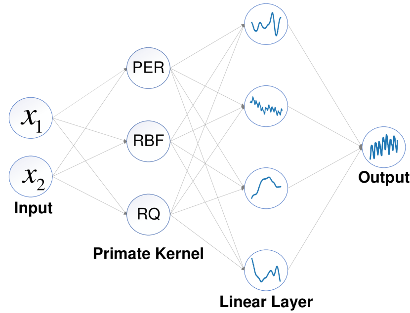
(a) Neural Kernel

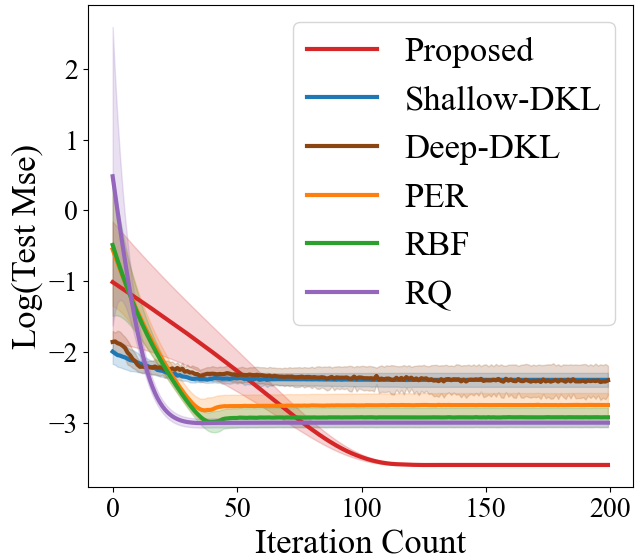
(b) Assessment

Figure 1. Neural kernel and assessments

3. Proposed methodologies

3.1. Automatic Kernel Learning: Neural Kernel

Choosing the right kernel function is vital in BO. Despite DKL’s success, creating an effective network structure remains challenging. Following (Sun et al., 2018), we introduce Neural Kernel (Neuk) as a basic unit to construct an automatic kernel function.

Neuk is inspired by the fact that kernel functions can be safely composed by adding and multiplying different kernels. This compositional flexibility is mirrored in the architecture of neural networks, specifically within the linear layers. Neuk leverages this concept by substituting traditional nonlinear activation layers with kernel functions, facilitating an automatic kernel construction.

To illustrate, consider two input vectors, ${\bf x}_{1}$ and ${\bf x}_{2}$. In Neuk, these vectors are processed through multiple kernels $\{h_{i}({\bf x},{\bf x}^{\prime})\}_{i}^{N_{k}}$, each undergoing a linear transformation as follows:

(8) $$h_{i}({\bf x}_{1},{\bf x}_{2})={h_{i}({\bf W}^{(i)}{\bf x}_{1}+{\bf b}^{(i)},{\bf W}^{(i)}{\bf x}_{2}+{\bf b}^{(i)})}$$

Here, ${\bf W}^{(i)}$ and ${\bf b}^{(i)}$ represent the weight and bias of the $i$-th kernel function, respectively, and $h_{i}(\cdot)$ is the corresponding kernel function. Subsequently, latent variables ${\bf z}$ are generated through a linear combination of these kernels:

(9) $${\bf z}={\bf W}^{(z)}{\bf h}({\bf x}_{1},{\bf x}_{2})+{\bf b}^{(z)},$$

where ${\bf W}^{(z)}$ and ${\bf b}^{(z)}$ are the weight and bias of the linear layer, and ${\bf h}({\bf x}_{1},{\bf x}_{2})=[h_{1}({\bf x}_{1},{\bf x}_{2}),\ldots,h_{d_{l}}({\bf x}_{1},{\bf x}_{2})]^{T}$. This configuration constitutes the core unit of Neuk. For broader applications, multiple Neuk units can be stacked horizontally to form a Deep Neuk (DNeuk) or vertically for a Wide Neuk (WNeuk). However, in this study, we utilize a single Neuk unit, finding it sufficiently flexible and efficient without excessively increasing the parameter count.

The final step in the Neuk process involves a nonlinear transformation applied to the latent variables ${\bf z}$, ensuring the semi-positive definiteness of the kernel function,

(10) $$k_{neuk}({\bf x}_{1},{\bf x}_{2})=\exp(\textstyle\sum z_{j}+b^{(k)}).$$

A graphical representation of the Neuk architecture is shown in Fig. 1 along with small experiments demonstrating its effectiveness in predicting performance in a 180nm second-stage amplification circuit (see Section 4) with 100 training and 50 testing data points.

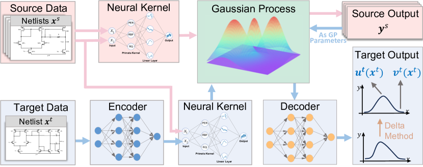
Figure 2. Knowledge Alignment and Transfer (KAT)-GP

3.2. Knowledge Alignment and Transfer

In the literature, transfer learning is predominantly based on deep learning, wherein the knowledge is encoded within the neural network weights, facilitating transfer learning through the method of fine-tuning these weights on a target dataset. Contrastingly, GPs present a fundamentally different paradigm. The predictive capability of GPs is intrinsically tied to the source data they are trained on (see Eq. (4)). This reliance on data for prediction underscores a significant challenge in applying transfer learning to GPs.

To address the challenge of applying transfer learning to GPs, we propose an innovative encoder-decoder structure, which we refer to as Knowledge Alignment and Transfer (KAT) in GPs. This approach retains the intrinsic knowledge of the source GP while aligning it with the target domain through an encoder and decoder mechanism.

Consider a source dataset $\mathcal{D}^{(s)}=\{({\bf x}^{(s)}_{i},{\bf y}^{(s)}_{i})\}$, on which the GP model $GP({\bf x})$ is trained, and a target dataset $\mathcal{D}^{(t)}=\{({\bf x}^{(t)}_{i},{\bf y}^{(t)}_{i})\}$. The first step involves introducing an encoder ${\bf E}({\bf x})$, which maps the target input ${\bf x}^{(t)}$ into the source input space ${\bf x}^{(s)}$. This encoder accounts for potential differences in dimensionality between the source and target datasets, effectively managing any compression or redundancy.

The target outputs may have different value ranges or even quantities from the source outputs. We employ a decoder ${\bf D}({\bf y}^{(s)})$ that transforms the output of the GP $G({\bf x})$ to match the target output ${\bf y}^{(t)}$. Thus, the KAT-GP for the target domain is expressed as ${\bf y}^{(s)}={\bf D}(GP({\bf E}({\bf x}^{(t)})))$.

A key aspect of this approach is that the original observations in the source GP are preserved, while the encoder and decoder are specifically trained to align and transfer knowledge between the source and target domains. The encoder and decoder themselves can be complex functions, such as deep neural networks, and their specific architecture depends on the problem and available data. In this work, both the encoder and decoder are small shallow neural networks with linear($d_{in}\times{32}$)-sigmoid-linear(${32}\times d_{out}$) structure, where $d_{in}$ and $d_{out}$ are the input and output dimension during implementation.

It is important to note that unless the decoder is a linear operator, KAT-GP is no longer a GP and does not admit a closed-form solution. We approximate the predictive mean and variance of the overall model through the Delta method, which employs Taylor series expansions to estimate the predictive mean $\boldsymbol{\mu}^{(t)}({\bf x}^{(t)})$ and covariance ${\bf S}^{(t)}({\bf x}^{(t)})$ of the transformed output:

(11) $$\mu^{(t)}({\bf x}^{(t)}) =D\left(\boldsymbol{\mu}^{(s)}(E({\bf x}^{(t)}))\right);\quad{\bf S}^{(t)}({\bf x}^{(t)}) ={\bf J}{\bf S}^{(s)}{\bf J}^{T},$$

where $\boldsymbol{\mu}^{(s)}({\bf x}^{(s)})$ and ${\bf S}^{(s)}({\bf x}^{(s)})$ are the predictive mean and covariance of $GP({\bf x})$, respectively, and ${\bf J}$ is the Jacobian matrix of ${\bf D}(\mu^{(t)}({\bf x}^{(t)}))$ with respect to $\boldsymbol{\mu}^{(t)}({\bf x}^{(t)})$. Thus, training of KAT-GP involves maximizing the log-likelihood in Eq. (12) using gradient descent w.r.t the parameters of the encoder and decoder, as well as the hyperparameters of the neural kernel.

(12) $$\mathcal{L}=\sum\log\mathcal{N}({\bf y}^{(t)}_{i}|D(\boldsymbol{\mu}(E({\bf x}^{(t)}_{i}))),{\bf J}_{i}{\bf S}_{i}{\bf J}_{i}^{T}+\sigma^{2}_{t}{\bf I},).$$

KAT-GP is illustrated in Fig. 2. It offers the first knowledge transfer solution for GP with different design and performance space.

3.3. Modified Constrained MACE

In transistor sizing, it is crucial to harness the power of parallel computing by running multiple simulations simultaneously. One of the most popular solutions, MACE (Zhang et al., 2021) resolves this challenge by proposing candidates lying on the Pareto frontier of objectives $\{{UCB}({\bf x}),{PI}({\bf x}),{EI}({\bf x}),{PF}({\bf x}),\sum_{i=1}^{N_{c}}\max(0,u_{i}({\bf x})),\sum_{i=1}^{N_{c}}\max(0,\frac{u_{i}({\bf x})}{v_{i}({\bf x})})\}$
using Genetic searching NSGA-II. Here, ${PF}({\bf x})$ is the probability of feasibility, which use Eq. (5) with all constraint metrics, i.e., ${PF}({\bf x})=\prod_{i}^{N_{c}}\Phi({u_{i}({\bf x})-C_{i}}/{v_{i}({\bf x})})$.

Despite its success, MACE suffers from high computational complexity, as it requires a Pareto front search with six correlated objectives. To mitigate this issue, we consider the constraint as an additional objective for the primal metric $f_{0}({\bf x})$ and the multi-objective optimization becomes

(13) $$\operatornamewithlimits{argmax}\{{UCB}({\bf x}),{PI}({\bf x}),{EI}({\bf x})\}\times PF({\bf x}).$$

This reduction in dimensionality significantly improves efficiency, as the complexity grows exponentially with the number of objectives while maintaining the same level of performance. Empirically, we do not observe any performance degradation.

3.4. Selective Transfer Learning with BO

While transfer learning proves effective in numerous scenarios, its utility is not universal, particularly when the source and target domains differ significantly, such as between an SRAM and an ADC. It’s important to note that even when the source and target datasets have an equal number of points, the utility of KAT-GP may not be immediately apparent. However, our empirical studies reveal that source and target data often exhibit distinctly different distributions, with varying concentration regions. This divergence can provide valuable insights for the optimization of the target circuit, even when the target data exceeds the source data in size. The effectiveness of transfer learning in such cases is inherently problem-dependent, requiring adaptable strategies for diverse scenarios.

To address these challenges, we propose a Selective Transfer Learning (STL) strategy, which synergizes with the batch nature of the MACE algorithm to optimize the benefits of transfer learning. This approach involves training both a KAT-GP model and a GP model (referred to as NeukGP, equipped with a Neural Kernel) exclusively on the target data. During the Bayesian Optimization (BO) process, each model collaborates with MACE to generate proposal Pareto front sets, denoted as $\mathcal{P}i$ (with $i=1,2$ in this context). We randomly select $\frac{w{1}}{w{1}+w_{2}}N_{B}$ points from $\mathcal{P}1$ to form $\mathcal{A}1$, and $\frac{w{2}}{w{1}+w_{2}}N_{B}$ points from $\mathcal{P}_{2}$ to form $\mathcal{A}_{2}$. Points in $\mathcal{A}1$ and $\mathcal{A}2$ are then simulated and evaluated. The weights are initialized with the number of samples and updated based on the number of simulations that improve the current best, i.e.,

(14) $$w_{i}=w_{i}+|f(\mathcal{A}i)>y^{\dagger}|_{n},$$

where $|f(\mathcal{A}i)>y^{\dagger}|_{n}$ represents the number of points in $\mathcal{A}i$ that surpass the current best objective value $y^{\dagger}$, and $f$ can be the constrained objective or the Figure of Merit (FOM). The STL algorithm is summarized in Algorithm 1.

Algorithm 1 KATO with Selective Transfer Learning

0:  Source dataset $\mathcal{D}_{s}$ , initial target circuit data $\mathcal{D}_{t}$, # iterations $N_{I}$. $B$, batch size $N_{B}$ per iteration

1:  Train KAT-GP on $\mathcal{D}_{s}$ and $\mathcal{D}_{t}$

2:  Train NeukGP based on $\mathcal{D}_{t}$

3:  for $i=1\to N_{I}$ do

4:     Update KAT-GP and NeukGP based on $\mathcal{D}_{t}$

5:     Apply MACE to KAT-GP and NeukGP to generate proposal set $\mathcal{P}_{1}$ and $\mathcal{P}_{2}$.

6:     Form action set $\mathcal{A}_{1}$ and $\mathcal{A}_{2}$ by randomly selecting $\frac{w_{1}}{w_{1}+w_{2}}N_{B}$ points from $\mathcal{P}_{1}$ and $\frac{w_{2}}{w_{1}+w_{2}}N_{B}$ points from $\mathcal{P}_{2}$.

7:     Simulate $\mathcal{A}_{1}$ and $\mathcal{A}_{2}$ and update $\mathcal{D}_{t}\leftarrow\mathcal{D}_{t}\cup\mathcal{A}_{1}\cup\mathcal{A}_{2}$.

8:     Update $w_{1}$ and $w_{2}$ based on Eq. (14) and best design ${\bf x}_{*}$.

9:  end for

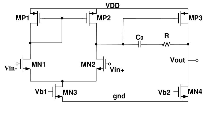
(a) Two-stage operational amplifier

(b) Three-stage operational amplifier

(c) Bandgap

Figure 3. Schematic of the evaluation circuits

4. Experiment

To assess the effectiveness of KATO, we conducted experiments on three analog circuits: a Two-stage operational amplifier (OpAmp), a Three-stage OpAmp, and a Bandgap circuit (depicted in Fig. 3).

Two-stage Operational Amplifier (OpAmp) focuses on optimizing the length of the transistors in the first stage, the capacitance of the capacitors, the resistance of the resistors, and the bias currents for both stages. The objective is to minimize the total current consumption ($I_{total}$) while meeting specific performance criteria: phase margin (PM) greater than 60 degrees, gain-bandwidth product (GBW) over 4MHz, and a gain exceeding 60dB.

(15) $$\operatornamewithlimits{argmin}I_{total};\text{s.t.};PM>60^{\circ},GBW>4MHz,Gain>60dB.$$

Three-stage OpAmp improves the gain beyond what a two-stage OpAmp can offer with an additional stage. This variant introduces more design variables, including the length of transistors in the first stage, the capacitance of two capacitors, and the bias currents for all three stages. The optimization is specified as:

(16) $$\operatornamewithlimits{argmin}I_{total};\text{s.t.};PM>60^{\circ},GBW>2MHz,Gain>80dB.$$

Bandgap Reference Circuit is vital in maintaining precise and stable outputs in analog and mixed-signal systems-on-a-chip. The design variables include the length of the input transistor, the widths of the bias transistors for the operational amplifier, and the resistance of the resistors. The aim is to minimize the temperature coefficient (TC), with constraints on total current consumption ($I_{total}$ less than 6uA) and power supply rejection ratio (PSRR larger than 50dB):

(17) $$\operatornamewithlimits{argmin}TC;\text{s.t.};I_{total}<6uA,PSRR>50dB.$$

For the experiments, each method was repeated five times with different random seeds, and statistical results were reported.

Baselines were implemented with fine-tuned hyperparameters to ensure optimal performance. All circuits were implemented using 180nm and 40nm Process Design Kits (PDK). KATO is implemented in PyTorch with MACE. Experiments were carried out on a workstation equipped with an AMD 7950x CPU and 64GB RAM.

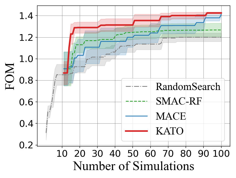
(a) Two-stage OpAmp

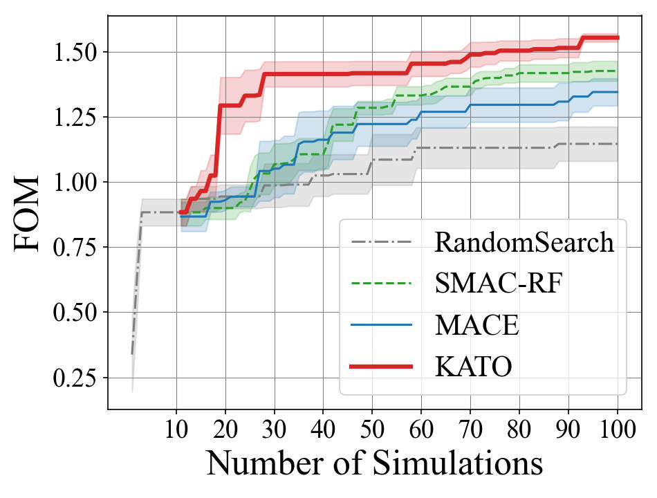
(b) Three-stage OpAmp

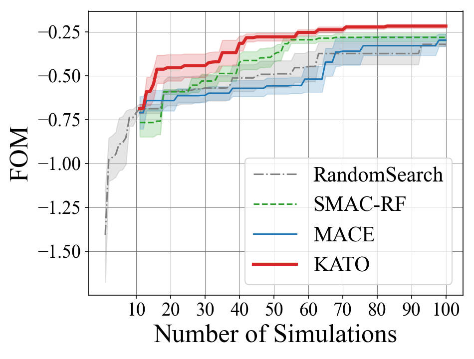
(c) Bandgap

Figure 4. Transistor sizing by optimizing FOM

4.1. Assessment of FOM Optimization

We initiated the evaluation based on the FOM of Eq. (2). KATO was compared against SOTA Bayesian Optimization (BO) techniques for a single objective, SMAC-RF, along with MACE and a naive random search (RS) strategy. All methods are given 10 random simulations as the initial dataset, and the sizing results (FOM versus simulation budget) for the 180nm technology node are shown in Fig. 4. SMAC-RF is slightly better than MACE due to this simple single-objective optimization task. Notably, KATO outperforms the baselines by a large margin. Particularly, KATO consistently achieves the maximum FOM, with up to 1.2x improvement, and it takes about 50% fewer simulations to reach a similar optimal FOM. The optimal result of RS does not actually satisfy all constraints, highlighting the limitation of FOM-based optimization.

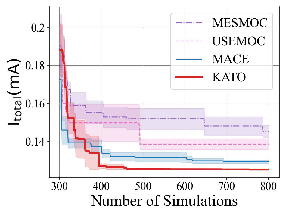
(a) Two-stage OpAmp

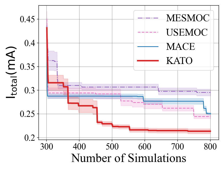
(b) Three-stage OpAmp

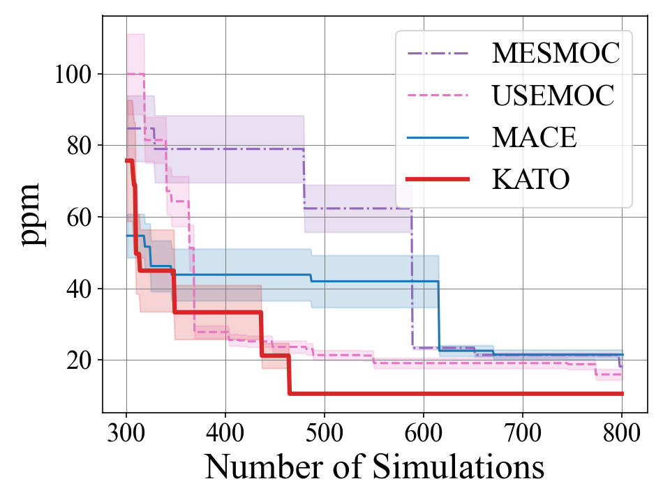
(c) Bandgap

Figure 5. Transistor sizing by constrained optimization

Table 1. Transistor Sizing Optimal Performance via Optimization with Constraints

Two-stage OpAmp(180nm) Three-stage OpAmp(180nm) Bandgap(180nm) Method I(uA) Gain(dB) PM(^∘) GBW(MHz) I(uA) Gain(dB) PM(^∘) GBW(MHz) TC(ppm/^∘C) I(uA) PSRR(dB @100Hz) Specifications min ¿60 ¿60 ¿4 min ¿80 ¿60 ¿2 min ¡6 ¿50 Human Expert 274.84 75.12 63.57 8.23 462.84 112.49 65.61 2.05 11.26 5.31 61.01 MSEMOC 138.58 80.39 65.28 5.66 288.28 86.85 73.55 2.27 14.04 5.29 60.97 USEMOC 137.89 65.42 66.63 4.63 230.47 81.24 73.67 2.09 10.36 4.78 61.21 MACE 127.69 79.30 61.50 4.38 245.62 81.02 68.38 2.13 10.41 4.78 61.20 KATO 124.21 61.18 60.59 4.56 187.51 80.3 63.99 2.10 9.66 5.42 61.99

4.2. Assessment of Constrained Optimization

Next, we assess the proposed method of transistor sizing with a more practical and challenging constrained optimization setup. During optimization, only designs satisfying all constraints are considered valid and included in the performance reports. To provide sufficient valid designs for the surrogate model, we first simulate 300 random designs, typically yielding about 7 valid designs, a 2.3% that makes RS not applicable in this task.

We compare KATO with SOTA constrained BO tailored for circuit design, namely, MESMOC (Belakaria et al., 2020a), USEMOC (Belakaria et al., 2020b), and MACE with constraints (Zhang et al., 2021). The results of 180nm are shown in Fig. 5, where MESMOC shows a poor performance due to its lack of exploration, and MACE is generally good except for the three-stage OpAmp. KATO demonstrates a consistent superiority, always achieving the best performance with a clear margin, and most importantly, with about 50% of simulation cost to reach the best-performing baseline. The final design performance is shown in Table 1, where KATO achieves the best performance by extreme trade-off for the constraints (e.g., Gain) as long as they fulfilling the requirements.

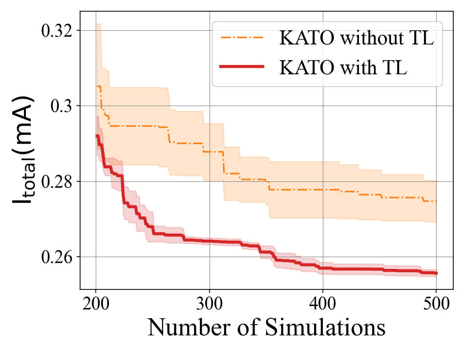
(a) Two-stage OpAmp (180nm) To Two-stage OpAmp (40nm)

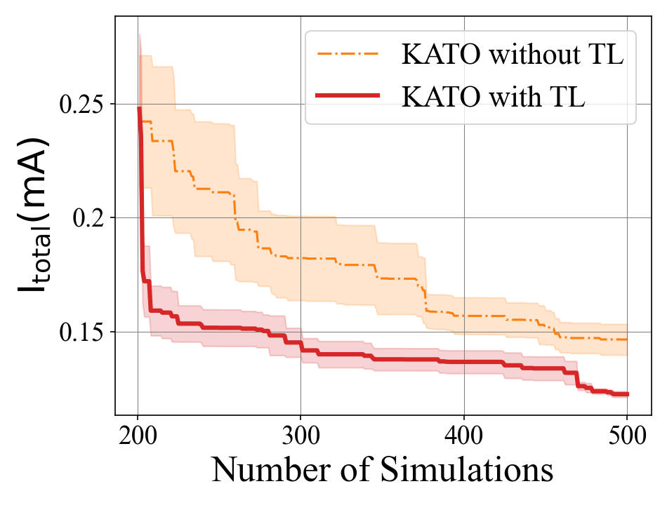
(b) Three-stage OpAmp (180nm) To Three-stage OpAmp (40nm)

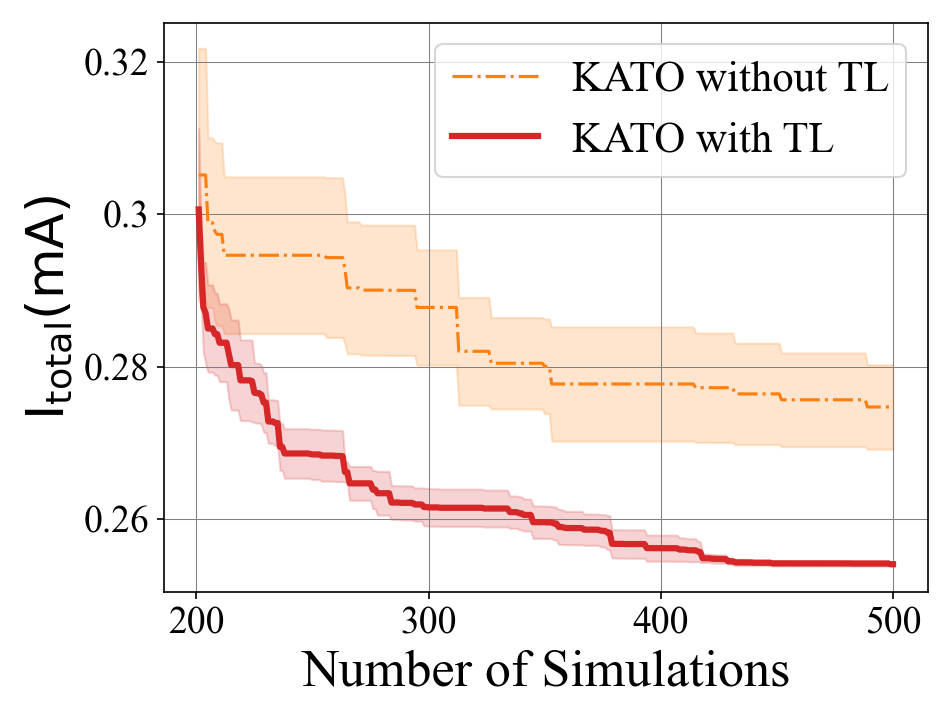
(c) Three-stage OpAmp (40nm) To Two-stage OpAmp (40nm)

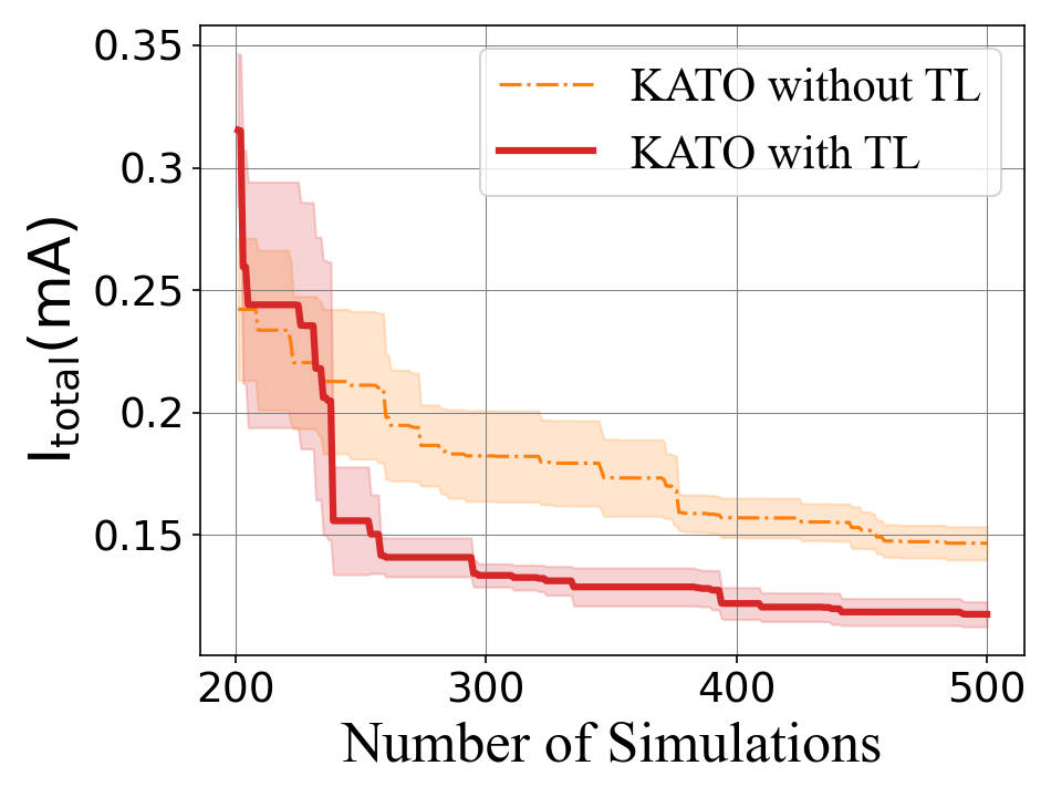
(d) Two-stage OpAmp (40nm) To Three-stage OpAmp (40nm)

(e) Three-stage OpAmp (180nm) To Two-stage OpAmp (40nm)

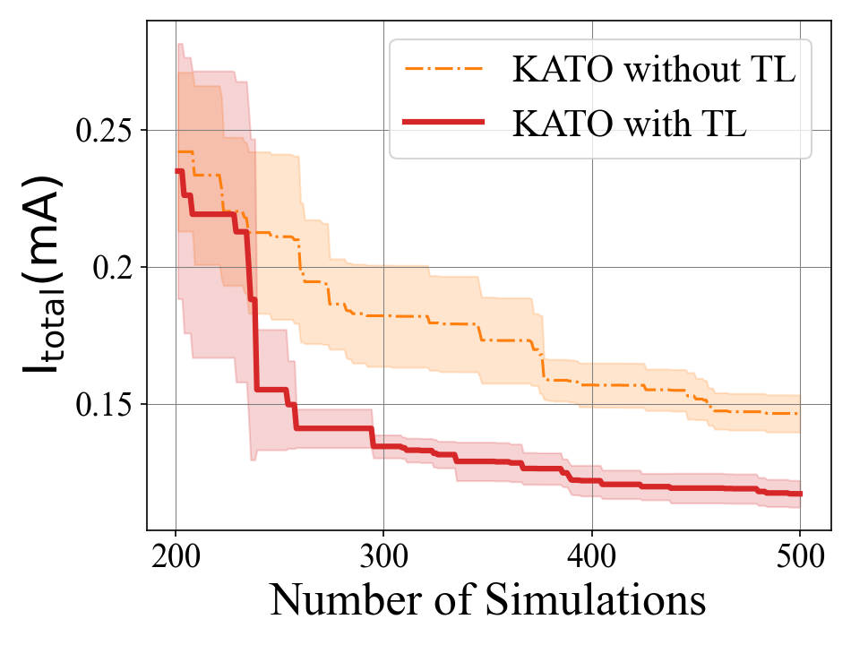
(f) Two-stage OpAmp (180nm) To Three-stage OpAmp (40nm)

Figure 6. Transistor sizing constrained optimization with Transfer Learning of designs and technology node

4.3. Assessment of Transfer Learning

Finally, we assess KATO with transfer learning between different topologies and technology nodes for FOM and constrained optimization. Each experiment provides 200 random samples for the source data; the initial random target sample size is 10 for the FOM optimization and 200 for the constrained optimization. We mainly conduct transfer leaning on the two-stage and three-stage OpAmps due to their similarity in topology and technology node. Note that the design variable is different.

Transfer learning between technology nodes. We first compare KATO to the SOTA BO equipped with transfer learning, namely, TLMBO (Zhang et al., 2022) (which is only capable of FOM optimization). Other RL-based methods, e.g., RL-GCN (Wang et al., 2020), perform poorly due to the small data size setup of this experiment and thus are not included in the comparison. We also compared KATO with and without the transfer learning for the two-stage and three-stage OpAmps in the 40nm technology node. The statistical results over five random runs are shown in Figs. 6(a) and 6(b), which highlights the effectiveness of the transfer learning, delivering an average 2.52x speedup (defined by the simulations required to reach the best performance of the KATO without Transfer Learning) and 1.18x performance improvement.

Transfer learning between topologies. As far as the authors know, there is no BO method that can perform transfer learning between different topologies. We thus validate KATO with and without transfer learning between two-stage and three-stage OpAmps in the 40nm technology node.

The statistical results are shown in Figs. 6(c) and 6(d), which demonstrate the effectiveness of the transfer learning, delivering an average 2.35x speedup and 1.16x performance improvement.

Transfer learning between topologies and technology nodes. Finally, we assess transfer learning with both topologies and technology nodes. The results are shown in Figs. 6(e) and 6(f), which demonstrates the effectiveness of the transfer learning, delivering an average 2.40x speedup and 1.16x performance improvement.

The final design performance is shown in Table 2. Transfer Learning between technology nodes achieves the best results as it is the easier task. Nonetheless, the difference between different transfer learning tasks is not significant. Compared to human experts in three-stage OpAmp, KATO shows up to 1.62x improvement in key performance.

Table 2. Transistor Sizing Optimal Performance via Optimization with Constraints with Transfer Learning

Two Stage OpAmp(40nm) Method I(uA) Gain(dB) PM(^∘) GBW(MHz) Specifications min ¿50 ¿60 ¿4 Human Expert 308.10 51.77 71.33 7.08 KATO 273.04 52.44 81.24 21.09 KATO (TL Node) 254.05 50.29 83.72 15.05 KATO (TL Design) 257.12 50.04 82.68 10.28 KATO (TL Node&Design) 258.01 51.23 85.78 13.31 Three Stage OpAmp(40nm) Specifications min ¿70 ¿60 ¿2 Human Expert 244.72 74.10 60.18 2.03 KATO 151.09 70.23 69.85 3.49 KATO (TL Node) 118.47 74.41 71.84 2.65 KATO (TL Design) 118.71 71.46 72.92 2.43 KATO (TL Node&Design) 120.08 70.44 73.44 2.48

5. Conclusion

We propose, KATO, a novel transfer learning for transistor sizing, which enables transferring knowledge from different designs and technologies for BO for the first time. Except for improving the SOTA, we hope the idea of KAT can inspires more interesting research. Further extension includes extending transfer learning to many different circuits of various types, e.g., SRAM, ADC, and PLL.

References

- (1)
- Bai et al. (2021) Chen Bai, Qi Sun, Jianwang Zhai, Yuzhe Ma, Bei Yu, and Martin DF Wong. 2021. BOOM-Explorer: RISC-V BOOM microarchitecture design space exploration framework. In Proc. ICCAD. IEEE, Munich, Germany, 1–9.
- Belakaria et al. (2020a) Syrine Belakaria, Aryan Deshwal, and Janardhan Rao Doppa. 2020a. Max-value Entropy Search for Multi-Objective Bayesian Optimization with Constraints. CoRR abs/2009.01721 (2020), 7825 – 7835. arXiv:2009.01721
- Belakaria et al. (2020b) Syrine Belakaria, Aryan Deshwal, Nitthilan Kannappan Jayakodi, and Janardhan Rao Doppa. 2020b. Uncertainty-Aware Search Framework for Multi-Objective Bayesian Optimization. In Proc. AAAI. AAAI Press, 10044–10052.
- Elfadel et al. (2019) Ibrahim M Elfadel, Duane S Boning, and Xin Li. 2019. Machine learning in VLSI computer-aided design. Springer, https://www.springer.com/us.
- Li et al. (2021) Yaguang Li, Yishuang Lin, Meghna Madhusudan, Arvind Sharma, Sachin Sapatnekar, Ramesh Harjani, and Jiang Hu. 2021. A circuit attention network-based actor-critic learning approach to robust analog transistor sizing. In Workshop MLCAD. IEEE, Raleigh, North Carolina, USA, 1–6.
- Lyu et al. (2018a) Wenlong Lyu, Pan Xue, and Fan Yang. 2018a. An Efficient Bayesian Optimization Approach for Automated Optimization of Analog Circuits. IEEE Transactions on Circuits and Systems I: Regular Papers 65, 6 (June 2018), 1954–1967.
- Lyu et al. (2018b) Wenlong Lyu, Fan Yang, and Changhao Yan. 2018b. Batch Bayesian Optimization via Multi-objective Acquisition Ensemble for Automated Analog Circuit Design. In Proc. ICML, Vol. 80. PMLR, New York, USA, 3312–3320.
- Settaluri et al. (2021) Keertana Settaluri, Zhaokai Liu, Rishubh Khurana, Arash Mirhaj, Rajeev Jain, and Borivoje Nikolic. 2021. Automated design of analog circuits using reinforcement learning. IEEE TCAD 41, 9 (2021), 2794–2807.
- Sun et al. (2018) Shengyang Sun, Guodong Zhang, Chaoqi Wang, Wenyuan Zeng, Jiaman Li, and Roger Grosse. 2018. Differentiable compositional kernel learning for Gaussian processes. In Proc. ICML. PMLR, PMLR, Vienna, Austria, 4828–4837.
- Touloupas et al. (2021) Konstantinos Touloupas, Nikos Chouridis, and Paul P Sotiriadis. 2021. Local bayesian optimization for analog circuit sizing. In Proc. DAC. IEEE, IEEE, San Francisco, California, USA, 1237–1242.
- Wang et al. (2020) Hanrui Wang, Kuan Wang, and Jiacheng Yang. 2020. GCN-RL circuit designer: Transferable transistor sizing with graph neural networks and reinforcement learning. In Proc. DAC. IEEE, IEEE, San Francisco, California, USA, 1–6.
- Zhang et al. (2021) Shuhan Zhang, Fan Yang, Changhao Yan, Dian Zhou, and Xuan Zeng. 2021. An efficient batch-constrained bayesian optimization approach for analog circuit synthesis via multiobjective acquisition ensemble. IEEE TCAD 41, 1 (2021), 1–14.
- Zhang et al. (2022) Zheng Zhang, Tinghuan Chen, Jiaxin Huang, and Meng Zhang. 2022. A fast parameter tuning framework via transfer learning and multi-objective bayesian optimization. In Proc. DAC. ACM, San Francisco, California, USA, 133–138.