A multi particle toy system with analytic solutions to investigate composite bosons in a harmonic potential
Abstract
We construct a three dimensional toy systems with two types of fermions forming a composite boson. They are hold in a harmonic potential. The basis functions are constructed from an internal and an external Gauss function. All integrals have analytical solutions. The high symmetry reduces the number of integrals to be calculated for the symmetrized wave functions. With the internal Gauss function the composite bosons can be tuned from fermionic unbound behavior to bosonic bound behavior.
I Introduction
In physics many particles handled as bosons are composed of fermions, for example . Of cause they can not be perfect bosons. An established criteria is the entanglement between the fermions building the boson [1]. Entanglement measures are difficult to handle, especially if identical particles are involved, which is always the case in multi particle systems [2]. Taking this into account it might be handy to have a composite boson toy system with several particles, which is computational handable, to experiment with different particle numbers and entanglements. After the necessary matrix elements are calculated, which is done (e. g. with mathematica) within hours on a PC for up to 18 total particles, all properties can be calculated from analytical formulas. We hold the composite bosons in a 3D harmonic potential and will tune them continuously from fermionic behavior of the consisting fermions to bosonic behaviour of the composite bosons.
II Construction of the wave function
A very simple composite boson is the hydrogen atom consisting of two 1/2 spin particles. To keep it simple our toy system will not have a different mass for both particles. All particles will be localized by a trap potential. A simple unsymmetrized three dimensional wave function for n particles of each type (a and b) is
| (1) |
This wave function has to be symmetrized or antisymmetrized with respect to the different particles
with P indicating the permutations of the variables and S(P) indication the signature of the permutation (or 1, if one wants to investigate bosons for comparison).
III Matrix elements of the symmetrized wave function
The overlap integral is calculated as
which leads to a number of different summands of the functions. Basically there is a sum
and we just need the integrals in every summand.
Due to symmetry the number of integrals is drastically reduced. The same holds for the kinetic and potential energy terms which include an Operator O
Without loosing generality the overall ordering of a and b is free, as all a particles and all b particles are identical
The are symmetric for exchanging and with and , as can be seen in equation 1, therefor it can be ordered
Many of the permutations are symmetric too. Basically one can count the length of the chains which are coupling the positions of the to the a due to the term. If one wants to simplify the Laplacian in the kinetic energy term to take only the particle (and only one direction) into account and multiplying the energy with the total number of particle (and directions), as all particles are identical for the kinetic energy, than one has to handle the length of the coupling chain including separately. An example of a chains would be
Taking this into account the number of matrix elements to be calculated is shown in table 1. The matrix elements for 3 particles each are shown in table 2.
| number of particles of each kind | number of matrix elements to be calculated |
| 1 | 1 |
| 2 | 2 |
| 3 | 4 |
| 4 | 7 |
| 5 | 12 |
| 6 | 19 |
| 7 | 30 |
| 8 | 45 |
| 9 | 67 |
| 10 | 97 |
| Matrix Element | Factor | Overlap | Kinetic energy |
|---|---|---|---|
| 1 | |||
| -1 | |||
| -2 | |||
| 2 |
The factor indicates how often the matrix element is found in the sum and its sign is the signature of the permutation.
IV The kinetic and potential energy
For the kinetic energy the Operator would be the Laplacian . As due to symmetry the kinetic energy is the same for every particle and every direction we can calculate the kinetic energy for the n particle system with , as we will not include any constants in the Schrödinger equation in the general calculations, especially we restrict our self to particles and with the same mass as well as .
As the potential energy is symmetric for all exchanges of identical particles the number of matrix elements is the same as for the overlap integral. After expansion all integrals are of the type
which speeds up the integration significantly, leaving only simplifications to be time consuming.
V Results for tunable composite bosons in a harmonic potential
We use a harmonic potential in three dimensions without interactions between the different fermions
together with a wave function (1) which allows to tune the correlation of the composite bosons by the parameter and , as well as . The forming of the composite bosons is controlled by the internal width , which in a real physical system is usually a result of an interaction. But as we want to keep it simple we just force the composite bosons to have an internal width. A sample result for is shown in table (3), where the external energy per composite boson is calculated by substracting the internal kinetic energy controlled the parameter . The internal energy is zero for .
| number of particles | Energy | width | Energy per composite boson | External energy per composite boson |
|---|---|---|---|---|
| 1 | 9.37500 | 2.00000 | 9.37500 | 3.37500 |
| 2 | 21.8007 | 2.38716 | 10.9003 | 4.90033 |
| 3 | 35.2006 | 2.49827 | 11.7335 | 5.73354 |
| 4 | 49.5672 | 2.58060 | 12.3918 | 6.39179 |
| 5 | 64.8028 | 2.65889 | 12.9606 | 6.96056 |
| 6 | 80.7640 | 2.72260 | 13.4607 | 7.46066 |
| 7 | 97.3570 | 2.77376 | 13.9081 | 7.90814 |
| 8 | 114.522 | 2.81637 | 14.3153 | 8.31530 |
Calculation of the energy for different numbers of composite bosons. The external energy per composite boson is calculated by subtracting the internal kinetic energy controlled by the internal parameter for one particle. The external energy of the one composite boson system is 6 in this case (calculated e.g. with ). The internal width was chosen to be and the external width was optimized to minimize the energy.
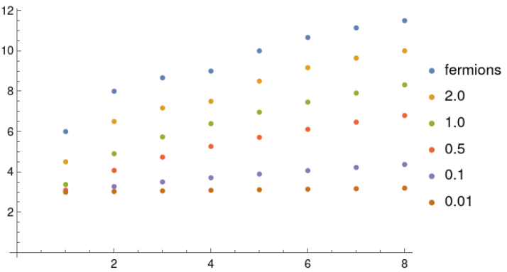
For internal widths of the composite bosons the external energy per composite boson is shown depending on the number of composite bosons. If they were perfect bosons the energy would be constant, if the fermions building the bosons were not coupled at all the value for “fermions” in an harmonic potential is added. With the parameter it is possible to tune the composite bosons from bosonic to fermionic character.
As we restricted our self to for the particle masses, we will compare this to a quantum harmonic oscillator with the same harmonic potential for both fermion types
with . The energy states are
for each fermion type, corresponding to the external energy 6 in the ground state with . In the limit of boson we do have and double force resulting in .
VI Short Discussion and Outlook
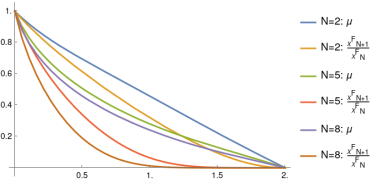
The composite bosons can be tuned from fermionic to bosonic behavior
| (2) |
with =0 in the fermionic case. They become better bosons (), if their internal width gets smaller. This might be used as a parameter indicating how bosonic the behavior of the system is. In figure (2) we compare it to the behavior of the c anhilation operator on the states from [1].
Composite bosons depend strongly on the dimension [3]. So we calculate fig (1) for lower dimensions in fig (3). In both cases of lower dimensionthe bosonic behavior is not shown. This effects are discussed in [3]. It seems that the handling in [1] are hiding some of the complexity of composite bosons, as no energies are involved in the analysis. This might be a motivation for using a toy system to quickly try different composite boson systems.
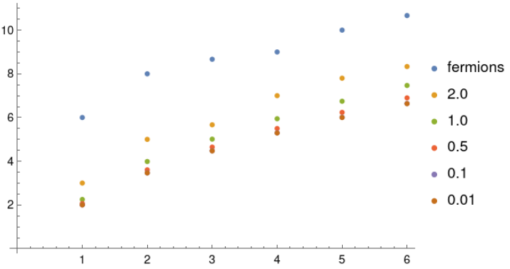
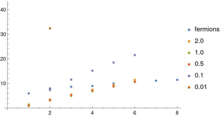
One can see, that in 2D (left) and 1D (right) the behavior is not boson like [3].
References
- [1] C. K. Law. Quantum entanglement as an interpretation of bosonic character in composite two-particle systems. Phys. Rev. A 71, 034306, 2005. https://arxiv.org/abs/quant-ph/0411040.
- [2] Luigi Amico, Rosario Fazio, Andreas Osterloh, and Vlatko Vedral. Entanglement in many-body systems. Rev. Mod. Phys. 80, 517, 2008. https://arxiv.org/abs/quant-ph/0703044.
- [3] Cecilia Cormick and Leonardo Ermann. Ground state of composite bosons in low-dimensional graphs. Phys. Rev. A, 107:043324, Apr 2023. https://arxiv.org/abs/2304.14834.