(eccv) Package eccv Warning: Package ‘hyperref’ is loaded with option ‘pagebackref’, which is *not* recommended for camera-ready version
Removing Reflections from RAW Photos
Abstract
We describe a system to remove real-world reflections from images for consumer photography. Our system operates on linear (RAW) photos, with the (optional) addition of a contextual photo looking in the opposite direction, e.g., using the “selfie” camera on a mobile device, which helps disambiguate what should be considered the reflection. The system is trained using synthetic mixtures of real-world RAW images, which are combined using a reflection simulation that is photometrically and geometrically accurate. Our system consists of a base model that accepts the captured photo and optional contextual photo as input, and runs at 256p, followed by an up-sampling model that transforms output 256p images to full resolution. The system can produce images for review at 1K in 4.5 to 6.5 seconds on a MacBook or iPhone 14 Pro. We test on RAW photos that were captured in the field and embody typical consumer photographs.
![[Uncaptioned image]](/html/2404.14414/assets/x1.png)
1 Introduction
Taking pictures through glass is difficult. Light reflects off of the glass and linearly mixes with the subject, creating a distraction. Photos from cars and airplanes show the cabin, photos from buildings include the ceiling lights, photos of paintings are covered by haze, and shots while window shopping are photo-bombed by the photographer themself—to name just a few cases.
Removing undesirable reflections is difficult due to the wide diversity of locations and circumstances in which they occur. Locations include shopping destinations (photos into stores and displays), traveling (photos from cars, trains, airplanes, ferries, and ships), buildings (photos from restaurants, hotels, conference centers, and houses), museums of art, history, and science (photos of paintings, sculptures, and artifacts; aquariums, zoos, and technology), and in special situations (eyeglasses, specular objects, and monitors or screens). In any location, many circumstances influence the reflection: time of day (dusk, dawn, midday, night), lighting (sunlight, overcast, incandescent, tungsten, LED, colored), scene semantics (trees, clouds, scenery; streets, cars, people), illuminant power (bright, dark), and scene appearance (complex textures or simple colors and shapes). These diverse factors introduce priors on reflections because glass is usually placed judiciously in the real world.
One reflection removal technique involves taking a second photo. A black material is placed behind the glass to allow only reflected light to reach the camera. If this reflection image, and the original mixture image, are stored in a format that preserves the linear relationship between pixel values and the scene luminance (e.g., RAW), then these two scene-referred images can be subtracted to recover the image that transmitted through the glass. This transmission image can be recovered because light mixes by addition in photosites on the sensor.
Removal-by-subtraction has been used extensively to create datasets [27, 48], but it fails if there is motion in the reflected scene, including lighting changes, which restricts where data is collected. Alternatively, a glass pane can be manually placed, but the scene and lighting are typically similar on both sides of the glass. As recently noted by Lei [27], training and evaluations on datasets that do not represent real use cases can be misleading.
This paper presents a reflection removal system for consumer photography that addresses the following requirements:
-
1.
Handle typical reflections in consumer photography.
-
2.
Minimize user interactions (steps, taps, strokes).
-
3.
Allow photo capture in a typical amount of time.
-
4.
Produce results on-screen for review in about 5 seconds.
-
5.
Produce results at the input image resolution.
-
6.
Facilitate editing for error correction and aesthetics.
Few previous works satisfy all of these, which affect design and evaluation. In particular, data should represent the expected use for the system. To address req. 1, we accurately synthesize images that obviate the capture of ground truth images that prior systems use. By training on such data, we avoid using datasets that are skewed to unrealistic situations that allow ground truth capture.
Specifically we use linear scene-referred images to simulate images with photometric and colorimetric calibration (e.g., RAW). Thus, if we synthetically combine a (presumed transmitted) image of a storefront with a (presumed reflected) image of sunlit buildings, the reflection will be brighter, typically bluer in white balance, but attenuated by the physically plausible reflectance of glass.
To address reqs. 2–4, we avoid using video, frame bursts, and stereo pairs. Instead, we accept a single optional contextual photo to help identify what created the reflection. This second photo does not need to be captured simultaneously, or registered with the original photograph. In fact, it could be captured by turning around, pointing away from the window, and snapping the shutter again.
To address req. 5, we design a novel upsampler with a flexible output resolution; upsampling is imperative and non-trivial, but largely disregarded in the literature. To meet req. 6 we output both reflection and transmission images so users can blend them to contend with the inevitable long tail of practical failures.
Contributions: this work describes methods to
-
1.
synthesize training images from which models can directly generalize;
-
2.
use a contextual photo to identify the reflection;
-
3.
remove reflections in about 5 seconds at resolution for review;
-
4.
remove reflections at typical full image resolutions.
The paper is organized into prior work (Sec. 2), reflection synthesis (Sec. 3), removal (Sec. 4), and results (Sec. 5); geometric simulation (Appendix B–C), data collection (Appendix D), modeling (Appendix E), and results (Appendix F).
2 Prior work
Removing reflections is a long-standing problem. Prior works have used multi-image capture and machine learning. Among the latter, upsampling low-resolution results is an important sub-problem. We survey each category.
Multiple input images. Prior methods use video [5, 16], image sequences [17, 30, 33, 38, 39, 42, 43, 54], flash [4, 26], near infrared [19], polarization [12, 25, 34, 52, 28], and dual pixel images [37], as well as light fields [49]. We use an optional and additional photo of the reflected scene (not of the glass) to identify the reflection. This contextual photo is any for which the camera is pointed at the reflected scene (e.g., the camera is turned as in a “selfie” camera).
Reflection synthesis. Prior methods are trained with heuristically mixed pairs of tone-mapped images [9, 20, 16, 31, 55, 47, 56, 21, 6, 11]. Such mixing is inaccurate, so non-linear methods have been used [51, 24]. Physically based methods nonetheless use tone-mapped images [24]. Successful methods however require ground truth images to train models that generalize [27], typically at approximately a a: ratio of synthetic and real [20, 27, 47, 58, 50, 29, 36, 32]. This ratio raises issues of dataset scale and diversity because ground truth capture is tedious and restrictive. The largest dataset of real images to-date [59] has 14,952 pairs (), but methods such as [20, 47, 58] require pre-training on much larger datasets which exceed (e.g., ImageNet [41]). We synthesize photometrically accurate images so ground truth training images are not needed, and train models from scratch on millions of reflection examples, which improves performance.
Removing high resolution reflections. Most methods operate at about pixels, and cannot be trivially scaled up. To be useful, systems must provide preview images at pixels, and final outputs of and larger. Prasad [36] use a base model at pixels, and an upsampler that outputs beyond pixels. Their system is fast, but we show that it re-introduces sharp residual reflections. We design an upsampler with similar performance that removes sharp reflections.
Inference on RAW images. Most prior methods apply reflection removal to -bit display-referred images, such as internet JPEGs. These images have typically been white-balanced, tone-mapped, denoised, sharpened, and compressed. We reframe dereflection as operating on scene-referred (RAW) images. Lei [26] subtract pairs of RAW images to suppress the reflection before converting to -bit for full removal. We operate on RAW end-to-end. RAW inputs improve prior methods, but our system outperforms them.
3 Reflection synthesis
Our pipeline for removing reflections uses a base model and an upsampler (Sec. 4) that are trained solely on simulated images, which overcomes the scaling bottleneck of needing to capture real reflections. We simulate reflections photometrically by summing pairs of scene-referred images, which are linear with respect to scene luminance. In contrast, images in most -bit formats are display-referred—non-linearly related to luminance. Scene-referred images originate from sensor data stored in RAW format, such as Adobe Digital Negative (DNG). The transformation of RAW data into display-referred images is described by Adobe Camera RAW (ACR), the DNG spec. [1] pp.99-104, and the DNG SDK [1] as follows:
-
1.
Linearize (e.g. remove vignetting and spatially-varying black levels)
-
2.
Demosaic
-
3.
Subtract the black level
-
4.
Convert to XYZ color
-
5.
White balance111ACR defines two possible paths to a white balanced image—we discuss this below.
-
6.
Convert to RGB color
-
7.
Dehaze, tone map (spatial adaptive highlights, shadows, clarity); enhance texture; adjust local contrast, hue, color tone, whites, and blacks.
-
8.
Gamma compress
Step 8 yields a finished image that can be stored in bits, but its pixel values are non-linearly related to scene luminance because Step 7 performs an array of proprietary, non-linear, and spatially varying effects that are not usefully modeled with a gamma curve as is often done [58, 52, 29]. Most importantly, realistic reflections cannot be simulated by summing pairs of finished images.
Which earlier step is most appropriate for simulation? The outputs of Steps 5 and 6 are linear, but the illuminant color has been removed by white balancing—accurate reflections cannot be simulated here because scenes that reflect from and transmit through glass are often illuminated by light sources with differing colors, and those colors mix before white balancing. The output of Step 3 is linear, preserves the illuminant color, and has been demosaicked, but colors are with respect to a sensor-specific spectral basis—images from different sensors cannot be summed here. The output of Step 4 is however ideal: the XYZ color space is sensor-independent, yet the illuminant color has not been removed (unlike prior works [2]), and pixels are linear with respect to luminance. We therefore select Step 4 and XYZ color space to simulate photometrically accurate reflections.
Note that the ACR steps (above) differ from many cameras and the literature [2, 7, 22], wherein white balance is applied before converting to XYZ with the forward matrix. ACR also supports that ordering (DNG Spec.[1] p103, matrix FM), but reflection simulation requires the opposite. Fortunately, ACR specifies a second path that uses color matrices (DNG Spec. [1] pp101-103, matrix CM), to transform to XYZ before white balancing. All DNGs are required to provide such color matrices, whereas the forward matrices of the first path are optional.222ACR recommends forward matrices under extreme lighting (DNG Spec. [1] pp.101-103), for which they are more precise. Reflection simulation however requires using color matrices. Both depend on the as-shot illuminant; see Funcs. A10, A5, A8. We therefore use the color matrix path. In Sec. 5, we show that this color processing yields synthetic training data with sufficient realism for models to generalize to photos in-the-wild from other cameras, while prior methods do not. Appendix G and Func. A4 detail how to extract these XYZ images using the DNG SDK [1].
3.1 Photometric reflection synthesis
Our most fundamental simulation principle is the additive property of light: glass superimposes the light field from a reflection and transmission scene to form a mixture. The resulting mixture image accumulates (with equal weight) photons from the transmission scene into a transmission image and a reflection image . We simulate and from images in linear XYZ color (ACR Step 4).
The first photometric property is illuminant color, which often differs between and because the glass in consumer photographs typically separates indoor and outdoor spaces. Otherwise, the photographer could walk around the glass to take their photo. Even in specialized scenes like museum display cases, the case is often internally illuminated, making its illuminant color different than in the gallery at large. By representing in XYZ color before white balancing, the illuminant colors are mixed.
The second property is the power of light. In typical scenes, the illuminant power differs on either side of the glass ( and differ in brightness). The number of photons that strike the sensor is scaled by the exposure , for shutter speed , aperture , and gain (ISO). We normalize the exposures of and so pixels are proportional to scene luminance up to a shared constant. This non-exposed mixture is , , and , for exposures and . We simulate a capture function that re-exposes and re-white balances by exposing the mean pixel to a target value , , , and , where is a matrix that white balances in XYZ (Func. A3, Sec. A.1). If pixels in or are saturated, , to ensure they remain so. Lastly, is converted to scene-referred, linear RGB to train dereflection models. See Sec. 4, Func. 1 and Appendix A for details.
Mixtures , above, are photometrically mixed, but they are not always useful. When saturation dictates the re-exposure , additional pixels can be clipped, modeling over-exposed . Images or can also be so dark that they are invisible, or so mutually destructive that one would struggle to identify the subject. These photos do not model that photographers care about. We therefore collect a large dataset of images and search for that yield well exposed and mixed . This search introduces photometric and semantic priors on , , and (e.g., skies often create reflections). See Appendix D for details.
3.2 Geometric reflection synthesis
Our second fundamental simulation principle is that we want the mixtures to be geometrically valid. Specifically, denoting the synthetic images to be added together as and our source image pairs as , we synthesize and by modeling Fresnel attenuation, perspective projection, double reflection, and defocus. We omit from effects related to global color, dirt, and scratches, since photo editing tools can correct them. We also model a physically calibrated amount of defocus blur, and find that most reflections are sharp as also noted in [27]. See Appendix B for details.
3.3 The contextual photo
We accept an optional contextual photo that directly captures the reflection scene to help identify the reflection . Capture of can be simultaneous with the secondary front camera (selfie) on a mobile device, or briefly later. We make three observations about the views of and (see Fig. A11):
-
1.
Even if the cameras are collocated, the viewpoints of and will be translated by twice the distance to the glass.
-
2.
If the mixture is captured obliquely to the glass, rotating the contextual view 180∘ yields little common content.
-
3.
If the front camera is used, the reflection scene might be partially occluded by the photographer.
Image will therefore often contain little matching content unless it is captured carefully. We minimize such burden by allowing to be any view of the reflection scene. Crucially, this relaxation also facilitates geometric simulation. We scalably model by cropping source images into a disjoint left/right half (or top/bottom). The contextual image encodes information about the lighting and scene semantics because we use the same capture function with the same white balance as . See Sec. 3.1, Func. 1, and Appendix C for details.
Input: A random pair of XYZ images
Output: Simulated components and context image.
4 Reflection removal
Our system removes reflections from RAW images, , in linear RGB color (ACR Step 6) with an optional context image that is white balanced like . See Func. 1. Both and share a scene-referred color space, which aids removal; RGB supports pre-trained perceptual losses. We predict and in linear RGB, and store inference outputs by inverting ACR steps 3–6 to produce new RAW images.
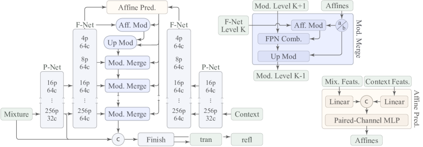
Our system uses two models. A base model operates on at pixels to predict (rectangular images are tiled and linearly blended). These outputs are passed to an upsampler that is applied at each level of a Gaussian pyramid. The models apply these conceptual steps: 1) inputs are projected to a higher, -dimensional space; 2) nonlinear, “semantic” per-pixel features are computed; 3) components and are identified in ; 4) output images are rendered. We implement these steps differently in each model.
4.1 Base model
The base model is illustrated in Fig. 2. A multi-scale feature backbone projects into a linear, high dimensional space and computes semantic features (labeled P-Net). The multi-resolution semantic features are fused (labeled F-Net) with a feature pyramid network (FPN) at the input resolution. We use EfficientNet as the backbone [44] at pixels and fuse features with a BiFPN pyramid [45, 53].
The context image , is processed identically to . Its lowest resolution FPN features are used to predict affines that progressively modify the FPN features of using conv-mod-deconv operations ala StyleGAN [23]. Modulation is per-channel because does not share identical content with . Conceptually, modulation gives the model additional capacity to identify in its features. A finishing module further identifies and renders (it is the head in [58]). We predict independently, rather than enforcing , to decouple failures. Training uses the losses of [58] with improvements to the adversary and gradient terms. Crucially, training is end-to-end from random weights. See Sec. E.1.
4.2 Upsampler
The upsampler, Fig. 3, is iteratively applied over a Gaussian pyramid. It first projects the low- and high-resolution images , and into a high dimensional space with a convolutional backbone. Critically, batch norms are omitted so the same transform is applied to and .
The upsampler first identifies features , in via feature masks. This matching process uses products of features: when activations match, their product can be large regardless of sign, whereas summation yields large activations if either input is large. We generalize this idea in a mask prediction module, Fig. 3 (bottom), which predicts affines to match and scale activations before a sigmoid is applied. Two per-pixel, per-channel masks are predicted, , . Errors are corrected by a joint predictor (a per-channel, per-pixel MLP; the affines are predicted similarly; see Sec. E.2 for details). Masks, , , are resampled and multiplied with to project its features into subspaces for , . By resampling masks, not features, sharp features are preserved. This key step assumes the identity , of the component to which each feature belongs is low frequency. Errors are corrected with finishing convolutions, which render .
5 Results
We compare the simulation, base model, and upsampler to prior methods.
5.1 Reflection simulation
Source images are drawn from MIT5K [8], RAISE [10], and Laval Indoors [14] for a total of , RAW images and , scene-referred Image-Based Lighting (IBL) panoramas. The IBLs are equivalent to about , indoor RAW images because we simulate random cameras (the expected FOV is , Sec. B.2, B.4). Images are grouped into , outdoor and (in mathematical expectation) , indoor images to create pairs , Sec. D.2. Indoor and outdoor images are split into train, validation, and test sets so no images are shared among the sets. We use for training and for test.
The number of examples is amplified by randomization in the geometric simulation (Appendix B, D). We search examples for useful . After culling, about mixtures remain, and we rendered at and pixels to train the base and upsampler models. The pixel dataset has ,, for training, , for test, and , for validation; the dataset has ,,, ,, and , (smaller due to resolution constraints).
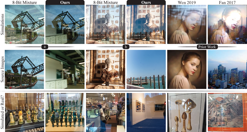
Fig. 4 shows results of mixing scene-referred images: (a) correct illuminant colors and (b) correct reflection visibility. We linearly blended -bit tone-mapped images for comparison, and compare to prior works (see caption).
Discussion. Prior works mix -bit tone-mapped images, and the results are qualitatively unrealistic. In particular, their simulated reflections overpower the highlights, and are not powerful enough in the shadows, which are boosted by tone mapping. By contrast, in our simulations light from two scenes is mixed linearly and equally without tone-mapping. This accurate mixing allows our system to generalize better to new scenes, and gives us SOTA performance without the need to train on real mixture images. Furthermore, by synthesizing photometrically and geometrically plausible mixture images, we naturally encode priors on the appearance of reflections in real-world scenes. For example, indoor light is typically relatively weak, so reflections from indoor scenes are typically of regions that are close to light sources (ceilings, etc.). These create small reflection regions that often look yellow when they appear over outdoor scenes, due to typical indoor illuminant colors. Conversely, outdoor light is powerful enough to bounce off diffuse objects, and have enough strength to create reflections of whole scenes that can be colorful, or blue in white balances due to the color of outdoor illuminants. Of course, at nighttime, whole indoor scenes can reflect over cityscapes, etc. These kinds of priors are apparent in consumer photos (see Figs. 1, 9, 9, A12, A13, A14). Lastly, like prior works we pair indoor/outdoor photos, which permits unlikely but plausible pairings such as bathrooms and beaches. Future work can remove such unlikely pairings if they prove unhelpful.
5.2 Base reflection removal
Base models were trained end-to-end from random weights at pixels using an Adam optimizer with -, discriminator -, and batch size over GPUs for epochs. Adversarial training begins after one epoch.
We trained three base models, one with and two without context . To omit , we remove the modulated merges (see Fig. 2), which removes generally useful model capacity. As a second alternative, the base architecture is not changed, and the model is trained and tested with random . We use this latter randomized approach for ablation. A third alternative, setting , forces the backbones to handle both natural and unnatural , and yields unreliable performance.
| Method | PSNRt | SSIMt | PSNRr | SSIMr | |
| Control | |||||
| Ours+ctx | |||||
| Ours | |||||
| DSRNet [20] | |||||
| Zhang [58] | |||||
| CoRRN [47] | |||||
| Abl. | Ours+rnd | ||||
| Ours+rac |
| Method | PSNRt | SSIMt | PSNRr | SSIMr | |
| GT | Control | ||||
| Ours | |||||
| Ours-NM | |||||
| VDSR+C | |||||
| VDSR | |||||
| E2E | Ours | ||||
| VDSR+C |
We compare to Zhang et al. [58], DSRNet [20], and CoRRN [47] by training their models on our dataset. Recall that our model uses the same losses and network head as Zhang et al. to simplify comparison to prior work. Tab. 2 shows that all methods improve images relative to the average degradation to (control). Our models outperform prior works (ours+ctx, ours). We ablate by using random (ours+rnd), which degrades performance, and this is statistically significant. Removing operations that use (ours) does not degrade performance compared to training with, and using, random (differences are not significant), which suggests the contextual model does not learn better priors with its additional capacity, but rather leverages the content of . Ablating further, using the reflection as the context () at test time only does not improve the contextual model performance (ours+rac), which suggests the model has learned to be appropriately sensitive to : the model does not require and to match, and it is robust to their differences because it is trained with disjoint crops (, ).
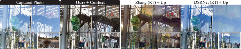
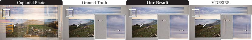
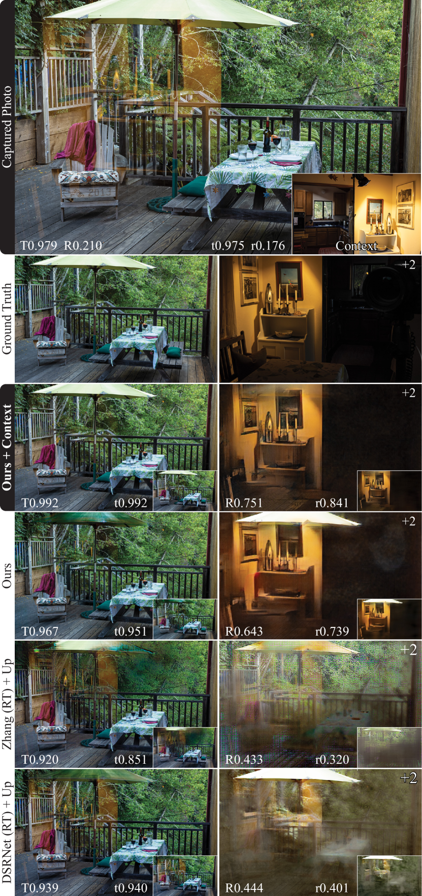
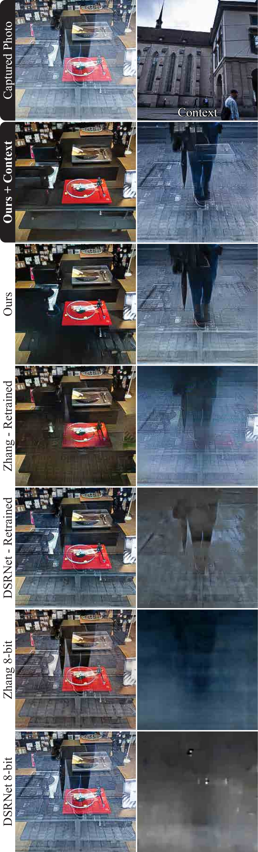
For visual comparison, we captured333We thank Florian Kainz for his help capturing these photos. ground truth reflections in three common cases: looking out of a house, looking into a display case, and photographing artwork Fig. 9 and Fig. A12. We dereflected with Zhang, DSRNet (retrained, RT), and our models at (inset images) and upsampled them to (see next section). The empirical SSIM values (lowercase t, r) are commensurate with test performance (Tab. 2). In Fig. 9 our contextual model separates the reflection, but without context our model attributes the colors in the umbrella with a reflected object. Prior works perform quantitatively worse.
In Figs. 1, 5, 9, A13, A14, and A15 we compare results on photos in-the-wild from cameras that were not used to construct the synthetic dataset. We also compare the published -bit models of Zhang and DSRNet (excepting Fig. 5). The 8-bit models do not recover most or , but generalize better when re-trained on our data (Figs. 9, A13, A14). These methods do not however recover well, which is needed for aesthetic and error corrections (see Sec. 5.4).
Our model has M parameters, while DSRNet has M. Inference at , takes / on a M1 MacBook Pro (Gb) and iPhone Pro.
Discussion. Our models recover in diverse real-world cases including museums, nature, shopping, a mid-day city, artwork, etc. (Figs. 1, 5, 9, 9, A12, A13, A14, A15). In Fig. 1 the contextual model yields more correct and uniform color on the Egyptian tablet by reducing ambiguity about the color of the reflection scene, which is typical (compare to inset w/o context). Failures occur when or is bright, and pushes the other into the noise floor, effectively saturating it to black. As reflections strengthen, the removal problem transitions from unmixing to hole filling. When a single color channel saturates, RAW images can preserve enough information to recover the lost content. Nonetheless, systems must address both sub-problems because users typically cannot control the strength of reflections.
Lastly, errors can occur when textured regions of and overlap, as in Fig. 1 where a stone wall overlaps with the dress of the subject. Color differences can help separate complex textures, as in Fig. 9 where the reflection of a painting is successfully separated from complex tree textures. Without such differences, overlapping textures corrupt , and models must repair or hallucinate the missing content as they might also do in saturated regions.
5.3 Upsampling
Our upsampler is trained using Adam with -, batch size over GPUs, and converges after about epochs. For end-to-end operation (E2E), we tune with the base model outputs for examples at -.
We compare to V-DESIRR [36] in Tab. 2 by upsampling the ground truth (GT) and using the base model (E2E). For best E2E performance, we fine tuned our upsampler and V-DESIRR with the base model. Our method performs best on and (ours). Cycle consistency loss improves V-DESIRR (+C), so we used this for E2E. We ablated the upsampler masking operations by using only the finisher head (Ours-NM); performance degraded almost to match V-DESIRR.
Comparing on GT images, Fig. 6 and Fig. A17, V-DESIRR produces strong artifacts, even after fine tuning (adding cycle-consistency losses did not help).
Inference of our E2E upsampler, up to preview size , takes and on our MacBook and iPhone (hardware details are in Sec. 5.2).
Discussion. V-DESIRR amplifies errors at low resolutions by repeatedly upsampling its previous output images. By contrast, our model masks and copies the mixture features to the outputs . This direct copy reduces error propagation. Errors can still occur when features that are not present in the low resolution inputs become visible at the next level upward (see Fig. A18). In such cases the low resolution cannot guide upsampling of such features, and the upsampler must infer the high resolution image to which the features belong.
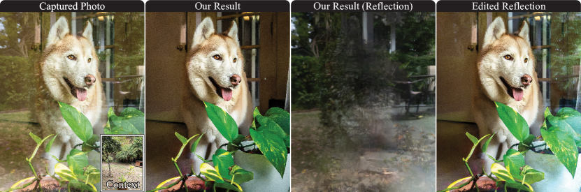
5.4 Reflection editing
In Fig. 7 and Fig. A19 we show that the predicted reflection facilitates aesthetic editing and error correction. In Fig. 7, the reflection color and spatial arrangement is modified. Error correction is shown in Fig. A19, Sec. F.4. Edits were made in Photoshop using the tone-mapped and images, and the “Linear Dodge (Add)” layer blend mode. We found that this is often sufficient, but editing tools should blend directly in linear RGB to enhance realism.
6 Conclusion
We have described a reflection removal system that is trained solely on mixture images that are created with a photometrically and geometrically accurate reflection simulation that uses scene-referred images. Moreover, we search among millions of these for well-exposed, visible, and visually interpretable that encode natural priors. Our system comprises a novel base model and upsampler that perform well on real images, even though we have not trained it on them.
Since Farid and Adelson [12], many signals have been used to remove reflections. We add illuminant color and contextual photos. Our system operates on RAW images end-to-end, which further and aids removal. Lastly, our system also has some ability to remove lens flares, though they are not in our dataset, Fig. A16. Flare removal systems might therefore be pre-trained to remove reflections and thus contend with the difficulty of capturing realistic lens flares.
References
- [1] Adobe: Adobe DNG specification. https://helpx.adobe.com/camera-raw/digital-negative.html (2024), accessed 2024-03-01
- [2] Afifi, M., Abdelhamed, A., Abuolaim, A., Punnappurath, A., Brown, M.S.: CIE XYZ net: Unprocessing images for low-level computer vision tasks. IEEE Trans. Pattern Anal. Mach. Intell. 44(9), 4688–4700 (2022). https://doi.org/10.1109/TPAMI.2021.3070580, https://doi.org/10.1109/TPAMI.2021.3070580
- [3] Afifi, M., Barron, J.T., LeGendre, C., Tsai, Y., Bleibel, F.: Cross-camera convolutional color constancy. In: 2021 IEEE/CVF International Conference on Computer Vision, ICCV 2021, Montreal, QC, Canada, October 10-17, 2021. pp. 1961–1970. IEEE (2021). https://doi.org/10.1109/ICCV48922.2021.00199, https://doi.org/10.1109/ICCV48922.2021.00199
- [4] Agrawal, A.K., Raskar, R., Nayar, S.K., Li, Y.: Removing photography artifacts using gradient projection and flash-exposure sampling. ACM Trans. Graph. 24(3), 828–835 (2005). https://doi.org/10.1145/1073204.1073269, https://doi.org/10.1145/1073204.1073269
- [5] Alayrac, J., Carreira, J., Zisserman, A.: The visual centrifuge: Model-free layered video representations. In: IEEE Conference on Computer Vision and Pattern Recognition, CVPR 2019, Long Beach, CA, USA, June 16-20, 2019. pp. 2457–2466. Computer Vision Foundation / IEEE (2019). https://doi.org/10.1109/CVPR.2019.00256, http://openaccess.thecvf.com/content_CVPR_2019/html/Alayrac_The_Visual_Centrifuge_Model-Free_Layered_Video_Representations_CVPR_2019_paper.html
- [6] Arvanitopoulos, N., Achanta, R., Süsstrunk, S.: Single image reflection suppression. In: 2017 IEEE Conference on Computer Vision and Pattern Recognition, CVPR 2017, Honolulu, HI, USA, July 21-26, 2017. pp. 1752–1760. IEEE Computer Society (2017). https://doi.org/10.1109/CVPR.2017.190, https://doi.org/10.1109/CVPR.2017.190
- [7] Brooks, T., Mildenhall, B., Xue, T., Chen, J., Sharlet, D., Barron, J.T.: Unprocessing images for learned raw denoising. In: IEEE Conference on Computer Vision and Pattern Recognition, CVPR 2019, Long Beach, CA, USA, June 16-20, 2019. pp. 11036–11045. Computer Vision Foundation / IEEE (2019). https://doi.org/10.1109/CVPR.2019.01129, http://openaccess.thecvf.com/content_CVPR_2019/html/Brooks_Unprocessing_Images_for_Learned_Raw_Denoising_CVPR_2019_paper.html
- [8] Bychkovsky, V., Paris, S., Chan, E., Durand, F.: Learning photographic global tonal adjustment with a database of input / output image pairs. In: The 24th IEEE Conference on Computer Vision and Pattern Recognition, CVPR 2011, Colorado Springs, CO, USA, 20-25 June 2011. pp. 97–104. IEEE Computer Society (2011). https://doi.org/10.1109/CVPR.2011.5995332, https://doi.org/10.1109/CVPR.2011.5995332
- [9] Chen, Z., Long, F., Qiu, Z., Zhang, J., Zha, Z., Yao, T., Luo, J.: A closer look at the reflection formulation in single image reflection removal. IEEE Trans. Image Process. 33, 625–638 (2024). https://doi.org/10.1109/TIP.2023.3347915, https://doi.org/10.1109/TIP.2023.3347915
- [10] Dang-Nguyen, D., Pasquini, C., Conotter, V., Boato, G.: RAISE: a raw images dataset for digital image forensics. In: Ooi, W.T., Feng, W., Liu, F. (eds.) Proceedings of the 6th ACM Multimedia Systems Conference, MMSys 2015, Portland, OR, USA, March 18-20, 2015. pp. 219–224. ACM (2015). https://doi.org/10.1145/2713168.2713194, https://doi.org/10.1145/2713168.2713194
- [11] Fan, Q., Yang, J., Hua, G., Chen, B., Wipf, D.P.: A generic deep architecture for single image reflection removal and image smoothing. In: IEEE International Conference on Computer Vision, ICCV 2017, Venice, Italy, October 22-29, 2017. pp. 3258–3267. IEEE Computer Society (2017). https://doi.org/10.1109/ICCV.2017.351, https://doi.org/10.1109/ICCV.2017.351
- [12] Farid, H., Adelson, E.H.: Separating reflections and lighting using independent components analysis. In: 1999 Conference on Computer Vision and Pattern Recognition (CVPR ’99), 23-25 June 1999, Ft. Collins, CO, USA. pp. 1262–1267. IEEE Computer Society (1999). https://doi.org/10.1109/CVPR.1999.786949, https://doi.org/10.1109/CVPR.1999.786949
- [13] Farid, H., Simoncelli, E.P.: Differentiation of discrete multidimensional signals. IEEE Trans. Image Process. 13(4), 496–508 (2004). https://doi.org/10.1109/TIP.2004.823819, https://doi.org/10.1109/TIP.2004.823819
- [14] Gardner, M., Sunkavalli, K., Yumer, E., Shen, X., Gambaretto, E., Gagné, C., Lalonde, J.: Learning to predict indoor illumination from a single image. ACM Trans. Graph. 36(6), 176:1–176:14 (2017). https://doi.org/10.1145/3130800.3130891, https://doi.org/10.1145/3130800.3130891
- [15] Goldberg, N.: Camera Technology: The Dark Side of the Lens. Elsevier Science (1992), https://books.google.com/books?id=g7NvF2jWcp8C
- [16] Guo, X., Cao, X., Ma, Y.: Robust separation of reflection from multiple images. In: 2014 IEEE Conference on Computer Vision and Pattern Recognition, CVPR 2014, Columbus, OH, USA, June 23-28, 2014. pp. 2195–2202. IEEE Computer Society (2014). https://doi.org/10.1109/CVPR.2014.281, https://doi.org/10.1109/CVPR.2014.281
- [17] Han, B., Sim, J.: Reflection removal using low-rank matrix completion. In: 2017 IEEE Conference on Computer Vision and Pattern Recognition, CVPR 2017, Honolulu, HI, USA, July 21-26, 2017. pp. 3872–3880. IEEE Computer Society (2017). https://doi.org/10.1109/CVPR.2017.412, https://doi.org/10.1109/CVPR.2017.412
- [18] Hold-Geoffroy, Y., Sunkavalli, K., Eisenmann, J., Fisher, M., Gambaretto, E., Hadap, S., Lalonde, J.: A perceptual measure for deep single image camera calibration. In: 2018 IEEE Conference on Computer Vision and Pattern Recognition, CVPR 2018, Salt Lake City, UT, USA, June 18-22, 2018. pp. 2354–2363. Computer Vision Foundation / IEEE Computer Society (2018). https://doi.org/10.1109/CVPR.2018.00250, http://openaccess.thecvf.com/content_cvpr_2018/html/Hold-Geoffroy_A_Perceptual_Measure_CVPR_2018_paper.html
- [19] Hong, Y., Lyu, Y., Li, S., Shi, B.: Near-infrared image guided reflection removal. In: IEEE International Conference on Multimedia and Expo, ICME 2020, London, UK, July 6-10, 2020. pp. 1–6. IEEE (2020). https://doi.org/10.1109/ICME46284.2020.9102937, https://doi.org/10.1109/ICME46284.2020.9102937
- [20] Hu, Q., Guo, X.: Single image reflection separation via component synergy. In: IEEE/CVF International Conference on Computer Vision, ICCV 2023, Paris, France, October 1-6, 2023. pp. 13092–13101. IEEE (2023). https://doi.org/10.1109/ICCV51070.2023.01208, https://doi.org/10.1109/ICCV51070.2023.01208
- [21] Jin, M., Süsstrunk, S., Favaro, P.: Learning to see through reflections. In: 2018 IEEE International Conference on Computational Photography, ICCP 2018, Pittsburgh, PA, USA, May 4-6, 2018. pp. 1–12. IEEE Computer Society (2018). https://doi.org/10.1109/ICCPHOT.2018.8368464, https://doi.org/10.1109/ICCPHOT.2018.8368464
- [22] Karaimer, H.C., Brown, M.S.: A software platform for manipulating the camera imaging pipeline. In: Leibe, B., Matas, J., Sebe, N., Welling, M. (eds.) Computer Vision - ECCV 2016 - 14th European Conference, Amsterdam, The Netherlands, October 11-14, 2016, Proceedings, Part I. Lecture Notes in Computer Science, vol. 9905, pp. 429–444. Springer (2016). https://doi.org/10.1007/978-3-319-46448-0_26, https://doi.org/10.1007/978-3-319-46448-0_26
- [23] Karras, T., Aittala, M., Hellsten, J., Laine, S., Lehtinen, J., Aila, T.: Training generative adversarial networks with limited data. In: Larochelle, H., Ranzato, M., Hadsell, R., Balcan, M., Lin, H. (eds.) Advances in Neural Information Processing Systems 33: Annual Conference on Neural Information Processing Systems 2020, NeurIPS 2020, December 6-12, 2020, virtual (2020), https://proceedings.neurips.cc/paper/2020/hash/8d30aa96e72440759f74bd2306c1fa3d-Abstract.html
- [24] Kim, S., Huo, Y., Yoon, S.: Single image reflection removal with physically-based training images. In: 2020 IEEE/CVF Conference on Computer Vision and Pattern Recognition, CVPR 2020, Seattle, WA, USA, June 13-19, 2020. pp. 5163–5172. Computer Vision Foundation / IEEE (2020). https://doi.org/10.1109/CVPR42600.2020.00521, https://openaccess.thecvf.com/content_CVPR_2020/html/Kim_Single_Image_Reflection_Removal_With_Physically-Based_Training_Images_CVPR_2020_paper.html
- [25] Kong, N., Tai, Y., Shin, J.S.: A physically-based approach to reflection separation: From physical modeling to constrained optimization. IEEE Trans. Pattern Anal. Mach. Intell. 36(2), 209–221 (2014). https://doi.org/10.1109/TPAMI.2013.45, https://doi.org/10.1109/TPAMI.2013.45
- [26] Lei, C., Chen, Q.: Robust reflection removal with reflection-free flash-only cues. In: IEEE Conference on Computer Vision and Pattern Recognition, CVPR 2021, virtual, June 19-25, 2021. pp. 14811–14820. Computer Vision Foundation / IEEE (2021). https://doi.org/10.1109/CVPR46437.2021.01457, https://openaccess.thecvf.com/content/CVPR2021/html/Lei_Robust_Reflection_Removal_With_Reflection-Free_Flash-Only_Cues_CVPR_2021_paper.html
- [27] Lei, C., Huang, X., Qi, C., Zhao, Y., Sun, W., Yan, Q., Chen, Q.: A categorized reflection removal dataset with diverse real-world scenes. In: IEEE/CVF Conference on Computer Vision and Pattern Recognition Workshops, CVPR Workshops 2022, New Orleans, LA, USA, June 19-20, 2022. pp. 3039–3047. IEEE (2022). https://doi.org/10.1109/CVPRW56347.2022.00343, https://doi.org/10.1109/CVPRW56347.2022.00343
- [28] Lei, C., Huang, X., Zhang, M., Yan, Q., Sun, W., Chen, Q.: Polarized reflection removal with perfect alignment in the wild. In: 2020 IEEE/CVF Conference on Computer Vision and Pattern Recognition, CVPR 2020, Seattle, WA, USA, June 13-19, 2020. pp. 1747–1755. Computer Vision Foundation / IEEE (2020). https://doi.org/10.1109/CVPR42600.2020.00182, https://openaccess.thecvf.com/content_CVPR_2020/html/Lei_Polarized_Reflection_Removal_With_Perfect_Alignment_in_the_Wild_CVPR_2020_paper.html
- [29] Li, C., Yang, Y., He, K., Lin, S., Hopcroft, J.E.: Single image reflection removal through cascaded refinement. In: 2020 IEEE/CVF Conference on Computer Vision and Pattern Recognition, CVPR 2020, Seattle, WA, USA, June 13-19, 2020. pp. 3562–3571. Computer Vision Foundation / IEEE (2020). https://doi.org/10.1109/CVPR42600.2020.00362, https://openaccess.thecvf.com/content_CVPR_2020/html/Li_Single_Image_Reflection_Removal_Through_Cascaded_Refinement_CVPR_2020_paper.html
- [30] Li, Y., Brown, M.S.: Exploiting reflection change for automatic reflection removal. In: IEEE International Conference on Computer Vision, ICCV 2013, Sydney, Australia, December 1-8, 2013. pp. 2432–2439. IEEE Computer Society (2013). https://doi.org/10.1109/ICCV.2013.302, https://doi.org/10.1109/ICCV.2013.302
- [31] Li, Y., Brown, M.S.: Single image layer separation using relative smoothness. In: 2014 IEEE Conference on Computer Vision and Pattern Recognition, CVPR 2014, Columbus, OH, USA, June 23-28, 2014. pp. 2752–2759. IEEE Computer Society (2014). https://doi.org/10.1109/CVPR.2014.346, https://doi.org/10.1109/CVPR.2014.346
- [32] Li, Y., Liu, M., Yi, Y., Li, Q., Ren, D., Zuo, W.: Two-stage single image reflection removal with reflection-aware guidance. Appl. Intell. 53(16), 19433–19448 (2023). https://doi.org/10.1007/S10489-022-04391-6, https://doi.org/10.1007/s10489-022-04391-6
- [33] Liu, Y., Lai, W., Yang, M., Chuang, Y., Huang, J.: Learning to see through obstructions. In: 2020 IEEE/CVF Conference on Computer Vision and Pattern Recognition, CVPR 2020, Seattle, WA, USA, June 13-19, 2020. pp. 14203–14212. Computer Vision Foundation / IEEE (2020). https://doi.org/10.1109/CVPR42600.2020.01422, https://openaccess.thecvf.com/content_CVPR_2020/html/Liu_Learning_to_See_Through_Obstructions_CVPR_2020_paper.html
- [34] Lyu, Y., Cui, Z., Li, S., Pollefeys, M., Shi, B.: Reflection separation using a pair of unpolarized and polarized images. In: Wallach, H.M., Larochelle, H., Beygelzimer, A., d’Alché-Buc, F., Fox, E.B., Garnett, R. (eds.) Advances in Neural Information Processing Systems 32: Annual Conference on Neural Information Processing Systems 2019, NeurIPS 2019, December 8-14, 2019, Vancouver, BC, Canada. pp. 14532–14542 (2019), https://proceedings.neurips.cc/paper/2019/hash/d47bf0af618a3523a226ed7cada85ce3-Abstract.html
- [35] Mechrez, R., Talmi, I., Zelnik-Manor, L.: The contextual loss for image transformation with non-aligned data. In: Ferrari, V., Hebert, M., Sminchisescu, C., Weiss, Y. (eds.) Computer Vision - ECCV 2018 - 15th European Conference, Munich, Germany, September 8-14, 2018, Proceedings, Part XIV. Lecture Notes in Computer Science, vol. 11218, pp. 800–815. Springer (2018). https://doi.org/10.1007/978-3-030-01264-9_47, https://doi.org/10.1007/978-3-030-01264-9_47
- [36] Prasad, B.H.P., S, G.R.K., Lokesh, R.B., Mitra, K., Chowdhury, S.: V-DESIRR: very fast deep embedded single image reflection removal. In: 2021 IEEE/CVF International Conference on Computer Vision, ICCV 2021, Montreal, QC, Canada, October 10-17, 2021. pp. 2370–2379. IEEE (2021). https://doi.org/10.1109/ICCV48922.2021.00239, https://doi.org/10.1109/ICCV48922.2021.00239
- [37] Punnappurath, A., Brown, M.S.: Reflection removal using a dual-pixel sensor. In: IEEE Conference on Computer Vision and Pattern Recognition, CVPR 2019, Long Beach, CA, USA, June 16-20, 2019. pp. 1556–1565. Computer Vision Foundation / IEEE (2019). https://doi.org/10.1109/CVPR.2019.00165, http://openaccess.thecvf.com/content_CVPR_2019/html/Punnappurath_Reflection_Removal_Using_a_Dual-Pixel_Sensor_CVPR_2019_paper.html
- [38] Sarel, B., Irani, M.: Separating transparent layers through layer information exchange. In: Pajdla, T., Matas, J. (eds.) Computer Vision - ECCV 2004, 8th European Conference on Computer Vision, Prague, Czech Republic, May 11-14, 2004. Proceedings, Part IV. Lecture Notes in Computer Science, vol. 3024, pp. 328–341. Springer (2004). https://doi.org/10.1007/978-3-540-24673-2_27, https://doi.org/10.1007/978-3-540-24673-2_27
- [39] Sarel, B., Irani, M.: Separating transparent layers of repetitive dynamic behaviors. In: 10th IEEE International Conference on Computer Vision (ICCV 2005), 17-20 October 2005, Beijing, China. pp. 26–32. IEEE Computer Society (2005). https://doi.org/10.1109/ICCV.2005.216, https://doi.org/10.1109/ICCV.2005.216
- [40] Shih, Y., Krishnan, D., Durand, F., Freeman, W.T.: Reflection removal using ghosting cues. In: IEEE Conference on Computer Vision and Pattern Recognition, CVPR 2015, Boston, MA, USA, June 7-12, 2015. pp. 3193–3201. IEEE Computer Society (2015). https://doi.org/10.1109/CVPR.2015.7298939, https://doi.org/10.1109/CVPR.2015.7298939
- [41] Simonyan, K., Zisserman, A.: Very deep convolutional networks for large-scale image recognition. In: Bengio, Y., LeCun, Y. (eds.) 3rd International Conference on Learning Representations, ICLR 2015, San Diego, CA, USA, May 7-9, 2015, Conference Track Proceedings (2015), http://arxiv.org/abs/1409.1556
- [42] Sun, C., Liu, S., Yang, T., Zeng, B., Wang, Z., Liu, G.: Automatic reflection removal using gradient intensity and motion cues. In: Hanjalic, A., Snoek, C., Worring, M., Bulterman, D.C.A., Huet, B., Kelliher, A., Kompatsiaris, Y., Li, J. (eds.) Proceedings of the 2016 ACM Conference on Multimedia Conference, MM 2016, Amsterdam, The Netherlands, October 15-19, 2016. pp. 466–470. ACM (2016). https://doi.org/10.1145/2964284.2967264, https://doi.org/10.1145/2964284.2967264
- [43] Szeliski, R., Avidan, S., Anandan, P.: Layer extraction from multiple images containing reflections and transparency. In: 2000 Conference on Computer Vision and Pattern Recognition (CVPR 2000), 13-15 June 2000, Hilton Head, SC, USA. p. 1246. IEEE Computer Society (2000). https://doi.org/10.1109/CVPR.2000.855826, https://doi.org/10.1109/CVPR.2000.855826
- [44] Tan, M., Le, Q.V.: Efficientnet: Rethinking model scaling for convolutional neural networks. In: Chaudhuri, K., Salakhutdinov, R. (eds.) Proceedings of the 36th International Conference on Machine Learning, ICML 2019, 9-15 June 2019, Long Beach, California, USA. Proceedings of Machine Learning Research, vol. 97, pp. 6105–6114. PMLR (2019), http://proceedings.mlr.press/v97/tan19a.html
- [45] Tan, M., Pang, R., Le, Q.V.: Efficientdet: Scalable and efficient object detection. In: 2020 IEEE/CVF Conference on Computer Vision and Pattern Recognition, CVPR 2020, Seattle, WA, USA, June 13-19, 2020. pp. 10778–10787. Computer Vision Foundation / IEEE (2020). https://doi.org/10.1109/CVPR42600.2020.01079, https://openaccess.thecvf.com/content_CVPR_2020/html/Tan_EfficientDet_Scalable_and_Efficient_Object_Detection_CVPR_2020_paper.html
- [46] Thompson, R.: Identification of glass samples by their refractive index. https://www.asdlib.org/onlineArticles/elabware/thompson/Glass/Glass(RI)PFaculty.pdf (2023), accessed 2023-11-10
- [47] Wan, R., Shi, B., Li, H., Duan, L., Tan, A., Kot, A.C.: Corrn: Cooperative reflection removal network. IEEE Trans. Pattern Anal. Mach. Intell. 42(12), 2969–2982 (2020). https://doi.org/10.1109/TPAMI.2019.2921574, https://doi.org/10.1109/TPAMI.2019.2921574
- [48] Wan, R., Shi, B., Li, H., Hong, Y., Duan, L., Kot, A.C.: Benchmarking single-image reflection removal algorithms. IEEE Trans. Pattern Anal. Mach. Intell. 45(2), 1424–1441 (2023). https://doi.org/10.1109/TPAMI.2022.3168560, https://doi.org/10.1109/TPAMI.2022.3168560
- [49] Wang, Q., Lin, H., Ma, Y., Kang, S.B., Yu, J.: Automatic layer separation using light field imaging. CoRR abs/1506.04721 (2015), http://arxiv.org/abs/1506.04721
- [50] Wei, K., Yang, J., Fu, Y., Wipf, D.P., Huang, H.: Single image reflection removal exploiting misaligned training data and network enhancements. In: IEEE Conference on Computer Vision and Pattern Recognition, CVPR 2019, Long Beach, CA, USA, June 16-20, 2019. pp. 8178–8187. Computer Vision Foundation / IEEE (2019). https://doi.org/10.1109/CVPR.2019.00837, http://openaccess.thecvf.com/content_CVPR_2019/html/Wei_Single_Image_Reflection_Removal_Exploiting_Misaligned_Training_Data_and_Network_CVPR_2019_paper.html
- [51] Wen, Q., Tan, Y., Qin, J., Liu, W., Han, G., He, S.: Single image reflection removal beyond linearity. In: IEEE Conference on Computer Vision and Pattern Recognition, CVPR 2019, Long Beach, CA, USA, June 16-20, 2019. pp. 3771–3779. Computer Vision Foundation / IEEE (2019). https://doi.org/10.1109/CVPR.2019.00389, http://openaccess.thecvf.com/content_CVPR_2019/html/Wen_Single_Image_Reflection_Removal_Beyond_Linearity_CVPR_2019_paper.html
- [52] Wieschollek, P., Gallo, O., Gu, J., Kautz, J.: Separating reflection and transmission images in the wild. In: Ferrari, V., Hebert, M., Sminchisescu, C., Weiss, Y. (eds.) Computer Vision - ECCV 2018 - 15th European Conference, Munich, Germany, September 8-14, 2018, Proceedings, Part XIII. Lecture Notes in Computer Science, vol. 11217, pp. 90–105. Springer (2018). https://doi.org/10.1007/978-3-030-01261-8_6, https://doi.org/10.1007/978-3-030-01261-8_6
- [53] Wightman, R.: Pytorch image models. https://github.com/huggingface/pytorch-image-models (2019). https://doi.org/10.5281/zenodo.4414861
- [54] Xue, T., Rubinstein, M., Liu, C., Freeman, W.T.: A computational approach for obstruction-free photography. ACM Trans. Graph. 34(4), 79:1–79:11 (2015). https://doi.org/10.1145/2766940, https://doi.org/10.1145/2766940
- [55] Yang, J., Gong, D., Liu, L., Shi, Q.: Seeing deeply and bidirectionally: A deep learning approach for single image reflection removal. In: Ferrari, V., Hebert, M., Sminchisescu, C., Weiss, Y. (eds.) Computer Vision - ECCV 2018 - 15th European Conference, Munich, Germany, September 8-14, 2018, Proceedings, Part III. Lecture Notes in Computer Science, vol. 11207, pp. 675–691. Springer (2018). https://doi.org/10.1007/978-3-030-01219-9_40, https://doi.org/10.1007/978-3-030-01219-9_40
- [56] Yang, Y., Ma, W., Zheng, Y., Cai, J., Xu, W.: Fast single image reflection suppression via convex optimization. In: IEEE Conference on Computer Vision and Pattern Recognition, CVPR 2019, Long Beach, CA, USA, June 16-20, 2019. pp. 8141–8149. Computer Vision Foundation / IEEE (2019). https://doi.org/10.1109/CVPR.2019.00833, http://openaccess.thecvf.com/content_CVPR_2019/html/Yang_Fast_Single_Image_Reflection_Suppression_via_Convex_Optimization_CVPR_2019_paper.html
- [57] Zhang, R., Isola, P., Efros, A.A., Shechtman, E., Wang, O.: The unreasonable effectiveness of deep features as a perceptual metric. In: 2018 IEEE Conference on Computer Vision and Pattern Recognition, CVPR 2018, Salt Lake City, UT, USA, June 18-22, 2018. pp. 586–595. Computer Vision Foundation / IEEE Computer Society (2018). https://doi.org/10.1109/CVPR.2018.00068, http://openaccess.thecvf.com/content_cvpr_2018/html/Zhang_The_Unreasonable_Effectiveness_CVPR_2018_paper.html
- [58] Zhang, X.C., Ng, R., Chen, Q.: Single image reflection separation with perceptual losses. In: 2018 IEEE Conference on Computer Vision and Pattern Recognition, CVPR 2018, Salt Lake City, UT, USA, June 18-22, 2018. pp. 4786–4794. Computer Vision Foundation / IEEE Computer Society (2018). https://doi.org/10.1109/CVPR.2018.00503, http://openaccess.thecvf.com/content_cvpr_2018/html/Zhang_Single_Image_Reflection_CVPR_2018_paper.html
- [59] Zhu, Y., Fu, X., Jiang, P., Zhang, H., Sun, Q., Chen, J., Zha, Z., Li, B.: Revisiting single image reflection removal in the wild. CoRR abs/2311.17320 (2023). https://doi.org/10.48550/ARXIV.2311.17320, https://doi.org/10.48550/arXiv.2311.17320
Removing Reflections from RAW Photos
Supplementary Material
Eric Kee Adam Pikielny Kevin Blackburn-Matzen Marc Levoy
Appendix A Photometric reflection synthesis
As part of our photometric reflection synthesis pipeline, Func. 1, we compute a new exposure and white balance for the simulated mixture image, , using Func. A2 and Func. A3, respectively. These functions follow ACR color processing, and use methods in the Adobe DNG SDK, Appendix G. The ACR color processing that produces XYZ source images is specified in Func. A4 and discussed in Appendix G.
A.1 White balancing
To compute a new white balance within Func. A3, we use the C5 white balancer of Afifi et al. [3]. C5 white balances an input image by using an additional sample images that were captured from the same camera. We therefore cache samples for each camera in the dataset of RAW images, and remove all images for which there were not samples from the camera ( is the C5 default).
Input: A simulated mixture image and its associated component images
Output: An exposure value
White balancing with C5 requires that simulated mixtures in XYZ be transformed into camera color space. In Func. A3 we use the XYZ_to_CAM transform associated with the RAW source image of to simulate a camera from which the mixture was captured, since typically dominates in the sum due to attenuation by the glass (see Appendix B). The white balancer produces a new white point WhiteCAM_awb in camera color space. We then follow ACR color processing of white points in camera color space by transforming WhiteCAM_awb into XY coordinates and computing a new XYZ_to_CAM transform using DNG SDK Func. A8. This new transform into XYZ is then composed with Bradford adaptation (Func. A3 line 5) to construct a single, linear white balancing transform that operates on images in XYZ space (line 6).
Input: A re-exposed XYZ mixture, , and the transmission
Output: XYZ_to_XYZ_awb
Over a large scale dataset, white balancer failures inevitably occur. These are handled by culling if the new white point is extremely different from the as-shot WhiteXY of . Extreme changes to the true white point are not common because reflections that are of practical interest are either transparent, localized, or both. The new XY white point (WhiteXY_awb) can be further restricted to lie on the Planckian locus, and we found this to be sufficient for our source images, which were captured under typical illuminants. Projection from WhiteCAM_awb to WhiteXY_awb can be done using ACR Func. A11 and A8, or Func. A9 with the Planckian constraint, as noted in Func. A3, line 4.
In summary, the white balance computed in Func. A3 is a linear transform, which we denote XYZ_to_XYZ_awb, that composes three ACR color transforms: 1) it maps images into the camera color space of , 2) it maps back to XYZ under a new white point, and 3) it applies Bradford adaptation to the D50 illuminant. In the simulation (Func. 1) this transform is applied to , , , and so they are interpreted with respect to the same white point, lines 8-9.
Appendix B Geometric reflection synthesis
As part of our reflection removal pipeline, a geometric simulation is used to construct transmission and reflection pairs of images from a dataset of pairs of scene-referred (RAW) photographs that were not captured with or through glass. These transmission and reflection pairs are then added together to form the training data for our models, with ground truth provided by the constituent images in each pair. This simulation approach overcomes the scaling bottleneck of capturing real reflection images for training, which is difficult because ground truth (without the glass present) is not readily available.
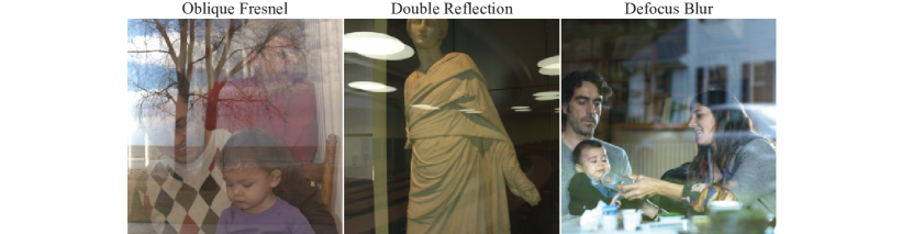
In particular, we synthesize transmission images and reflection images as functions of and that appropriately model Fresnel attenuation, perspective projection, double reflection, and defocus blur. Examples are shown in Fig. A10. We omit from effects related to global color, dirt, and scratches since existing photo editing tools are well equipped to correct them after reflection removal.
B.1 Fresnel attenuation
Fresnel attenuation is the most essential property to simulate because it reduces the intensity of the reflected image. Specifically, reflections are attenuated by a spatially varying factor that depends on the angle of incidence at which light strikes the glass with respect to the surface normal vector. As derived in [25],
where , and is the refractive index of glass. For , , Fresnel attenuation factors account for up to stops (underexposure), and gradually strengthen to stop at .
To specify , we define images as originating from a mirror surface, with incident rays reaching the camera by the law of reflection. In the next section we decribe how to simulate a diversity of practical geometric configurations of the glass and camera to construct and thus compute . Glass also attenuates the transmission by . This is typically close to , but at extreme angles it creates a visible darkening effect.
B.2 Camera projection
We model consumer photography applications in which one sees a subject partially visible behind glass and takes a picture of it. This constrains the relative pose of the camera and glass, and introduces natural priors on the location and appearance of reflections. For example, skies typically reflect near the top of images, and reflections are typically stronger at the edges of photos where the camera rays strike the glass at a relatively higher angle of incidence, .
Inclination angle . Most glass is approximately vertical, so if the viewpoint of looks upward, the viewpoint of should as well. We use a pose estimator [18], and augment the search for realistic pairings , Sec. 3.1, by checking if is below a maximum absolute value. In addition to this inclination discrepancy filter, images are culled if their inclination angle exceeds a threshold.
Roll angle . Images are culled if their estimated roll exceeds a maximum absolute value as these typically indicate that the pose estimator has failed.
Field of view. Images are also culled if the estimated vertical FOV is zero, which indicates general pose estimation failures. Otherwise we randomly sample , where is the uniform distribution.
Azimuth angle . Most glass in consumer photography is roughly planar. We constrain the camera azimuth with respect to the glass so that the camera rays strike this plane (accounting for the FOV). We randomly sample .
B.3 Defocus blur
Recently Lei [27] found that performance of state-of-the-art methods degrades significantly for sharp reflections due to an imbalance of blurry images in training and testing data. Physically based methods have been developed to introduce realistic defocus blur using depth maps [24], but this introduces a data collection bottleneck by requiring RGBD cameras that also have physical limitations. We instead model a physically based prior on the amount of defocus blur.
Defocus blurs are determined by the camera focus depth, aperture, and focal length. Points on an object at depth that differs from the focus depth project to a circular region with diameter ,
| (1) |
where is the focal length, and is the aperture f-number. This circle of confusion [15] is magnified with increasing focal length or decreasing N.
Defocused images are simulated by sampling diameters (mm) for the circle of confusion. The focal length (mm) and aperture (dimensionless) are sampled according to their physical ranges in mobile cameras. The object and focus depths and (feet) are sampled , in the plausible and finite range of scene depths to which is sensitive. The diameter (mm) is converted to a percentage of the sensor height, (the minimum sensor dimension). Reflections are blurred by convolving them with a circular defocus kernel with pixel diameter , where is the minimum dimension of the image in pixels. We maintain this physical calibration when images are cropped into halves to simulate contextual views (Sec. 3.3 and Appendix C).
B.4 HDR Environment sampling
A dataset of indoor HDR Image-Based-Lights (IBLs) are used as an additional source of scene-referred images [14]. Artificial light sources in HDR images are typically not saturated, which makes it possible to simulate reflections of light sources that are not saturated (or, under-exposed RAW images could be used).
When one of the images in a pair is an IBL, a synthetic camera is constructed with a pose that matches the RAW image to which it is paired (see Sec. B.2), excepting that the azimuth is sampled independently and uniformly at random in . Contextual images are simulated by a second synthetic camera within the IBL with an adjacent, non-overlapping FOV.
The IBLs [14] are captured under a fixed white point, which allows for the color of the illuminant (i.e., its white balance) to be mixed correctly with the RAW data. We calibrate the exposure of these indoor IBLs by setting their median intensity to match the median value of all indoor RAW images (the median contends with saturated pixels). This cropped HDR image can be photometrically combined, and geometrically transformed using functions or .
B.5 Double reflection
Glass panes introduce multiple reflective surfaces that create a double reflection or “ghosting” effect. Shih et al. [40] ascribe this to the thickness of a single or double pane, and show shifts up to pixels for thicknesses in 3–10mm under some viewing distances, but double reflections are often much larger. Gaps between panes reach mm as reported commercially, and each pane adds up to mm. These multiple reflecting surfaces are also not necessarily parallel, uniformly thick, or flat as assumed in [40]. These factors produce significant double reflections even in modern windows, including when the camera is distant. We simulate these complex effects by adopting the geometric model of [40] and allowing a greater range of thicknesses, 8–20mm. We uniformly sample a glass thickness, physical viewing distance, and refractive index. These facilitate a ray tracing procedure, detailed below.
The primary reflection that contributes to is determined by the Fresnel attenuation as described in Sec. B.1. Specifically, the intensity of light at each homogeneous image coordinate is , because we have defined as encoding the light along the incident rays with where is the angle of incidence. We simulate a second reflection by tracing the camera rays through a simulated single pane of uniform thickness to identify the coordinates at which they would emerge from the glass after being internally reflected from the back surface of the pane. Coordinates are shifted according to their transit distance within the glass, which is determined by the law of reflection and Snell’s law. We neglect the latter as insignificant in comparison to the former and the various non-modeled physical effects of real glass panes. Under these assumptions, rays that enter the glass at emerge at in direction . An image is needed to describe the intensity of incident light in direction at , but because we have defined as describing the light reflected from a corresponding direction . Since we do not have , we assume that the light field is sufficiently smooth that , since is small. We therefore warp such that , and combine this warped image with to produce a double reflection image.
The double reflection image is given by , where is the known Fresnel attenuation due to the primary reflection (see Sec. B.1), and specifies the attenuation of the rays that travel into the glass before they are internally reflected back to the camera. These latter rays encounter three surfaces, and lose intensity at each one. The first surface is the front face of the glass, where they are mildly attenuated by as they transmit into the glass. Second is the back face, where they reflect and are attenuated again according to their angle of incidence, which has been altered by Snell’s law. This change of incidence angle however has a negligible effect on the the Fresnel attenuation factor within the typical incidence ranges. We therefore use as the attenuation at the second surface. Lastly, the rays re-encounter the front face of the glass (now from within) where they transmit out of the glass and are attenuated again by approximately . This gives .
Fig. A10 shows an example of a simulated double reflection, selected to show a case when the primary and secondary reflections are significantly shifted. We note that no doubling effect can occur along the direction of the glass surface normal because the rays that enter the glass re-emerge after internal reflection at the same location they entered. Thus double reflection fields that follow our geometric model (and the model of [40]), in which there are two perfectly parallel planes, must exhibit a radial pattern around the image of the glass surface normal. These patterns are not always apparent in practice, which suggests that the geometrical arrangement of glass surfaces that is described by Shih [40] omits important factors. We nonetheless adopt their model as being sufficient because visible reflections are typically localized to regions of an image, which obscures the presence or absence of a radial center.
Appendix C The contextual photo
One arrangement of a primary and a contextual camera is shown in Fig. A11 (see caption for explanation). This specific arrangement of cameras is neither required nor typical in practice, but it reveals general geometric differences between the views of primary and contextual cameras. The view of the so-called reflection camera is translated by , twice the distance to the glass. Furthermore, if the contextual camera is rotated from the primary, the latter view will be in an opposite direction. At extreme rotations, the views will have little or no overlap.
Because the translation and rotation of the contextual camera view can differ significantly from the primary camera, it is difficult to simulate a contextual view using a dataset of image pairs and that are used to create mixture images from the perspective of a primary camera. In particular, content from should not be copied into a simulated contextual image , as trained models could learn to cheat by searching for patches of that have the same perspective projection in . Such patches will not be present in practice.
We create a scalably large dataset of contextual images by noting that will often contain no common content with unless the photographer is asked to
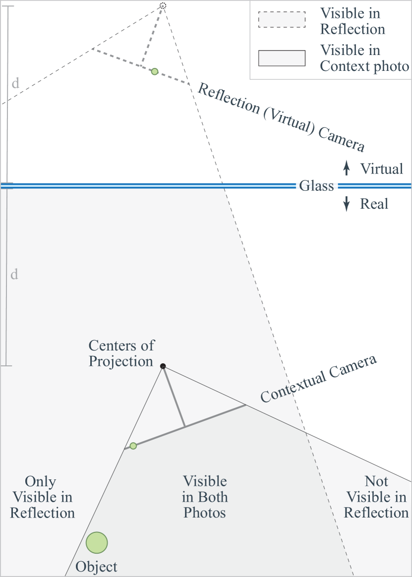
point the camera at what they see in the reflection. We minimize such burden on the photographer, and define the contextual image as any image of the reflection scene that does not view the same parts of the scene as . This definition allows contextual images to capture lighting information (sunlight, incandescent, etc.) and scene semantics (outdoor, indoor, city, nature, etc.) to aid reflection removal.
To construct , we crop reflection source images, , into non-overlapping left/right or top/bottom squares , and similarly for transmission source images . This yields four pairs for simulation for all . The mixture and context images are , where , and . We fix the capture function for both and to have the same white balance so can describe the color of the reflection scene in addition to its semantics.
Appendix D Data collection
Below are the data search and collection methods summarized in Sec. 3.1.
D.1 Mixture search
Well-exposed mixtures are identified by checking if the mean pixel value is within a normal distribution over the pixel values in the dataset of RAW images.
Well mixed are identified by computing the SSIM between and as a block-wise image, and checking if the mean of this SSIM image is within a useful range: if the SSIM is too high, the reflection is imperceptible; if it is too low, the mixture is not visually interpretable, even by a human. We compute this single channel SSIM image as a weighted average of the corresponding per-channel SSIM images. The weights are the average value in each color channel, which better accounts for strongly colored images. Lastly, the standard deviation of this single channel SSIM image is checked to remove reflections that are imperceptible, but nonetheless produce a low mean SSIM by spreading their power broadly (they have low spatial variance).
D.2 Source images
We collect all images at their native RAW camera resolution to facilitate training upsampling methods. We label all images, including IBLs (Sec. B.4), as outdoor and indoor since glass typically separates indoor and outdoor spaces. This information is available in existing datasets [8, 10, 14], and can be collected at large scales via crowd-sourcing. We define our dataset of pairs for simulation as , where is all pairs . The set is uncommon, and should be included sparingly following empirical priors. We omit them.
D.3 Simulation settings
Two capture scenarios are generated for each pair . A virtual camera is posed randomly with maximum azimuth toward the glass and , where denotes the uniform distribution. Pairs are culled if , or either image has absolute inclination value or roll (see Sec. B.2). Lastly, capture scenarios are also culled if the camera rays from more than pixels do not strike the glass (they are parallel or divergent). This final check ensures that the glass fills the FOV.
We compute spatially varying Fresnel attenuation with index of refraction [46]; see Sec. B.1. Double reflections are simulated with glass thickness (mm) in at distances (mm) in , with probability of being a double pane; see Sec. B.5. Defocus blur is simulated with object and focus distances (ft) in with aperture and focal length of iPhone main cameras, and mm (mm equivalent units); see Sec. B.3. Simulated mixtures are culled if the mean SSIM between and falls outside of , or if the standard deviation of this SSIM is below ; see Sec. D.1.
Appendix E Reflection removal
Here we provide details of the base model architecture, as summarized in Sec. 4.1, and the upsampler, Sec. 4.2.
E.1 Base model
The base model is designed to leverage local and global features, Fig. 2, and produce pixel outputs in about second on a mobile device to meet req. 4 (see Sec. 1).
A feature backbone [44] is used to project into a linear, high dimensional space (-D) and compute semantic features (labeled P-Net). Features are at a variety of spatial and channel resolutions: , , , , . These features include the outputs of the initial convolution layer of the EfficientNet-B1 variant of [44] (as implemented by [53]), which we modify to use an initial stride of rather than so no initial down-sampling is performed on the input pixel images.
The multi-resolution feature tensors from the backbone are next fused into channels at the input resolution using the D0 variant of the EfficientDet feature pyramid architecture [45, 53] (labeled F-Net). This architecture first augments the input features with three additional levels: , , , where each results from a maxpool with stride , and the first is preceded by a conv, batch norm, and no activation. The augmented input features are then input to a series of so-called BiFPN layers [45] (see Fig. 3), which fuse features from low resolution to high, and then back to low resolution, in a zigzag operation that is repeated three times. To obtain high resolution fused features at only the input resolution of , we add a fourth repetition in which we omit the final high-to-low pass. We furthermore modify the low-to-high pass to incorporate the contextual image, as described next.
The contextual image, , is passed through the same F-Net and P-Net using the same weights as . The features of and at the lowest resolution are input to an affine prediction module, Fig. 2 (lower right). This module first vectorizes its two inputs, and passes them through a fully connected layer to transform them into two - vectors. These vectors embody pairs of channels, which we concatenate and input to an MLP (labeled paired-channel MLP) that predicts affine transforms that modify the features of the FPN during the final low-to-high pass.
The paired-channel MLP is a series of grouped convolutions that implement independent MLPs followed by a fully connected layer. These MLPs each have inputs, hidden, and output dimension, with leaky ReLUs after each layer. The inputs to these MLPs are corresponding pairs of channels from and . The outputs compose a single - vector that is input to a fully connected layer to predict affine transforms, two for each of the channels and levels of the FPN.444Note that we include two levels at pixels, in correspondence with the resolutions of the features that we extract from the backbone. Conceptually, this paired-channel MLP has the capacity to compare and to identify channels that match with the reflection scene, and to determine how to transform those channels to aid reflection removal.
The predicted affines from the paired-channel MLP are used in the final low-to-high pass of the FPN to perform a series of modulated merge operations, Fig. 2 (upper right). These merge operations use two affine transforms per feature channel, labeled and in Fig. 2. Transforms are used to perform a conv-mod-deconv operation ala StyleGan [23] on the features of from FPN level . These features are subsequently combined with the features from level by resampling the latter features and using fast normalized fusion [45] (labeled FPN Combine). These combined features are modified with a second conv-mod-deconv operation using the second group of affines, .
The final modulated merge produces - features at pixels. These features are concatenated with and the features from the first layer, for a total of channels. A convolutional finishing module is then applied. This module has the capacity to further identify and finally render and . To simplify comparison to prior work, our finishing module is the head in [58]. The first layer is , and projects the input features to dimensions, which are maintained throughout the remaining operations. Those operations are convolutions at dilation rates , each followed by a batch norm and leaky ReLU. A final convolution generates channels: and .
The model is trained using the perceptual, adversarial, and gradient losses of Zhang et al. [58] with a ResNet-based discriminator [23], and optimized 5-tap derivatives [13] in the exclusion loss to suppress grid artifacts. We also adopt the reflection loss of [58] to minimize arbitrary differences to prior work. Perceptual losses are computed in non-linear sRGB by applying gamma compression and using VGG19 features, weighted to contribute equally. Crucially, we train end-to-end from randomly initialized weights.
E.2 Upsampler
The upsampler architecture is summarized in Sec. 4.2 and Fig. 3. It transforms low resolution outputs , from the base model to a flexible output resolution. We use a Gaussian pyramid and apply the same upsampler at each level, Fig. 3. The upsampler projects the low resolution, -channel inputs into a high dimensional space using convolutions in an expand-and-contract pattern. We use kernels for feature expansion, and kernels for contraction. There are layers with hidden dimensions . We use leaky ReLU nonlinearities between the hidden layers, and no skip connections. Batch norms are omitted to facilitate a feature matching process, described next.
The components and are separated by identifying low resolution features and in the low resolution mixture . We predict , per-pixel, per-channel low resolution masks using a mask prediction module, Fig. 3 (bottom), which uses a paired-channel MLP (defined in Sec. E.1) to predict its affine transforms (see also Sec. 4.2). The joint mask predictor also uses a paired-channel MLP, but it directly outputs the final masks rather than affine transforms. The input, hidden, and output dimensions of both paired-channel MLPs are . The final layer is fully connected. As noted in Sec. E.1, these MLPs can be implemented efficiently as a series of grouped convolutions.
The finishing network is a series of convolutions that are distinguished by the number of channels and dilation rates, :, :, :. A final convolution produces the channels of output for and .
The upsampler is trained using a cycle-consistency loss on the predicted transmission and reflection, in addition to the losses of Pawan et al. [36]. Perceptual features are computed by converting to non-linear sRGB. For each predicted high resolution image the loss is a weighted sum of the following terms: , , , and , where downsamples to compute the cycle consistency loss, and denotes expectation over spatial dimensions and (where applicable) the output of the gradient operator. We use both the and norms to avoid introducing arbitrary differences to prior work [36]. The norms are weighted , gradient terms , LPIPS , and cycle consistency . These losses are accumulated over three upsampling levels from to pixels (smaller than the pixel output size of the base model to contend with memory constraints during training). The upsampler is trained first on the ground truth low resolution inputs, and fine tuned on the output of the base de-reflection model. When fine tuning, the pixel outputs of the base model are downsampled to 1282 pixels. At test time, no downsampling is applied. The upsampler takes pixel images as input, and produces output at pixels and higher.
Appendix F Results
Here we provide results and discussion in addition to Sec. 5.
F.1 Evaluation methods
Ground truth capture. Mixture images were captured with ground truth by placing a black material behind the glass and taking a second photo. Images were computed in linear sRGB after normalizing the exposures and using the white point of (see ACR Step 6, Sec. 3). Nonetheless, we found it necessary to capture and with fixed exposures and white points to avoid imprecisions in the values that are stored in RAW metadata.
SSIM computation. We report SSIM values between pairs of RAW images by first transforming them into linear sRGB (ACR Step 6, Sec. 3) using the white point of . By using a consistent white balance, across the ground truth , , and , we penalize errors in the white balance of the estimated and . For SSIM computation, images are then converted to non-linear sRGB by applying standard gamma compression (ACR Step 8):
where are pixel values in a linear sRGB image. We omit tone mapping operations (ACR Step 7) to remove subjectivity from the SSIM values. Lastly, SSIMs are reported as averages over the low-resolution images (denoted t, r) and high-resolution images (denoted T, R).
Ground truth photographs. Ground truth images were captured in three common scenarios: 1) looking out of a home window, Fig. 9; 2) photographing artwork, Fig. A12 (left); and 3) looking into a display case, Fig. A12 (right). In scenario one, the illuminant in the reflection scene is approximately ,, and the white point of the mixture image is ,. In scenario two, these values are , and ,, and in scenario three they are , and ,.
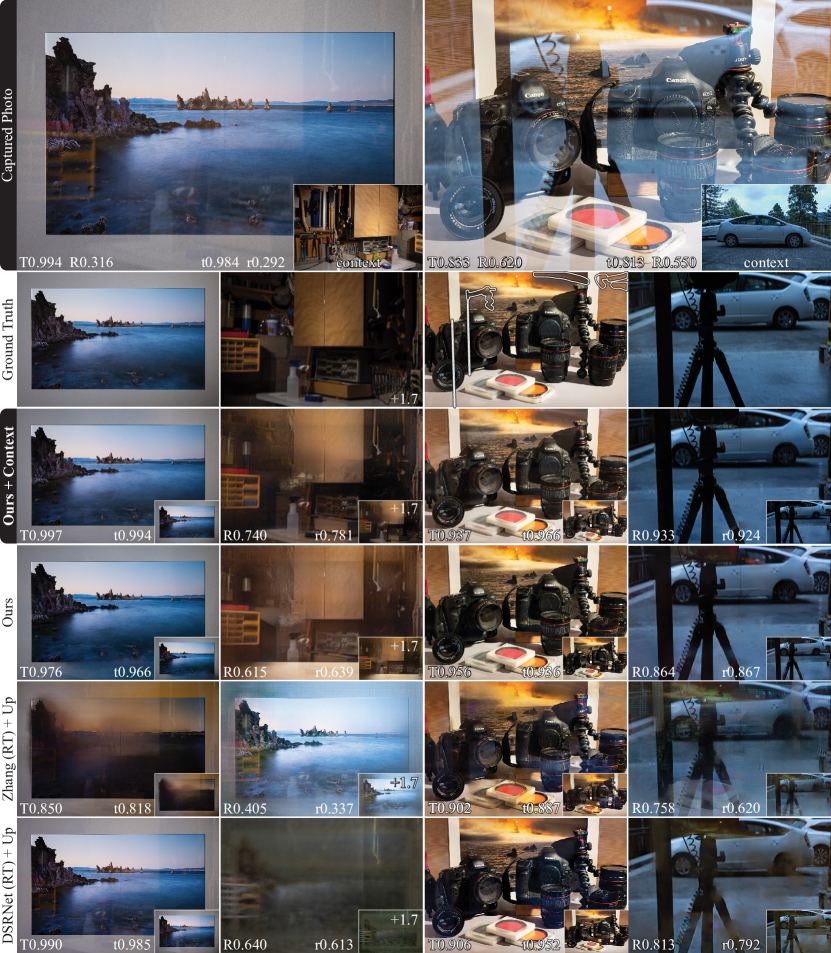
F.2 Base model comparisons
Reflections with ground truth. In Fig. A12 we show two images with ground truth reflections: photographing artwork, and looking into a display case. These complement Fig. 9, in which a photo was taken when looking out of a home window. The home window view includes an interior reflection that is strongly yellow due to the indoor illuminant color. In contrast, the artwork in Fig. A12 is illuminated by the same light source as the reflection scene, which produces a correctly white balanced reflection that consequently has more diverse colors. In contrast, the display case in Fig. A12 (right) reflects an outdoor scene with a very different white balance, which produces a reflection with a strong blue color cast. This outdoor reflection is visible over broad regions because the illuminant is powerful enough to reflect off of the diffuse ground and sidewalk surfaces with sufficient intensity to be clearly visible over the contents of the display case. These exterior reflections are also qualitatively different from those in photo of the artwork, where the reflection is sparse. The SSIM of the artwork is therefore high on average (), but the reflections are locally strong, whereas the SSIM of the display case is low () because the reflection affects broad regions.
Our base models improve the SSIM of and in all of these ground truth examples (labeled in lower case t, r), and this extends to the upsampled results (labeled in uppercase T, R) whereas prior works do not perform as well (Fig. A12 and Fig. 9). Our contextual model produces a more correct transmission and reflection image on the artwork. On the display case, the contextual model improves the reflection, whereas the cars are not fully removed from the transmission. We believe this variation results from saturated regions in the sky of the contextual photo, where we use the as-shot illuminant color in the EXIF to recover the color of the saturated pixels. Lastly, the method of Zhang [58] associates blue colored content with the reflection in both of these images, but this is incorrect for the painting; the transmission image is consequently distorted.
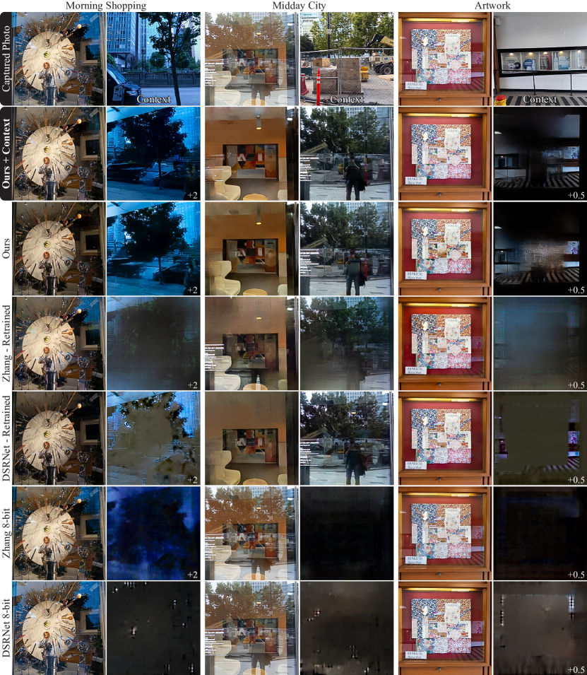
We found that our model removes blue colored reflections consistently well, and we believe that this results from their commonness (outdoor illuminants are powerful and therefore frequently create reflections that appear blue when mixed with interior scenes). The yellow color of interior reflections on outdoor scenes also seems to help, as our model can separate textured objects like the painting on the wall in Fig. 9 from the tree texture. We also tried illuminating the indoor scene in Fig. 9 with a special studio light that is much more powerful than a typical interior light source. This created a warm indoor reflection that was analogous to the display case in Fig. A12 (right), where the reflection covers large parts of the transmission scene. Our model results are less consistent in this artificial situation. We believe this is because it is rare for interiors to be flooded with such strong lights, and so their reflections are uncommon in our training data. We find that interior reflections tend to appear in small regions because most artificial light sources are weak—only objects near the light will be bright enough to reflect over outdoor scenes. At nighttime, however, consumer illuminants easily reflect over dark cityscapes. We found that our model results are less consistent on such images. This can be improved by augmenting the dataset with source images that were taken at nighttime.
Reflections in the wild. In Fig. A13, A14, and Fig. 9 we show results on reflections that were captured in-the-wild, where it was not possible to capture ground truth: (left) shopping in the morning, (middle) looking into a building at midday in a city, and (right) photographing artwork in an outdoor mall (Fig. A13); while traveling and photographing artwork from a city street (A14). We compare to Zhang [58] and DSRNet [20] using their published -bit models (bottom two rows). The -bit models do not consistently remove in-the-wild reflections, with the exception that the method of Zhang et al. seems to have learned to remove blue colored content (left); see also Fig. A15 (top). We retrained these prior works on our photometrically accurate training data (marked “retrained”), and they improve significantly. This suggests that the muted response of the -bit models on in-the-wild reflections results from differences between their training data and real world reflections, and furthermore that the training process of prior works is insufficient: pre-training on photometrically inaccurate images, and fine-tuning on small datasets of ground truth reflections does not produce models that generalize as well. Looking closely, however, note that the retrained models do still introduce blur and colored artifacts.
Our methods perform well across these diverse in-the-wild use cases. In Fig. A13, both our contextual and non-contextual models separate the strongly blue colored reflection, the complex cityscape reflection, and the artwork reflection (in the entrance to an indoor shopping mall). The contextual model improves each of these cases, excepting the transmission image for the shopping photo. We believe this also results from the saturated regions in the upper right of the contextual photo, where we have used the as-shot illuminant color in the EXIF to recover the pixels.
The midday city photo represents a difficult reflection, and both of our models improve this image. The result of the contextual model is more correct: the interior mural is more accurately reconstructed, and the white sign that is adhered to the glass is left more intact. Saturated regions near the ceiling have color artifacts in both cases.
Lastly, the artwork example (right) has two illuminants, a small warm colored artificial light, and a dominant outdoor illuminant. The white balance of the image is determined by the outdoor illuminant, which also illuminates the reflection scene, and this leads to a diversely colored reflection that both of our models are able to remove. The contextual model better preserves the texture of the artwork, and does not associate that texture with the reflection, whereas the non-contextual model does.
Subtle reflections. In Fig. A15 we show results on images with subtle reflections, which are common in art museums where the glass and lighting are optimized to reduce reflections. Our models are able to remove these reflections, and recover even when it is invisible to the naked eye. In the painting (Rembrandt’s “St. Matthew and the Angel”), the recovered reflection has a strong blue color
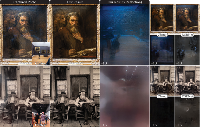
due to the special glass that is used in museums, and it correctly depicts the photographer and gallery. The colors in the recovered painting are also more correct. The specular reflection from the surface of the painting (top) is not removed, and we believe that this is the desired result. We have found that our models will sometimes remove sharp specular regions that are similar in color to the reflection from the glass, and this is visible in the upper quarter of the reflection image, where some specular texture from the surface of the painting is visible, and has been removed from the transmission.
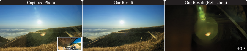
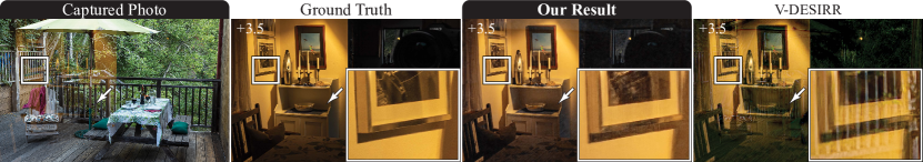
In Fig. A15 (bottom) we remove reflections from Ansel Adams’ “Residents of Hornitos.” Ceiling light sources are visible at the top of the photo, and on the left there is a general loss of contrast. The recovered transmission image has accurately uniform contrast, and the reflection reveals the hidden image of the photographer holding their cell phone. Our model is able to recover hidden reflections like this in part due to the bit depth of RAW images. The reflection is also blurry and differs in color.
Lens flares. Our model can also remove lens flares, which are reflections from the optical elements within the camera lens. An example is shown in Fig. A16. Most of the lens flare is removed, excepting one saturated region. The flare itself is also recovered in the reflection image even though the simulated reflections in the training dataset do not include lens flares. Since our method has some ability to generalize to flare removal, and it is difficult to create training data for flare removal, it could be helpful to pre-train flare removal methods first to remove photometrically accurate simulated reflections.
F.3 Upsampler comparisons
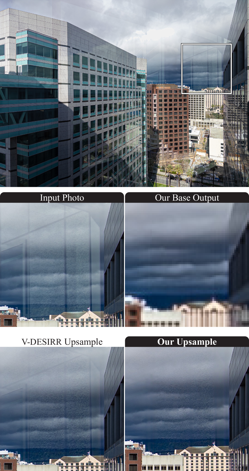
In Fig. A17 we provide additional comparison to V-DESIRR [36] in which we upsample a ground truth reflection image (a transmission image is upsampled in Fig. 6). A magnified region is inset, and shows that our method preserves details of a framed photo through the upsampling process, whereas V-DESIRR re-introduces the reflection content (the bars of a fence; see captured photo, white box). In the rest of the image, V-DESIRR introduces strong color artifacts around sharp edges. This is a consistent issue that appears to result from the propagation and amplification of small errors that are made at low resolutions. Our model reduces error propagation by masking and out of the high-resolution mixture features at each level. We are able to predict an effective, high resolution mask with a lightweight and fast model by matching features, whereas V-DESIRR must use its model capacity to infer from the high-resolution mixture image what details to add into the low resolution clean images. This latter problem is more difficult to solve with limited model capacity, and it is difficult to avoid propagating errors once they are made.
In Fig. A18 we show a typical failure mode of our model. The input image (top and center left) has a reflection of a textured exterior wall. Our base model correctly removes this reflection at pixels (center right). Notice that, at low resolution, it is possible to represent the vertical edges of the exterior wall, but not the texture of the wall. We upsampled this result with both V-DESIRR and our model. V-DESIRR re-introduces the low frequency edges that were removed by the base model, and it copies the high frequency wall texture into the transmission as well. Our model does not re-introduce the low frequency edges, but the high frequency texture of the wall that is not present at low resolution is copied into the transmission image. This produces a texture artifact in the final result. Future work should reduce these kinds of errors while keeping the architecture lightweight. This might be done by reusing feature information from the base model, and across levels of the Gaussian pyramid as the upsampler is iteratively applied.
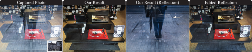
F.4 Editing reflections
In Fig. 7 and Fig. A19 we show examples of reflection editing for aesthetic control and error correction (see also Sec. 5.4). For Fig. A19, a photographer was asked to finish the photo using the outputs of the reflection removal system. They chose to re-introduce the reflection for aesthetic purposes, and to correct errors. The reflections from the edges of the top record player cover were removed by our system (white arrows); the photographer pulled them back into their edited image. Editing was performed in Photoshop using the tone-mapped transmission and reflection images, and the “Linear Dodge (Add)” layer blend mode.
Appendix G Adobe Camera RAW, DNG SDK
Here we detail the code within the DNG SDK [1] version 1.7.1 that is used in our simulation functions Func. 1, Func. A2 and Func. A3. In this work, the necessary SDK functionality was transliterated into Python to interoperate with the geometric simulation (Appendix B) and mixture search (Appendix D). To simplify the exposition, we however describe the SDK code here in a functional manner, whereas the SDK is a class system. Consequently, some of the SDK functions use class member variables, and not all functions in this exposition of the code map one-to-one with functions of the same name in the SDK.
As discussed in Sec. 3 and Appendix A, reflections are simulated in XYZ color space by using the color processing of the DNG SDK, which supports two paths to a white balanced, linear RGB image: the ForwardMatrix or the ColorMatrix. Only the latter path facilitates conversion to a device-independent color space (XYZ) before white balancing, as required for reflection simulation. We therefore implement in Func. A4 the ACR color process in which the ColorMatrix is used (cf. Func. A5). Note that both paths account for the as-shot illuminant because the ColorMatrix is interpolated according to the as-shot illuminant (see Func. A10 and Func. A8).
All supporting DNG SDK functions are listed below.
Input: A RAW image
Output: A linear image in XYZ color
Input: WhiteXY
Output: Transform to linear RGB
This function is included here as reference to the entire computation of the color transform to linear RGB. Note, the DNG SDK implements the DNG Spec. [1]. It uses the ForwardMatrix when it is available, and otherwise uses the CameraMatrix. In this work we use only the CameraMatrix, since this supports white balancing after conversion to XYZ.
Input: A DNG file
Output: The black level
The Stage-3 black level is not stored in the DNG EXIF header. It is a global scalar offset that remains after spatially varying black levels have been removed by parsing and applying the black level tags. By default, the DNG SDK Stage-3 image has a black level of zero, and negative noise values have been clipped to zero. In this work, we adopt that convention and clip the negative noise for simplicity. Clipping can however be disabled, and the non-zero Stage-3 black level can be recovered with a minor modification to the dng_validate binary, described below. The black level can then be read from the printed output of dng_validate when the stage-3 image is extracted with the -3 option.
Input: An image in camera color space
Output: Image with clipped higlights repaired
Input: White point XY
Output: Matrix XYZ_to_CAM
Input: An AWB white point in camera color space.
Output: XYZ_to_CAM_awb and WhiteXY_awb
Input: DNG AsShotXY XOR AsShotNeutral {All DNGs have one xor the other.}
Output: White point in XY
Input: DNG AsShotNeutral value
Output: An XY coordinate
Input: None
Output: The transform from XYZ D50 to linear sRGB.
Input: Two white points, w1 to w2.
Output: Bradford adaptation matrix.
Input: None
Output: XY coordinate of the D50 illuminant
Input: A scalar temperature value, .
Output: An XY coordinate.
Input: An XY vaue.
Output: An XYZ value
Input: A gamma compressed sRGB value
Output: A linear sRGB value