Learning H-Infinity Locomotion Control

Abstract

Stable locomotion in precipitous environments is an essential capability of quadruped robots, demanding the ability to resist various external disturbances. However, recent learning-based policies only use basic domain randomization to improve the robustness of learned policies, which cannot guarantee that the robot has adequate disturbance resistance capabilities. In this paper, we propose to model the learning process as an adversarial interaction between the actor and a newly introduced disturber and ensure their optimization with $H_{\infty}$ constraint. In contrast to the actor that maximizes the discounted overall reward, the disturber is responsible for generating effective external forces and is optimized by maximizing the error between the task reward and its oracle, i.e., “cost” in each iteration. To keep joint optimization between the actor and the disturber stable, our $H_{\infty}$ constraint mandates the bound of ratio between the cost to the intensity of the external forces. Through reciprocal interaction throughout the training phase, the actor can acquire the capability to navigate increasingly complex physical disturbances. We verify the robustness of our approach on quadrupedal locomotion tasks with Unitree Aliengo robot, and also a more challenging task with Unitree A1 robot, where the quadruped is expected to perform locomotion merely on its hind legs as if it is a bipedal robot. The simulated quantitative results show improvement against baselines, demonstrating the effectiveness of the method and each design choice. On the other hand, real-robot experiments qualitatively exhibit how robust the policy is when interfering with various disturbances on various terrains, including stairs, high platforms, slopes, and slippery terrains. All code, checkpoints, and real-world deployment guidance will be made public.

I Introduction

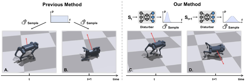
Figure 1: In traditional methods, the external forces are drawn from a fixed uniform distribution throughout the whole training process, which is less effective as the disturbance can not adapt to the performance level of the behavior policy. For example, a mild force is too easy to offset for a well-trained robot with strong stability (Fig. A), while exerting strong forces on the robot during early training may disrupt policy learning (Fig. B). This prompts us to design a disturber taking into account the performance level of the behavior policy. Thus we introduce a disturber to decide the external forces at each timestep. It is supposed to affect the robot to the extent that the robot shows an obvious performance drop but is still able to recover from this disturbance.

Recent end-to-end quadruped controllers exhibit various capabilities during deployment in real-world settings [9, 37, 40, 20, 19, 2, 22, 11, 16, 7, 8, 38, 39]. Characterized by learning from massive simulated data and sim-to-real transfer, these neural controllers enable legged robots to perform agile locomotion across diverse terrains, showing performance comparable to traditional methods [14, 10, 27]. Moreover, the learning-based approach enables skills beyond locomotion including target tracking in a bipedal manner [33, 15], manipulation using front legs [4], jumping over obstacles [33] and parkour [5].

To guarantee the effectiveness of these robots in real-world applications, it is extremely important that the controllers are robust against various disturbances. For instance, in scenarios such as disaster relief and field exploration, quadruped robots can be vulnerable to unforeseen external factors, such as severe wind conditions and falling debris, which may compromise their functionality. Previous learning-based controllers improve the robustness by incorporating domain randomization techniques [26, 35], which introduces perturbations to the robot during its training process. External forces, typically sampled from a uniform distribution, are applied to the robot [41, 23], enabling it to learn how to maintain stability in face of these circumstances.

However, the method is very basic and cannot completely ensure that the robot has adequate disturbance resistance capabilities. To further enhance the capability, we propose to model the learning process as an adversarial interaction between the robot and the environment and guarantee the effective optimization with the classic H-Infinity control method [21, 1, 12]. The intuition is that we should identify specific weaknesses given different policy statuses in the training and adaptively apply appropriate external disturbances to the controller. Therefore, the performance of the current policy should be considered to ascertain the optimal intensity and direction of the external forces. Insufficiently challenging disturbances may hinder the robot from developing a more resilient policy, whereas excessively severe disturbances could compromise the training process, ultimately obstructing the robot’s ability to accomplish its assigned tasks.

Concretely, we use Proximal Policy Optimization (PPO) for optimization, as it is highly compatible with large-scale parallel simulation environments like IssacGym [18]. Moreover, PPO is adopted by most robot learning works, making it easy for other researchers to integrate our method into their works. As shown in Fig. 1, in contrast to previous methods that sample disturbance from a uniform distribution, we design a disturber to generate adaptive external forces for the robot. Compared to the actor that aims to maximize the cumulative discounted overall reward, the disturbed is modeled as a separate learnable module to maximize the cumulative discounted error between the task reward and its oracle, i.e., “cost” in each iteration. The disturber thus hinders the task completion and instigates an adversarial dynamic with the actor.

To ensure ongoing stable optimization between the actor and the disturber, we implement an $H_{\infty}$ constraint, augmenting the overall learning objective. The constraint, drawing inspiration from the classical $H_{\infty}$ theory, mandates the bound of the ratio between the cost to the intensity of external forces generated by the disturber. Following this constraint, we naturally derive an upper bound for the cost function with respect to a certain intensity of external forces, which is equivalent to a performance lower bound for the actor with a theoretical guarantee. Through reciprocal interaction throughout the training phase, the actor acquires the capability to navigate increasingly complex physical disturbances in real-world applications. Simultaneously, the disturber masters the art of imposing significant disruptions on the robot, thereby fortifying the resilience of the policy it learns.

We train our method in Isaac Gym simulator [18] and utilize dual gradient descent method [25] to jointly optimize the objective function of both the actor and the disturber along with the $H_{\infty}$ constraint. We evaluate the performance of quadrupedal locomotion policies trained using our methods and compare them against baseline approaches under three common disturbance scenarios: continuous force, sudden disruptions, and deliberate interference. Each policy is tested across three terrains including slopes, heightfields, and stairs to assess adaptability and robustness. The performance improvements against baseline methods indicate the effectiveness of our method and validate each design choice. In addition, we also train policies in bipedal motion settings where the quadruped is expected to perform locomotion merely on its hind legs. As the robot operates in a non-stationary state that requires higher adaptability, our method significantly outperforms the baseline method, which further highlights the superiority of our method in extreme conditions. We deploy the learned policy on Unitree Aliengo robot and Unitree A1 robot in real-world settings. Our controller, under various disturbances, manage to perform locomotion over challenging terrains, such as a slippery plane covered with oil, and even to stand merely on its hind legs while facing random pushes and collisions with a heavy object, which showcases the validity of our method in sim-to-real transfer. We hope that learning-based $H_{\infty}$ control can inspire further explorations on enhancing the robustness of legged robots.

II Related Work

Recent years have witnessed a surge in the development of learning-based methods for quadruped locomotion. Thanks to the rise of simulators that support deep parallel training environments [36, 24, 18], a wide range of approaches based on Deep Reinforcement Learning (DRL) emerge in the face of this task. The variety of simulated environments endows quadruped robots the agility to traverse different kinds of terrains, whether in simulated environments or real-world deployment [9, 20, 3].

To enable the robot to traverse various terrains, some previous works elaborate on reward engineering for better performance [9, 14]. However, quadrupeds that perform learning on a single set of rewards might fail to cope with a sim-to-real gap during real-world deployments, such as unseen terrains, noisy observations, and different kinds of external forces. To introduce different modalities to locomotion tasks, some works craft different sets of rewards as an explicit representation of multi-modalities [19], while others aim to learn different prototypes in latent space as an implicit representation [16]. On the other hand, previous researches also lay their emphasis on designing a universal set of rewards that can be adapted to different type of quadruped robots for sake of generalization performance [32].

Besides the need for multi-modalities, one vital expectation for quadruped robots is that they are able to stabilize themselves in face of noisy observations and possible external forces. While large quantities of research have been carried out to resolve the former issue either by modeling observation noises explicitly during training procedure [16, 23] or introducing visual inputs by depth images to robots [40, 5], few works shed light on confronting potential physical interruptions during training process. Some previous works claim to achieve robust performance when quadrupeds are deployed in real-world setting [22], but they fail to model the potential external forces during the entire training process, resulting in vulnerability to more challenging physical interruptions.

By modeling external forces implicitly, the problem falls into the setting of adversarial reinforcement learning, which is a particular case of multi-agent reinforcement learning. One critical challenge in this field is the training instability. In the training process, each agent’s policy changes, which results the environment becomes non-stationary under the view of any individual agent. Directly applying single agent algorithm will suffer form the non-stationary problem, for example, Lowe et al. [17] found that the variance of the policy gradient can be exponentially large when the number of agents increases, researchers use a utilize centralized critic [17, 6] to reduce the variance of policy gradient. Although centralized critic can stabilize the training, the learned policy may be sensitive to its training partners and converge to a poor local optimal. This problem is more severe for competitive environments as if the opponents change their policy, the learned policy may perform worse [13].

We introduce a novel training framework for quadruped locomotion by modeling an external disturber explicitly, which is the first attempt to do so as far as we’re concerned. Based on the classic $H_{\infty}$ method from control theory [21, 1, 12], we devise a brand-new training pipeline where the external disturber and the actor of the robot can be jointly optimized in an adversarial manner. With more experience of physical disturbance in training, quadruped robots acquire more robustness against external forces in real-world deployment.

III Preliminaries

III-A $H_{\infty}$ Control

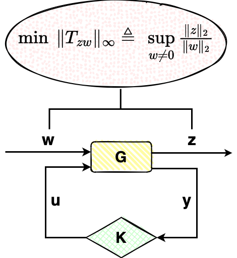
Figure 2: Illustration of the classic $H_{\infty}$ control theory.

Classic $H_{\infty}$ control [42] deals with a system involved with disturbance as shown in Fig. 2, where $G$ is the plant, $K$ is the controller, $u$ is the control input, $y$ is the measurement available to the controller, $w$ is an unknown disturbance, and $z$ is the error output which is expected to be minimized. In general, we wish the controller to stabilize the closed-loop system based on a model of the plant $G$. The goal of $H_{\infty}$ control is to design a controller $K$ that minimize the error $z$ while minimizing the $H_{\infty}$ norm of the closed-loop transfer function $T_{zw}$ from the disturbance $w$ to the error $z$:

$$\|T_{zw}\|_{\infty}=\sup_{w\neq 0}\frac{\|z\|_{2}}{\|w\|_{2}}.$$ (1)

However, minimizing $\|T_{zw}\|_{\infty}$ is usually challenging, in practical implementation, we instead wish to find an acceptable ${\color[rgb]{0,0,0}}>0$ and a controller $K$ satisfying $\|T_{zw}\|_{\infty}<{\color[rgb]{0,0,0}}$, which is called suboptimal $H_{\infty}$ control, we will denote this as ${\color[rgb]{0,0,0}}$-optimal in this paper. According to Morimoto and Doya [21], if $\|T_{zw}\|_{\infty}<{\color[rgb]{0,0,0}}$, it is guaranteed that the system will remain stabilized for any disturbance mapping $\mathbf{d}:z\mapsto w$ with $\|\mathbf{d}\|_{\infty}<\frac{1}{{\color[rgb]{0,0,0}}}$.

Finding a ${\color[rgb]{0,0,0}}$-optimal $H_{\infty}$ controller is modeled as a Min-Max problem, considering the plant $G$ with dynamics given by

$$\dot{\mathbf{x}}=f(\mathbf{x},\mathbf{u},\mathbf{w}),$$ (2)

where $\mathbf{x}\in X\subset\mathbf{R}^{n}$ is the state, $\mathbf{u}\in U\subset\mathbf{R}^{m}$ is the control input, and $\mathbf{w}\in W\subset\mathbf{R}^{l}$ is the disturbance input.

The $H^{\infty}$ control problem can be considered as the problem of finding a controller that satisfies a constraint

$$\left\|T_{zw}\right\|_{\infty}^{2}=\sup_{\mathbf{w}}\frac{\|\mathbf{z}\|_{2}{}^{2}}{\|\mathbf{w}\|_{2}{}^{2}}<{\color[rgb]{0,0,0}}^{2},$$ (3)

where $\mathbf{z}$ is the error output. In other words, because the norm $\|\mathbf{z}\|_{2}$ and the norm $\|\mathbf{w}\|_{2}$ are defined as

$$\|\mathbf{z}\|_{2}^{2} =\int_{0}^{\infty}\mathbf{z}^{T}(t)\mathbf{z}(t)dt$$ (4)

$$\|\mathbf{w}\|_{2}^{2} =\int_{0}^{\infty}\mathbf{w}^{T}(t)\mathbf{w}(t)dt,$$

our goal is to find a control input $\mathbf{u}$ satisfying:

$$V=\int_{0}^{\infty}(\mathbf{z}^{T}(t)\mathbf{z}(t)-{\color[rgb]{0,0,0}}^{2}\mathbf{w}^{T}(t)\mathbf{w}(t))dt<0,$$ (5)

here $\mathbf{w}$ is any possible disturbance with $x(0)=\mathbf{0}$. By solving the following min-max game, we can find the best control input $\mathbf{u}$ that minimizes $V$ while the worst disturbance $\mathbf{w}$ is chosen to maximize $V$:

$$V^{*}=\underset{\mathbf{u}}{\operatorname{min}}\underset{\mathbf{w}}{\operatorname{max}}\int_{0}^{\infty}(\mathbf{z}^{T}(t)\mathbf{z}(t)-{\color[rgb]{0,0,0}}^{2}\mathbf{w}^{T}(t)\mathbf{w}(t))dt<0.$$ (6)

III-B Reinforcement Learning

Reinforcement learning is based upon Markov Decision Process (MDP) model, which is utilized to represent and solve sequential decision-making problems under uncertainty. An MDP could be defined as $\mathcal{M}=\{S,A,T,R,\gamma\}$, where $S$ stands for the set of all states, $A$ for the set of all actions, $T$ for the transition function where $T(s^{\prime}|s,a)$ specifies the probability of reaching state $s^{\prime}$ after performing action $a$ in state $s$, $R$ for the reward function where $R(s,a)$ defines the immediate reward yielded by taking action $a$ in state $s$, and $\gamma$ for the discount factor.

Solving the MDP is equivalent to finding the optimal policy $\pi^{*}$ maximizing the expectation of cumulative reward across trajectories induced by this policy.

$$\pi^{*}\ =\operatorname*{arg\,max}_{\pi}\mathbb{E}_{\pi}[\sum\limits_{t=0}^{\infty}\gamma^{t}R(s_{t},a_{t})]$$

where the $s_{t}$ and $a_{t}$ is derived recursively as below (given prior state distribution $s_{0}\sim\rho$ and $a_{0}\sim\pi(\cdot|s_{0})$):

$$\forall t\in\mathbb{N}^{*},s_{t}\sim T(\cdot|s_{t-1},a_{t-1}),a_{t}\sim\pi(\cdot|s_{t}).$$

Previous policy optimization methods include Policy Gradient [34], Trust-Region approaches [29] and Proximal Policy Optimization (PPO) [30] etc. In this work, we adopt PPO as our policy optimization approach. We first define the value function $V(s)$ of state $s$ which represents the expected cumulative reward achieved by taking policy $\pi$ from state $s$:

$$V(s)=\mathbb{E}_{\pi}[\sum\limits_{t=0}^{\infty}\gamma^{t}R(s_{t},a_{t})|s_{0}=s]$$

The generalized advantage estimator [31] $A(s)$ of a state is derived as below:

$$A(s_{t})=\gamma^{T-t}V(s_{T})+\gamma^{T-t-1}r_{T-1}+\cdots\gamma r_{t+1}+r_{t}-V(s_{t})$$

where $T$ stands for the number of rollouts, $t$ stands for the current time index in $[0,T]$ and $r_{t}$ represents the immediate reward yielded at the time index $t$. Furthermore, we denote $\pi_{old}$ as the policy utilized to perform rollouts and $\pi_{\theta}$ as the current policy with parameters $\theta$. According to Schulman et al. [30], we set the main objective function as below:

$$L^{CLIP}(\theta)=\mathbb{E}_{t}[\min{(q_{t}(\theta)A(s_{t}),\text{clip}(q_{t}(\theta),1-\epsilon,1+\epsilon)A(s_{t}))}]$$

where $q_{t}(\theta)=\frac{\pi(a_{t}|s_{t})}{\pi_{old}(a_{t}|s_{t})}$ and $\epsilon$ is a hyperparameter determining the maximum stride of policy update. Based on that, the final objective function is constructed as:

$$L(\theta)=\mathbb{E}_{t}[L^{CLIP}(\theta)+c_{1}S(\pi_{\theta}(\cdot|s_{t}))-c_{2}L^{VALUE}(\theta)]$$

where $c_{1},c_{2}$ are predefined coefficients, $S$ denotes entropy function and $L^{VALUE}$ stands for the squared error between the current value function and the target value for state $s_{t}$.

IV Learning $H_{\infty}$ Locomotion Control

In this section, we will firstly give the statement of the robust locomotion problem, then give the detailed definition of the problem. After that, we will describe our method in detail and give a practical implementation.

IV-A Problem Statement

In general, disturbance can be considered as external forces applied to the robots. For simplification, we assume that all external forces can be synthesized into a single force applied to the center of mass(CoM). Under this assumption, we wish to obtain a controller that can maintain stable and good command-tracking under disturbances. Previous methods [22] use random external forces in the training process. However, random external forces are not always effective disturbances for robots. Intuitively, the external forces generation should take into account the state of behavior policies to identify a value impairing as much command tracking performance as possible.

Additionally, the disturbances are expected to be proper and within the tolerance of behavior policy. Otherwise, applying strong disturbances at the early learning stage would hinder or even undermine the training. Thus, it is necessary to have a disturbance generation strategy that evolves with the policy training and adjusts according to the behavior policy.

TABLE I: Reward functions for Unitree A1 standing task

Term (∗ indicates $R^{task}$)	Calculation	Scale
linear velocity tracking∗	$exp(-\|v_{xy}-v_{xy}^{cmd}\|^{2}/\sigma_{track})\ r_{ori}$	$1.0$
angular velocity tracking∗	$exp(-\|\omega_{z}-\omega_{z}^{cmd}\|^{2}/\sigma_{track})\ r_{ori}$	$0.5$
joint velocities	$\|\dot{q}\|^{2}$	$-2e^{-4}$
joint accelerations	$\|\ddot{q}\|^{2}$	$-2.5e^{-7}$
action rate	$\|a_{t+1}-a_{t}\|^{2}$	$-0.01$
joint position limits	$\mathds{1}[q\notin(q_{min},q_{max})]$	$-10.0$
joint velocity limits	$\mathds{1}[\dot{q}\notin(\dot{q}_{min},\dot{q}_{max})]$	$-10.0$
torque limits	$\mathds{1}[\tau\notin(\tau_{min},\tau_{max})]$	$-10.0$
collision	$\sum_{j\in P}j^{contact}/|P|$	$-1.0$
extra collision	$\sum_{j\in E_{p}}j^{contact}/|E_{p}|$	$-1.0$
front feet contact	$\mathds{1}[\sum_{f\in[FL,FR]}f^{contact}==0]$	$1.0$
orientation $r_{ori}$	$(0.5*\cos{(v_{f}\cdot\hat{v}^{*})}+0.5)^{2}$	$1.0$
root height	$\min(e^{h},0.55)$	$1.0$

TABLE II: Reward functions for Unitree Aliengo locomotion task

Term (∗ indicates $R^{task}$)	Calculation	Scale
linear velocity tracking∗	$exp(-\|v_{xy}-v_{xy}^{cmd}\|^{2}/\sigma_{track})$	$1.0$
angular velocity tracking∗	$exp(-\|\omega_{z}-\omega_{z}^{cmd}\|^{2}/\sigma_{track})$	$0.5$
$z$-axis linear velocity	$v_{z}^{2}$	$-2.0$
roll-pitch angular velocity	$\|\omega_{xy}\|^{2}$	$-0.05$
joint power	$\sum|\tau|\odot|\dot{q}|$	$-2e^{-5}$
joint power distribution	$\mathrm{Var}[|\tau|\odot|\dot{q}|]$	$-1e^{-5}$
joint accelerations	$\|\ddot{q}\|^{2}$	$-2.5e^{-7}$
action rate	$\|a_{t}-a_{t-1}\|^{2}$	$-0.01$
smoothness	$\|a_{t}-2a_{t-1}+a_{t-2}\|^{2}$	$-0.01$
joint position limits	$\mathds{1}[q\notin(q_{min},q_{max})]$	$-5.0$
joint velocity limits	$\mathds{1}[\dot{q}\notin(\dot{q}_{min},\dot{q}_{max})]$	$-5.0$
torque limits	$\mathds{1}[\tau\notin(\tau_{min},\tau_{max})]$	$-5.0$
orientation	$\|g_{xy}\|^{2}$	$-0.2$
base height	$\|h-h^{target}\|^{2}$	$-1.0$

IV-B Problem Definition

As described in the former part, we wish to add more effective disturbances, therefore, we model it as a one-step decision problem. Let the disturbance policy or disturber be a function $\mathbf{d}:\mathbf{S}\to\mathbf{D}\subset\mathbf{R}^{3}$, which maps observations to forces. Let $\mathbf{C}:\mathbf{S}\times\mathbf{A}\times\mathbf{D}\to\mathbf{R}^{+}$ be a cost function that measures the errors from commands, expected orientation and base height in the next time-step after an action from some state. Additionally, $\mathbf{C}_{\mathbf{\pi}}^{\mathbf{d}}(s)\equiv\mathbb{E}_{(a,d)\sim(\pi(s),\mathbf{d}(s))}\mathbf{C}(s,a,d)$ denotes the gap between expected performance and actual performance given policy $\mathbf{\pi}$ and disturber $\mathbf{d}$. With these definitions, under $H_{\infty}$ control, we wish to find a policy $\pi$ which stabilizes the system, i.e.

$$\lim_{T\to\infty}\sum\limits_{t=0}^{T}\mathbb{E}_{s_{t}}({\mathbf{C}_{\pi}^{\mathbf{d}}(s_{t})-{\color[rgb]{0,0,0}}^{*}\|\mathbf{d}(s_{t})\|_{2}})<0,$$ (7)

where ${\color[rgb]{0,0,0}}^{*}$ is the optimal value of:

$$\|T(\mathbf{\pi})\|_{\infty}=\sup_{\mathbf{d}\neq 0}\frac{\sum_{t=0}^{\infty}\mathbb{E}_{s_{t}}\mathbf{C}_{\pi}^{\mathbf{d}}(s_{t})}{\sum_{t=0}^{\infty}\mathbb{E}_{s_{t}}\|\mathbf{d}(s)\|_{2}}.$$ (8)

However, this problem is hard to solve. We alternatively solve the sub-optimal problem: for a given ${\color[rgb]{0,0,0}}>0$, we wish to find an admissible policy $\pi$ such that

$$\lim_{T\to\infty}\sum\limits_{t=0}^{T}\mathbb{E}_{s_{t}}({\mathbf{C}_{\pi}^{\mathbf{d}}(s_{t})-{\color[rgb]{0,0,0}}\|\mathbf{d}(s_{t})\|_{2}})<0,$$ (9)

We say that a policy $\pi$ satisfying the above condition is ${\color[rgb]{0,0,0}}$-optimal. More intuitively, if a policy is ${\color[rgb]{0,0,0}}$-optimal, then an external force $f$ can get a performance decay at most ${\color[rgb]{0,0,0}}\|f\|_{2}$. Additionally, we wish the disturbances to be effective, which means that it can maximize the cost of policy with limited intensity. Therefore, for a policy $\pi$, and a discount factor $0\leq\gamma_{2}<1$, the target of $\mathbf{d}$ is to maximize:

$$\mathbb{E}_{\mathbf{d}}[\sum\limits_{t=0}^{\infty}\gamma_{2}^{t}(\mathbf{C}_{\pi}^{\mathbf{d}}(s_{t})-{\color[rgb]{0,0,0}}\|\mathbf{d}(s_{t})\|_{2})]$$ (10)

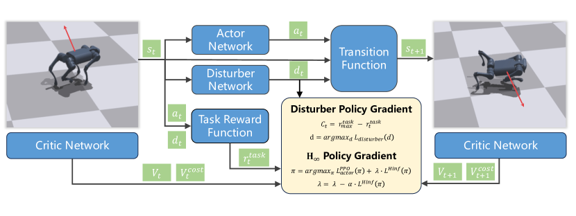
Figure 3: Overview of $H_{\infty}$ locomotion control method. The blue box indicates a trainable module, the light yellow box is the loss function to optimize these modules, and the green box indicates the data collected for training. At every time step during the training process, the current observation is fed into both the actor and disturber. We perform a simulation step based on the robot’s action and the external force generated by the disturber. The current task reward is derived based upon transition, and our double-head critic outputs estimation for both task value and also overall value. During the optimization process, we perform policy gradient on the disturber to learn proper forces based on the current performance of behavior policy, and carry out $H_{\infty}$ policy gradient by optimizing the PPO loss of the actor while taking into consideration the novel constraint $L^{H_{inf}}$ which we introduce to stabilize the training procedure. We adopt a dual gradient descent approach to address this constrained policy optimization problem.

IV-C MDP Formulation of the Problem

With the definition of the problem in IV-B, we give a MDP formulation of the problem in this section. First, we give a fundamental MDP of the control and disturbance process, $\mathcal{M}=\{S,A\times D,T,R^{*},\gamma\}$, here $S$ stands for the set of all states, $A$ for the set of all actions, $D$ for the set of all disturbances, $R^{*}$ for the reward function where $R^{*}(s,a,d)$ defines the immediate reward yielded by taking action $a$ in state $s$ for policy $T(s^{\prime}|s,a,d)$ specifies the probability of reaching state $s^{\prime}$ after performing action $a$ and disturbance $d$ in state $s$, $\gamma$ for the discount factor. However, it is hard to solve this MDP without proper reward function $R^{*}$. Therefore, we formulate the problem by dividing it into two related MDPs which are expected to be solved by policy and disturber respectively.

The MDPs that are expected to be solved by policy and disturber can be written as $\mathcal{M}_{1}=\{S,A,T_{1},R_{1},\gamma_{1}\}$ and $\mathcal{M}_{2}=\{S,D,T_{2},R_{2},\gamma_{2}\}$ respectively. Here $R_{1}$ for the reward function where $R_{1}(s,a)=\mathbb{E}_{d\sim\mathbf{d}(s)}R(s,a,d)$ defines the immediate reward yielded by taking action $a$ in state $s$ for policy, $R_{2}(s,d)=\mathbb{E}_{a\sim\mathbf{\pi}(s)}\mathbf{C}(s,a,d)-\eta\|d\|_{2}$ defines the immediate reward yielded by taking disturbance $d$ in state $s$ for disturber, $\gamma_{1}$ for the discount factor of policy and $\gamma_{2}$ for discount factor of disturber. $T_{1}$ for the transition function where $T_{1}(s^{\prime}|s,a)$ specifies the probability of reaching state $s^{\prime}$ after performing action $a$ in state $s$, $T_{2}$ for the transition function where $T_{2}(s^{\prime}|s,d)$ specifies the probability of reaching state $s^{\prime}$ after performing action $d$ in state $s$. With $\mathcal{M}$, it is easy to get the relation of of $\mathcal{M}_{1}$ and $\mathcal{M}_{2}$, which is described as $T_{1}(s^{\prime}|s,a)=T(s^{\prime}|s,a,\mathbf{d}(s))$ and $T_{2}(s^{\prime}|s,d)=T(s^{\prime}|s,\pi(s),d)$, where $\pi$ is the policy and $\mathbf{d}$ is the disturber. It is notable that we expect the disturbance MDP $\mathcal{M}_{2}$ to lay more emphasis on short-term returns, so we designate $\gamma_{2}=0.8$ in our problem.

IV-D Method

In reinforcement learning-based locomotion control, the reward functions are usually complicated [19, 41, 9, 22], some of them guide the policy to complete the task, and some of them act as regularization to the policy. In our work, we divide the reward functions into two categories, the task rewards and the auxiliary rewards, the former part leads the policy to achieve command tracking and maintain good orientation and base height, and the latter part leads the policy to satisfy the physical constraints of robot and give smoother control. We present the details of our reward functions in Table I and II. To clarify the meaning of some symbols used in the reward functions, $P$ denotes the set of all joints whose collisions with the ground are penalized, and $E_{p}$ denotes the set of joints with stronger penalization. $f^{contact}$ stands for whether foot $f$ has contact with the ground. Moreover, $g$ denotes the projection of gravity onto the local frame of the robot, and $h$ denotes the base height of the robot. In the standing task particularly, we define an ideal orientation $v^{*}$ for the robot base, which we assign the value $v^{*}=(0.2,0.0,1.0)$, and accordingly define the unit ideal orientation $\hat{v}^{*}=\frac{v^{*}}{\|v^{*}\|}$. We expect the local $x-$axis of the robot, which we denote as $v_{f}$, to be aligned to $\hat{v}^{*}$, and thus adopt cosine similarity as a metric for the orientation reward. Besides, we scale the tracking rewards by the orientation reward $r_{ori}$ in the standing task because we expect the robot to stabilize itself in a standing pose before going on to follow tracking commands.

Now we denote the rewards from each part as task rewards $R^{task}$ and auxiliary rewards $R^{aux}$ respectively, and the overall reward as $R$. Firstly, we assume that the task reward has an upper bound $R^{task}_{max}$, then the cost can be formulated as $\mathbf{C}=R^{task}_{max}-R^{task}$. With $R$ and $C$, we can get value functions for overall reward and cost, denoted as $V$ and $V^{cost}$. Then the goal of the actor is to solve:

$$\begin{array}[]{ll}\underset{\pi}{\operatorname{maximize}}&\mathbb{E}_{t}\left[\frac{\pi\left(a_{t}\mid s_{t}\right)}{\pi_{\text{old }}\left(a_{t}\mid s_{t}\right)}A(s_{t})\right]\\ \text{ subject to }&\mathbb{E}_{t}\left[\operatorname{KL}\left[\pi_{\text{old }}\left(\cdot\mid s_{t}\right),\pi\left(\cdot\mid s_{t}\right)\right]\right]\leq\delta\\ &\mathbb{E}_{t}\left[{\color[rgb]{0,0,0}}\|\mathbf{d}(s_{t})\|_{2}-\mathbf{C_{\pi}}(s_{t})\right]>0,\end{array}$$ (11)

where $A$ is the advantage with respect to overall reward, and the goal of the disturber is to solve:

$$\begin{array}[]{ll}\underset{\mathbf{d}}{\operatorname{maximize}}&\mathbb{E}_{t}\left[\frac{\mathbf{d}\left(d_{t}\mid s_{t}\right)}{\mathbf{d}_{\text{old }}\left(d_{t}\mid s_{t}\right)}(\mathbf{C_{\pi}}(s_{t})-{\color[rgb]{0,0,0}}\|\mathbf{d}(s_{t})\|_{2})\right]\\ \text{ subject to }&\mathbb{E}_{t}\left[\operatorname{KL}\left[\mathbf{d}_{\text{old }}\left(\cdot\mid s_{t}\right),\mathbf{d}\left(\cdot\mid s_{t}\right)\right]\right]\leq\delta.\end{array}$$ (12)

However, asking a high-frequency controller to be strictly robust in every time step is unpractical, so we replace the constraint $\mathbb{E}_{t}\left[{\color[rgb]{0,0,0}}\|\mathbf{d}(s_{t})\|_{2}-\mathbf{C_{\pi}}(s_{t})\right]>0$ with a more flexible substitute:

$$\mathbb{E}_{t}\left[{\color[rgb]{0,0,0}}\|\mathbf{d}(s_{t})\|_{2}-\mathbf{C_{\pi}}(s_{t})+{\color[rgb]{0,0,0}{V^{cost}(s_{t})-V^{cost}(s_{t+1})}}\right]>0,$$ (13)

where $V^{cost}$ is the value function of the disturber with respect to $\mathcal{M}_{2}$ defined in IV-C. Intuitively, if the policy guides the robot to a better state, the constraint will be slackened, otherwise the constraint will be tightened. We will show that using this constraint, the actor is also guaranteed to be ${\color[rgb]{0,0,0}}$-optimal.

We follow PPO to deal with the KL divergence part and use the dual gradient decent method [25] to deal with the extra constraint, denoted as $L^{Hinf}(\pi)\triangleq\mathbb{E}_{t}[{\color[rgb]{0,0,0}}\|\mathbf{d}(s_{t})\|_{2}-\mathbf{C_{\pi}}(s_{t})+{\color[rgb]{0,0,0}{V^{cost}(s_{t})-V^{cost}(s_{t+1})}}]>0$, then the update process of policy can be described as:

$$\pi =\underset{\pi}{\operatorname{argmax}}L^{PPO}_{actor}(\pi)+\lambda*L^{Hinf}(\pi)$$ (14)

$$\mathbf{d} =\underset{\mathbf{d}}{\operatorname{argmax}}L_{disturber}(\mathbf{d})$$

$$\lambda =\lambda-\alpha*L^{Hinf}(\pi),$$

where $L^{PPO}_{actor}(\pi)$ is the PPO objective function for the actor, $L_{disturber}(\mathbf{d})$ is the objective function for disturber with a similar form as PPO objective function but replacing the advantage with $\mathbf{C_{\pi}}(s)-{\color[rgb]{0,0,0}}\|\mathbf{d}(s)\|_{2}$, $\lambda$ is the Lagrangian multiplier of the proposed constraint, and $\alpha$ is the step-size of updating $\lambda$. We present an overview of our method in Fig. 3 and summarized our algorithm in Algorithm 1.

Input: Initial actor $\pi_{0}$, disturber $\mathbf{d}_{0}$, overall value function $V_{0}$, task value function $V_{0}^{cost}$, initial guess ${\color[rgb]{0,0,0}}_{0}$, initial multiplier $\beta_{0}$, upper bound of task reward $R_{max}^{cost}$

Output: policy $\pi$, disturber $\mathbf{d}$

$\pi_{old}=\pi_{0}$, $\mathbf{d}_{old}=\mathbf{d}_{0}$, $V_{old}=V_{0}$, $V_{old}^{cost}=V_{0}^{cost}$

for iteration = $1,2,\cdots,\text{max iteration}$ do

       Run policy $\pi_{old}$ in environment for $T$ time steps

       Compute values of each states with $V_{old}$

       Compute cost values of each states with $V_{old}^{cost}$

       Compute costs $C_{t}=R_{max}^{task}-R_{t}$

       Compute advantage estimation $A_{t}$

       Optimize $\pi$ with $L^{PPO}_{actor}+\lambda*L^{Hinf}$

       Optimize $\mathbf{d}$ with $L_{disturber}$

       $\lambda=\lambda-\alpha*L^{Hinf}$

       ${\color[rgb]{0,0,0}}=0.9*{\color[rgb]{0,0,0}}+0.1*\frac{\sum_{t=1}^{T}C_{t}}{\sum_{t=1}^{T}\|\mathbf{d}_{old}\|_{2}}$

       $\pi_{old}=\pi$

       $\mathbf{d}_{old}=\mathbf{d}$

end for

Algorithm 1 Learning $H_{\infty}$ Locomotion Control

(a) Slopes

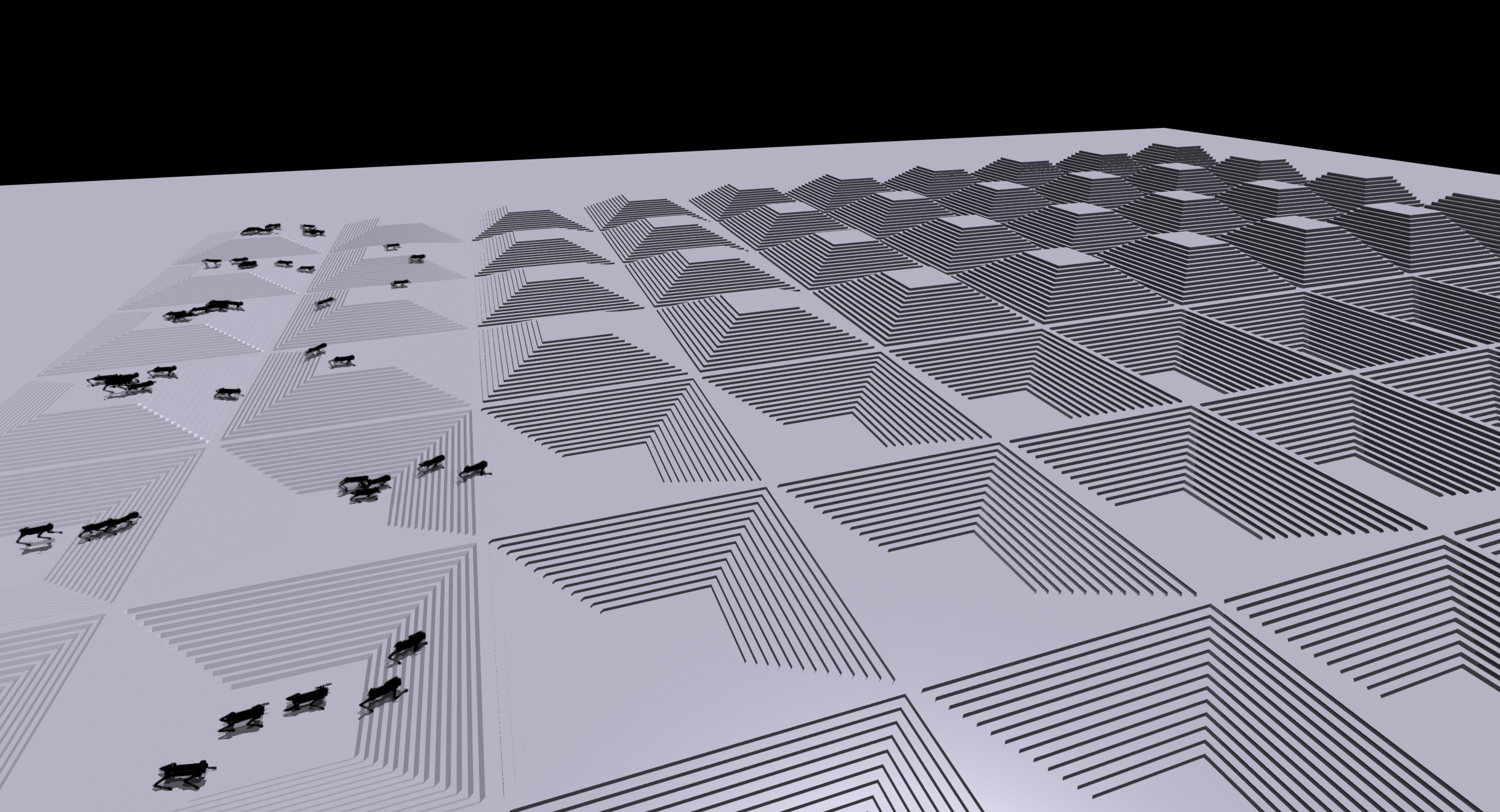
(b) Stairs

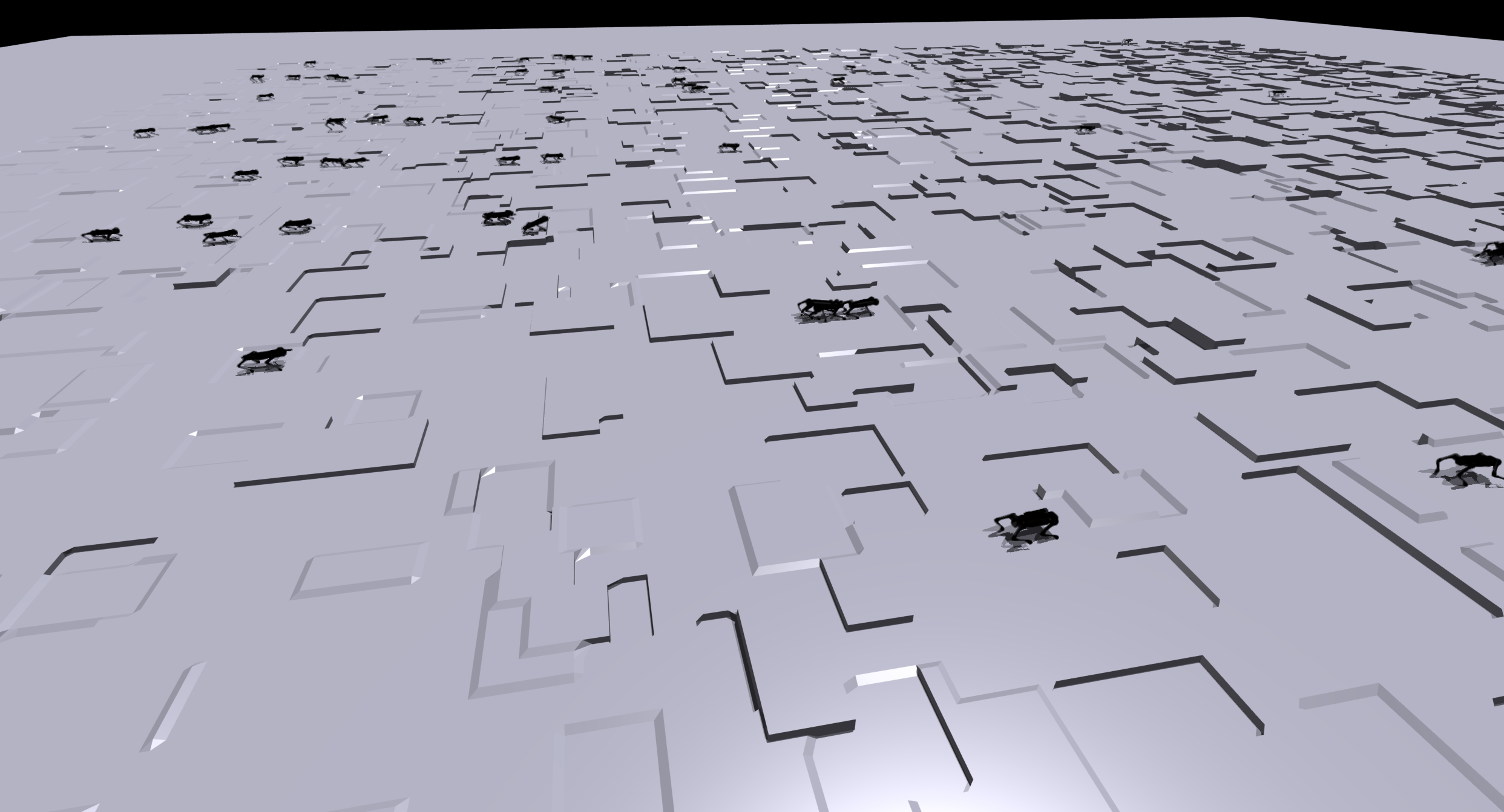
(c) Discrete height fields

Figure 4: Demonstration of different terrains used in simulated training environments

IV-E ${\color[rgb]{0,0,0}}$-optimality

We assume that $0\leq\mathbf{C}(s,a)\leq C_{max}$ where $C_{max}<\infty$ is a constant. We also assume that there exists a value function $V_{\pi}^{cost}$ such that $0\leq V_{\pi}^{cost}(s)\leq V_{max}^{cost}$ for any $s\in\mathbf{S}$, where $V_{max}^{cost}<\infty$. Besides, we denote $\beta_{\pi}^{t}(s)=P(s_{t}=s|s_{0},\pi)$, where $s_{0}$ is sampled from initial states, and assume that the the stationary distribution of the Markov chain under policy $\pi$ is $\beta_{\pi}(s)=\lim_{t\to\infty}\beta_{\pi}^{t}(s)$ exists. All the assumptions are normal in reinforcement learning, then we have the following theorem:

Theorem 1.

If $\mathbf{C}_{\pi}(s)-{\color[rgb]{0,0,0}}\|\mathbf{d}(s)\|_{2}<\mathbb{E}_{s^{\prime}\sim P(\cdot|\pi,s)}({\color[rgb]{0,0,0}{V_{\pi}^{cost}(s)-V_{\pi}^{cost}(s^{\prime})}})$ for $s\in\mathbf{S}$ with $\beta_{\pi}(s)>0$, the policy $\pi$ is ${\color[rgb]{0,0,0}}$-optimal.

proof:

$$\lim_{T\to\infty}\frac{1}{T}\sum_{t=0}^{T}\mathbb{E}_{s_{t}}({\mathbf{C}_{\pi}(s_{t})-{\color[rgb]{0,0,0}}\|\mathbf{d}(s_{t})\|_{2}})$$

$$< \lim_{T\to\infty}\frac{1}{T}\sum_{t=0}^{T}\mathbb{E}_{s_{t}}(\mathbb{E}_{s_{t+1}\sim P(\cdot|\pi,s_{t})}({\color[rgb]{0,0,0}{V_{\pi}^{cost}(s_{t})-V_{\pi}^{cost}(s_{t+1})}}))$$

$$= \lim_{T\to\infty}\frac{1}{T}\sum_{t=0}^{T}\int_{\mathbf{S}}\beta_{\pi}^{t}(s_{t})$$

$$\int_{\mathbf{S}}P(s_{t+1}|s_{t},\pi)({\color[rgb]{0,0,0}{V_{\pi}^{cost}(s_{t})-V_{\pi}^{cost}(s_{t+1})}})ds_{t+1}ds_{t}$$

$$= \lim_{T\to\infty}\frac{1}{T}\sum_{t=0}^{T}\int_{\mathbf{S}}\beta_{\pi}^{t}(s_{t}){\color[rgb]{0,0,0}{V_{\pi}^{cost}(s_{t})}}ds_{t}$$

$$- \int_{\mathbf{S}}\beta_{\pi}^{t}(s_{t})\int_{\mathbf{S}}P(s_{t+1}|s_{t},\pi){\color[rgb]{0,0,0}{V_{\pi}^{cost}(s_{t+1})}}ds_{t+1}ds_{t}$$

$$= \lim_{T\to\infty}\frac{1}{T}\sum_{t=0}^{T}(\mathbb{E}_{s_{t}}{\color[rgb]{0,0,0}{V_{\pi}^{cost}(s_{t})}}$$

$$- \int_{\mathbf{S}}\int_{\mathbf{S}}\beta_{\pi}^{t}(s_{t})P(s_{t+1}|s_{t},\pi)ds_{t}{\color[rgb]{0,0,0}{V_{\pi}^{cost}(s_{t+1})}}ds_{t+1})$$

$$= \lim_{T\to\infty}\frac{1}{T}\sum_{t=0}^{T}(\mathbb{E}_{s_{t}}{\color[rgb]{0,0,0}{V_{\pi}^{cost}(s_{t})}}-\mathbb{E}_{s_{t+1}}{\color[rgb]{0,0,0}{V_{\pi}^{cost}(s_{t+1})}})$$

$$= \lim_{T\to\infty}\frac{1}{T}(\mathbb{E}_{s_{0}}{\color[rgb]{0,0,0}{V_{\pi}^{cost}(s_{0})}}-\mathbb{E}_{s_{T+1}}{\color[rgb]{0,0,0}{V_{\pi}^{cost}(s_{T+1})}})$$

$$\leq \lim_{T\to\infty}\frac{1}{T}({\color[rgb]{0,0,0}{V_{max}^{cost}}}-0)=0$$

Therefore we get $\lim\limits_{T\to\infty}\frac{1}{T}\sum\limits_{t=0}^{T}\mathbb{E}_{s_{t}}({\mathbf{C}_{\pi}(s_{t})-{\color[rgb]{0,0,0}}\|\mathbf{d}(s_{t})\|_{2}})<0$, and $\lim\limits_{T\to\infty}\sum\limits_{t=0}^{T}\mathbb{E}_{s_{t}}({\mathbf{C}_{\pi}(s_{t})-{\color[rgb]{0,0,0}}\|\mathbf{d}(s_{t})\|_{2}})<0$ follows directly.

V Experimental Results

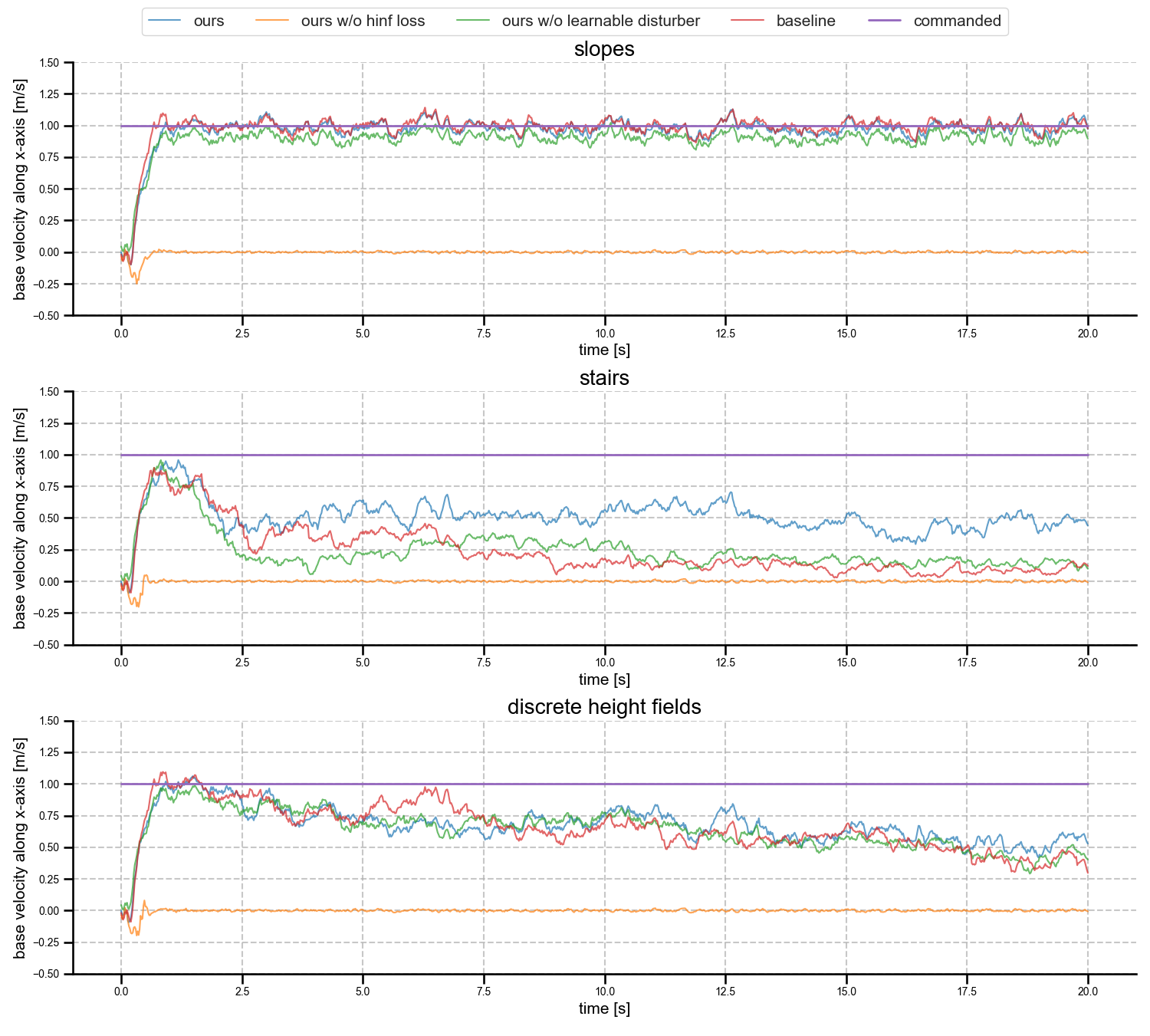
Figure 5: We tested the tracking curve of our method and baselines under continuous random forces.

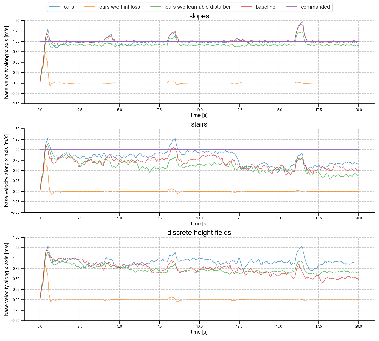
Figure 6: We tested the tracking curve of our method and baselines under sudden large forces.

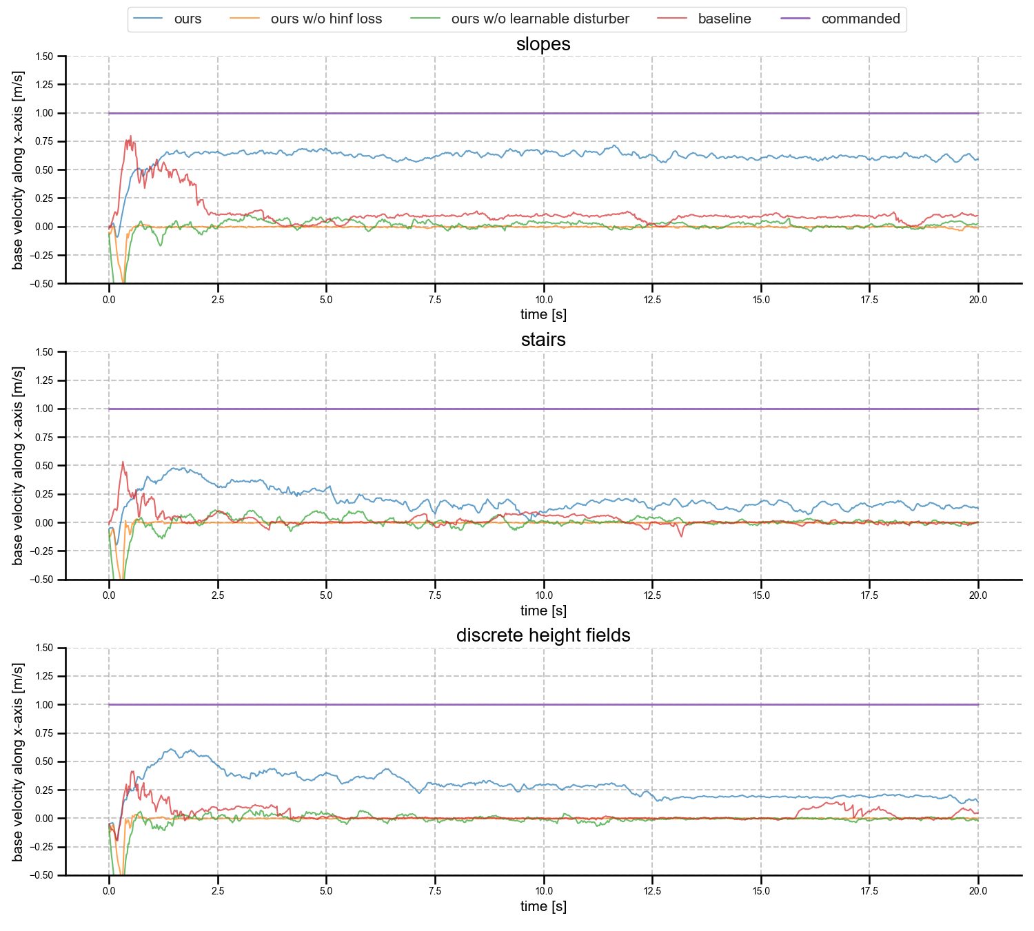
Figure 7: We tested the tracking curve of our method and baselines with disturbers trained to attack specific policy.

(a) stair traversal with forces on legs

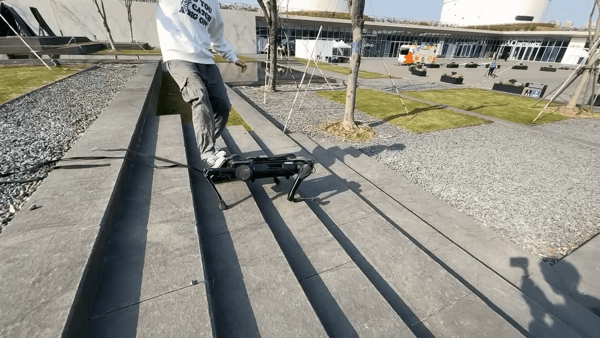
(b) stair traversal under arbitrary kicking

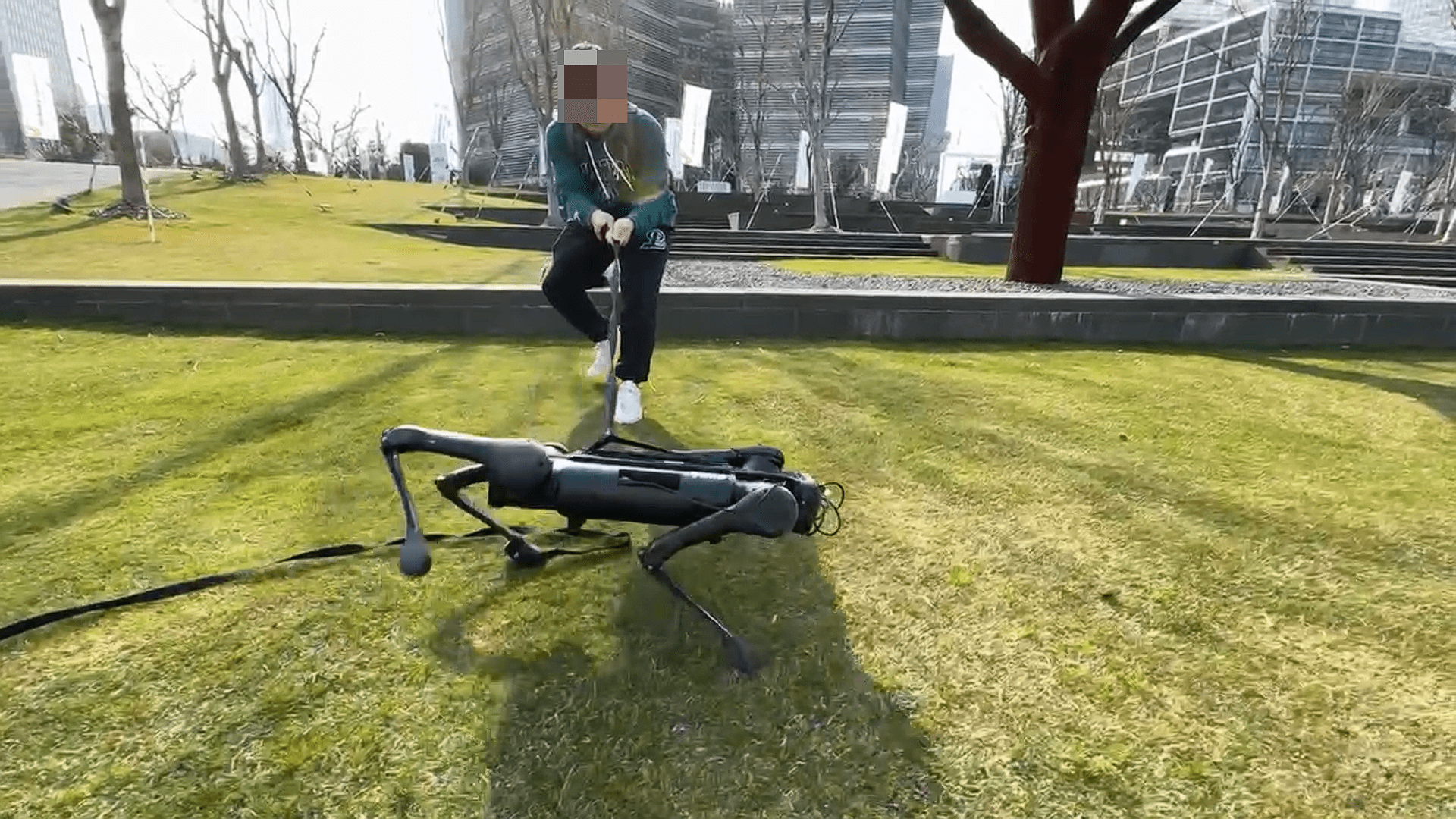
(c) sprinting with forces on trunk

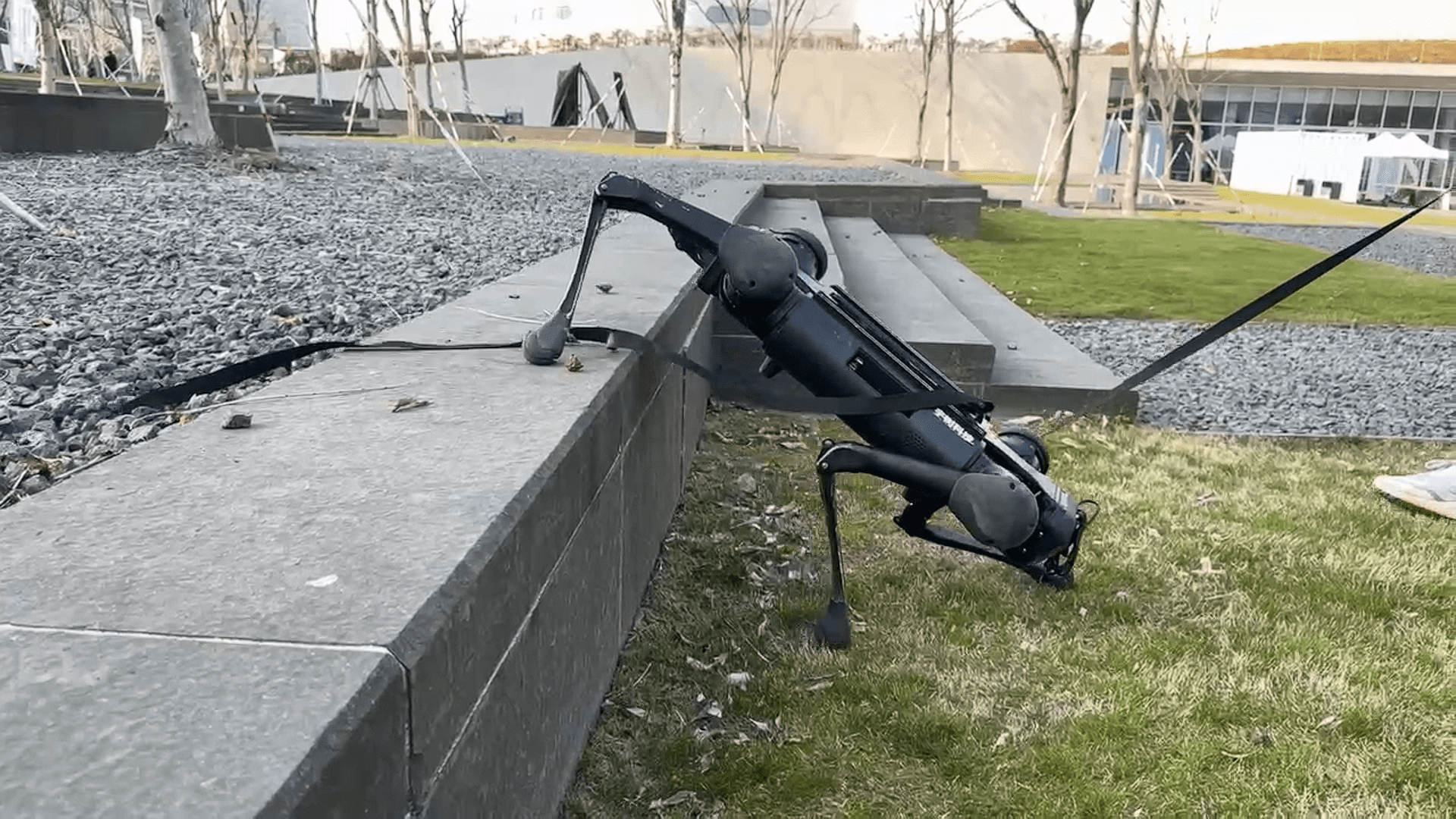
(d) jumping from high platform under pulling

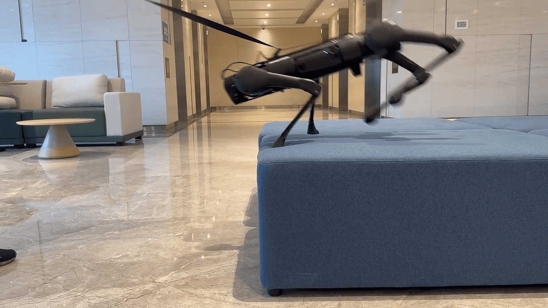
(e) jumping from deformable high platform under disturbances

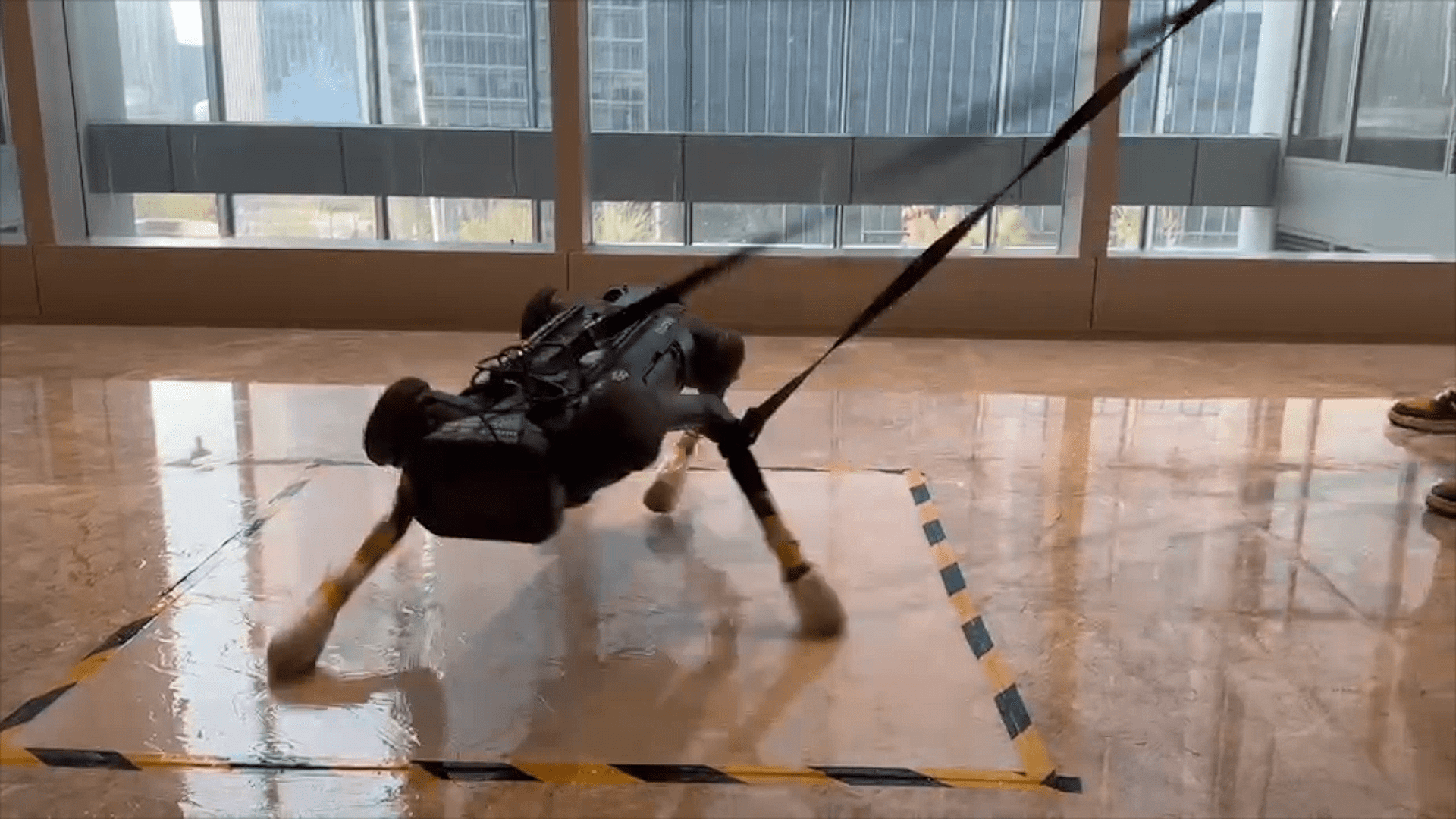
(f) walking over slippery surface with random pulling

(g) slope traversal with forces on trunk

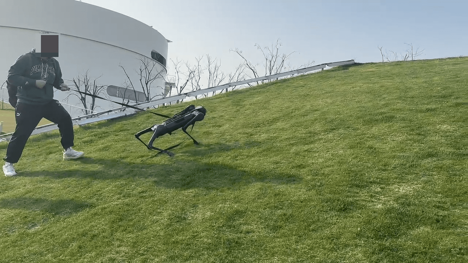
(h) slope traversal with forces on legs

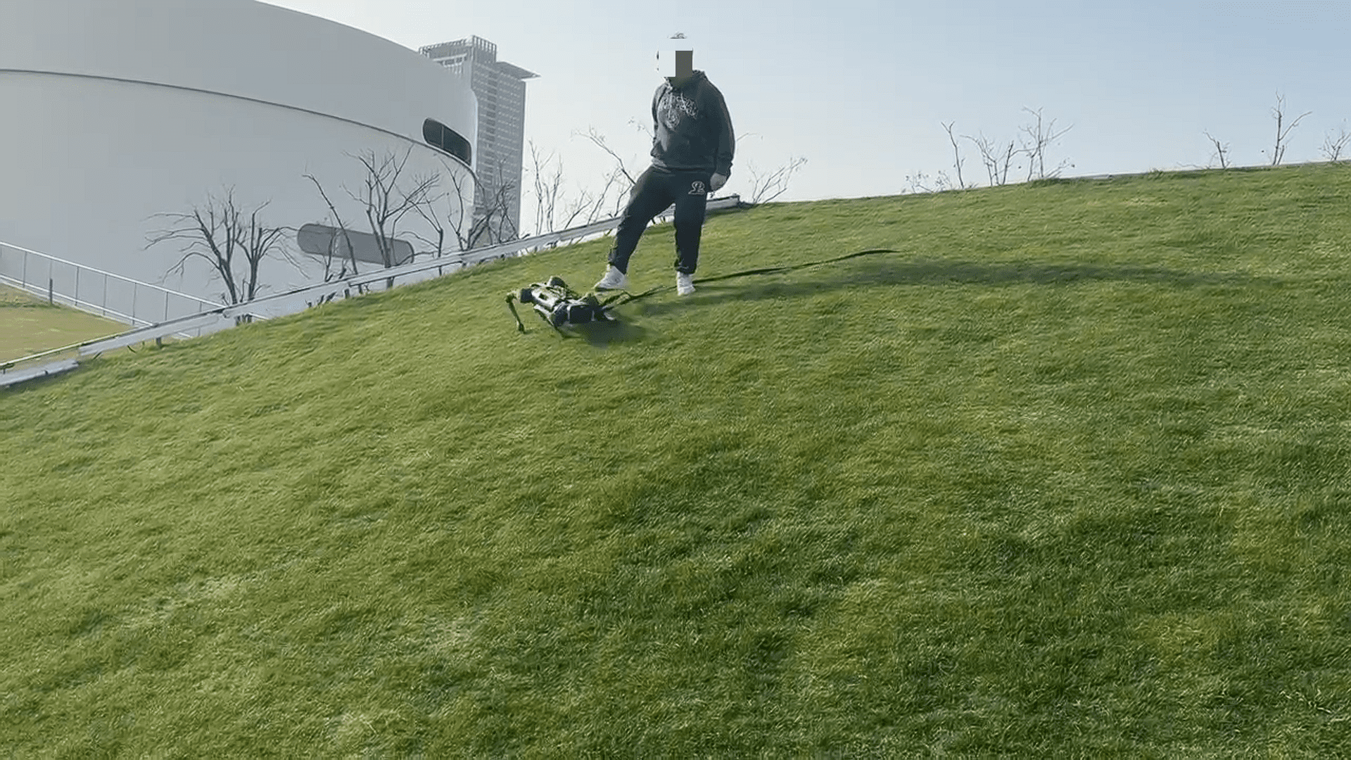
(i) slope traversal under arbitrary kicking

Figure 8: Demonstrations of our method deployed on Unitree Aliengo quadruped robot in real-world settings, with a wide variety of terrains, velocity commands and disturbances.

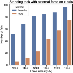
(a) $x-$axis failure case count

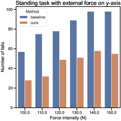
(b) $y-$axis failure case count

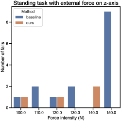
(c) $z-$axis failure case count

Figure 9: Comparison between our method and baseline model on the number of falls under different external forces

In this section, we conduct experiments to show the effectiveness of our method. We implemented the most recent method for non-vision quadrupedal locomotion control [16] as our baseline to solve the same task with the involvement of stochastic disturbances. We then demonstrate how these tasks can be solved better with our method. Our experiments aim to answer the following concrete questions:

• Can our method handle continuous disturbances as well as the current RL method?

• Can current RL methods handle the challenges of sudden extreme disturbances?

• Can current RL methods withstand deliberate disturbances that intentionally attack the controller?

• Can our method be deployed to real robots?

• Is our method applicable to other tasks that require stronger robustness?

To reflect the effectiveness of the novel H-infinity loss and the disturber network, we design four different training settings for comparison studies. First, we train a policy in complete settings where both H-infinity loss and a disturber network are exploited, which we refer to as ours. We clip the external forces to have an intensity of no more than 100N for sake of robot capability. Next, we remove the H-infinity loss from the training pipeline and obtain another policy, which we refer to as ours without hinf loss. Then, we remove the disturber network from ours and replace it with a disturbance curriculum whose largest intensity grows linearly from 0N to 100N with the training process (reaches 100N at the 2000th iteration) and whose direction is sampled uniformly. We call the policy derived from this training procedure ours without learnable disturber. Finally, we train a vanilla policy without both H-infinity loss and disturber network, which also experiences random external forces with curriculum disturbance as described above. We refer to this policy as the baseline. Note that all the four policies are trained on the same set of terrains, including plane, rough slopes, stairs, and discrete height fields. The demonstration of the three non-flat terrains can be found in Fig. 4.

We use Isaac Gym [18, 28] with 4096 parallel environments and a rollout length of 100 time steps. Our training platform is RTX 3090. We randomize the ground friction and restitution coefficients, the motor strength, the joint-level PD gains, the system delay and the initial joint positions in each episode. The randomization ranges for each parameter are detailed in Table III.

TABLE III: Domain Randomizations and their Respective Range

Parameters	Range[Min, Max]	Unit
Ground Friction	$[0.2,2.75]$	-
Ground Restitution	$[0.0,1.0]$	-
Joint $K_{p}$	$[0.8,1.2]\times 20$	-
Joint $K_{d}$	$[0.8,1.2]\times 0.5$	-
Initial Joint Positions	$[0.5,1.5]\times$ nominal value	$\mathrm{rad}$

The training process for all policies lasts 5000 epochs. The real-world experimental results are available in the supplementary materials.

V-A Can our method handle continuous disturbances as well as the baseline method?

To answer question 1, we exploit the four policies mentioned above and apply random continuous disturbances which are drawn from a uniform distribution ranging from 0-100N with the same frequency as controllers. We carry out the experiments in three different kinds of simulated environments: rough slopes, staircases, and discrete height fields. We commanded the robot to move forward with a velocity of 1.0 m/s. The tracking curves in Fig. 5 show that our method has the same capability of dealing with continuous disturbances on rough slopes and discrete height fields as baseline methods, and that our method even performs better on staircases under the disturbances that baseline methods may have already experienced during their training process. On all these terrains, the policy trained without H-infinity loss fails immediately, which again provides evidence that vanilla adversarial training is likely to fail in the field of robot locomotion. In an overall sense, our method can achieve better performance under continuous disturbances, even if the baseline methods have already experienced these disturbances during their training process.

V-B Can current RL methods handle the challenges of sudden extreme disturbances?

To answer question 2, we exploit the four policies mentioned in Sec.V, and apply sudden large external forces on the trunk of robots. We apply identical forces to all robots with an intensity of 150N and a random direction sampled uniformly. The external forces are applied every 4 seconds and last 0.5 seconds. We carry out the experiments in three different kinds of simulated environments: rough slopes, staircases and discrete height fields. In order to compare the robustness of these four policies under extreme disturbances, we give a velocity command which requires the robots to retain a 1.0 m/s velocity along its local x-axis. The tracking curves for the four controllers are shown in Fig. 6. The results indicate that our method achieves greater robustness in every of the three challenging terrains, showcasing better tracking performance. It is noteworthy that the controllers trained without either disturber network or H-infinity loss perform even worse than the baseline, especially the one without H-infinity loss which hardly moves forward. This suggests that in the adversarial training setting, policy and disturber lose balance in lack of H-infinity loss, and justifies our introduction of this novel constraint in pursuit of more stabilized training.

V-C Can current RL methods withstand deliberate disturbances that intentionally attack the controller?

To answer question 3, we fix the four policies mentioned above, and use the disturber training process of our method to train a disturber from scratch for each policy. As a result, each disturber is optimized to discover the weakness of each policy and undermine its performance as much as possible. We perform the disturber training for 500 epochs and examine the tracking performance of the four policies under the trained disturber respectively. We command that the robots move with a velocity of 1m/s along its local x-axis, and carry out comparison studies on three challenging terrains: rough slopes, stairs, and discrete height fields. We illustrate the performance of the four controllers in Fig. 7. The results indicate that our method achieves greater robustness under disruption of deliberate disturbers, with an overall superior performance over the three baselines no matter the terrain types. This suggests that our method has strong robustness against intentional attacks to the controller.

V-D Can our method be deployed to real robots?

To answer question 4, we trained our policy to mature disturbances of up to 100 N of intensity and evaluated our trained policies on Unitree Aliengo quadrupedal robots in the wild. As is shown in Fig. 8, it manages to traverse various terrains such as staircases, high platforms, slopes, and slippery surfaces, withstand disturbances on trunk, legs, and even arbitrary kicking, and handle different tasks such as sprinting. Videos of real-world deployment can be found in supplementary materials.

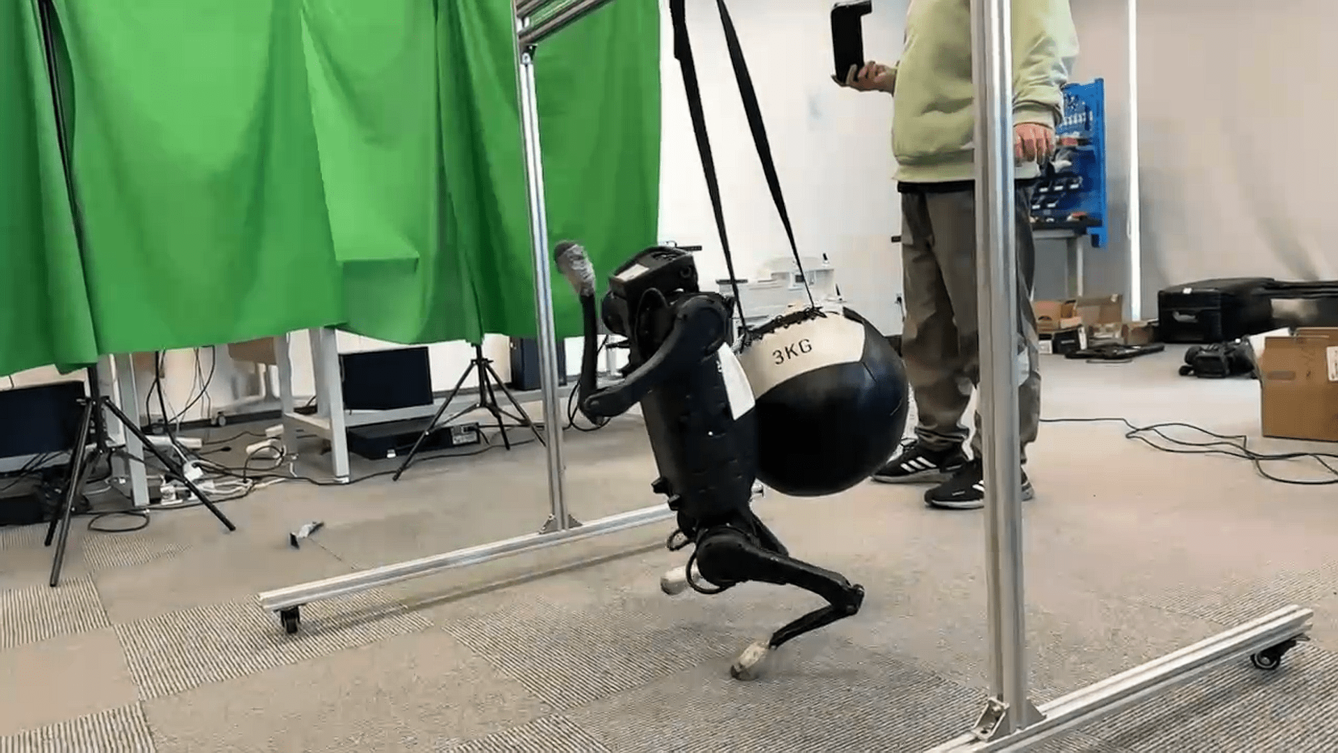
(a) Under collision with a 3kg object

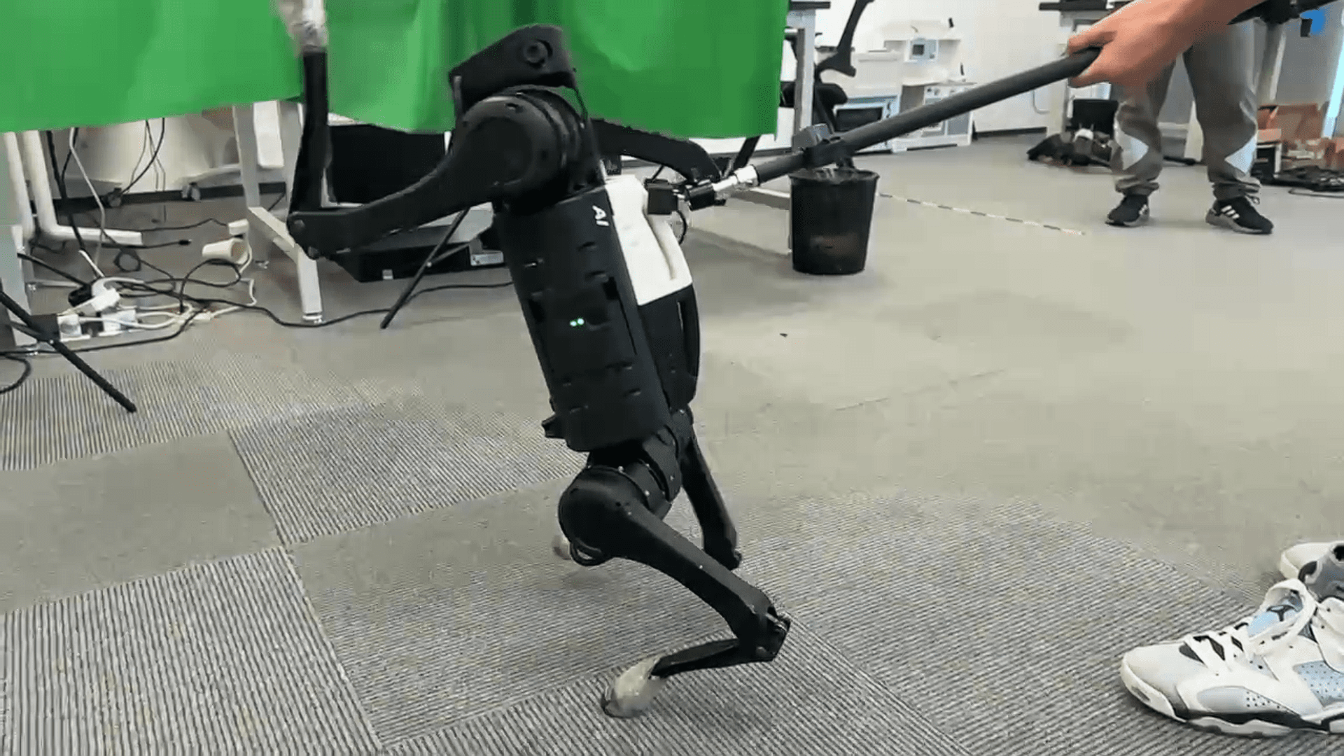
(b) Under random pushing

Figure 10: Demonstrations of our controller performing bipedal standing task under various disturbances.

V-E Is our method applicable to other tasks that require stronger robustness?

To answer question 5, we train the robot to walk with its two rear legs and testify the policy under intermittent exertion of large external forces. We carry out the training process for 10000 epochs because this task is more demanding than locomotion. Similar to the locomotion task, the baseline policy is trained with a normal random disturber while our method is trained with the proposed adaptive disturber. Both disturbers have the same sample space ranging from 0N to 50N. To measure the performance of both methods, we count the total times of falls in one episode when external forces are exerted. Each evaluation episode lasts 20 seconds. Every 5 seconds, the robot receives a large external force with an intensity of 100N that lasts 0.2 seconds. For each method, the evaluation runs 32 times repeatedly and we report the average number of falls.

We carry out three different experiments, exerting the external forces on the direction of $x,y,z$ axes respectively. The experiment results are shown in Fig. 9. Our method comprehensively achieves superior performance over the baseline policy, and only underperforms the baseline when the external forces are exerted on the $z$ axis with a specific intensity of 140 N. We surmise that this is because of the light weight of the A1 robot. The robot might as well float off the ground with a 140 N external force exerted on the vertical axis. On the other hand, it is worth noting that forces generated by the disturber of our pipeline are always lower than 30N throughout the whole training process, while the normal random disturber generates an average of 50N forces by sampling from a fixed distribution. It suggests that it is likely that a disturber producing larger forces underperforms a disturber producing proper forces. To further testify the robustness of our method, we deploy our policy on Unitree A1 robot and test its anti-disturbance capabilities. As is demonstrated in Fig. 10, our controller is able to withstand collisions with heavy objects and random pushes on its body, while retaining a standing posture. Videos for the standing tasks can be found in supplementary materials. Our method thus serves as a promising solution that allows the automatic designing of a proper disturber, enhancing the robustness of quadruped robots.

VI Conclusion

In this work, we propose $H_{\infty}$ learning framework for quadruped locomotion control. Unlike previous works that simply adopt domain randomization approaches, we design a novel training procedure where an actor and a disturber interact in an adversarial manner. To ensure the stability of the entire learning process, we introduce a novel $H_{\infty}$ constraint to policy optimization. Our $H_{\infty}$ constraint guarantees a bound of ratio between the cost to the intensity of external forces, thus ensuring a performance lower bound for the actor in face of external forces with a certain intensity. In this fashion, the disturber can learn to adapt to the current performance of the actor, and the actor can learn to accomplish its tasks with robustness against physical interruptions. We verify that our method achieves notable improvement in robustness in both locomotion and standing tasks, and deploy our method in real-world settings. Our approach enables quadruped robots to tackle external forces with unseen intensities smoothly during deployment, and showcases superior performance over previous methods using domain randomization strategy. Moreover, our method has the potential to be applied to other robotic systems that require robustness to external disturbances, given that there exist proper measurements for external disruptions and the current performance of the controller. We hope that our work will inspire further research on improving the robustness of quadruped robots and even other robotic systems.

References

- Aalipour and Khani [2023] Ali Aalipour and Alireza Khani. Data-driven h-infinity control with a real-time and efficient reinforcement learning algorithm: An application to autonomous mobility-on-demand systems. 2023. doi: 10.48550/ARXIV.2309.08880. URL https://arxiv.org/abs/2309.08880.
- Agarwal et al. [2023] Ananye Agarwal, Ashish Kumar, Jitendra Malik, and Deepak Pathak. Legged locomotion in challenging terrains using egocentric vision. In Conference on Robot Learning (CoRL), pages 403–415. PMLR, 2023.
- Chang et al. [2022] Xu Chang, Zhitong Zhang, Honglei An, Hongxu Ma, and Qing Wei. Learning fast and agile quadrupedal locomotion over complex terrain, 2022.
- Cheng et al. [2023a] Xuxin Cheng, Ashish Kumar, and Deepak Pathak. Legs as manipulator: Pushing quadrupedal agility beyond locomotion, 2023a.
- Cheng et al. [2023b] Xuxin Cheng, Kexin Shi, Ananye Agarwal, and Deepak Pathak. Extreme parkour with legged robots, 2023b.
- Foerster et al. [2018] Jakob Foerster, Gregory Farquhar, Triantafyllos Afouras, Nantas Nardelli, and Shimon Whiteson. Counterfactual multi-agent policy gradients. In Proceedings of the AAAI conference on artificial intelligence, volume 32, 2018.
- Ha et al. [2020] Sehoon Ha, Peng Xu, Zhenyu Tan, Sergey Levine, and Jie Tan. Learning to walk in the real world with minimal human effort, 2020.
- Haarnoja et al. [2019] Tuomas Haarnoja, Sehoon Ha, Aurick Zhou, Jie Tan, George Tucker, and Sergey Levine. Learning to walk via deep reinforcement learning, 2019.
- Hwangbo et al. [2019] Jemin Hwangbo, Joonho Lee, Alexey Dosovitskiy, Dario Bellicoso, Vassilios Tsounis, Vladlen Koltun, and Marco Hutter. Learning agile and dynamic motor skills for legged robots. Science Robotics, 2019.
- Jenelten et al. [2019] Fabian Jenelten, Jemin Hwangbo, Fabian Tresoldi, C. Dario Bellicoso, and Marco Hutter. Dynamic locomotion on slippery ground. IEEE Robotics and Automation Letters, 4(4):4170–4176, 2019. doi: 10.1109/LRA.2019.2931284.
- Kim et al. [2024] Yunho Kim, Hyunsik Oh, Jeonghyun Lee, Jinhyeok Choi, Gwanghyeon Ji, Moonkyu Jung, Donghoon Youm, and Jemin Hwangbo. Not only rewards but also constraints: Applications on legged robot locomotion, 2024.
- Larby and Forni [2022] Daniel Larby and Fulvio Forni. A passivity preserving h-infinity synthesis technique for robot control. In 2022 IEEE 61st Conference on Decision and Control (CDC), pages 1416–1422. IEEE, 2022.
- Lazaridou et al. [2016] Angeliki Lazaridou, Alexander Peysakhovich, and Marco Baroni. Multi-agent cooperation and the emergence of (natural) language. arXiv preprint arXiv:1612.07182, 2016.
- Lee et al. [2020] Joonho Lee, Jemin Hwangbo, Lorenz Wellhausen, Vladlen Koltun, and Marco Hutter. Learning quadrupedal locomotion over challenging terrain. Science robotics, 2020.
- Li et al. [2023] Yunfei Li, Jinhan Li, Wei Fu, and Yi Wu. Learning agile bipedal motions on a quadrupedal robot, 2023.
- Long et al. [2024] Junfeng Long, Zirui Wang, Quanyi Li, Jiawei Gao, Liu Cao, and Jiangmiao Pang. Hybrid internal model: Learning agile legged locomotion with simulated robot response. In International Conference on Learning Representations, 2024.
- Lowe et al. [2017] Ryan Lowe, Yi I Wu, Aviv Tamar, Jean Harb, OpenAI Pieter Abbeel, and Igor Mordatch. Multi-agent actor-critic for mixed cooperative-competitive environments. Advances in neural information processing systems, 30, 2017.
- Makoviychuk et al. [2021] Viktor Makoviychuk, Lukasz Wawrzyniak, Yunrong Guo, Michelle Lu, Kier Storey, Miles Macklin, David Hoeller, Nikita Rudin, Arthur Allshire, Ankur Handa, and Gavriel State. Isaac gym: High performance gpu-based physics simulation for robot learning, 2021.
- Margolis and Agrawal [2023] Gabriel B Margolis and Pulkit Agrawal. Walk these ways: Tuning robot control for generalization with multiplicity of behavior. In Conference on Robot Learning (CoRL), 2023.
- Margolis et al. [2022] Gabriel B Margolis, Ge Yang, Kartik Paigwar, Tao Chen, and Pulkit Agrawal. Rapid locomotion via reinforcement learning. In Robotics: Science and Systems, 2022.
- Morimoto and Doya [2005] Jun Morimoto and Kenji Doya. Robust reinforcement learning. Neural Computation, 17(2):335–359, 2005.
- Nahrendra et al. [2023] I Made Aswin Nahrendra, Byeongho Yu, and Hyun Myung. Dreamwaq: Learning robust quadrupedal locomotion with implicit terrain imagination via deep reinforcement learning. In International Conference on Robotics and Automation (ICRA), pages 5078–5084. IEEE, 2023.
- Paigwar et al. [2020] Kartik Paigwar, Lokesh Krishna, Sashank Tirumala, Naman Khetan, Aditya Sagi, Ashish Joglekar, Shalabh Bhatnagar, Ashitava Ghosal, Bharadwaj Amrutur, and Shishir Kolathaya. Robust quadrupedal locomotion on sloped terrains: A linear policy approach, 2020.
- Panerati et al. [2021] Jacopo Panerati, Hehui Zheng, SiQi Zhou, James Xu, Amanda Prorok, and Angela P Schoellig. Learning to fly—a gym environment with pybullet physics for reinforcement learning of multi-agent quadcopter control. In IEEE/RSJ International Conference on Intelligent Robots and Systems (IROS), 2021.
- Paternain et al. [2022] Santiago Paternain, Miguel Calvo-Fullana, Luiz F. O. Chamon, and Alejandro Ribeiro. Safe policies for reinforcement learning via primal-dual methods, 2022.
- Peng et al. [2018] Xue Bin Peng, Marcin Andrychowicz, Wojciech Zaremba, and Pieter Abbeel. Sim-to-real transfer of robotic control with dynamics randomization. In International Conference on Robotics and Automation (ICRA), pages 3803–3810. IEEE, 2018.
- Reher et al. [2019] Jacob Reher, Wen-Loong Ma, and Aaron D. Ames. Dynamic walking with compliance on a cassie bipedal robot, 2019.
- Rudin et al. [2022] Nikita Rudin, David Hoeller, Philipp Reist, and Marco Hutter. Learning to walk in minutes using massively parallel deep reinforcement learning. In Conference on Robot Learning (CoRL), pages 91–100. PMLR, 2022.
- Schulman et al. [2017a] John Schulman, Sergey Levine, Philipp Moritz, Michael I. Jordan, and Pieter Abbeel. Trust region policy optimization, 2017a.
- Schulman et al. [2017b] John Schulman, Filip Wolski, Prafulla Dhariwal, Alec Radford, and Oleg Klimov. Proximal policy optimization algorithms, 2017b.
- Schulman et al. [2018] John Schulman, Philipp Moritz, Sergey Levine, Michael Jordan, and Pieter Abbeel. High-dimensional continuous control using generalized advantage estimation, 2018.
- Shafiee et al. [2023] Milad Shafiee, Guillaume Bellegarda, and Auke Ijspeert. Manyquadrupeds: Learning a single locomotion policy for diverse quadruped robots, 2023.
- Smith et al. [2023] Laura Smith, J. Chase Kew, Tianyu Li, Linda Luu, Xue Bin Peng, Sehoon Ha, Jie Tan, and Sergey Levine. Learning and adapting agile locomotion skills by transferring experience, 2023.
- Sutton et al. [1999] Richard S Sutton, David McAllester, Satinder Singh, and Yishay Mansour. Policy gradient methods for reinforcement learning with function approximation. In S. Solla, T. Leen, and K. Müller, editors, Advances in Neural Information Processing Systems, volume 12. MIT Press, 1999. URL https://proceedings.neurips.cc/paper_files/paper/1999/file/464d828b85b0bed98e80ade0a5c43b0f-Paper.pdf.
- Tobin et al. [2017] Josh Tobin, Rachel Fong, Alex Ray, Jonas Schneider, Wojciech Zaremba, and Pieter Abbeel. Domain randomization for transferring deep neural networks from simulation to the real world. In International Conference on Intelligent Robots and Systems (IROS), pages 23–30. IEEE, 2017.
- Todorov et al. [2012] Emanuel Todorov, Tom Erez, and Yuval Tassa. Mujoco: A physics engine for model-based control. In IEEE/RSJ International Conference on Intelligent Robots and Systems (IROS), 2012.
- Yang et al. [2020] Chuanyu Yang, Kai Yuan, Qiuguo Zhu, Wanming Yu, and Zhibin Li. Multi-expert learning of adaptive legged locomotion. Science Robotics, 2020.
- Yang et al. [2022] Ruihan Yang, Minghao Zhang, Nicklas Hansen, Huazhe Xu, and Xiaolong Wang. Learning vision-guided quadrupedal locomotion end-to-end with cross-modal transformers. In International Conference on Learning Representations, 2022.
- Yang et al. [2023] Ruihan Yang, Ge Yang, and Xiaolong Wang. Neural volumetric memory for visual locomotion control. In Conference on Computer Vision and Pattern Recognition, 2023.
- Yu et al. [2021] Wenhao Yu, Deepali Jain, Alejandro Escontrela, Atil Iscen, Peng Xu, Erwin Coumans, Sehoon Ha, Jie Tan, and Tingnan Zhang. Visual-locomotion: Learning to walk on complex terrains with vision. In Conference on Robot Learning (CoRL), 2021.
- Zhang et al. [2023] Chong Zhang, Nikita Rudin, David Hoeller, and Marco Hutter. Learning agile locomotion on risky terrains, 2023.
- Zhou and Doyle [1998] Kemin Zhou and John Comstock Doyle. Essentials of robust control, volume 104. Prentice hall Upper Saddle River, NJ, 1998.