Flexibility Pricing in Distribution Systems: A Direct Method Aligned with Flexibility Models

Abstract

Effective quantification of costs and values of distributed energy resources (DERs) can enhance the power system’s utilization of their flexibility. This paper studies the flexibility pricing of DERs in distribution systems. We first propose a flexibility cost formulation based on adjustment ranges in both power and accumulated energy consumption. Compared with traditional power range-based approaches, the proposed method can quantify the potential inconvenience caused to DER users by flexibility activation and directly capture the time-dependent characteristics of DER’s flexibility regions. We then propose a flexibility cost formulation aligned with the aggregated flexibility model and design a DSO flexibility market model to activate the aggregated flexibility in the distribution system to participate in the transmission system operation for energy arbitrage and ancillary services provision. Furthermore, we propose the concept of marginal flexibility price for the settlement of the DSO flexibility market, ensuring incentive compatibility, revenue adequacy, and a non-profit distribution system operator. Numerical tests on the IEEE 33-node distribution system verify the proposed methods.

I Introduction

Electricity supply and demand in traditional power systems have been balanced by adjusting the outputs of generators and centralized energy storage systems to track load variations. However, in response to the global energy crisis, power systems worldwide are transforming to integrate more and more renewable energies, such as wind power and photovoltaic (PV), which are highly volatile and thereby increase the demand for balancing services. In this context, power system operators have started to pay more attention to the flexibility offered by distributed energy resources (DERs) on the demand side, e.g., electric vehicles (EVs), battery energy storage systems (BESS), and heat pumps (HPs). Characterized by their flexible operational capabilities, DERs possess the potential to offer substantial flexibility to power systems and to mitigate the variability from renewables. Consequently, activating the flexibility of demand-side DERs in power systems operation has become a widespread goal [1].

The flexibility of demand-side DERs can be utilized both to provide balancing services at the transmission system level and to support voltage control and congestion management at the distribution system level [2]. This paper mainly focuses on the former application, yet the proposed methodologies can also be intuitively adapted to the latter scenario.

Due to the small individual capacity and large population of DERs, it is impractical for transmission system operators (TSOs) to consider each DER when computing the dispatch strategy. DERs need to be aggregated to a certain capacity before participating in the transmission system operation, such as for energy arbitrage and ancillary services provision, leading to the emergence of aggregators who serve as intermediaries between DER users and the TSO [3]. On the other hand, since DERs are physically located within distribution systems, the dispatch of DERs can affect the security and power quality of distribution systems. Thus, distribution system operators (DSOs) should also play an important role in flexibility activation. In this paper, we consider the framework where the DSO coordinates a flexibility market to activate the flexibility of DERs (with intermediary aggregators) to participate in the transmission system operation, as depicted in Fig. 1.

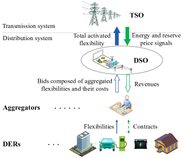
Figure 1: Framework of activating the flexibility of DERs to participate in the transmission system operation [4, 5, 6, 7].

In Fig. 1, the flexibility of individual DERs is first collected by their aggregators, who compensate DER users for activating their flexibility through contracts. Aggregators then calculate their aggregated flexibility and associated costs to bid in the distribution system’s flexibility market. The flexibility market is cleared by the DSO based on the price signals from the TSO and the bids from aggregators. The DSO then allocates the obtained revenue from the transmission level to aggregators. This framework, or similar ones, can be found in many existing studies [4, 5, 6, 7]. Ensuring that the DSO is non-profit in the flexibility market is essential for the framework to attract aggregators to participate and operate sustainably. In another flexibility activation framework, the DSO calculates security restrictions for each aggregator, and aggregators directly participate in the transmission system operation under these restrictions [8, 9]. This framework, however, leads to a potential conservativeness of each aggregator’s flexibility due to insufficient coordination among aggregators. Therefore, this paper focuses on the market framework shown in Fig. 1 that allows the DSO to coordinate aggregators to provide a larger total flexibility to the transmission system. Within this framework, the primary issue is how to formulate the aggregated flexibility and its associated price.

Numerous studies have focused on the modeling of aggregated flexibility, proposing models such as the power boundary model [10], power-energy boundary model [11, 12], vertex-based polytope [13], homothetic polytope [14], and $k$-order feasible region [15]. Yet, these studies do not discuss how to quantify the costs or values of the feasible regions determined by these aggregated flexibility models, which is essential to activate flexibility. Although the power boundary model offers a straightforward quantification method by defining prices for the adjustable power range in each time slot, just like conventional generators, it faces challenges in capturing the time-coupled characteristics of storage or storage-like DERs, e.g., BESSs, EVs, and HPs. Within the research focusing on DSO flexibility markets, defining and formulating flexibility prices is always a fundamental part. Existing research in this field predominantly formulates flexibility prices based on the power adjustment range relative to the reference or baseline power in each time slot [4, 16, 5, 17, 18, 19].

The advantages of flexibility pricing based on power adjustment ranges are its intuitive calculation and uniformity with generators. However, as mentioned before, this pricing scheme is insufficient to quantify the time-coupled flexibility offered by storage-like DERs. Besides, the potential inconvenience caused to DER users by flexibility activation, which is the fundamental reason for flexibility costs, cannot be adequately quantified by the power range alone (detailed discussions on this fact will be provided in Section II). In [9], the opportunity cost is used to evaluate the cost of EVs’ mid-term flexibility, but this method cannot be directly generalized to various heterogeneous DERs, limiting its application in a unified DSO flexibility market with multiple types of DERs.

In summary, there is a lack of discussion on the pricing method of the time-coupled flexibility and the associated flexibility market. Filling this gap enables a more reasonable evaluation of the costs and values of DERs’ flexibility, fostering a more effective DSO flexibility market and enhancing the willingness of DER users to offer their flexibility to contribute to power systems operation. Therefore, this paper proposes a direct flexibility pricing method aligned with the time-coupled flexibility models. Moreover, we design a DSO flexibility market model to activate the flexibility of DERs to participate in the transmission system operation for energy arbitrage and ancillary services provision. The contributions are threefold:

• From the perspective of DER users, we propose to compute the flexibility cost based on activated adjustment ranges in both power and accumulated energy consumption. This method is in line with the power-energy boundary models of individual DERs’ flexibility and is able to quantify the potential inconvenience caused to users by flexibility activation, which is more suitable for typical DERs such as EVs, BESSs, and HPs compared to the traditional power range-based approach.

• From the aggregators’ standpoint, we propose to compute their flexibility costs directly according to the activated area of the aggregated flexibility model. Unlike the traditional power range-based formulations, the proposed approach aligns with the aggregated flexibility model with time coupling, thus allowing aggregators to define their cost coefficients directly based on the feasible regions determined by their flexibility models.

• From the DSO’s perspective, we propose a market-clearing model for activating the flexibility of all aggregators in the distribution system to participate in the transmission system operation for energy arbitrage and reserve services provision. Based on this model, we propose the concept of marginal flexibility price for distributing revenues earned from the transmission level to each aggregator, ensuring incentive compatibility, revenue adequacy, and a non-profit DSO.

Notations: Bold letters (e.g., $\mathbf{x}$, $\mathbf{A}$) denote vectors and matrices, and the corresponding regular letters with subscripts represent their components. The operator $(\cdot)^{\top}$ calculates the vector/matrix transposition, and the operator $|(\cdot)|$ calculates the cardinality of a set.

II Flexibility Cost Formulation of DERs based on Both Power and Energy Adjustment Ranges

This section first presents the proposed unified flexibility cost formulation based on the adjustment ranges in both power and accumulated energy consumption. We then discuss how to specify the cost coefficients in this formulation according to the distinct operational characteristics of typical DERs.

II-A Unified Formulation for Flexibility Costs

Flexibility refers to the capability of a device to adjust its operation. From the power system’s perspective, the flexibility cost of a device should be computed by the adjustment range it provides, similar to the capacity costs for generators providing ancillary services. The proposed flexibility cost formulation is based on adjustment ranges in both power and accumulated energy, which aligns with the classic power-energy flexibility model of individual DERs [11]. Besides, this proposed flexibility cost formulation can quantify the potential inconvenience caused to DER users upon flexibility activation.

We discretize the time horizon into $T$ slots, each of a length $\Delta_{T}$, indexed by $t$, and denote the whole time horizon as $[T]\triangleq\{1,2,...,T\}$. The flexibility cost of one DER is:

$$C_{\text{DER}}={\hat{\mathbf{c}}_{\text{p}}^{\top}\Delta\hat{\mathbf{p}}+\check{\mathbf{c}}_{\text{p}}^{\top}\Delta\check{\mathbf{p}}+\hat{\mathbf{c}}_{\text{e}}^{\top}\Delta\hat{\mathbf{e}}+\check{\mathbf{c}}_{\text{e}}^{\top}\Delta\check{\mathbf{e}}},$$ (1)

where $\Delta\hat{\mathbf{p}}\in\mathbb{R}^{T}_{+}$ and $\Delta\check{\mathbf{p}}\in\mathbb{R}^{T}_{+}$ denote the vectors of activated upward and downward adjustment ranges of the power profile $\mathbf{p}\in\mathbb{R}^{T}$ relative to the baseline profile $\mathbf{p}^{{\text{base}}}\in\mathbb{R}^{T}$, respectively; $\Delta\hat{\mathbf{e}}\in\mathbb{R}^{T}_{+}$ and $\Delta\check{\mathbf{e}}\in\mathbb{R}^{T}_{+}$ represent the activated upward and downward adjustment ranges of the accumulated energy consumption trajectory $\mathbf{e}\in\mathbb{R}^{T}$ relative to the baseline energy trajectory $\mathbf{e}^{{\text{base}}}\in\mathbb{R}^{T}$, respectively; $\hat{\mathbf{c}}_{\text{p}}\in\mathbb{R}^{T}$, $\check{\mathbf{c}}_{\text{p}}\in\mathbb{R}^{T}$, $\hat{\mathbf{c}}_{\text{e}}\in\mathbb{R}^{T}$, and $\check{\mathbf{c}}_{\text{e}}\in\mathbb{R}^{T}$ denote the vectors of cost coefficients for upward and downward adjustment ranges in power and energy, depending on the specific DERs. Variables $\mathbf{p}$, $\Delta\hat{\mathbf{p}}$, $\Delta\check{\mathbf{p}}$, $\mathbf{e}$, $\Delta\hat{\mathbf{e}}$, and $\Delta\check{\mathbf{e}}$ should fulfill the following constraints:

$$\underline{\mathbf{p}}\leq\mathbf{p}^{{\text{base}}}-\Delta\check{\mathbf{p}}\leq\mathbf{p}\leq\mathbf{p}^{{\text{base}}}+\Delta\hat{\mathbf{p}}\leq\overline{\mathbf{p}},$$ (2)

$$\underline{\mathbf{e}}\leq\mathbf{e}^{{\text{base}}}-\Delta\check{\mathbf{e}}\leq\mathbf{e}\leq\mathbf{e}^{{\text{base}}}+\Delta\hat{\mathbf{e}}\leq\overline{\mathbf{e}},$$ (3)

$$e_{t}^{{\text{base}}}=\sum\limits_{\tau=1}^{t}{p_{\tau}^{{\text{base}}}\Delta_{T}},e_{t}=\sum\limits_{\tau=1}^{t}{p_{\tau}\Delta_{T}},\forall t\in[T],$$ (4)

where $\overline{\mathbf{p}}\in\mathbb{R}^{T}$, $\underline{\mathbf{p}}\in\mathbb{R}^{T}$, $\overline{\mathbf{e}}\in\mathbb{R}^{T}$, and $\underline{\mathbf{e}}\in\mathbb{R}^{T}$ denotes the DER’s physical upper and lower bounds of power and accumulated energy. Constraints (2) and (3) restrict the power and energy adjustment ranges within their physical bounds. Equation (4) gives the relationship between power and energy.

The constraints in (2)-(4) actually constitute the power-energy boundary model that describes the flexibility of typical DERs, with bound parameters determined by the operational characteristics of different DERs, as detailed in [11]. The formulation (1) aligns with the flexibility model (2)-(4) since it calculates the flexibility cost based on the activated adjustment ranges in both power and accumulated energy consumption. By properly setting the cost coefficient vectors $\hat{\mathbf{c}}_{\text{p}}$, $\check{\mathbf{c}}_{\text{p}}$, $\hat{\mathbf{c}}_{\text{e}}$, and $\check{\mathbf{c}}_{\text{e}}$, the flexibility cost (1) can reflect the potential inconvenience caused to DER users upon flexibility activation, which will be discussed in the next subsection.

II-B Specification of the Cost Coefficients for Typical DERs

For resources whose costs are directly quantified by power adjustment ranges, like distributed PV and curtailable loads, specifying the cost coefficients is straightforward: set $\hat{\mathbf{c}}_{\text{e}}$ and $\check{\mathbf{c}}_{\text{e}}$ to zero and specify $\hat{\mathbf{c}}_{\text{p}}$ and $\check{\mathbf{c}}_{\text{p}}$ identically as the traditional power range-based formulations. Hence, the rest of this subsection mainly discusses how to specify the cost coefficients for typical storage-like DERs, including EVs, BESS, and HPs, based on the potential inconvenience caused to users of these DERs upon flexibility activation.

II-B1 Electric Vehicles

The flexibility of EVs lies in the charging process during their plug-in periods. Since the primary goal of EV charging is to charge the battery to the expected energy level by departure, the inconvenience caused to EV users by activating this flexibility is reflected in the potentially unsatisfied charging demand at the departure time.

Fig. 2 illustrates a typical EV’s adjustment ranges in the accumulated energy consumption and its flexibility cost coefficients. In this example, the EV has an expected value for the energy to be charged by departure but also allows it to be adjustable within certain upper and lower bounds. The upper bound typically corresponds to the battery’s capacity limit, while the lower bound represents the minimum energy level acceptable to the EV user. The baseline energy trajectory is the energy trajectory where charging starts immediately at the rated power upon plug-in until the expected energy level is reached. The area within the upward and downward energy adjustment ranges represents the activated flexibility in accumulated energy consumption, which is where the actual energy trajectory can be adjusted. However, only the energy adjustment at the departure time can cause inconvenience to the EV user. More precisely, it is the downward adjustment that matters, as the upward adjustment, representing charging more than the expected energy, typically does not lead to an inconvenience in the EV’s usage. Thus, in the flexibility cost coefficients, only the coefficient for the downward energy adjustment range $\check{\mathbf{c}}_{\text{e}}$ at the departure time is non-zero, while $\check{\mathbf{c}}_{\text{e}}$ at other times, $\hat{\mathbf{c}}_{\text{e}}$, $\check{\mathbf{c}}_{\text{p}}$ and $\hat{\mathbf{c}}_{\text{p}}$ are all zero.

Figure 2: The flexibility in accumulated energy consumption of an EV and its associated cost coefficients.

In summary, based on the flexibility cost model (1), the aggregator can establish a contract with EV users that specifies compensation for any unsatisfied charging demands at the departure time. This contract directly correlates to the value of $\check{\mathbf{c}}_{\text{e}}$. Consequently, EV users can intuitively understand the potential inconvenience to their EV usage due to flexibility activation and evaluate their expected benefits. This level of clarity and directness is not achievable with traditional cost quantification methods based on power adjustment ranges, as power adjustments during charging are invisible to EV users.

II-B2 Battery Energy Storage Systems

The flexibility of a BESS lies in its ability to charge and discharge within the battery’s capacity. The energy level of a BESS typically needs periodic balancing to preserve sufficient capacity for potential charging and discharging demands. Therefore, the inconvenience caused to a BESS user by flexibility activation can be quantified by the unbalanced energy at times of balancing.

Fig. 3 illustrates a typical BESS’s energy adjustment range and the corresponding cost coefficients. Three balancing points are set in the decision time horizon, at which the BESS user receives compensation if its energy does not return to the initial level. This compensation is translated into the settings of cost coefficients, where both $\hat{\mathbf{c}}_{\text{e}}$ and $\check{\mathbf{c}}_{\text{e}}$ are nonzero at the pre-defined balancing times. The cost coefficient for the downward energy adjustment range $\check{\mathbf{c}}_{\text{e}}$ is set larger than that for upward capacity $\hat{\mathbf{c}}_{\text{e}}$, indicating that compensation for insufficient energy is larger than that for overcharged energy. Cost coefficients at the end of the time horizon $T$ are higher than those at other balancing times, indicating the highest priority of the energy balancing across the whole time horizon. This balance may also be imposed as a hard constraint by setting the upper and lower energy bounds at the end of the time horizon to zero, ensuring the battery’s energy finally returns to the initial level.

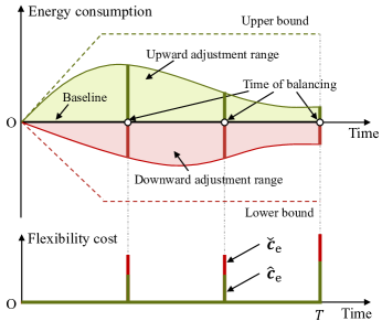
Figure 3: The flexibility in accumulated energy consumption of a BESS and its associated cost coefficients.

II-B3 Heat Pumps

HPs can offer flexibility to the power system due to the allowable adjustment range in the buildings’ indoor temperature. Hence, temperature adjustment ranges associated with the activated flexibility most appropriately measure the potential inconvenience caused to HP users. The indoor temperature evolution of a building with an HP can be approximately described using the linear thermal dynamic model [20]:

$${\theta_{t}}=\alpha{\theta_{t-1}}+(1-\alpha)(\theta_{t}^{{\text{amb}}}+\frac{{\eta}}{H}\cdot{p_{t}}),\forall t\in[T],$$ (5)

where ${\theta_{t}}$ denotes the indoor temperature in Kelvin (K) in the $t$-th time slot, $\alpha=\exp(-{\Delta_{T}H}/{C})$, $C$ and $H$ are the thermal capacitance (kWh/K) and resistance (K/kW), $\theta_{t}^{{\text{amb}}}$ represents the ambient temperature, and $\eta$ is the coefficient of performance (COP) of the HP (assumed constant).

We define the baseline power and accumulated energy consumption profiles to always maintain the indoor temperature at the set point $\theta^{\text{set}}_{t},\forall t\in[T]$. Activating the flexibility of HPs leads to the fluctuation of indoor temperature within the upward and downward adjustment ranges relative to the temperature set point, denoted by $\Delta\hat{\theta}_{t}$ and $\Delta\check{\theta}_{t}$, respectively, (with vector forms $\Delta\hat{\boldsymbol{\theta}}\in\mathbb{R}^{T}_{+}$ and $\Delta\check{\boldsymbol{\theta}}\in\mathbb{R}^{T}_{+}$). Regarding the relationship between the temperature adjustment ranges, $\Delta\hat{\boldsymbol{\theta}}$ and $\Delta\check{\boldsymbol{\theta}}$, and the upward and downward adjustment ranges in power, $\Delta\hat{\mathbf{p}}$ and $\Delta\check{\mathbf{p}}$, and accumulated energy consumption, $\Delta\hat{\mathbf{e}}$ and $\Delta\check{\mathbf{e}}$, the following Proposition holds:

Proposition 1

The upward and downward temperature adjustment ranges, $\Delta\hat{\boldsymbol{\theta}}$ and $\Delta\check{\boldsymbol{\theta}}$, can be linearly transformed into the upward and downward adjustment ranges in accumulated energy consumption, $\Delta\hat{\mathbf{e}}$ and $\Delta\check{\mathbf{e}}$, respectively, by:

$$\Delta\hat{\mathbf{e}}={\mathbf{D}}\Delta\hat{\boldsymbol{\theta}},\;\;\Delta\check{\mathbf{e}}={\mathbf{D}}\Delta\check{\boldsymbol{\theta}},$$ (6)

where ${\mathbf{D}}$ is a $T\times T$ invertible matrix, defined as:

$${\mathbf{D}}\triangleq\Delta_{T}\cdot\frac{H}{\eta}\left[{\begin{array}[]{cccc}1&{}\hfil&{}\hfil&{}\hfil\\ {1-\alpha}&1&{}\hfil&{}\hfil\\ \vdots&\ddots&\ddots&{}\hfil\\ {1-\alpha}&\cdots&{1-\alpha}&1\end{array}}\right].$$

However, $\Delta\hat{\boldsymbol{\theta}}$ and $\Delta\check{\boldsymbol{\theta}}$ cannot be respectively transformed into upward and downward power adjustment ranges $\Delta\hat{\mathbf{p}}$ and $\Delta\check{\mathbf{p}}$.

Proof: See Appendix A.

The rationale behind Proposition 1 can be intuitively understood as follows: the indoor temperature is primarily influenced by the accumulated power over time rather than the power in each time slot itself. The transformation in (6) allows aggregators to have a contract with HP users specifying the compensation for per unit temperature adjustment range and to transform this compensation into cost coefficients of energy adjustment range. We denote by $\hat{\boldsymbol{\rho}}\in\mathbb{R}^{T}_{+}$ and $\check{\boldsymbol{\rho}}\in\mathbb{R}^{T}_{+}$ the vectors of compensations for the activated upward and downward temperature adjustment ranges, respectively. Then, the total cost of the activated flexibility of an HP is:

$$C_{\text{HP}}=\hat{\boldsymbol{\rho}}^{\top}\Delta\hat{\boldsymbol{\theta}}+\check{\boldsymbol{\rho}}^{\top}\Delta\check{\boldsymbol{\theta}},$$

which can then be equivalently reformulated based on energy adjustment ranges:

$$C_{\text{HP}}=\hat{\boldsymbol{\rho}}^{\top}\mathbf{D}^{-1}\Delta\hat{\mathbf{e}}+\check{\boldsymbol{\rho}}^{\top}\mathbf{D}^{-1}\Delta\check{\mathbf{e}},$$

aligning with the flexibility cost model (1), where $\hat{\mathbf{c}}_{\text{p}}=\check{\mathbf{c}}_{\text{p}}=\mathbf{0}$, $\hat{\mathbf{c}}_{\text{e}}=(\mathbf{D}^{-1})^{\top}\hat{\boldsymbol{\rho}}$, and $\check{\mathbf{c}}_{\text{e}}=(\mathbf{D}^{-1})^{\top}\check{\boldsymbol{\rho}}$.

Fig. 4 illustrates adjustment ranges in the indoor temperature, the corresponding adjustment ranges in accumulated energy consumption, and cost coefficients. Cost coefficients of energy adjustment ranges shown in this figure, which increase with time, are generated based on a constant cost coefficient of temperature adjustment range across the time horizon. Take $\check{\mathbf{c}}_{\text{e}}$ as an example, assuming that $\check{\rho}_{t}=\check{\rho}_{0},\forall t\in[T]$, then $\check{\mathbf{c}}_{\text{e}}=([\check{\rho}_{0},\check{\rho}_{0},\cdots,\check{\rho}_{0}]\mathbf{D}^{-1})^{\top}=\frac{\eta}{H\Delta_{T}}\check{\rho}_{0}[{\alpha^{T-1}},...,{\alpha^{2}},\alpha,1]^{\top}$. As $0<\alpha<1$ by definition, $\check{c}_{\text{e},t}$ increases with the time index $t$. Besides, $\check{\mathbf{c}}_{\text{e}}$ is typically larger than $\hat{\mathbf{c}}_{\text{e}}$ because downward temperature adjustments cause more discomfort to the people inside the building than upward adjustments considering the primary task of the HP is heating.

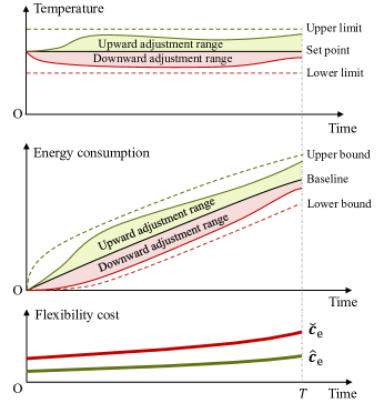
Figure 4: The flexibility in accumulated energy consumption of an HP and its associated cost coefficients.

Finally, we note that $\hat{\boldsymbol{\rho}}$ and $\check{\boldsymbol{\rho}}$ should not be uniform across all buildings, as the thermal dynamic parameters and HPs’ COPs vary. Identical temperature adjustments can lead to different energy adjustments in different buildings, so applying uniform $\hat{\boldsymbol{\rho}}$ and $\check{\boldsymbol{\rho}}$ would be unfair to HP users in a well-insulated building. Thus, $\hat{\boldsymbol{\rho}}$ and $\check{\boldsymbol{\rho}}$ should be customized based on the thermal dynamic parameters of the building and the HP’s COP. We suggest setting $\hat{\boldsymbol{\rho}}$ and $\check{\boldsymbol{\rho}}$ proportional to $\frac{H\Delta_{T}}{\eta}$, which aligns the HP’s flexibility cost coefficients with the contribution to energy adjustment ranges.

III Model and Cost for Aggregated Flexibility

We have discussed the flexibility cost formulation for individual DERs. This section focuses on the aggregator’s perspective, namely the model and cost for the aggregated flexibility, which provides the bidding information of aggregators in the DSO flexibility market. We denote the set of DERs in the aggregator as $\mathcal{K}$, indexed by $k$, and the power vector of the $k$-th DER as $\mathbf{p}_{k}\in\mathbb{R}^{T}$. Hence, the aggregated power is $\mathbf{P}\triangleq\sum\nolimits_{k\in\mathcal{K}}\mathbf{p}_{k}$. The aggregated flexibility model refers to the feasible region of $\mathbf{P}$. Given the individual flexibility constraints (2)-(4), the aggregated flexibility, as derived in our previous works [15] and [21], can be formulated as follows:

$$\underline{\boldsymbol{\phi}}\leq{\mathbf{UP}}\leq\overline{\boldsymbol{\phi}},$$ (7)

where $\mathbf{U}$ is an ${M\times T}$ coefficient matrix with each row vector being a ${1\times T}$ vector composed of 0s and 1s, and $M$ represents the number of constraints that is dependent on whether an exact or an approximate model is used. Constraints (7) define a polytope in the $\mathbb{R}^{T}$ space with a specific shape. We let $\mathbb{B}\triangleq\{0,1\}$ and $\mathbb{B}^{T}$ denote the the set of all $T$-dimensional row vectors composed solely of 0s and 1s. If the row vectors of $\mathbf{U}$ span $\mathbb{B}^{T}$ except for $\mathbf{0}$, i.e., $M=2^{T}-1$, $\mathbf{U}$ corresponds to the exact aggregation model. When the row vector set of $\mathbf{U}$ is a subset of $\mathbb{B}^{T}$, $\mathbf{U}$ corresponds to an approximate model. Bound parameters $\underline{\boldsymbol{\phi}}\in\mathbb{R}^{M}$ and $\overline{\boldsymbol{\phi}}\in\mathbb{R}^{M}$ are derived from all the individual power and energy bound parameters in (2)-(3). Reducing the number of rows of $\mathbf{U}$ creates an approximate model with low complexity, and appropriately adjusting $\underline{\boldsymbol{\phi}}$ and $\overline{\boldsymbol{\phi}}$ forms either an outer or inner approximation. For example, setting the coefficient matrix $\mathbf{U}$ to only include power and accumulated energy constraints and the bound parameters $\underline{\boldsymbol{\phi}}$ and $\overline{\boldsymbol{\phi}}$ to the sum of all individual power and energy bounds yields an outer approximation [15], and properly shrinking the gap between $\underline{\boldsymbol{\phi}}$ and $\overline{\boldsymbol{\phi}}$ forms an inner approximation [21].

We are now ready to introduce the flexibility cost formulation for the aggregated flexibility model (7). For the sake of clarity, we hereafter refer to the product of $\mathbf{U}$ and the aggregated power profile $\mathbf{P}$, i.e., $\mathbf{UP}$, as the flexibility trajectory and the product of $\mathbf{U}$ and the aggregated baseline power profile $\mathbf{UP}^{\text{base}}$, i.e., $\mathbf{UP}^{\text{base}}$, as the baseline flexibility trajectory. Similar to the flexibility model (2)-(4) for individual DERs, activating the aggregated flexibility means that the flexibility trajectory $\mathbf{UP}$ can deviate within a certain range relative to the baseline trajectory $\mathbf{UP}^{\text{base}}$, which can be formulated as:

$$\underline{\boldsymbol{\phi}}\leq\mathbf{UP}^{\text{base}}-\Delta\check{\boldsymbol{\phi}}\leq\mathbf{UP}\leq\mathbf{UP}^{{\text{base}}}+\Delta\hat{\boldsymbol{\phi}}\leq\overline{\boldsymbol{\phi}},$$ (8)

where $\Delta\hat{\boldsymbol{\phi}}\in\mathbb{R}^{M}_{+}$ and $\Delta\check{\boldsymbol{\phi}}\in\mathbb{R}^{M}_{+}$ are the activated upward and downward adjustment ranges, respectively. The utility function of the aggregator is defined as a linear function with the activated upward and downward adjustment ranges, that is

$$C_{\text{agg}}=\hat{\mathbf{c}}_{\text{agg}}^{\top}\Delta\hat{\boldsymbol{\phi}}+\check{\mathbf{c}}_{\text{agg}}^{\top}\Delta\check{\boldsymbol{\phi}},$$ (9)

where $\hat{\mathbf{c}}_{\text{agg}}$ and $\check{\mathbf{c}}_{\text{agg}}$ in $\mathbb{R}^{M}_{+}$ denote the upward and downward cost coefficients for flexibility adjustment ranges, respectively, which the aggregator bids to the DSO market.

The next question is how the aggregator can calculate the cost coefficients $\hat{\mathbf{c}}_{\text{agg}}$ and $\check{\mathbf{c}}_{\text{agg}}$. Principally, $\hat{\mathbf{c}}_{\text{agg}}$ and $\check{\mathbf{c}}_{\text{agg}}$ are related to the aggregator’s cost of purchasing flexibility from the DER users and its operation costs. Aggregators may develop various strategies to determine $\hat{\mathbf{c}}_{\text{agg}}$ and $\check{\mathbf{c}}_{\text{agg}}$ for bidding in the DSO flexibility market. Since the focus of this paper is primarily on the formulation of flexibility costs, we here use a simple approach to estimate $\hat{\mathbf{c}}_{\text{agg}}$ and $\check{\mathbf{c}}_{\text{agg}}$ without a detailed discussion of the bidding strategies of aggregators.

First, it should be noted that the flexibility model (7) includes constraints of power and accumulated energy consumption of the aggregator. In other words, the power and accumulated energy consumption are a part of the flexibility trajectory $\mathbf{UP}$. The power and accumulated energy part of cost coefficients $\hat{\mathbf{c}}_{\text{agg}}$ and $\check{\mathbf{c}}_{\text{agg}}$ are estimated via a weighted average method, with the weights being the ratio of the maximum power and energy adjustment ranges of each DER, i.e.,

$$\hat{c}_{\text{agg},m}=\frac{{\sum\nolimits_{k\in{{\mathcal{K}}}}{\hat{c}_{k,m}\left({{{\overline{\phi}}_{k,m}}-\phi_{k,m}^{{\text{base}}}}\right)}}}{{\sum\nolimits_{k\in{{\mathcal{K}}}}{\left({{{\overline{\phi}}_{k,m}}-\phi_{k,m}^{{\text{base}}}}\right)}}},\forall m\in\mathcal{I}_{\text{p,e}},$$ (10)

$$\check{c}_{\text{agg},m}=\frac{{\sum\nolimits_{k\in{{\mathcal{K}}}}{\check{c}_{k,m}\left({\phi_{k,m}^{{\text{base}}}-{{\underline{\phi}}_{k,m}}}\right)}}}{{\sum\nolimits_{k\in{{\mathcal{K}}}}{\left({\phi_{k,m}^{{\text{base}}}-{{\underline{\phi}}_{k,m}}}\right)}}},\forall m\in\mathcal{I}_{\text{p,e}}$$ (11)

where $k$ is the index of DERs and $\mathcal{K}$ is the set of all DERs within the aggregator; $m$ is the index of constraints in the aggregated flexibility model, and $\mathcal{I}_{\text{p,e}}$ is the indices set of constraints on power and accumulated energy consumption, $|\mathcal{I}_{\text{p,e}}|\leq M$. The parameter $\phi_{k,m}^{{\text{base}}}$ denotes the baseline of power or accumulated energy consumption of the $k$-th DER, depending on whether $m$ corresponds to a constraint on power or accumulated energy consumption. Similarly, $\overline{\phi}_{k,m}$ and $\underline{\phi}_{k,m}$ respectively denote the upper and lower bounds of power or accumulated energy consumption, and $\hat{c}_{k,m}$ and $\check{c}_{k,m}$ are the cost coefficients of the adjustment ranges in power or accumulated energy consumption specified in Section II.

If the aggregated flexibility model (7) includes constraints beyond power and accumulated energy consumption, i.e., $M>|\mathcal{I}_{\text{p,e}}|$, the cost coefficients of adjustment ranges in those additional parts should be directly set to zero. This setting avoids the duplication of the cost calculation, as power and accumulated energy adjustments could lead to adjustments in other segments of the flexibility trajectory. This does not imply that other segments of the flexibility trajectory do not contribute to the flexibility cost of the aggregator since those segments are subject to constraints and indirectly influence the aggregator’s total flexibility cost $C_{\text{agg}}$. Indeed, for simplicity, the DSO can require aggregators to model their flexibility using only power and accumulated energy constraints and to submit the cost coefficients only for adjustment ranges in this segment. Nevertheless, since we have designed a more general flexibility cost formulation, it holds the potential to be applied to DSO markets with more accurate flexibility models.

IV DSO Flexibility Market Clearing and Marginal Flexibility Prices

We consider the scenario where the DSO procures flexibility from aggregators for energy arbitrage and reserve service provision at the transmission level. The DSO flexibility market should 1) determine the reference power profile and reserve capacities offered to the transmission system, 2) determine the activated adjustment range for the flexibility trajectory of each aggregator within the distribution system, and 3) distribute the revenues obtained from the transmission level to each aggregator while ensuring incentive compatibility, revenue adequacy, and a non-profit DSO.

IV-A Modeling of the DSO Flexibility Market Clearing

The objective of the DSO flexibility market clearing is to maximize social welfare, which is equivalent to minimizing the net cost of the distribution system in this paper, formulated as:

$$\min C_{\text{net}} ={C_{{\text{Energy}}}}-{R_{{\text{Capacity}}}}+{C_{{\text{Flexibility}}}},$$ (12)

$${C_{{\text{Energy}}}} \triangleq{{\mathbf{c}}_{\text{energy}}^{\top}}{{\mathbf{P}}^{\text{ref}}_{0}},$$

$${R_{\text{Capacity}}} \triangleq{\mathbf{c}}_{\text{ru}}^{\top}{{\mathbf{R}}^{\text{up}}}+{\mathbf{c}}_{\text{rd}}^{\top}{{\mathbf{R}}^{\text{dn}}},$$

$${C_{{\text{Flexibility}}}} \triangleq\sum\nolimits_{h\in\mathcal{A}}{(\hat{\mathbf{c}}_{h}^{\top}\Delta\hat{\boldsymbol{\phi}}_{h}+\check{\mathbf{c}}_{h}^{\top}\Delta\check{\boldsymbol{\phi}}_{h})},$$

where ${C_{{\text{Energy}}}}$ is the total energy cost of the distribution system, ${R_{\text{Capacity}}}$ is the revenue from providing reserve capacities, and ${C_{{\text{Flexibility}}}}$ is the total flexbility cost; ${\mathbf{c}}_{\text{energy}}\in\mathbb{R}^{T}$, ${\mathbf{c}}_{\text{ru}}\in\mathbb{R}^{T}$, and ${\mathbf{c}}_{\text{rd}}\in\mathbb{R}^{T}$ denote the vectors composed of the energy price, up-reserve price and down-reserve price, respectively, at the transmission level over the time horizon $[T]$ (assuming that the DSO acts as a price taker at the transmission system, ${\mathbf{c}}_{\text{energy}}$ , ${\mathbf{c}}_{\text{ru}}$, and ${\mathbf{c}}_{\text{rd}}$ are input parameters in the DSO flexibility market); ${{\mathbf{P}}^{\text{ref}}_{0}}\in\mathbb{R}^{T}$ represents the reference power profile at the transmission-distribution interface, i.e., the root node of the distribution system, while ${{\mathbf{R}}^{\text{up}}}\in\mathbb{R}^{T}_{+}$ and ${{\mathbf{R}}^{\text{dn}}}\in\mathbb{R}^{T}_{+}$ represent the up- and down-reserve capacities offered to the transmission system, respectively; aggregators in the distribution system are indexed by $h$, with the set of all aggregators denoted as $\mathcal{A}$; $\Delta\hat{\boldsymbol{\phi}}_{h}$ and $\Delta\check{\boldsymbol{\phi}}_{h}$ denote the activated upward and downward adjustment range of the flexibility trajectory of aggregator $h$, respectively, and $\hat{\mathbf{c}}_{h}$ and $\check{\mathbf{c}}_{h}$ denote the corresponding flexibility cost coefficients, as defined in Section III.

The DSO’s reserve capacity offered to the transmission system must ensure that any adjustment signal within this capacity is feasible with respect to both the distribution network constraints and aggregators’ flexibility constraints, which means the following condition should be satisfied:

$${{\mathbf{P}}_{0}}\in\mathbb{X},\forall{{\mathbf{P}}_{0}}:{\mathbf{P}}_{0}^{{\text{ref}}}-{{\mathbf{R}}^{{\text{up}}}}\leq{{\mathbf{P}}_{0}}\leq{\mathbf{P}}_{0}^{{\text{ref}}}+{{\mathbf{R}}^{{\text{dn}}}},$$ (13)

where $\mathbb{X}$ represents the feasible region of the power profile ${{\mathbf{P}}_{0}}\in\mathbb{R}^{T}$ at the root node of the distribution system, determined by the distribution power flow constraints and the flexibility models of all aggregators. The upper and lower bounds of ${{\mathbf{P}}_{0}}$ are ${\mathbf{P}}_{0}^{{\text{ref}}}+{{\mathbf{R}}^{{\text{dn}}}}$ and ${\mathbf{P}}_{0}^{{\text{ref}}}-{{\mathbf{R}}^{{\text{up}}}}$, respectively. Down-reserve is related to the plus sign, and up-reserve is related to the minus sign because reserves are defined from the perspective of generators, whereas ${\mathbf{P}}_{0}^{{\text{ref}}}$ and ${{\mathbf{P}}_{0}}$ represent loads with an opposite direction. As we employ the LinDistFlow model to describe the distribution power flow constraints, and the aggregated flexibility model (7) is also linear, the feasible region $\mathbb{X}$ is a convex polytope. Consequently, the condition (13) becomes equivalent to ${\mathbf{P}}_{0}^{{\text{ref}}}-{{\mathbf{R}}^{{\text{up}}}}\in\mathbb{X}$ and ${\mathbf{P}}_{0}^{{\text{ref}}}+{{\mathbf{R}}^{{\text{dn}}}}\in\mathbb{X}$. For the sake of brevity, we let

$${{\mathbf{P}}^{{\text{ru}}}_{0}}\triangleq{{\mathbf{P}}^{{\text{ref}}}_{0}}-{{\mathbf{R}}^{{\text{up}}}}\;\;\;\;\text{and}\;\;\;\;{{\mathbf{P}}^{{\text{rd}}}_{0}}\triangleq{{\mathbf{P}}^{{\text{ref}}}_{0}}+{{\mathbf{R}}^{{\text{dn}}}}$$ (14)

denote the power profiles at the root node of the distribution system corresponding to the upper and lower bounds of the reserve capacity, respectively, and let $\mathcal{W}\triangleq\{\text{ru,rd}\}$ denote the set of superscripts representing up- and down-reserves.

Constraints in the DSO flexibility market include:

$${\mathbf{P}}_{0}^{\omega}=\sum\nolimits_{j\in 0}{{\mathbf{P}}_{0j}^{\omega}},\forall\omega\in{{\mathcal{W}}},$$ (15)

$$\sum\nolimits_{j\in i}{{\mathbf{P}}_{ij}^{\omega}}+{\mathbf{P}}_{i}^{{\text{fix}}}+{\mathbf{P}}_{i}^{{\text{flex,}}\omega}={\mathbf{0}},\forall i\in{\mathcal{N}}_{+},\omega\in{{\mathcal{W}}},$$ (16)

$$\sum\nolimits_{j\in i}{{\mathbf{Q}}_{ij}^{\omega}}+{\mathbf{Q}}_{i}^{{\text{fix}}}+{\mathbf{Q}}_{i}^{{\text{flex,}}\omega}={\mathbf{0}},\forall i\in{\mathcal{N}}_{+},\omega\in{{\mathcal{W}}},$$ (17)

$${\mathbf{V}}_{i}^{\omega}-{{\mathbf{V}}_{j}^{\omega}}=2({r_{ij}}{{\mathbf{P}}_{ij}^{\omega}}+{x_{ij}}{{\mathbf{Q}}_{ij}^{\omega}}),\forall ij\in{{\mathcal{L}}},\omega\in{{\mathcal{W}}},$$ (18)

$${\mathbf{V}}_{0}^{\omega}={\mathbf{1}},\forall\omega\in{{\mathcal{W}}},$$ (19)

$${\underline{\mathbf{V}}_{i}}\leq{\mathbf{V}}_{i}^{\omega}\leq{\overline{\mathbf{V}}_{i}},\forall i\in{\mathcal{N}}_{+},\omega\in{{\mathcal{W}}},$$ (20)

$${\mathbf{P}}_{i}^{{\text{flex,}}\omega}=\sum\nolimits_{h\in{{{\mathcal{A}}}_{i}}}{{\mathbf{P}}_{h}^{\omega}},\forall i\in{\mathcal{N}}_{+},\omega\in{{\mathcal{W}}},$$ (21)

$${\mathbf{Q}}_{i}^{{\text{flex,}}\omega}=\sum\nolimits_{h\in{{{\mathcal{A}}}_{i}}}{{\mathbf{Q}}_{h}^{\omega}},\forall i\in{\mathcal{N}}_{+},\omega\in{{\mathcal{W}}},$$ (22)

$${\mathbf{Q}}_{h}^{\omega}={\mathbf{P}}_{h}^{\omega}\tan{\gamma_{h}},\forall h\in{{\mathcal{A}}},\omega\in{{\mathcal{W}}},$$ (23)

$${{\mathbf{U}}_{h}}{\mathbf{P}}_{h}^{\omega}\leq{{\mathbf{U}}_{h}}{\mathbf{P}}_{h}^{{\text{base}}}+\Delta\hat{\boldsymbol{\phi}}_{h}:\hat{\boldsymbol{\lambda}}_{h}^{\omega},\forall h\in{{\mathcal{A}}},\omega\in{{\mathcal{W}}},$$ (24)

$${{\mathbf{U}}_{h}}{\mathbf{P}}_{h}^{\omega}\geq{{\mathbf{U}}_{h}}{\mathbf{P}}_{h}^{{\text{base}}}-\Delta\check{\boldsymbol{\phi}}_{h}:\check{\boldsymbol{\lambda}}_{h}^{\omega},\forall h\in{{\mathcal{A}}},\omega\in{{\mathcal{W}}},$$ (25)

$${{\mathbf{U}}_{h}}{\mathbf{P}}_{h}^{{\text{base}}}+\Delta\hat{\boldsymbol{\phi}}_{h}\leq{\overline{\boldsymbol{\phi}}_{h}},\forall h\in{{\mathcal{A}}},$$ (26)

$${{\mathbf{U}}_{h}}{\mathbf{P}}_{h}^{{\text{base}}}-\Delta\check{\boldsymbol{\phi}}_{h}\geq{\underline{\boldsymbol{\phi}}_{h}},\forall h\in{{\mathcal{A}}},$$ (27)

$$\Delta\hat{\boldsymbol{\phi}}_{h}\geq\mathbf{0},\Delta\check{\boldsymbol{\phi}}_{h}\geq\mathbf{0},\forall h\in{{\mathcal{A}}},$$ (28)

where $i/\mathcal{N}$ denotes the index/set of nodes in the distribution system, $0$ represents the root node, and $\mathcal{N}_{+}\triangleq\mathcal{N}\backslash\{0\}$; $\mathcal{L}$ denotes the set of lines where $ij$ refers to the line between node $i$ and node $j$; $j\in i$ indicates that node $j$ is connected to node $i$; $\mathcal{A}_{i}$ denotes the set of aggregators located at node $i$, $\bigcup_{i\in\mathcal{N}}\mathcal{A}_{i}=\mathcal{A}$; all bold letters are $T\times 1$ vectors except for $\mathbf{U}_{h}$, $\hat{\boldsymbol{\phi}}_{h}$, $\check{\boldsymbol{\phi}}_{h}$, ${\overline{\boldsymbol{\phi}}_{h}}$, and ${\underline{\boldsymbol{\phi}}_{h}}$; variables with superscript $\omega$ vary across scenarios of up- and down-reserves; $\mathbf{P}_{ij}^{\omega}/\mathbf{Q}_{ij}^{\omega}$, $\mathbf{P}^{\text{fix}}_{i}/\mathbf{P}^{\text{fix}}_{i}$ and $\mathbf{P}^{\text{flex},\omega}_{i}/\mathbf{Q}^{\text{flex},\omega}_{i}$ denote the active/reactive power flow in line $ij$, fixed load at node $i$, and flexible load at node $i$, respectively; $\mathbf{V}^{\omega}_{i}$ is the square of voltage at node $i$; $r_{ij}$ and $x_{ij}$ denote the resistance and reactance of branch $ij$, respectively; $\overline{\mathbf{V}}_{i}$ and $\underline{\mathbf{V}}_{i}$ denote the square of upper and lower voltage limit of node $i$, respectively; ${{\mathbf{P}}_{h}^{\omega}}/{{\mathbf{Q}}_{h}^{\omega}}$ is the active/reactive power of aggregator $h$ and $\gamma_{h}$ denotes the power factor angle of aggregator $h$; and ${{\mathbf{U}}_{h}}$, ${\mathbf{P}}_{h}^{{\text{base}}}$, ${\overline{\boldsymbol{\phi}}_{h}}$, and ${\underline{\boldsymbol{\phi}}_{h}}$ have been defined in Section III, with the aggregator’s index $h$ appended here.

Equation (15) calculates the power at the root node. Constraints (16)-(18) are the LinDistFlow equations. Constraint (19) sets the voltage of the root node to 1 p.u. and (20) restricts the voltage of other nodes in the distribution system. Equations (21) and (22) calculate the flexible active and reactive power of node $i$ as the sum of the power of all the aggregators located at this node. Constraint (23) gives the relationship between the active and reactive power of aggregators by assuming a constant power factor. Constraints (24)-(28) are the aggregated flexibility model, where the flexibility trajectories of both up- and down-reserves, ${{\mathbf{U}}_{h}}{\mathbf{P}}_{h}^{\text{ru}}$ and ${{\mathbf{U}}_{h}}{\mathbf{P}}_{h}^{\text{rd}}$, are enveloped by the activated adjustment ranges $\Delta\hat{\boldsymbol{\phi}}_{h}$ and $\Delta\check{\boldsymbol{\phi}}_{h}$.

In summary, the DSO flexibility market clearing model is formulated as a linear program: (12), (14)-(28). Solving this model yields the reference power profile ${{\mathbf{P}}^{\text{ref}}_{0}}$ and reserve capacities ${{\mathbf{R}}^{\text{up}}}$ and ${{\mathbf{R}}^{\text{dn}}}$ that the DSO offers to the transmission system, as well as the activated flexibility $\Delta\hat{\boldsymbol{\phi}}_{h}$ and $\Delta\check{\boldsymbol{\phi}}_{h}$ of each aggregator within the distribution system.

IV-B Marginal Flexibility Prices for Settlement

The subsequent task of the flexibility market is the settlement between the DSO and aggregators, which is conducted using marginal pricing. Similar to the concept of Distribution Locational Marginal Prices (DLMPs), we define the sum of the dual variables $\hat{\boldsymbol{\lambda}}_{h}^{\omega}$ and $\check{\boldsymbol{\lambda}}_{h}^{\omega}$ associated with constraints (24) and (25) over $\mathcal{W}$ as the Marginal Flexibility Prices (MFPs):

$$\hat{\boldsymbol{\lambda}}_{h}\triangleq\hat{\boldsymbol{\lambda}}_{h}^{\text{ru}}+\hat{\boldsymbol{\lambda}}_{h}^{\text{rd}}\;\;\;\;\text{and}\;\;\;\;\check{\boldsymbol{\lambda}}_{h}\triangleq\check{\boldsymbol{\lambda}}_{h}^{\text{ru}}+\check{\boldsymbol{\lambda}}_{h}^{\text{rd}},$$

which reveal the marginal effect of the activated flexibility of aggregator $h$ in reducing the distribution system’s total cost.

When the DSO flexibility market clearing model (12), (14)-(28) is solved, the revenues obtained from the transmission level are distributed to each aggregator based on MFPs. The payment from the DSO to aggregator $h$ is:

$$R_{h}=\hat{\boldsymbol{\lambda}}_{h}^{\top}\Delta\hat{\boldsymbol{\phi}}_{h}+\check{\boldsymbol{\lambda}}_{h}^{\top}\Delta\check{\boldsymbol{\phi}}_{h}.$$ (29)

The role of MFPs in the flexibility market is analogous to that of the DLMP in the distribution system’s retail electricity market. First, assuming that the DSO flexibility market is fully competitive, using the MFP for settlement, as in (29), ensures that aggregators’ optimal bidding strategy is to bid their true costs (incentive compatibility). Second, letting $C_{\text{Base}}$ denote the energy cost when the DSO operates on the baseline power profile, we have the following Proposition:

Proposition 2

When the DSO flexibility market clearing model (12), (14)-(28) is solved, the following inequality holds:

$${C_{{\text{Base}}}}-{C_{{\text{Energy}}}}+{R_{{\text{Capacity}}}}\geq\sum\nolimits_{h\in\mathcal{A}}R_{h},$$ (30)

and equality holds if all voltage constraints in (20) are inactive.

Proof: The proof can be derived by following the proof in [22], which is trivial and is therefore omitted herein.

Proposition 2 ensures that, using the MFP for settlement, the total revenue earned from the transmission level is adequate to be distributed to each aggregator (revenue adequacy). In the absence of binding voltage constraints, revenues from energy arbitrage and offering reserve capacities in the transmission system equals the total payments to all aggregators in the distribution system, indicating that the DSO does not make any profits in the flexibility market. Besides, when voltages reach their limits, the DSO will receive a surplus, which is conceptually similar to the TSO’s congestion surplus and can be distributed to market participants or kept by the DSO for operating the flexibility market, upgrading the meters, etc. [4].

Finally, we emphasize that although MFPs are similar to DLMPs in many aspects, MFPs are defined based on the dual variables of the flexibility constraints (24) and (25). This endows MFPs with the following significant property:

Remark 1

The MFPs of different aggregators may differ, even if they are at the same node in the distribution system.

Intuitively, MFPs have this property because they are influenced not only by network constraints but also by the shape of the flexibility region, as defined in (26) and (27). The marginal contributions of different shapes of flexibility regions to the total cost of the distribution system are different. In references [4] and [5], reserves are defined for each aggregator within their flexibility region and then traded in the DSO market. This results in the marginal prices for different aggregators at the same node being identical, all equal to the DLMPs. The theoretical reason for this fact is explained as follows: defining reserves for each aggregator implicitly calculates an inner approximated power range in each time slot (time-decoupled) within the original flexibility region (time-coupled). The feasible region determined by the power range at each time slot is Minkowski additive, meaning that the power range at each time slot can also determine the feasible region at a node, and this range equals the summed ranges of all aggregators at that node. As a result, regardless of how different their original feasible regions are, different aggregators at the same node have the same effect on the nodal power range, thereby contributing identically to the distribution system’s cost and sharing the same marginal price. On the other hand, since we apply the aggregators’ original feasible regions to the market clearing without defining a reserve, those feasible regions are time-coupled and do not have Minkowski additivity. Therefore, changes in the bound parameters of different aggregators contribute differently to the nodal feasible power region, leading to different contributions to the whole system and resulting in different marginal prices.

In contrast, we do not define reserves for each aggregator due to its two disadvantages: first, as discussed in detail in Section 2, it is difficult for aggregators to estimate their reserve cost because using power adjustment ranges only is insufficient for quantifying the flexibility cost of individual DERs; second, defining reserves for each aggregator in the distribution system is unnecessary for participation in the transmission system operation and will lead to conservativeness due to the lack of coordination at the distribution level. Therefore, it is more reasonable to directly define the MFP based on the aggregator’s flexibility constraints (24) and (25). Although this definition leads to the counterintuitive property of MPFs highlighted in Remark 1, MFPs can directly quantify the marginal effect of the aggregator’s time-coupled flexibility on the DSO’s total cost. Therefore, the proposed MFPs ensure a rational settlement of the DSO flexibility market.

V Case Studies

V-A Simulation Setup and Flexibility Cost Coefficients

Numerical simulations are carried out on a modified IEEE-33 node system [21] with $T=24$ and $\Delta_{T}=1$ hour. An aggregator, equipped with 20 EVs, 40 HPs, and 1 BESS, is located at each node in the distribution system, except for the root node. Parameters of EVs and BESS are taken from [15], while the data of HPs and corresponding buildings come from Zürich, Switzerland. The aggregated flexibility model (7) is specified as an inner approximated power-energy boundary model [21], ensuring that the aggregated power profile can be feasibly disaggregated to each DER.

The compensation for the unsatisfied charging demand of each EV is set to 0.02 EUR/kWh at its departure time and to 0.01 EUR/kWh at 23:00. For BESSs, we set two intermediate balancing times of 8:00 and 16:00, at which the compensations for the positive and negative energy imbalances are 0.004 EUR/kWh and 0.008 EUR/kWh, respectively; and we use a hard constraint to ensure that a BESS’s energy finally returns to the initial value. For HPs, compensations are set to 0.01$\cdot\frac{H}{\eta}$ EUR/°C for downward temperature adjustment ranges and 0.004$\cdot\frac{H}{\eta}$ EUR/°C for upward ranges in each time slot.

Based on these settings and the estimation method described in Section III, cost coefficients for the energy adjustment ranges, $\hat{\mathbf{c}}_{\text{e}}$ and $\check{\mathbf{c}}_{\text{e}}$, of an aggregator are shown in Fig. 5, while cost coefficients for power adjustment ranges, $\hat{\mathbf{c}}_{\text{p}}$ and $\check{\mathbf{c}}_{\text{p}}$, are zero. In this figure, $\check{\mathbf{c}}_{\text{e}}$ is larger than $\hat{\mathbf{c}}_{\text{e}}$, reflecting that energy losses cause more inconvenience to DER users than energy surplus. The observed peaks in $\check{\mathbf{c}}_{\text{e}}$, i.e., 8:00, 16:00, and 23:00, are due to compensations for EVs’ unsatisfied charging demands and the BESS’s energy imbalances.

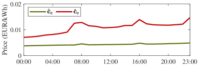
Figure 5: Flexibility cost coefficients of an aggregator.

In the following subsections, we solve the DSO flexibility market clearing model and analyze the activated flexibility of aggregators, the market settlement results, and the impact of the aggregator’s flexibility cost on the clearing results. We do not include a numerical comparison between the proposed market mechanism and that based on power adjustment ranges because the advantage of the proposed mechanism has been comprehensively discussed in Section II: power adjustment ranges do not adequately quantify the potential inconvenience caused to DER users by flexibility activation, thus failing to be used to formulate the corresponding flexibility costs.

V-B Results of the DSO Flexibility Market Clearing

In the flexibility market clearing, the input data of energy and reserve prices at the transmission level are real data from the Netherlands on Jan 2, 2024, where the energy price varied hourly with an average of 63.06 EUR/MWh, and the up- and down-reserve prices were constant and equal to 12.86 EUR/MW and 14.37 EUR/MW, respectively.

After solving the DSO flexibility market clearing model, the reference power profile and the power profiles corresponding to up- and down-reserves that the DSO offers to the transmission system are shown in Fig. 6. The reference power profile $\mathbf{P}_{0}^{\text{ref}}$ exhibits both upward and downward adjustments from the baseline $\mathbf{P}_{0}^{\text{base}}$, indicating that the DSO shifts the load for energy arbitrage. The gap between $\mathbf{P}_{0}^{\text{ru}}$ and $\mathbf{P}_{0}^{\text{rd}}$ represents reserve capacities. To be more precise, it is the down-reserve (i.e., increasing load), since $\mathbf{P}_{0}^{\text{ru}}$ coincides exactly with $\mathbf{P}_{0}^{\text{ref}}$. This coincidence can be explained as follows. Given $\mathbf{P}_{0}^{\text{ref}}=\mathbf{P}_{0}^{\text{ru}}$, then changing $\mathbf{P}_{0}^{\text{ref}}$ to be higher than $\mathbf{P}_{0}^{\text{ru}}$ (if feasible) will make 1) the flexibility cost remain unchanged, 2) the energy cost increase, 3) the revenue from down-reserve decrease, and 4) the revenue from up-reserve increase. Hence, changing $\mathbf{P}_{0}^{\text{ref}}$ to be higher than $\mathbf{P}_{0}^{\text{ru}}$ would not yield a better solution unless the increase in the revenue from up-reserve exceeds the decrease in the revenue from down-reserve plus the increase in energy cost. This condition, however, is not met in the tested case because the energy prices are significantly higher than the up-reserve prices.

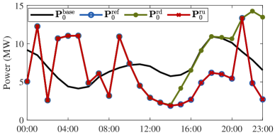
Figure 6: The baseline power profile $\mathbf{P}_{0}^{\text{base}}$, the reference power profile $\mathbf{P}_{0}^{\text{ref}}$ and power profiles corresponding to up- and down-reserves, $\mathbf{P}_{0}^{\text{ru}}$ and $\mathbf{P}_{0}^{\text{rd}}$, at the root node of the DSO.

We take the aggregator at node 2 as an example to illustrate the activated flexibility and the corresponding MFPs (see Fig. 7). The pattern of flexibility activation in Fig. 7, i.e., times and directions of the adjustments, is consistent with the adjustment pattern of power profiles at the root node from the baseline in Fig. 6. For instance, at 20:00, 22:00, and 23:00, $\mathbf{P}_{0}^{\text{ru}}$ and $\mathbf{P}_{0}^{\text{rd}}$ in Fig. 6 exhibit different adjustment directions relative to the baseline, which is reflected in Fig. 7(a), where both the upward and downward power adjustments at these times are nonzero, also correlating with the nonzero energy adjustments in Fig. 7(b) after 20:00. MFPs in Figs. 7(c) and 7(d) show the marginal contribution of power and energy adjustments to the DSO’s total revenue. While the power parts in the aggregator’s flexibility cost coefficients are all zero, the power part in MFP is nonzero because power adjustments contribute to the DSO’s total revenue.

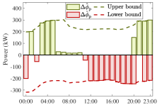
(a) Power adjustments

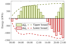
(b) Energy adjustments

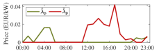
(c) MFPs for power

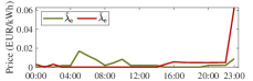
(d) MFPs for energy

Figure 7: The activated flexibility and MFPs. $\Delta\hat{\boldsymbol{\phi}}_{\text{p}}$ and $\Delta\check{\boldsymbol{\phi}}_{\text{p}}$: power parts of the flexibility trajectory’s upward and downward adjustment ranges; $\Delta\hat{\boldsymbol{\phi}}_{\text{e}}$ and $\Delta\check{\boldsymbol{\phi}}_{\text{e}}$: accumulated energy consumption parts of the flexibility trajectory’s upward and downward adjustment ranges; $\hat{\boldsymbol{\lambda}}_{\text{p}}$ and $\check{\boldsymbol{\lambda}}_{\text{p}}$: MFPs corresponding to the upward and downward power adjustment ranges; $\hat{\boldsymbol{\lambda}}_{\text{e}}$ and $\check{\boldsymbol{\lambda}}_{\text{e}}$: MFPs corresponding to the upward and downward adjustment ranges in accumulated energy consumption.

We next discuss the settlement results based on MFPs. First, we study the case without taking the voltage constraints into account, i.e. removing (20) from the problem formulation. In this case, the calculated total revenue of the DSO from energy arbitrage and reserve capacity provision in the transmission system, i.e., the left-hand side of inequality (30), is 4410.98 EUR. Distributing the revenues to each aggregator according to (29), the sum of each aggregator’s payment $R_{h}$, i.e., the right-hand side of inequality (30), is also 4410.98 EUR, exactly the same as the total revenue of the DSO. This result confirms that the proposed MFPs for settlement ensure the DSO’s balance of payments when the voltage constraints are not binding (equivalent to being absent). Then, by adding back the voltage constraints and studying a case where one of these constraints becomes binding, the DSO’s total revenue and the aggregators’ total payments are 4410.98 EUR and 4406.93 EUR, respectively, generating a surplus of 4.05 EUR. The surplus has been discussed right after Proposition 2.

V-C Impact of the Aggregators’ Flexibility Costs on the Market Clearing Results

This section analyzes the impact of the aggregators’ flexibility costs on the clearing results of the DSO’s flexibility market. First, the case where the flexibility costs of all aggregators change is tested. We multiply the cost coefficients of all aggregators by a parameter $\beta$ and analyze how the calculated total net cost and flexibility cost of the DSO change with $\beta$. The results, as shown in Fig. 8, indicate that as the flexibility cost coefficients increase, i.e., $\beta$ increases, the DSO’s total net cost also increases as expected. Second, the DSO’s overall flexibility cost initially increases and then decreases as the flexibility cost coefficients increase. This result is because the total flexibility cost is the product of the cost coefficients and the activated flexibility, and the latter decreases as the flexibility cost coefficients increase.

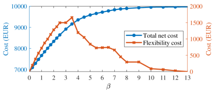
Figure 8: Changes in costs of the DSO with changes in the flexibility cost coefficients.

Next, we test the case where only the bidding cost coefficients of one aggregator change. It is assumed that the aggregators’ original cost coefficients are their true cost coefficients. Keeping the cost coefficients of other aggregators constant, we change the bidding cost coefficients of the aggregator at node 2 by multiplying it with the parameter $\beta$, implying that this aggregator does not bid its true cost coefficients. After the DSO flexibility market is cleared, the net profit of the aggregator (the received payment of the aggregator $R_{h}$ minus the aggregator’s true flexibility cost) can be obtained, as shown in Fig. 9. It is observed that the maximum net profit for the aggregator occurs at $\beta=1$, i.e., when the aggregator bids its true flexibility costs. This result verifies that the proposed market mechanism can encourage aggregators to report their true cost coefficients in a sufficiently competitive environment.

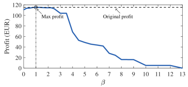
Figure 9: Changes in the profit of the aggregator at node 2 with its bidding flexibility cost.

VI Conclusions

This paper proposes a flexibility pricing method aligned with the flexibility models of DERs. For the flexibility of individual DERs, we propose to formulate its flexibility cost based on adjustment ranges in both power and accumulated energy consumption, which extends the traditional power range-based formulations. The proposed flexibility costs formulation quantifies the potential inconvenience caused to users of typical DERs such as EVs, DESS, and HPs by flexibility activation. We also propose a flexibility cost formulation aligned with the aggregated flexibility model and a DSO flexibility market model for activating flexibility to participate in the transmission system operation for energy arbitrage and reserve capacity provision. Furthermore, we propose the concept of MFPs for settlement, which ensures incentive compatibility, revenue adequacy, and a non-profit DSO. Numerical results validate the proposed pricing and market-clearing methods.

A potential limitation of this work lies in the calculation of the aggregators’ cost coefficients, which are estimated using a weighted average method in this paper and may be improved in future works. Future works can also focus on the coordination of the transmission system operation and the DSO flexibility market to better utilize flexibility to improve the operational efficiency of the entire power system.

Appendix A Proof of Proposition 1

We first reformulate the temperature evolution model (5) using a time-sequential form, as follows:

$${\theta_{T}}-\alpha{\theta_{T-1}} =(1-\alpha)(\theta_{T}^{{\text{amb}}}+\frac{\eta}{H}\cdot{p_{T}}),$$

$${\theta_{T-1}}-\alpha{\theta_{T-2}} =(1-\alpha)(\theta_{T-1}^{{\text{amb}}}+\frac{\eta}{H}\cdot{p_{T-1}}),$$

$$\cdots$$

$${\theta_{2}}-\alpha{\theta_{1}} =(1-\alpha)(\theta_{2}^{{\text{amb}}}+\frac{\eta}{H}\cdot{p_{2}}),$$

$${\theta_{1}}-\alpha{\theta_{0}} =(1-\alpha)(\theta_{1}^{{\text{amb}}}+\frac{\eta}{H}\cdot{p_{1}}),$$

where $\theta_{0}$ is the initial indoor temperature. These equations derive the relationship between the indoor temperature in the $t$-th time slot and the preceding power sequence $p_{1},p_{2},\cdots,p_{t}$:

$$\small{\theta_{t}}=(1-\alpha)\sum\limits_{\tau=1}^{t}{{\alpha^{t-\tau}}(\theta_{\tau}^{{\text{amb}}}+\frac{\eta}{H}\cdot{p_{\tau}})}+{\alpha^{t}}{\theta_{0}},\forall t\in[T].$$ (A.1)

Writing (A.1) in matrix form gives:

$$\boldsymbol{\theta}={\mathbf{A}}{\boldsymbol{\theta}^{{\text{amb}}}}+\frac{\eta}{H}\cdot{\mathbf{Ap}}+{\boldsymbol{\alpha}}{\theta_{0}},$$ (A.2)

where

$$\small{\mathbf{A}}\triangleq\left[{\begin{array}[]{cccc}1&{}\hfil&{}\hfil&{}\hfil\\ \alpha&1&{}\hfil&{}\hfil\\ \vdots&\ddots&\ddots&{}\hfil\\ {{\alpha^{T-1}}}&\cdots&\alpha&1\end{array}}\right],{\boldsymbol{\alpha}}\triangleq\left[{\begin{array}[]{c}\alpha\\ {{\alpha^{2}}}\\ \vdots\\ {{\alpha^{T}}}\end{array}}\right].$$

Equation (A.2) holds for the baseline power profile $\mathbf{p}^{\text{base}}$ and the temperature set point $\boldsymbol{\theta}^{\text{set}}$, that is:

$$\boldsymbol{\theta}^{\text{set}}={\mathbf{A}}{\boldsymbol{\theta}^{{\text{amb}}}}+\frac{\eta}{H}\cdot{\mathbf{Ap}^{\text{base}}}+{\boldsymbol{\alpha}}{\theta_{0}}.$$ (A.3)

Subtracting (A.3) from (A.2) yields:

$$\boldsymbol{\theta}-\boldsymbol{\theta}^{\text{set}}=\frac{\eta}{H}\cdot{\mathbf{A}(\mathbf{p}-\mathbf{p}^{\text{base}})}.$$ (A.4)

As the matrix $\mathbf{A}$ is invertible, namely its inverse is:

$$\small{{\mathbf{A}}^{-1}}=\left[{\begin{array}[]{cccc}1&{}\hfil&{}\hfil&{}\hfil\\ {-\alpha}&1&{}\hfil&{}\hfil\\ {}\hfil&\ddots&\ddots&{}\hfil\\ {}\hfil&{}\hfil&{-\alpha}&1\end{array}}\right],$$

expression (A.4) can be transformed to:

$${\mathbf{p}}-\mathbf{p}^{\text{base}}=\frac{H}{\eta}{{\mathbf{A}}^{-1}}\left({{\boldsymbol{\theta}}-\boldsymbol{\theta}^{\text{set}}}\right).$$ (A.5)

We now consider the temperature adjustment limits:

$$-\Delta\hat{\boldsymbol{\theta}}\leq\boldsymbol{\theta}-\boldsymbol{\theta}^{\text{set}}\leq\Delta\check{\boldsymbol{\theta}}.$$ (A.6)

This constraint cannot be transformed into power adjustment ranges in each time slot because the components of $\mathbf{A}^{-1}$ are not all positive, rendering the operation of multiplying both sides of inequality (A.6) by $\mathbf{A}^{-1}$ invalid. Therefore, we aim to establish a connection between the energy adjustment ranges $\Delta\hat{\mathbf{e}}$ and $\Delta\check{\mathbf{e}}$ and the temperature adjustment ranges $\Delta\hat{\boldsymbol{\theta}}$ and $\Delta\check{\boldsymbol{\theta}}$.

To this end, we first write the matrix form of the energy-power relationship (4):

$$\mathbf{e}=\Delta_{T}\mathbf{Lp},\mathbf{e}^{\text{base}}=\Delta_{T}\mathbf{Lp}^{\text{base}},$$ (A.7)

where $L$ is a $T\times T$ lower triangular matrix with all lower triangle elements equal to one. Multiplying both sides of (A.5) by $\Delta_{T}\mathbf{L}$ gives

$${\mathbf{e}}-\mathbf{e}^{\text{base}}=\Delta_{T}\cdot\frac{H}{\eta}{{\mathbf{LA}}^{-1}}\left({{\boldsymbol{\theta}}-\boldsymbol{\theta}^{\text{set}}}\right),$$ (A.8)

where

$$\small{\mathbf{L}}{{\mathbf{A}}^{-1}}=\left[{\begin{array}[]{cccc}1&{}\hfil&{}\hfil&{}\hfil\\ {1-\alpha}&1&{}\hfil&{}\hfil\\ \vdots&\ddots&\ddots&{}\hfil\\ {1-\alpha}&\cdots&{1-\alpha}&1\end{array}}\right].$$

All the components of ${\mathbf{L}}{{\mathbf{A}}^{-1}}$ are positive since $0<a<1$ by definition, hence it is feasible to multiply both sides of inequality (A.6) by $\Delta_{T}\cdot\frac{H}{\eta}{\mathbf{L}}{{\mathbf{A}}^{-1}}$ to derive the constraints on the energy adjustment ${\mathbf{e}}-\mathbf{e}^{\text{base}}$, i.e.,

$$-\Delta_{T}\cdot\frac{H}{\eta}{\mathbf{L}}{{\mathbf{A}}^{-1}}\Delta\hat{\boldsymbol{\theta}}\leq{\mathbf{e}}-\mathbf{e}^{\text{base}}\leq\Delta_{T}\cdot\frac{H}{\eta}{\mathbf{L}}{{\mathbf{A}}^{-1}}\Delta\check{\boldsymbol{\theta}}.$$ (A.9)

Let $\mathbf{D}\triangleq\Delta_{T}\cdot\frac{H}{\eta}{\mathbf{L}}{{\mathbf{A}}^{-1}}$, then $\Delta\hat{\mathbf{e}}={\mathbf{D}}\Delta\hat{\boldsymbol{\theta}}$ and $\Delta\check{\mathbf{e}}={\mathbf{D}}\Delta\check{\boldsymbol{\theta}}$, which complete the proof of Proposition 1.

References

- [1] IEA, “Status of Power System Transformation 2019,” International Energy Agency, Paris, 2019, accessed: 2024-02-17. [Online]. Available: https://www.iea.org/reports/status-of-power-system-transformation-2019
- [2] X. Jin, Q. Wu, and H. Jia, “Local flexibility markets: Literature review on concepts, models and clearing methods,” Applied Energy, vol. 261, p. 114387, 2020.
- [3] Ö. Okur, P. Heijnen, and Z. Lukszo, “Aggregator’s business models in residential and service sectors: A review of operational and financial aspects,” Renewable and Sustainable Energy Reviews, vol. 139, p. 110702, 2021.
- [4] M. Mousavi and M. Wu, “A DSO framework for market participation of DER aggregators in unbalanced distribution networks,” IEEE Transactions on Power Systems, vol. 37, no. 3, pp. 2247–2258, 2021.
- [5] M. Zhang, Y. Xu, and H. Sun, “Optimal coordinated operation for a distribution network with virtual power plants considering load shaping,” IEEE Transactions on Sustainable Energy, vol. 14, no. 1, pp. 550–562, 2022.
- [6] A. G. Givisiez, K. Petrou, and L. F. Ochoa, “A review on TSO-DSO coordination models and solution techniques,” Electric Power Systems Research, vol. 189, p. 106659, 2020.
- [7] V. Talaeizadeh, H. Shayanfar, and J. Aghaei, “Prioritization of transmission and distribution system operator collaboration for improved flexibility provision in energy markets,” International Journal of Electrical Power & Energy Systems, vol. 154, p. 109386, 2023.
- [8] N. Nazir and M. Almassalkhi, “Grid-aware aggregation and realtime disaggregation of distributed energy resources in radial networks,” IEEE Transactions on Power Systems, vol. 37, no. 3, pp. 1706–1717, 2021.
- [9] C. Ziras, J. Kazempour, E. C. Kara, H. W. Bindner, P. Pinson, and S. Kiliccote, “A mid-term dso market for capacity limits: How to estimate opportunity costs of aggregators?” IEEE Transactions on Smart Grid, vol. 11, no. 1, pp. 334–345, 2019.
- [10] X. Chen, E. Dall’Anese, C. Zhao, and N. Li, “Aggregate power flexibility in unbalanced distribution systems,” IEEE Transactions on Smart Grid, vol. 11, no. 1, pp. 258–269, 2019.
- [11] Z. Xu, D. S. Callaway, Z. Hu, and Y. Song, “Hierarchical coordination of heterogeneous flexible loads,” IEEE Transactions on Power Systems, vol. 31, no. 6, pp. 4206–4216, 2016.
- [12] L. Wang, J. Kwon, N. Schulz, and Z. Zhou, “Evaluation of aggregated EV flexibility with TSO-DSO coordination,” IEEE Transactions on Sustainable Energy, vol. 13, no. 4, pp. 2304–2315, 2022.
- [13] Z. Tan, H. Zhong, Q. Xia, C. Kang, X. S. Wang, and H. Tang, “Estimating the robust PQ capability of a technical virtual power plant under uncertainties,” IEEE Transactions on Power Systems, vol. 35, no. 6, pp. 4285–4296, 2020.
- [14] J. Jian, M. Zhang, Y. Xu, W. Tang, and S. He, “An analytical polytope approximation aggregation of electric vehicles considering uncertainty for the day-ahead distribution network dispatching,” IEEE Transactions on Sustainable Energy, 2023, early access.
- [15] Y. Wen, Z. Hu, S. You, and X. Duan, “Aggregate feasible region of DERs: Exact formulation and approximate models,” IEEE Transactions on Smart Grid, vol. 13, no. 6, pp. 4405–4423, 2022.
- [16] J. Liu, S. Y. Samson, H. Hu, J. Zhao, and H. M. Trinh, “Demand-side regulation provision of virtual power plants consisting of interconnected microgrids through double-stage double-layer optimization,” IEEE Transactions on Smart Grid, vol. 14, no. 3, pp. 1946–1957, 2022.
- [17] G. Tsaousoglou, J. S. Giraldo, P. Pinson, and N. G. Paterakis, “Mechanism design for fair and efficient DSO flexibility markets,” IEEE transactions on Smart Grid, vol. 12, no. 3, pp. 2249–2260, 2021.
- [18] T. Morstyn, A. Teytelboym, and M. D. McCulloch, “Designing decentralized markets for distribution system flexibility,” IEEE Transactions on Power Systems, vol. 34, no. 3, pp. 2128–2139, 2018.
- [19] J. Jian, P. Li, H. Ji, L. Bai, H. Yu, W. Xi, J. Wu, and C. Wang, “DLMP-based quantification and analysis method of operational flexibility in flexible distribution networks,” IEEE Transactions on Sustainable Energy, vol. 13, no. 4, pp. 2353–2369, 2022.
- [20] Z. You, S. D. Lumpp, M. Doepfert, P. Tzscheutschler, and C. Goebel, “Leveraging flexibility of residential heat pumps through local energy markets,” Applied Energy, vol. 355, p. 122269, 2024.
- [21] Y. Wen, Z. Hu, J. He, and Y. Guo, “Improved inner approximation for aggregating power flexibility in active distribution networks and its applications,” IEEE Transactions on Smart Grid, 2023, early access.
- [22] L. Bobo, L. Mitridati, J. A. Taylor, P. Pinson, and J. Kazempour, “Price-region bids in electricity markets,” European Journal of Operational Research, vol. 295, no. 3, pp. 1056–1073, 2021.