Temporal Entanglement Profiles in Dual-Unitary Clifford Circuits with Measurements

Abstract

We study temporal entanglement in dual-unitary Clifford circuits with probabilistic measurements preserving spatial unitarity. We exactly characterize the temporal entanglement barrier in the measurement-free regime, exhibiting ballistic growth and decay and a volume-law peak. In the presence of measurements, we show that the initial ballistic growth of temporal entanglement with bath size is modified to diffusive, which can be understood through a mapping to a persistent random walk model. The peak value of the temporal entanglement barrier exhibits volume-law scaling for all measurement rates. Additionally, measurements modify the ballistic decay to the “perfect dephaser limit” with vanishing temporal entanglement to an exponential decay, which we describe through a spatial transfer matrix method. The spatial dynamics is shown to be described by a non-Hermitian hopping model, exhibiting a PT-breaking transition at a critical measurement rate $p=1/2$.

I Introduction

Quantum circuit models recently emerged as a field of rapidly growing interest due to both experimental progress on noisy intermediate-scale quantum (NISQ) devices and newly-developed theoretical treatments. Experimentally, immense progress was made on realizing novel many-body quantum phases on quantum processors, such as topologically ordered states and time-crystalline eigenstate order [1, 2, 3]. Numerically, tensor-network based methods find natural applications in representing and simulating quantum circuits with built-in local structures, such as the brickwork or the staircase circuit geometries [4, 5, 6, 7]. Restricted classes of quantum circuits were additionally found to admit exact solvability, which allows for benchmarking of numerical and experimental results. One such example is the class of dual-unitary circuits, possessing unitarity along both the temporal and the spatial directions. Such circuits can act as minimal models for capturing a wide range of phenomena in many-body quantum dynamics [8, 9, 10, 11, 12, 13, 14]. On the one hand, unitarity in both space and time yields analytical solvability of such models; on the other, the constraint is loose enough to allow for generic behaviors ranging from integrable to chaotic dynamics [15, 9, 16, 12]. Besides these advances in methodology, quantum circuits present a natural setup for studying and observing new intriguing physical phenomena, with measurement-induced phase transitions as one of the paradigmatic examples [17, 18, 19, 20, 21, 22, 23, 24, 25, 26, 27]. These are new classes of nonequilibrium quantum phase transitions that manifest themselves in the entanglement scaling of the quantum systems of interest. Except for certain limiting cases, the universality classes of such transitions do not match any known classes, and immense effort is devoted to analytically characterizing the nature of such transitions.

For circuits with generic choice of gates, either originating from Trotterized Hamiltonian dynamics or directly representing Floquet unitary dynamics, exact results are generally out of reach, and matrix product state (MPS) evolution presents a natural choice of numerical method. In conventional approaches, one starts with the wave function represented as an MPS and updates it along the temporal direction by successively applying the appropriate unitary evolution operators [28, 29, 30, 31, 32, 33]. The numerical simulability of the system dynamics is determined by the scaling of the required bond dimension for storing the MPS wave function, which is physically governed by the growth of spatial entanglement [34, 35, 36].

An alternative approach dubbed the “folding algorithm” was proposed in Ref. [37], where one updates the time-evolved density matrix as a so-called “folded” MPS. In the folded representation, the density matrix $\rho$ is expressed as a wave function using the operator-state mapping: $\rho=|\Psi\rangle\langle\Psi|\rightarrow|\rho\rangle=|\Psi\rangle\otimes|\Psi\rangle^{*}$. The dynamics of this state follows as $|\rho(t)\rangle=(U\otimes U^{*})|\Psi_{0}\rangle\otimes|\Psi_{0}\rangle^{*}$. The trace operation, naturally appearing when calculating expectation values of observables, can be written as an inner product

$$\begin{split}\operatorname{tr}(\rho(t))\equiv\braket{\operatorname{tr}}{\rho(t)}=\bra{\operatorname{tr}}(U\otimes U^{*})|\Psi\rangle\otimes|\Psi\rangle^{*},\end{split}$$ (1)

where the first equation defines the inner product between a state vector and the “trace vector” $\bra{\operatorname{tr}}$.

The expectation value of a local observable $O$ can be expressed in the folded representation as

$$\begin{split}\langle O(t)\rangle&=\braket{\operatorname{tr}}{O}{\rho(t)}=\langle\operatorname{tr}|O(U\otimes U^{*})|\Psi\rangle\otimes|\Psi\rangle^{*}\\ &=\quad\vbox{\hbox{\includegraphics[width=216.81pt]{expectation_value.pdf}}}\end{split}$$ (2)

In the final equality we graphically represent the equation in the tensor network language (see e.g. Ref. [38]), making explicit the folding.

For a local observable $O$ supported on e.g. a single site, one could treat the spatial slice where $O$ acts nontrivially separately from the regions to its left and right, where it acts trivially. To do so, $\langle O(t)\rangle$ can be re-expressed as

$$\begin{split}\langle O(t)\rangle&=\langle I_{\text{left}}|\mathcal{T}_{O}|I_{\text{right}}\rangle\\ &=\quad\vbox{\hbox{\includegraphics[width=195.12767pt]{expectation_val2.pdf}}}\end{split}$$ (3)

For a spatially homogeneous evolution it is possible to identify a spatial transfer matrix such that the regions to the right and to the left can be written as powers of this matrix. Using $\langle I_{\text{left}}|$ as an example, in the folding algorithm, one starts with an arbitrary temporal MPS, $\langle\Phi|\otimes\langle\Phi|^{*}$, fixing the left boundary and successively applies to it the spatial transfer matrix $\mathcal{T}$. The thermodynamic limit of infinite system size can be taken by projecting $\langle\Phi|\otimes\langle\Phi|^{*}$ onto $\langle L|$, the dominant left eigenvector of $\mathcal{T}$:

$$\begin{split}\langle I_{\text{left}}|_{L\rightarrow\infty}&=\lim_{L\rightarrow\infty}\left(\left(\langle\Phi|\otimes\langle\Phi|^{*}\right)\mathcal{T}^{L}\right)\\ &=\lim_{L\rightarrow\infty}\quad\left(\vbox{\hbox{\includegraphics[width=216.81pt]{apply_transfer_matrix.pdf}}}\right)\\ &=\quad\vbox{\hbox{\includegraphics[width=52.03227pt]{left_FP.pdf}}}\quad=\langle L|\end{split}$$ (4)

Analogously, $|I_{\text{right}}\rangle_{L\rightarrow\infty}=\lim_{L\rightarrow\infty}\left(\mathcal{T}^{L}(|\Phi\rangle\otimes|\Phi\rangle^{*})\right)=|R\rangle$ is the dominant right eigenvector of $\mathcal{T}$.

Once these dominant eigenvectors are obtained, the value of $\langle O(t)\rangle$ in the thermodynamic limit can be computed as:

$$\begin{split}\lim_{L\rightarrow\infty}\langle O(t)\rangle=\quad\vbox{\hbox{\includegraphics[width=130.08731pt]{expect_val_FP.pdf}}}\end{split}$$ (5)

In the context of quenched dynamics, the folding algorithm typically allows for dynamical studies that can reach longer times than conventional methods. The numerical complexity is determined by the scaling of maximal entanglement of the temporal MPS’s $\langle I_{\text{left}}|$ and $|I_{\text{right}}\rangle$, dubbed the “temporal entanglement” [39, 40].

Using $\langle I_{\text{left}}|$ as example, the temporal entanglement $S_{T}$ is defined as

$$\begin{split}S_{T}=\max_{t_{i}=t_{1}\ldots t_{T-1}}S_{T}^{(t_{i})}\equiv\max_{t_{i}=t_{1}\ldots t_{T-1}}S_{\text{vN}}(\rho^{\langle I_{\text{left}}|}_{t_{i}})\end{split}$$ (6)

where $S_{\text{vN}}$ denotes the von Neumann entanglement entropy and $\rho^{\langle I_{\text{left}}|}_{t_{i}}$ is the reduced density matrix of $\langle I_{\text{left}}|$ with respect to the temporal bipartition at time $t_{i}$:

$$\begin{split}\rho^{\langle I_{\text{left}}|}_{t_{i}}=\quad\vbox{\hbox{\includegraphics[width=216.81pt]{reduced_density_matrix_IM.pdf}}}\end{split}$$ (7)

Analogous to the Feynman-Vernon influence functional [41], the vectorized tensors $\langle I_{\text{left}}|$ and $|I_{\text{right}}\rangle$ are dubbed “influence matrices” and interpreted as effective baths for the “impurity” $\mathcal{T}_{O}$ in Ref. [42]. Temporal entanglement therefore characterizes the memory effects, or non-Markovianity, of the effective bath.

Within the context of open quantum systems coupled to non-Markovian environments, an object analogous to the influence matrix was proposed and dubbed the “process tensor” [43, 44, 45]. The process tensor captures the effects of a non-Markovian environment and proves useful for studying the dynamics of open quantum system. In the context of the present work, however, the division between the subsystem and the environment is arbitrary due to the translational invariance of the system. The focus is therefore on the influence matrix, which encodes the dynamics of the closed quantum system, possibly subjected to measurements.

Various works were recently conducted on different aspects of the influence matrix and temporal entanglement. Areas of interest include the behavior of temporal entanglement for exactly solvable dynamics and dynamics close to integrability [46, 47, 48], using the influence matrix for treating quantum impurity problems [49, 50, 51], as well as using temporal entanglement as a way of characterizing generic quantum many-body dynamics [52].

Due to the action of tracing out these bath degrees of freedom at the end of the time evolution, or the “temporal boundary”, temporal entanglement generally displays behaviors different from its spatial counterpart. For instance, a system with spatial entanglement scaling as volume-law with system size might have temporal entanglement that scales as area-law with the total evolution time, and vice versa. A system which cannot be efficiently simulated along the temporal direction could admit a chance of being efficiently simulated along the spatial direction [40, 53, 54]. Observations as such motivate, from a numerical methodology point of view, study on the temporal entanglement scaling of (1+1) D quantum systems.

From a phenomenology perspective, temporal entanglement attracts interest in its own right, since it serves as a potential diagnostic for the nature of the quantum many-body dynamics. Depending on whether the system is free, interacting integrable, or chaotic, its temporal entanglement has been shown to display different scaling behaviors. With certain free systems admitting area-law temporal entanglement (TE) [55], certain interacting integrable systems admitting log-law TE [48], and generic chaotic systems admitting volume-law TE [52].

Despite growing interest in TE and its implication on the dynamics, analytical treatments of the TE at finite bath size – particularly its scaling with bath size – remains lacking. Such properties are relevant since 1) TE is known to not increase monotonously with bath size, but rather assumes a “barrier-like” shape [56]; it is the peak of the barrier, rather than the infinite-bath limit value of TE, that ultimately determines the numerical simulability of the dynamics; 2) without proper knowledge of the scaling of TE with bath size, or shape of the temporal entanglement barrier (TEB), convergence of the influence matrix (IM) to its thermodynamic-limit value may be difficult to determine; 3) the shape of the TEB carries additional information about the many-body dynamics that is not accessible from just the thermodynamic-limit value.

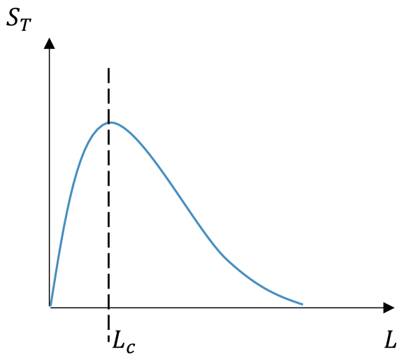
Figure 1: Schematic illustration of the temporal entanglement $S_{T}$ at different bath sizes $L$. $S_{T}$ does not increase monotonously with $L$ but rather assumes a barrier-like shape. The bath size corresponding to the peak of the barrier is dubbed the critical bath size, $L_{c}$.

The typical behavior of temporal entanglement with bath size is illustrated in Fig. 1, peaking at a critical bath size $L_{c}$. Furthermore, only systems with unitary dynamics have been studied so far, and TE in non-unitary systems, particularly monitored quantum circuits, have not yet been treated. Given the rapidly growing relevance of non-unitary quantum dynamics, it is natural to aim at developing a treatment for TE in non-unitary systems.

The present work fills the aforementioned two gaps: numerical and analytical characterizations are provided on the scaling of temporal entanglement with both total evolution time and bath size in quantum circuits with and without probabilistic measurements. The study is restricted to the class of dual-unitary Clifford circuits, with only measurements that preserve the spatial unitarity, in order to admit analytic results and allow for numerical simulations for large system sizes. Most results on the dynamics without measurements directly extends to generic dual-unitary circuits.

I.1 Outline of the Paper

This paper is structured as follows. Sec. II introduces the structure of the quantum circuits under study. Sec. III presents numerical and analytical results on temporal entanglement (TE) in circuits without measurements. Sec. IV presents numerical and analytical results on circuits with measurements, where the shape of the temporal entanglement barrier (TEB) is explained. Sec. V presents numerical and analytical results on a non-Hermitian phase transition with respective to the measurement rate. Sec. VI discusses the generality of the results beyond the simplest choice of SWAP gates, for which all derivations are particularly transparent. Conclusions are presented in Sec. VII.

I.2 Summary of Key Results

	$S_{T}$ growth	$S_{T}$ decay	$\lim_{L\rightarrow\infty}S_{T}$	$S_{T,\text{peak}}$	$L_{c}$
Unitary	$2L$	$T-L$	0	$2T/3$	$T/3$
Monitored	$\propto\sqrt{L}$	$\propto\exp{(-L/\xi)}$	0	$T/3$	$\propto T^{2}$

Table 1: Summary of Key Results. The variables in the entries are as follows: $S_{T}$ denotes temporal entanglement, $L$ denotes the bath size, and $T$ denotes the total evolution time. $\xi$ denotes some characteristic decay scale for $S_{T}$. $S_{T,\,\text{peak}}$ denotes the peak $S_{T}$ value, and $L_{c}$ denotes the critical bath size at which $S_{T,\,\text{peak}}$ is reached.

Table 1 summarizes key findings of this paper. Shapes of the temporal entanglement barrier (TEB) are characterized in dual-unitary Clifford circuits with and without measurements, dubbed “monitored” and “unitary” respectively. Upon introducing measurements, the initial growth of $S_{T}$ with $L$ changes from linear to diffusive, while the later decay of $S_{T}$ with $L$ changes from linear to exponential. The “steady-state” value of $S_{T}$ in the thermodynamic limit remains zero in both cases, and the peak $S_{T}$ value in the monitored setup is half of that in the unitary setup. The critical bath size $L_{c}$ at which $S_{T,\,\text{peak}}$ is reached scales quadratically with $T$ in the monitored case, to be contrasted with the linear scaling with $T$ in the unitary case.

II Quantum Circuit Setup

II.1 Brickwork Circuit Geometry

The quantum circuit of interest has the so-called “brickwork” geometry. The unitary evolution operators consists of alternating odd and even layers, with each layer consisting of tensor products of two-site unitary gates acting on odd and even bonds respectively:

$$\begin{split}U(T)&=\left(\prod_{i\>\text{odd}}U_{i,\,i+1}\prod_{i\>\text{even}}U_{i,\,i+1}\right)^{T}\\ &\text{}\\ &=\quad\vbox{\hbox{\includegraphics[width=238.49231pt]{evolution_U.pdf}}}\quad\ldots\end{split}$$ (8)

where $T$ is the total number of update steps for the Floquet evolution, which is henceforth referred to as the total evolution time. The building blocks of the full evolution operator are given by unitary matrices (gates) graphically represented as

$$\begin{split}U_{i,\,i+1}=\vbox{\hbox{\includegraphics[width=52.03227pt]{U_gate.pdf}}}\,.\end{split}$$ (9)

The brickwork geometry originates naturally from Trotterized Hamiltonian dynamics, where one alternates between switching on local interactions on all even bonds and all odd bonds, as is done in the Time-Evolving Block Decimation (TEBD) algorithm [32, 57].

For simplicity and analytic tractability, the initial state is chosen to be short-range entangled and takes the form:

$$\begin{split}|\Psi_{0}\rangle&=|\psi\rangle\otimes|\psi\rangle\otimes\ldots\otimes|\psi\rangle\\ &=\quad\vbox{\hbox{\includegraphics[width=195.12767pt]{Psi_0.pdf}}}\end{split}$$ (10)

where each two-site pair is denoted $|\psi\rangle$:

$$\begin{split}|\psi\rangle=\sum_{a,\,b}\psi_{ab}\,|a\rangle\otimes|b\rangle,\qquad\psi_{ab}=\;\vbox{\hbox{\includegraphics[width=52.03227pt]{little_psi.pdf}}}\,.\end{split}$$ (11)

Taken together, the time-evolved state in the folded picture under the brickwork circuit can be graphically denoted as:

$$\begin{split}&(U\otimes U^{*})|\Psi_{0}\rangle\otimes|\Psi_{0}\rangle^{*}\\ &\text{ }\\ =\quad&\vbox{\hbox{\includegraphics[width=238.49231pt]{evolved_Psi_new_untraced.pdf}}}\end{split}$$ (12)

For convenience, we use the same graphical notation for $U$ and $U^{*}$, with the implicit convention that all circuits in the top (bottom) layer correspond to $U$ ($U^{*}$). The trace operation is then applied at the end of the time evolution:

$$\begin{split}\langle I_{\text{left}}|=&\langle\operatorname{tr}|(U\otimes U^{*})|\Psi_{0}\rangle\otimes|\Psi_{0}\rangle^{*}\\ &\text{ }\\ =\quad&\vbox{\hbox{\includegraphics[width=238.49231pt]{evolved_Psi_new_traced.pdf}}}\end{split}$$ (13)

Following Ref. [42], the layer containing $U$ is dubbed the “forward time contour”, and the layer containing $U^{*}$ is dubbed the “backward time contour”.

We can identify a spatial transfer matrix $\mathcal{T}$ as:

$$\begin{split}&\text{}\\ &\mathcal{T}=\quad\vbox{\hbox{\includegraphics[width=86.72267pt]{spatial_transfer_matrix_new.pdf}}}\end{split}$$ (14)

II.2 Dual-Unitary and Clifford Gates

In this work we will restrict ourselves to dual-unitary Clifford gates. The two-site unitary gates appearing in the brickwork circuit can generally be any element of $U(4)$. Any choice of local unitary gates leads to global unitary time evolution, and we will refer to the unitarity as temporal unitarity. Graphically, this property reads:

$$\text{Temporal Unitarity}\quad\Leftrightarrow\quad\vbox{\hbox{\includegraphics[width=52.03227pt]{temporal_unitarity_new1.pdf}}}\quad=\quad\vbox{\hbox{\includegraphics[width=52.03227pt]{temporal_unitarity_new2.pdf}}}$$ (15)

Spatial unitarity can be analogously defined as:

$$\text{Spatial Unitarity}\quad\Leftrightarrow\quad\vbox{\hbox{\includegraphics[width=60.70653pt]{spatial_unitarity_new1.pdf}}}\quad=\quad\vbox{\hbox{\includegraphics[width=60.70653pt]{spatial_unitarity_new2.pdf}}}$$ (16)

Generally, a gate with temporal unitarity does not necessarily possess spatial unitarity. In the case where the gate possesses both, it is referred to as being “dual-unitary” [10, 8].

A general parametrization for two-site dual-unitary gates on qubits is given by [8]:

$$U=e^{i\phi}(u_{+}\otimes u_{-})V[J](v_{-}\otimes v_{+})\,,$$ (17)

where $\phi,\,J\in\mathbb{R}$, $u_{\pm},\,v_{\pm}\in SU(2)$, and the entangling gate defined as

$$V[J]=\exp\left[-i\left(\frac{\pi}{4}\sigma_{x}\otimes\sigma_{x}+\frac{\pi}{4}\sigma_{y}\otimes\sigma_{y}+J\sigma_{z}\otimes\sigma_{z}\right)\right]\,,$$ (18)

which is also known as the Trotterized XXZ gate. A brickwork circuit consisting of dual-unitary gates is itself dual-unitary.

The Clifford property refers to the fact that the gate can be generated from a specific set of gates, namely:

$$U_{\text{Clifford}}\in\langle\{H,S,\text{CNOT}\}\rangle$$ (19)

where, in the standard computational basis:

$$\begin{split}H=\frac{1}{\sqrt{2}}\begin{bmatrix}1&1\\ 1&-1\end{bmatrix},\quad S=\begin{bmatrix}1&0\\ 0&i\end{bmatrix},\quad\text{CNOT}=\begin{bmatrix}1&0&0&0\\ 0&1&0&0\\ 0&0&0&1\\ 0&0&1&0\end{bmatrix}.\end{split}$$ (20)

Up to single-site Clifford gates, there are two classes of two-site gates that are both dual-unitary and Clifford: the SWAP class and the iSWAP class. Brickwork circuits consisting of dual-unitary Clifford gates were previously studied in Ref. [58], where such nonrandom quantum circuits are dubbed “crystalline quantum circuits”.

The SWAP and the iSWAP gates corresponds to the Heisenberg and the XX points in the dual-unitary parameterization, respectively:

$$U_{\text{SWAP}}=V[J=\frac{\pi}{4}],\qquad U_{\text{iSWAP}}=V[J=0],$$ (21)

where $V[J]$ is defined in Eq. (18). In the present work, the SWAP gate and a variant in the iSWAP class are studied, namely the Clifford SDKI gate, or simply SDKI gate for brevity:

$$\begin{split}U_{\text{SDKI}}&=(H\otimes H)(S^{\dagger}\otimes S^{\dagger})U_{\text{iSWAP}}(H\otimes H)\\ &=CZ(H\otimes H)CZ\\ &=\quad\vbox{\hbox{\includegraphics[width=65.04034pt]{U_SDKI.pdf}}}\end{split}$$ (22)

The denomination of SDKIM originates from the use of this gate in the self-dual kicked Ising model. The generic kicked Ising model (KIM) is extensively studied in early works on dual-unitarity [59, 60], temporal entanglement [42, 56, 48] and emergent quantum state designs [61, 62]. The Clifford points, albeit being singular points in the continuous parameter space, admit efficient numerical simulability [63]. This motivates using the Clifford SDKI circuit alongside the SWAP circuit as toy models for investigating behavior of the temporal entanglement profile.

As pointed out in Ref. [64], the set of two-site dual-unitary Clifford gates makes up 50% of total two-site Clifford gates. The other two classes are the CNOT class and the identity class [65]. As such, the gate choice of being dual-unitary and Clifford is arguably not overly-constrained. While circuits consisting of CNOT gates are not dual-unitary, they are extensively studied in the contexts of the Floquet quantum East model [66, 67] as well as realizing generalized dual-unitary circuits [68]. Various recent works studied the entanglement membrane of such circuits [69, 70], with Ref. [71] focusing on generalized dual-unitary Clifford circuits.

II.3 Space-time Rotation, Significance of the Trace Operation and the Perfect-Dephaser Limit

The move from spatial entanglement to temporal entanglement fits within the larger frame of space-time rotation, exchanging the role of discrete time and discrete space in lattice circuit models [72, 73, 74, 64, 75]. After space-time rotation, a two-site unitary gate $U$ with matrix elements $U_{ab,cd}$ becomes a gate $\tilde{U}$ with matrix elements $\tilde{U}_{bd,ac}=U_{ab,cd}$:

$$\begin{split}U_{ab,cd}=\;\vbox{\hbox{\includegraphics[width=65.04034pt]{labeled_U_gate.pdf}}}\;\xrightarrow{\text{space-time rotation}}\;\tilde{U}_{bd,ac}=\vbox{\hbox{\includegraphics[width=65.04034pt]{labeled_U_gate2.pdf}}}\end{split}$$ (23)

Dual-unitary gates and dual-unitary circuits remain unitary after space-time rotation by construction.

The choice of initial state can possibly undermine the dual-unitarity of the circuit. For short-range entangled states as introduced in Eq. (10) and (11), unitarity along the spatial direction results in the condition $\sum_{j}\psi_{i,j}\psi^{*}_{k,j}=\delta_{ik}$, leading to so-called “solvable” initial states [14, 52], satisfying:

$$\begin{split}\vbox{\hbox{\includegraphics[width=86.72267pt]{solvable_init_new1.pdf}}}\quad=\quad\vbox{\hbox{\includegraphics[width=86.72267pt]{solvable_init_new2.pdf}}}\end{split}$$ (24)

By construction, such states possesses spatial unitarity. When contracted to a dual-unitary circuit, the contracted circuit remains unitary after space-time rotation.

Beyond short-range entangled states, solvability for generalized MPS initial states is discussed in Ref. [14]. For simplicity and in order to preserve the Clifford property, we choose $|\psi\rangle=(|00\rangle+|11\rangle)/\sqrt{2}\equiv|B_{I}\rangle$, such that:

$$\begin{split}\vbox{\hbox{\includegraphics[width=78.04842pt]{init_bell1.pdf}}}\quad=\quad\vbox{\hbox{\includegraphics[width=65.04034pt]{bell_pair1.pdf}}}\end{split}$$ (25)

Given the open boundary condition defined by the brickwork circuit structure in Eq. (8), the temporal MPS $\langle\Phi|$ at the spatial boundary consists of Bell-pair states connecting the site at time $t_{i}$ to the site at time $t_{i+1}$:

$$\begin{split}\langle\phi|\equiv\quad\vbox{\hbox{\includegraphics[width=43.36464pt]{phi1.pdf}}}\;,\quad\langle\Phi|=\langle\phi|\otimes\langle\phi|\otimes\ldots\otimes\langle\phi|=\;\vbox{\hbox{\includegraphics[width=34.69038pt]{boundary1.pdf}}}\end{split}$$ (26)

It will prove to be convenient to additionally define $\langle\theta|$ as a Bell pair connecting two equal-time sites at $t_{i}$ on the forward and backward time contours:

$$\langle\theta|\equiv\quad\vbox{\hbox{\includegraphics[width=52.03227pt]{PD_single_labeled.pdf}}}$$ (27)

After space-time rotation, each pair of trace operations becomes a projector $|\theta\rangle\langle\theta|$:

$$\begin{split}\vbox{\hbox{\includegraphics[width=86.72267pt]{trace_rotation.pdf}}}\quad\xrightarrow[\text{trace becomes projector}]{\text{space-time rotation}}\quad\vbox{\hbox{\includegraphics[width=86.72267pt]{trace_rotation2.pdf}}}\end{split}$$ (28)

Such projector is henceforth dubbed the “trace projector”.

Although dual-unitary gates and solvable initial conditions preserve spatial unitarity, the trace projector does not, rendering $\mathcal{T}$ non-unitary. Therefore, the behavior of temporal entanglement under update by $\mathcal{T}$ is generally different from the behavior of spatial entanglement under update by $U\otimes U^{*}$.

Ref. [42] pointed out that for dual-unitary circuits with solvable initial states the influence matrix $\langle I_{\text{left}}|$ always reduces to the so-called “perfect-dephaser” form for $L\geq T$, where $T$ is the total number of time steps of the Floquet evolution:

$$\langle I_{\text{PD}}|\equiv\langle\theta|\otimes\langle\theta|\otimes\ldots\otimes\langle\theta|=\;\vbox{\hbox{\includegraphics[width=43.36464pt]{PD1.pdf}}}$$ (29)

$$\langle I_{\text{PD}}|\mathcal{T}=\langle I_{\text{PD}}|$$ (30)

The perfect-dephaser influence matrix $\langle I_{\text{PD}}|$ has zero temporal entanglement, since temporal bipartitions would not cut across any Bell pairs. Therefore, dual-unitary circuit with solvable initial states always reaches zero temporal entanglement at system sizes $L\geq T$.

III Dual-Unitary Clifford Circuits without Measurement

This Section presents numerical and analytical results on temporal entanglement in dual-unitary Clifford circuits. The numerical results are obtained using the stabilizer formalism for simulating Clifford circuits [63, 17].

III.1 Numerical Results

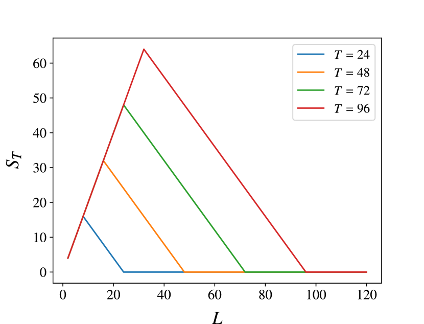
Figure 2: Temporal entanglement $S_{T}$ plotted against bath size $L$, with total evolution times $T=24,48,72,96$. Results are identical for either all-SWAP or all-SDKI circuits.

Fig. 2 shows the temporal entanglement as a function of the bath size $L$ at various total evolution times $T$. The gates are chosen to be SDKI, with the results for circuits with SWAP gates being identical. We can clearly identify three distinct regimes: an initial linear growth of temporal entanglement is followed by a linear decay, before saturating at a zero value. The overall function is piecewise linear and given by:

$$S_{T}(L)=\begin{cases}2L&\text{\; for\; }L<\frac{T}{3}\\ T-L&\text{\; for\; }\frac{T}{3}\leq L<T\\ 0&\text{\; for \; }L\geq T\end{cases}$$ (31)

Let us comment on some qualitative features. First, at $L=T/3$ and $L=T$, the TE changes non-analytically. This is because entanglement in Clifford circuits comes in the form of Bell pairs, and the number of Bell pairs across a given bipartition can only increase or decrease as integers. Second, temporal entanglement always decays to exactly zero for finite $L\geq T$. In this regime we recover the perfect dephaser limit [Eq. (29)], with $\langle I_{\text{left}}|=\langle I_{\text{PD}}|$ for $L\geq T$. Third, the peak TE scales linearly with the total evolution time $T$. Therefore, in the alternative order of limits where first $T\rightarrow\infty$ then $L\rightarrow\infty$ is taken, the TE would exhibit volume-law growth with $T$.

III.2 Analytical Derivation Through Diagrammatic Contractions

These different regimes and the corresponding TE can be analytically obtained using standard graphical manipulations. For stabilizer states, all orders of Rényi entropies are identical and equal the von Neumann entropy. We can hence focus on the second Rényi entropy, since it requires the smallest tensor power of $\langle I_{\text{left}}|$:

$$S_{T}^{(t_{i})} =S_{\text{vN}}\left(\rho_{t_{i}}^{\langle I_{\text{left}}|}\right)=-\log_{2}\frac{\operatorname{tr}\left(\left(\rho_{t_{i}}^{\langle I_{\text{left}}|}\right)^{2}\right)}{\operatorname{tr}\left(\left(\rho^{\langle I_{\text{left}}|}\right)^{2}\right)}$$

$$\equiv-\log_{2}D_{t_{i}}^{\langle I_{\text{left}}|},$$ (32)

where $D_{t_{i}}^{\langle I_{\text{left}}|}$ is the purity with respect to bipartition at $t_{i}$.

Using the operator-state mapping, one may write $\rho^{\bra{I_{\text{left}}}}$ as:

$$\begin{split}\rho^{\langle I_{\text{left}}|}=|I_{\text{left}}\rangle\langle I_{\text{left}}|\rightarrow|\rho^{\langle I_{\text{left}}|}\rangle\equiv|I_{\text{left}}\rangle\otimes|I_{\text{left}}\rangle^{*}\,.\end{split}$$ (33)

Since each $|I_{\text{left}}\rangle$ contains a layer of $U$ and $U^{*}$ each, $\left(\rho^{\langle I_{\text{left}}|}\right)^{\otimes 2}$ contains 4 layers of $U$ and $U^{*}$ each, and we can write:

$$\begin{split}\left(\rho^{\langle I_{\text{left}}|}\right)^{\otimes 2}&=\quad\vbox{\hbox{\includegraphics[width=216.81pt]{eight_layers_new.pdf}}}\end{split}$$ (34)

Note that the graphical representation circuit is rotated w.r.t. its original representation [Eq. (13)], corresponding to a space-time rotation.

It is convenient to define a new merged representation, where:

$$\begin{split}\vbox{\hbox{\includegraphics[width=52.03227pt]{merged_gate1.pdf}}}\quad\equiv\quad\vbox{\hbox{\includegraphics[width=121.41306pt]{merged_gate2_new.pdf}}}\end{split}$$ (35)

These gates are operators acting on pairs of 8 copies of the local Hilbert space. The contraction order associated with the trace projector is denoted by a triangle:

$$\begin{split}\vbox{\hbox{\includegraphics[width=65.04034pt]{merged_gate3.pdf}}}\;\equiv\quad\vbox{\hbox{\includegraphics[width=86.72267pt]{merged_gate4_new.pdf}}}\quad,\quad\vbox{\hbox{\includegraphics[width=21.68231pt]{triangle_single_vertical.pdf}}}\;\equiv\;\vbox{\hbox{\includegraphics[width=86.72267pt]{triangle_bracket.pdf}}}\end{split}$$ (36)

corresponding to a state in 8 copies of the local Hilbert space. All necessary contractions for our calculation can be similarly represented, where two additional contraction orders appear on the two sides of the bipartition:

$$\begin{split}\vbox{\hbox{\includegraphics[width=65.04034pt]{contract_order1.pdf}}}\quad&\equiv\quad\vbox{\hbox{\includegraphics[width=86.72267pt]{contract_order2_new.pdf}}}\quad,\quad\vbox{\hbox{\includegraphics[width=17.34189pt]{circle_single.pdf}}}\;\equiv\;\vbox{\hbox{\includegraphics[width=86.72267pt]{circle_bracket.pdf}}}\\ \vbox{\hbox{\includegraphics[width=65.04034pt]{contract_order3.pdf}}}\quad&\equiv\quad\vbox{\hbox{\includegraphics[width=86.72267pt]{contract_order4_new.pdf}}}\quad,\quad\vbox{\hbox{\includegraphics[width=13.00806pt]{square_single.pdf}}}\;\equiv\;\vbox{\hbox{\includegraphics[width=86.72267pt]{square_bracket.pdf}}}\end{split}$$ (37)

Temporal and spatial unitarity lead to a set of graphical identities allowing specific boundary vectors to propagate through the system:

$$\begin{split}\vbox{\hbox{\includegraphics[width=60.70653pt]{contract_rules5.pdf}}}\;=\;\vbox{\hbox{\includegraphics[width=60.70653pt]{contract_rules6.pdf}}}\;,\quad\vbox{\hbox{\includegraphics[width=52.03227pt]{contract_rules7.pdf}}}\;=\;\vbox{\hbox{\includegraphics[width=52.03227pt]{contract_rules8.pdf}}}\end{split}$$ (38)

and similarly for the circles and the squares in Eq. (37).

Let us illustrate how these contractions appear in a simple example. We consider a circuit with $L=4$, $T=8$ and calculate the TE for a bipartition across $t_{i}=t_{1}$. The Rényi entropy (III.2) requires evaluating the following two diagrams:

$$\begin{split}\operatorname{tr}\left(\left(\rho_{t_{i}}^{\langle I_{\text{left}}|}\right)^{2}\right)&=\;\vbox{\hbox{\includegraphics[width=281.85034pt]{purity1_new.pdf}}}\\ \operatorname{tr}\left(\left(\rho^{\langle I_{\text{left}}|}\right)^{2}\right)&=\;\vbox{\hbox{\includegraphics[width=281.85034pt]{purity2_new.pdf}}}\end{split}$$ (39)

Using the graphical identities (38), contracting the diagram requires evaluating the overlap between the different boundary vectors representing different contraction orders. These overlaps correspond to counting the number of loops, with each contracted loop contributing a factor of $q=2$ to the overall purity calculation, where $q$ is the local Hilbert space dimension:

$$\vbox{\hbox{\includegraphics[width=43.36464pt]{loop1.pdf}}}\quad=2,$$ (40)

leading to, e.g.,

$$\begin{split}\vbox{\hbox{\includegraphics[width=43.36464pt]{circle_square_bell.pdf}}}\quad=\quad\vbox{\hbox{\includegraphics[width=43.36464pt]{circle_square_loops_new.pdf}}}\quad=2^{2}=4.\end{split}$$ (41)

The required overlaps follow as

$$\begin{split}\vbox{\hbox{\includegraphics[width=43.36464pt]{triangle_circle.pdf}}}\quad&=\quad\vbox{\hbox{\includegraphics[width=43.36464pt]{triangle_square.pdf}}}\quad=\;2^{2},\\ \vbox{\hbox{\includegraphics[width=43.36464pt]{triangle1.pdf}}}\quad&=\quad\vbox{\hbox{\includegraphics[width=43.36464pt]{circle1.pdf}}}\quad=\quad\vbox{\hbox{\includegraphics[width=43.36464pt]{square1.pdf}}}\quad=\;2^{4}.\end{split}$$ (42)

Using spatial unitarity to contract vertically yields:

$$\begin{split}\operatorname{tr}\left(\left(\rho_{t_{i}}^{\langle I_{\text{left}}|}\right)^{2}\right)&=\;\vbox{\hbox{\includegraphics[width=281.85034pt]{simplify_vertical1.pdf}}}\end{split}$$ (43)

This diagram can now be further simplified using temporal unitarity to contract horizontally, resulting in:

$$\begin{split}\operatorname{tr}\left(\left(\rho_{t_{i}}^{\langle I_{\text{left}}|}\right)^{2}\right)&=\;\vbox{\hbox{\includegraphics[width=281.85034pt]{simplify_horizontal1.pdf}}}\\ &=\;\left(\vbox{\hbox{\includegraphics[width=43.36464pt]{triangle_circle.pdf}}}\right)^{3}\left(\vbox{\hbox{\includegraphics[width=43.36464pt]{circle1.pdf}}}\right)^{1}\left(\vbox{\hbox{\includegraphics[width=43.36464pt]{circle_square_bell.pdf}}}\right)^{2}=2^{14}\end{split}$$ (44)

An analogous calculation holds for $\operatorname{tr}\left(\left(\rho^{\langle I_{\text{left}}|}\right)^{2}\right)$:

$$\begin{split}\operatorname{tr}\left(\left(\rho^{\langle I_{\text{left}}|}\right)^{2}\right)=\;\left(\vbox{\hbox{\includegraphics[width=43.36464pt]{triangle_square.pdf}}}\right)^{3}\left(\vbox{\hbox{\includegraphics[width=43.36464pt]{square1.pdf}}}\right)^{3}=2^{18},\end{split}$$ (45)

resulting in $D^{\langle I_{\text{left}}|}_{t_{i}}=2^{-4}$ and $S_{2}\left(\rho^{\langle I_{\text{left}}|}_{t_{i}}\right)=2$.

Upon normalization, only connections between a circle and a square contributes to the purity, and each such connection contributes a factor of $2^{-2}$. Therefore,

$$S_{T}^{(t_{i})}=2\times\text{Number of}\;\left(\vbox{\hbox{\includegraphics[width=43.36464pt]{circle_square_bell.pdf}}}\right)\;\equiv 2\cdot n_{\text{cs}},$$ (46)

where $n_{\text{cs}}$ is the number of circle-square pairs. This result admits a direct interpretation: physically, each Bell pair crossing the boundary of the bipartition contributes one unit of $S_{T}^{(t_{i})}$. Since each $\langle I_{\text{left}}|$ contains both the forward and the backward time contours, each connection between a circle and a square represents two Bell pairs crossing the boundary and contributes two units of $S_{T}^{(t_{i})}$.

After dropping trivial pairings, different classes of diagrams can occur depending on the values of $L$, $T$, and $t_{i}$. Each parameter regime is now discussed separately.

III.2.1 Regime 1: $0<L<T/3$

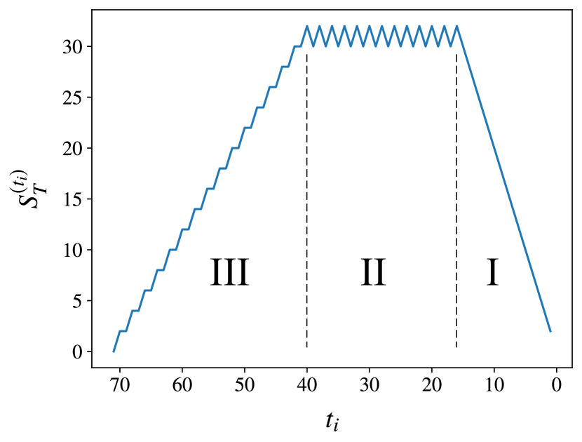
Figure 3: Temporal entanglement plotted against temporal bipartition point $t_{i}$, with total evolution time $T=72$ and bath size $L=16$. There are 3 bipartition intervals, each showing different phenomenologies. Interval I is $0<t_{i}<L$, Interval II is $L\leq t_{i}<T-2L$, and Interval III is $T-2L\leq t_{i}<T$.

We will first consider the regime where the bath size $L$ is small compared to the total time evolution $T$, more specifically with $0<L<T/3$. The temporal entanglement profile for this regime is shown in Fig. 3. The three intervals of bipartition location $t_{i}$ are now analyzed separately. To avoid even-odd parity effects, $t_{i}$ is chosen to be always odd.

The first bipartition interval is $0<t_{i}<L$. There, the contracted diagram is of the shape:

$$\begin{split}\vbox{\hbox{\includegraphics[width=173.44534pt]{topo1.pdf}}}\;=\;\vbox{\hbox{\includegraphics[width=173.44534pt]{topo1_contract.pdf}}}\end{split}$$ (47)

All circle contractions can be propagated from the left, leading to a number of circle-square pair $n_{\text{cs}}=t_{i}$. In this interval, all legs between $t=0$ and $t=t_{i}$ are paired up with legs from the other bipartition. Therefore, the number of Bell pairs crossing the bipartition increases linearly with $t_{i}$, with slope 1 per time contour. This result indicates a maximal TE bounded only by the size of the bipartition: due to the small bath size in this regime all information that initially “leaks” into the bath will strongly influence future dynamics.

The second bipartition interval is $L\leq t_{i}<T-2L$. There, the contracted diagram is of the shape:

$$\begin{split}\vbox{\hbox{\includegraphics[width=195.12767pt]{topo2.pdf}}}\;=\;\vbox{\hbox{\includegraphics[width=195.12767pt]{topo2_contract.pdf}}}\end{split}$$ (48)

Here the contractions can be propagated either from the left or to the right. In this interval, $n_{\text{cs}}=L$ independent of $t_{i}$, and the number of contributing Bell pairs is limited by $L$ and therefore insensitive to the precise location of the bipartition. The TE has effectively saturated at a maximal value bounded by the bath size, behaving strongly non-Markovian.

The last bipartition interval is $T-2L<t_{i}<T$. Here, the contracted diagram is of the shape:

$$\begin{split}\vbox{\hbox{\includegraphics[width=195.12767pt]{topo3.pdf}}}\;=\;\vbox{\hbox{\includegraphics[width=195.12767pt]{topo3_contract.pdf}}}\end{split}$$ (49)

In this interval $n_{\text{cs}}=(T-t_{i})/2$, the number of Bell pairs annihilated by the trace projectors increases linearly with $t_{i}$, with slope $1/2$. The slope accounts for the fact that for every increment of $t_{i}$ by 2, two additional Bell pairs per time contour cross the bipartition, similar to the diagrams of Eq. (47). However, due to the trace operator, one contributing Bell pair from each time contour is annihilated, and some information that enters the bath is no longer accessible. The different boundaries in time (initial state vs. trace operator) hence introduce an asymmetry between the short-time and late-time bipartitions.

The analysis for the three intervals of this regime matches the profile shown in Fig. 3. The choice of bipartition $t_{i}$ that maximizes the entanglement entropy is then anywhere within the interval $L\leq t_{i}\leq T-2L$. The corresponding temporal entanglement follows as $S_{T}=2\cdot\text{max}_{t_{i}}(n_{\text{cs}})=2L$.

III.2.2 Regime 2: $T/3\leq L<T/2$

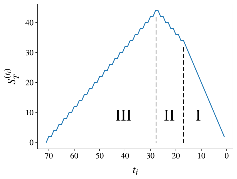
Figure 4: Temporal entanglement plotted against temporal bipartition point $t_{i}$, with total evolution time $T=72$ and bath size $L=28$. There are 3 bipartition intervals, each showing different phenomenologies. Interval I is $0<t_{i}<T-2L$, Interval II is $T-2L\leq t_{i}<L$, and Interval III is $L\leq t_{i}<T$.

Next, we consider the regime where the size of the bath is larger than $T/3$ but smaller than half the total time evolution $T/2$, such that Bell pairs propagating ballistically through the bath can hit the boundary and return, and memory effects are hence expected to play a role here. The temporal entanglement profile for this regime is shown in Fig. 4. The three intervals of the bipartition location $t_{i}$ are again analyzed separately. To avoid even-odd site effects, $t_{i}$ is again chosen to be always odd.

The first bipartition interval is $0<t_{i}<T-2L$. There, the contracted diagram have the shape of Eq. (47), and $n_{\text{cs}}=t_{i}$. The phenomenology is the same as the one for the first interval in Regime 1.

The second bipartition interval is $T-2L\leq t_{i}<L$. There, the contracted diagram is of the shape:

$$\begin{split}\vbox{\hbox{\includegraphics[width=216.81pt]{topo4.pdf}}}\end{split}$$ (50)

where

$$\begin{split}L<\frac{T}{2}\;\Rightarrow\;\#\left(\;\vbox{\hbox{\includegraphics[width=21.68231pt]{triangle_single.pdf}}}\;\right)-\#\left(\;\vbox{\hbox{\includegraphics[width=8.67424pt]{square_single.pdf}}}\;\right)=L-\frac{T-t_{i}}{2}-t_{i}<0.\end{split}$$ (51)

While all results so far held for general dual-unitary circuits, the diagram (50) cannot be further simplified using dual-unitarity alone. However, the SWAP gate and the SDKI gate both possess the additional symmetries of being self-dual and real:

$$\begin{split}\vbox{\hbox{\includegraphics[width=43.36464pt]{merged_gate1_original.pdf}}}\quad=\quad\vbox{\hbox{\includegraphics[width=43.36464pt]{merged_gate1.pdf}}},\qquad\vbox{\hbox{\includegraphics[width=43.36464pt]{merged_gate1_original.pdf}}}\quad=\quad\left(\;\vbox{\hbox{\includegraphics[width=43.36464pt]{merged_gate1_original.pdf}}}\;\right)^{*}\,.\end{split}$$ (52)

Therefore, if the circuit consists solely of SWAP or solely of SDKI gates, exactly the Clifford gates under consideration, the following identity holds:

$$\begin{split}\vbox{\hbox{\includegraphics[width=78.04842pt]{corner1.pdf}}}\;=\;\vbox{\hbox{\includegraphics[width=78.04842pt]{corner2.pdf}}}\end{split}$$ (53)

Using Eq. (53) the diagram (50) can be further simplified, and $n_{\text{cs}}=t_{i}/2-L+T/2$:

$$\begin{split}\vbox{\hbox{\includegraphics[width=195.12767pt]{topo4.pdf}}}\;=\vbox{\hbox{\includegraphics[width=195.12767pt]{topo4_contract.pdf}}}\end{split}$$ (54)

In this interval, effects from both temporal boundaries need to be taken into account: the number of contributing Bell pairs increases linearly with $t_{i}$ with slope 1 per time contour, while the number of Bell pairs annihilated by the trace projectors also increases linearly with $t_{i}$ with slope $1/2$ per time contour. Therefore, the net increase in number of contributing Bell pairs is linear in $t_{i}$ with slope $1/2$. In the generic case where Eq. (53) does not hold, the temporal entanglement profiles of these diagrams are different, as is discussed in Appendix A.

The third bipartition interval is $L\leq t_{i}<T$. There, the contracted diagram has the shape of Eq. (49), and $n_{\text{cs}}=(T-t_{i})/2$. The phenomenology is the same as the one for the third interval in Regime 1.

The analysis for the three intervals of Regime 2 matches the profile shown in Fig. 4. The $t_{i}$ for maximal entanglement entropy is at $t_{i}=L$. The corresponding temporal entanglement is $S_{T}=2\cdot\text{max}_{t_{i}}(n_{\text{cs}})=T-L$.

III.2.3 Regime 3: $T/2\leq L<T$

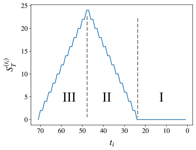
Figure 5: Temporal entanglement plotted against temporal bipartition point $t_{i}$, with total evolution time $T=72$ and bath size $L=48$. There are 3 bipartition intervals, each showing different phenomenologies. Interval I is $0<t_{i}<2L-T$, Interval II is $2L-T\leq t_{i}<L$, and Interval III is $L\leq t_{i}<T$.

Let us now consider the limit where the bath size is on the same order as the total evolution time, but constrained to $L\geq T/2$ such that ballistically propagating Bell pairs can not traverse the length of the bath twice and the right boundary is hence expected to not play a role. The temporal entanglement profile for Regime 3 is shown in Fig. 5. There are again three intervals of bipartition location $t_{i}$, with $t_{i}$ again chosen to be always odd.

The first bipartition interval is $0<t_{i}<2L-T$. There, the contracted diagram is of the shape:

$$\begin{split}\vbox{\hbox{\includegraphics[width=216.81pt]{topo4b.pdf}}}\end{split}$$ (55)

where

$$\begin{split}&L>\frac{T}{2},\,t_{i}<2L-T\;\\ &\Rightarrow\;\#\left(\;\vbox{\hbox{\includegraphics[width=21.68231pt]{triangle_single.pdf}}}\;\right)-\#\left(\;\vbox{\hbox{\includegraphics[width=8.67424pt]{square_single.pdf}}}\;\right)=L-\frac{T-t_{i}}{2}-t_{i}>0.\end{split}$$ (56)

Similar to the diagrams of Eq. (50), these cannot be further simplified using dual-unitarity alone. For all-SWAP or all-SDKI circuits, Eq. (53) again holds, and $n_{\text{cs}}=0$ independent of $t_{i}$:

$$\begin{split}\vbox{\hbox{\includegraphics[width=195.12767pt]{topo4b.pdf}}}\;=\;\vbox{\hbox{\includegraphics[width=195.12767pt]{topo4b_contract.pdf}}}\end{split}$$ (57)

In this interval, all Bell pairs available for cross-bipartition pairing are connected to trace projectors, and no contributing Bell pairs remain. For these bipartitions the TE vanishes and the bath can be treated as a purely Markovian perfect dephaser. Numerical results on these diagrams for generic dual-unitary Clifford circuits are presented in Appendix A.

The second bipartition interval is $2L-T\leq t_{i}<L$. There, the contracted diagram has the shape of Eq. (50), and $n_{\text{cs}}=t_{i}/2-L+T/2$. The phenomenology is the same as the one for the second interval of Regime 2. The third bipartition interval is $L\leq t_{i}<T$. There, the contracted diagram has the shape of Eq. (49), and $n_{\text{cs}}=(T-t_{i})/2$. The phenomenology is the same as the one for the third interval of Regime 1 and 2.

The analysis for the three intervals of Regime 3 matches the profile shown in Fig. 5. The $t_{i}$ for maximal entanglement entropy is at $t_{i}=L$. The corresponding temporal entanglement follows as $S_{T}=2\cdot\text{max}_{t_{i}}(n_{\text{cs}})=T-L$.

III.2.4 Regime 4: $L\geq T$

We now consider the final limit where the bath size is larger than the number of discrete time steps. In Regime 4, the contracted diagram always takes on the following shape:

$$\begin{split}\vbox{\hbox{\includegraphics[width=108.405pt]{topo5.pdf}}}\quad=\quad\vbox{\hbox{\includegraphics[width=108.405pt]{topo5_contract.pdf}}}\end{split}$$ (58)

In these diagrams $n_{\text{cs}}=0$ independent of $t_{i}$. All Bell pairs available for cross-bipartition pairing are connected to trace projectors. Therefore in this regime $S_{T}=0$ always, and the bath reduces to the expected perfect dephaser limit.

These results exhaust the possible temporal entanglement profiles, and match with the piecewise linear form presented in Eq. (31). The linear profile can be intuitively understood through the ballistic dynamics of the (ends of the) Bell pairs. E.g., the initial growth of temporal entanglement with each update step can be understood by noting that the boundary Bell pairs spread ballistically under the action of the dual-unitary circuit, and the radius of each Bell pair grows linearly with each spatial update step. Since the update preserves the center of mass of each Bell pair, the number of Bell pairs crossing the optimal temporal bipartition site also grows linearly with each update step. In other regimes the obtained linear profile follows by additionally taking into account reflection at the spatial boundary and absorption due to the trace at the temporal boundary.

IV Circuits with Probabilistic Measurements

Let us now consider the effect of projective measurements on the dynamics of the TE. In order to preserve the spatial unitarity and the Clifford nature of the dynamics, we restrict ourselves to measurements in the Bell-pair basis. The resulting TE profile is derived and we provide a mapping to a persistent random walk model for the resulting diffusive growth dynamics.

IV.1 Measurements Preserving Spatial Unitarity

We focus on two-site measurements in the Bell-pair basis, also known as unitary-error-basis (UEB) measurements [76]. There are four basis states for two qubits, denoted by:

$$|B_{I}\rangle =(|00\rangle+|11\rangle)/\sqrt{2},\quad|B_{X}\rangle=(|01\rangle+|10\rangle)/\sqrt{2},$$ (59)

$$|B_{Y}\rangle =(|01\rangle-|10\rangle)/\sqrt{2},\quad|B_{Z}\rangle=(|00\rangle-|11\rangle)/\sqrt{2}.$$ (60)

The Bell-pair measurements break temporal unitarity while preserving spatial unitarity for any measurement outcome [14, 77, 78, 79, 80]. Therefore, the spatial transfer matrix remains unitary upon adding measurements. Upon space-time rotation, projectors onto the four basis states map to (unitary) products of single-site Pauli operators:

$$|B_{I}\rangle\langle B_{I}| \rightarrow\mathds{1}\otimes\mathds{1}, \qquad|B_{X}\rangle\langle B_{X}|\rightarrow\sigma_{x}\otimes\sigma_{x},$$ (61)

$$|B_{Y}\rangle\langle B_{Y}| \rightarrow\sigma_{y}\otimes\sigma_{y}, \qquad|B_{Z}\rangle\langle B_{Z}|\rightarrow\sigma_{z}\otimes\sigma_{z}.$$ (62)

Graphically, for $\alpha\in\{I,X,Y,Z\}$ we can write that:

$$\vbox{\hbox{\includegraphics[width=65.04034pt]{bell_meas.pdf}}}\quad\xrightarrow{\text{space-time rotation}}\quad\vbox{\hbox{\includegraphics[width=65.04034pt]{bell_meas_rotated.pdf}}}$$ (63)

In a true measurement, the outcome of having one of the four basis states is probabilistic, with the probability given by the Born rule. Viewed spatially, the different outcomes correspond to applications of different Pauli operators. Since Pauli operators only incur a potential sign-change on the stabilizers, they do not change the entanglement structure of the state [63]. Therefore, without loss of generality, the present work replaces each true measurement by the projector $|B_{I}\rangle\langle B_{I}|$, such that the two qubits are forced to be in the $|B_{I}\rangle$ state after the measurement. This protocol is also known as the “forced measurement” or “post-selected measurement” protocol [64, 81, 82, 73].

Each two-site unitary gate in the circuit has a probability $p$ of being replaced by a forced measurement. This random choice is made independently among all gates. Once the gate at sites $i$, $i+1$ and times $t_{i}$, $t_{i+1}$ along the forward time contour is chosen to be replaced by a measurement, the same choice must be made for the gate at the corresponding sites and times on the backward time contour, since the time evolution operator is identical between the two time contours for any chosen stochastic trajectory. In the folded representation, the measurement outcomes are referred to as being “locked” among all layers.

Graphically,

$$\begin{split}\vbox{\hbox{\includegraphics[width=43.36464pt]{prob_unitary.pdf}}}=\;\begin{cases}\quad\vbox{\hbox{\includegraphics[width=43.36464pt]{merged_gate1_original.pdf}}}\quad&\text{with probability $1-p$,}\\ &\text{}\\ \quad\vbox{\hbox{\includegraphics[width=43.36464pt]{projector.pdf}}}\quad&\text{with probability $p$,}\end{cases}\end{split}$$ (64)

where the gates are already in the merged representation.

IV.2 Numerical Results with Measurements

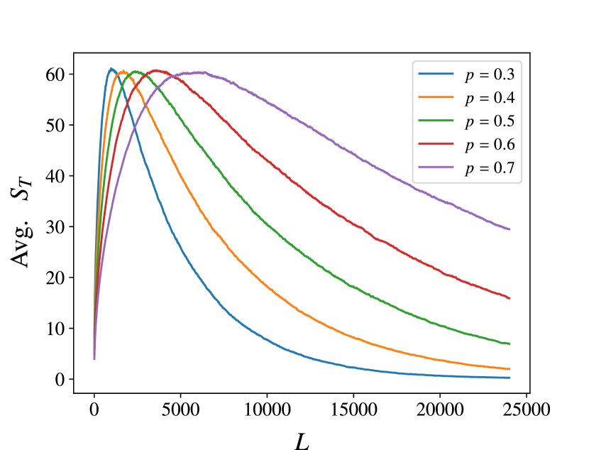
Figure 6: Average temporal entanglement $S_{T}$ plotted against bath size $L$ for total evolution time $T=216$ and different measurement rates $p$.

Fig. 6 shows the temporal entanglement as a function of the bath size for a fixed evolution time $T$ and varying measurement rates. Introducing measurements induces a few qualitative changes as compared to the case of unitary circuits without measurements. For the growth regime we find that:

$$S_{T}\propto L,\;p=0\quad\rightarrow\quad S_{T}\propto\sqrt{L},\;0<p<1,$$ (65)

whereas for the decay regime:

$$S_{T}\propto\textrm{Cst.}-L,\;p=0\quad\rightarrow\quad S_{T}\propto\exp{(-L/\xi)},\;0<p<1,$$ (66)

where the characteristic scale $\xi$ increases with $p$. The linear growth and decay of TE is replaced by a diffusive growth and an exponential decay, respectively.

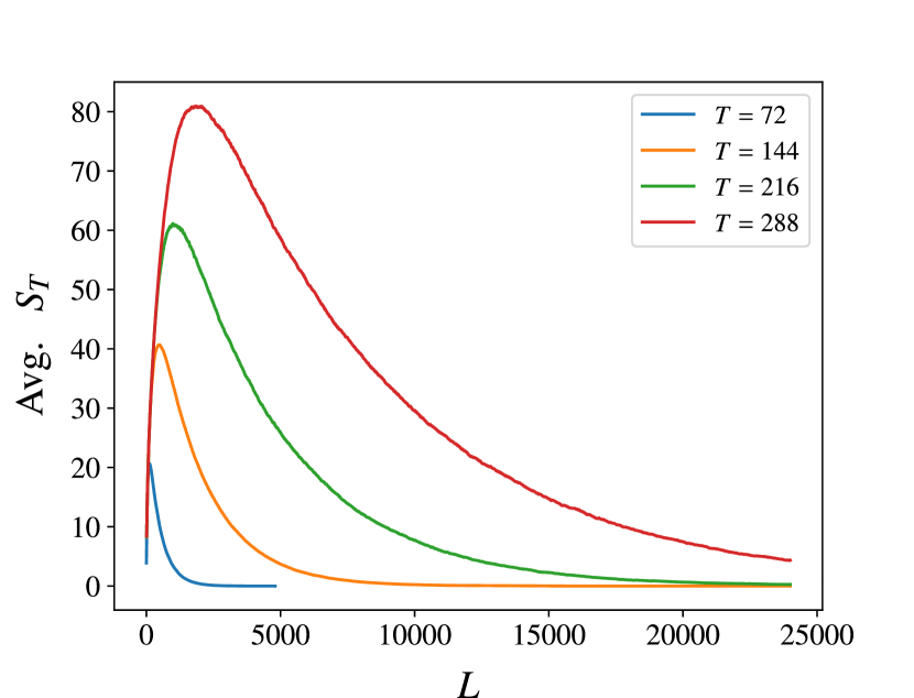
Figure 7: Average temporal entanglement $S_{T}$ plotted against bath size $L$ for measurement rate $p=0.3$ and different total evolution times $T$.

Fig. 7 shows $S_{T}$ as a function of $L$ at $p=0.3$ and for various total evolution times $T$. The peak value of $S_{T}$, $S_{T,\,\text{peak}}$, and the critical bath size at which $S_{T,\,\text{peak}}$ is reached, $L_{c}$, scale as:

$$\begin{split}S_{T,\,\text{peak}}\propto T,\qquad L_{c}\propto T^{2}\,.\end{split}$$ (67)

IV.3 Analytical Understanding of the Initial Growth Regime: Persistent Random Walk

The diffusive growth of temporal entanglement is qualitatively described by a variant of the simple random walk: the persistent random walk [83]. This is analogous to the run-and-tumble model in the context of biophysics and active matter [84]. Consider a random walk model in discrete time on a discrete one-dimensional lattice, where the displacement after $n$ update steps is given by $\sum_{i=1}^{n}\tau_{i}$, where $\tau_{i}=\pm 1$ is the displacement at update step $i$. A movement to the right corresponds to $\tau_{i}=+1$, and a movement to the left corresponds to $\tau_{i}=-1$. The normalized correlation coefficient $\eta$ between successive steps is defined as

$$\eta\equiv\frac{\langle\tau_{i}\tau_{i+1}\rangle}{\langle\tau_{i}^{2}\rangle}=\langle\tau_{i}\tau_{i+1}\rangle\quad\textrm{with}\quad-1<\eta<1,$$ (68)

where $\eta>0$ ($\eta<0$) signifies that successive steps are more likely to be in the same (different) direction, respectively. The limit $\eta=0$ corresponds to the simple random walk, where successive steps are uncorrelated. Away from this limit this model is known as a “persistent random walk”.

The correlation function between two steps separated by $m$ steps in between decays exponentially as $C(m)=\eta^{m}$. The exponentially decaying correlation function implies diffusive behavior after enough update steps, with diffusion constant given by:

$$D(\eta)=\frac{1+\eta}{1-\eta}\,.$$ (69)

If one denotes the probability of switching direction between step $i$ and $i+1$ by $p$, then $\eta=(1-p)-p=1-2p$. In terms of the switching probability, the diffusion constant follows as

$$D(p)=\frac{1-p}{p}\,.$$ (70)

The discussion thereafter uses the all-SWAP circuit as an illustrative example. The argument can be directly extended to explain the same behavior observed in the all-SDKI circuit. In a circuit consisting of SWAP gates, the discussed measurement protocol results in a persistent random walk of the two ends of each Bell pair. The SWAP gates move the Bell-pair ends along the same direction as in the update step before, whereas the identity gate reverses the direction of movement. The measurement rate $p$ thus corresponds exactly to the switching probability $p$, and Eq. (70) can be understood as a relation between the measurement rate and the diffusion constant. Consider, e.g., the following circuit:

(71)

In the first update step no measurement occurs, and both ends of the middle Bell pair propagate in fixed directions. In the second update step a measurement occurs at the right edge of the middle Bell pair, reversing the direction of movement of the right end. Similarly, in the third update step, a measurement occurs at the left edge of the middle Bell pair, reversing the direction of movement of the left end.

The ends of each Bell pair thus undergo a motion of persistent random walk:

$$\begin{split}\langle\Delta t\rangle=\sqrt{2D(p)}\sqrt{\Delta x},\end{split}$$ (72)

where $\langle\Delta t\rangle$ denotes the average temporal displacement of the ends of Bell pairs, and $\Delta x$ denotes an update step in space.

Analogous to the measurement-free setup, we can denote the radius of each Bell pair $r$. With measurements added, the center of mass of each Bell pair is still preserved on average, since the resulted persistent random walk is unbiased. Therefore, $\Delta r$ equals the temporal displacement of one end of the Bell pair: $\Delta r=r^{\prime}-r=\Delta t$. We identify the number of Bell pairs crossing the time point $t_{i}$ as the “local Bell pair density”, denoted $n_{t_{i}}$. Since the Bell pairs are initially uniformly placed, and the update preserves the center of mass on average, the local Bell pair density remains proportional to the average radius of each Bell pair, with a proportionality constant $\kappa$:

$$n_{t_{i}}=\kappa\langle\Delta r\rangle=\kappa\langle\Delta t\rangle,$$ (73)

where $\kappa$ can be interpreted as an effective packing factor.

Since $S_{T}=2\cdot\max_{t_{i}}(n_{t_{i}})$, temporal entanglement is hence expected to grow diffusively with each update step as:

$$\begin{split}S_{T}&=2\cdot\max_{t_{i}}(n_{t_{i}})=2\kappa\langle\Delta t\rangle\\ &=2\kappa\sqrt{2D(p)\Delta x}=2\sqrt{2}\kappa\sqrt{\frac{1-p}{p}}\sqrt{\Delta x}\,.\end{split}$$ (74)

A one-parameter fit is performed on the numerical data with $\kappa$ as the fitting parameter, and the results are shown in Fig. 8. The fitting curve agrees well with numerical data, confirming the proposed functional dependence on $p$, and the optimal fitting value is found as $\kappa\approx 0.36$.

This result shows that the persistent random walk serves well as an effective model describing the growth regime of temporal entanglement with bath size in the presence of measurements.

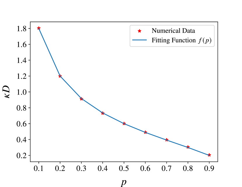
Figure 8: Numerically extracted effective diffusion constant, $\kappa D$, for total evolution time $T=432$. A one-parameter fit using $f(p)=\kappa\sqrt{1-p}/\sqrt{p}$ yields excellent agreement, with $\kappa=0.36$ as the fitting parameter.

IV.4 Analytical Understanding of the Decay Regime: Mixed Spatial Transfer Matrix

Next to the linear growth changing to diffusive growth, the linear decay of the TE with bath size also changes to an exponential decay in the presence of measurements. In order to understand the exponential decay of $S_{T}$ with $L$ and extract the decay scale, we identify a “mixed” spatial transfer matrix, $\mathcal{T}_{p}$, where the averaged TE can be directly calculated by absorbing the measurements into $\mathcal{T}$. This transfer matrix is given by:

$$\begin{split}\mathcal{T}_{p}=\quad\vbox{\hbox{\includegraphics[width=130.08731pt]{mixed_transfer_matrix_2layer.pdf}}}\end{split}$$ (75)

where

$$\begin{split}\vbox{\hbox{\includegraphics[width=65.04034pt]{mixed_gate_2layer1.pdf}}}\equiv(1-p)\cdot\;\vbox{\hbox{\includegraphics[width=65.04034pt]{mixed_gate_2layer2.pdf}}}+p\cdot\vbox{\hbox{\includegraphics[width=65.04034pt]{mixed_gate_2layer3.pdf}}}\end{split}$$ (76)

In order to calculate the averaged TE, numerical tensor contraction is performed to construct $\mathcal{T}_{p}$ with SWAP gates and measurements. Since the spectrum of $\mathcal{T}_{p}$ will determine the exponential decay, the tensor contractions are done without bond-dimension truncation.

That this averaged transfer matrix exactly determines the dynamics of the TE is specific to our setup, and depends on the specific choice of gates and measurements. For extracting the decay scale for purity, one should generally consider constructing the 4-replica $\mathcal{T}_{p}$ rather than the 1-replica $\mathcal{T}_{p}$. However, this is unnecessary for analyzing the SWAP circuit with measurements. Any specific circuit realization will consist out of SWAP gates and identity matrices along the spatial direction, and the action on any initial product state will lead to a “reshuffling” of the initial state, and this reshuffling is independent of the choice of local basis. Furthermore, since the gate choices are locked among replicas, the 4-replica $\mathcal{T}_{p}$ has the same set of eigenvalues as the 1-replica $\mathcal{T}_{p}$, albeit with different degeneracies. This argument directly extends to any calculation of the purity and Rényi entropies (see also Ref. [77]). Within the 1-replica $\mathcal{T}_{p}$, one may further reduce the local Hilbert space dimension from $q=4$ to $q=3$, since the gate choices are also locked between the forward and backward time contours. The detailed construction is presented in Appendix B, and significantly reduces the computational complexity of constructing the transfer matrix, allowing for numerical simulations for longer evolution times.

The leading eigenvalue of $\mathcal{T}_{p}$ satisfy $\lambda_{0}=1$ and corresponds to the perfect-dephaser steady state in the $L\rightarrow\infty$ limit, as can be directly checked. Furthermore, $|\lambda_{i}|<1$ for $i>0$ such that all sub-leading eigenmodes decay exponentially, qualitatively explaining the observed exponential decay of the TE with bath size $L$. These leading eigenvalues of $\mathcal{T}_{p}$ with $T=6$ are plotted against $p$ in Fig. 9. The leading eigenvalues $\lambda_{i}$ with $i=0,1,2,3$ are real and change smoothly with $p$.

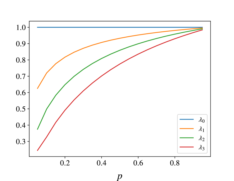
Figure 9: First four leading eigenvalues of the mixed transfer matrix $\mathcal{T}_{p}$ plotted against the measurement rate, $p$, for total evolution time $T=6$.

Fig. 10 compares the decay scale $\xi$ for $S_{T}\propto\exp{(-L/\xi)}$ as extracted from numerical data to the decay scales predicted from $\lambda_{1}$ and $\lambda_{2}$.

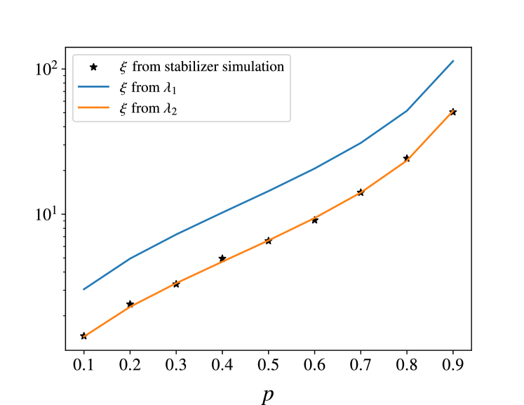
Figure 10: Decay scales for $S_{T}$ as extracted from numerical data and as predicted from $\lambda_{1}$ and $\lambda_{2}$.

In generic cases, one expects the decay scale to be set by the leading nontrivial eigenvalue $\lambda_{1}$, $\xi=-(\log\lambda_{1})^{-1}$. Nevertheless, numerical results indicate that $\xi=-(\log\lambda_{2})^{-1}$. This difference is indicative of a symmetry present in $\mathcal{T}_{p}$.

In order to highlight this symmetry it is convenient to define a local basis for two qubits at the same time point $t_{i}$ on the forward and backward time contours as:

$$\begin{split}|B_{\alpha}\rangle_{i}\;\equiv\quad\vbox{\hbox{\includegraphics[width=69.38078pt]{equal-time_bell.pdf}}}\,,\end{split}$$ (77)

where $\alpha\in\{I,\,X,\,Y,\,Z\}$ again label the four Bell-pair states. Graphically,

$$|B_{I}\rangle\;\equiv\;\vbox{\hbox{\includegraphics[width=13.00806pt]{vacuum_new.pdf}}}\;,\quad|B_{X}\rangle\;\equiv\;\vbox{\hbox{\includegraphics[width=17.34189pt]{xsoliton_new.pdf}}}\;,\quad|B_{Y}\rangle\;\equiv\;\vbox{\hbox{\includegraphics[width=17.34189pt]{ysoliton_new.pdf}}}\;,\quad|B_{Z}\rangle\;\equiv\;\vbox{\hbox{\includegraphics[width=17.34189pt]{zsoliton_new.pdf}}}\,.$$ (78)

The trace projector at the temporal boundary $t=T$ projects onto the $|B_{I}\rangle$ mode and annihilates the X, Y, and Z states. The product state of $|B_{I}\rangle$ modes $|\circ\circ\dots\circ\circ\rangle$ corresponds to the perfect dephaser state and is an eigenstate of $\mathcal{T}_{p}$. We can denote the $|B_{I}\rangle$ mode as a reference state and the $|B_{X}\rangle$, $|B_{Y}\rangle$, $|B_{Z}\rangle$ modes as X-, Y- and Z-particles.

Consider the SWAP circuit with measurements. One trajectory realization may then, for example, look like the following:

(79)

The actions of the SWAP and the identity gates both preserve the number and flavors of the particles (i.e. whether these are X, Y or Z Bell pairs), and the particles merely get shuffled around. The only operator that does not conserve the particle number is the projector, which however annihilates the state if it acts on a particle, such that $\mathcal{T}_{p}$ does not couple sectors with different number and flavors of particles. Consequently, $\mathcal{T}_{p}$ decomposes into symmetry sectors corresponding to fixed numbers of particles:

$$\mathcal{T}_{p}=\mathcal{T}^{(0)}_{p}\otimes\mathcal{T}^{(1)}_{p}\otimes\ldots\otimes\mathcal{T}^{(T-1)}_{p}\,,$$ (80)

where the superscript denotes the number of particles in the sector.

For simplicity, we assume that all particles are of the same flavor; predictions obtained under such simplification already match the numerical results. The first few leading eigenvalues, which are all real, correspond to the leading eigenvalues of the lowest particle-number sectors, i.e. $\lambda_{0}\leftrightarrow\mathcal{T}_{p}^{(0)}$, $\lambda_{1}\leftrightarrow\mathcal{T}_{p}^{(1)}$, $\lambda_{2}\leftrightarrow\mathcal{T}_{p}^{(2)}$, etc. In order to have a finite entanglement in the system, one needs at least one Bell pair connecting some $t_{i}$ to some $t_{j}$ on the same time contour. Such a Bell pair however requires at least two particles in the system. E.g., two replicas of a Bell pair connecting different times in two time contours can be expressed as a linear combination of four Bell pairs connecting the same times between different time contours:

$$\begin{split}\vbox{\hbox{\includegraphics[width=86.72267pt]{adjacent_bell.pdf}}}\quad=\quad\frac{1}{2}(&|B_{I}\rangle_{i}|B_{I}\rangle_{i+1}+|B_{X}\rangle_{i}|B_{X}\rangle_{i+1}\\ &+|B_{Y}\rangle_{i}|B_{Y}\rangle_{i+1}+|B_{Z}\rangle_{i}|B_{Z}\rangle_{i+1}).\end{split}$$ (81)

Therefore, neither the zero-particle perfect dephaser sector nor the one-particle sector contribute to the overall temporal entanglement of the system. The two-particle sector, $\mathcal{T}_{2}$, is the leading sector that contributes to the total temporal entanglement. Moreover, $\mathcal{T}_{2}$ can contribute an extensive amount of entanglement in the form of superposition of states. The eigenvalue that sets the decay scale for $S_{T}$ is therefore $\lambda_{2}$. Since $\lambda_{2}$ changes smoothly with $p$, the decaying part of $S_{T}$ also changes smoothly with $p$.

It is now worth comparing the structure of $\mathcal{T}_{p}$ with measurements to the structure of $\mathcal{T}$ in the measurement-free case. $\mathcal{T}$ for the purely unitary circuit consists of a $1\times 1$ block $\mathcal{T}^{(0)}$ corresponding to the steady state with eigenvalue $\lambda_{0}=1$ and Jordan blocks of various sizes,

$$\mathcal{T}=\mathcal{T}^{(0)}\otimes Q_{2}\otimes Q_{3}\otimes\ldots\otimes Q_{T-1}\,.$$ (82)

Each Jordan block $Q_{i}$ has its corresponding eigenvalue zero since these are necessarily nilpotent. This is necessary to exactly reach the perfect dephaser limit after a finite number of update steps. The largest Jordan block $Q_{T-1}$ is of size $(T-1)\times(T-1)$, which vanishes after being raised to the $T$-th power, $(Q_{T-1})^{T}=0$, such that temporal entanglement decays linearly with bath size rather than exponentially and an exact steady state is reached at bath size $L=T$.

This structure is in stark contrast to the structure of $\mathcal{T}_{p}$ for circuits with measurements. In $\mathcal{T}_{p}$, the Jordan blocks are no longer nilpotent. Instead of having all eigenvalues being zero, the Jordan blocks now have nontrivial diagonal elements. As such, the decay of temporal entanglement is again exponential in bath size. Any infinitesimal measurement rate immediately induces this structural change in the transfer matrix, since the appearance of nilpotent Jordan blocks generally requires fine-tuning.

IV.5 Peak Value of Temporal Entanglement and the Critical Bath Size

In between the growth and decay regimes, the TE reaches a peak value that will set the temporal entanglement barrier. The critical bath size $L_{c}$ is the bath size at which the peak value of $S_{T}$ is attained, and we observe numerically that

$$L_{c}(T,p)\propto\frac{T^{2}}{D(p)},$$ (83)

as shown in Figs. 11 and 12.

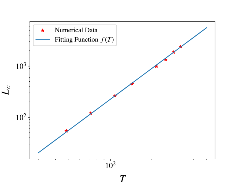
Figure 11: Scaling of $L_{c}$ with $T$. The data is fitted with a one-parameter function of the form $f(T)\propto T^{2}$.

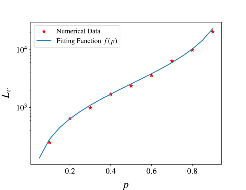
Figure 12: Scaling of $L_{c}$ with $p$. The data is fitted with a one-parameter function of the form $f(p)\propto p/(1-p)$.

In both circuits with and without measurements, $L_{c}$ is reached when all the temporal Bell pairs initially in the interval $2T/3\leq t<T$ have their left ends hitting the temporal boundary. This condition can be understood in the measurement-free setup as follows: for $L<L_{c}$, entanglement builds up in the interval $0<t<2T/3$ and decays in the interval $2T/3<t<T$. At $L=L_{c}$, entanglement in the interval $0<t<2T/3$ is “saturated”, with all $T/3$ Bell pairs forming a rainbow state:

$$\begin{split}|\Psi_{\text{RB}}\rangle=\quad&\vbox{\hbox{\includegraphics[width=260.17464pt]{rainbow_state_new.pdf}}}\end{split}$$ (84)

The optimal bipartition is at $t_{i}=T/3$, and the peak entanglement is given by the number of Bell pairs crossing the bipartition on both the forward and backward time contours: $S_{T,\,\text{peak}}=2\cdot T/3=2T/3$. For $L>L_{c}$, ends of Bell pairs start reflecting at $t=0$, and the rainbow state is destroyed. The maximal entanglement thus starts decreasing.

With measurements, the ends of Bell pairs spread diffusively:

$$\begin{split}\sqrt{2DL_{c}}=\Delta t=\frac{T}{3}\quad\Rightarrow L_{c}=\frac{(\Delta t)^{2}}{2D}=\frac{T^{2}}{18D},\end{split}$$ (85)

which matches the numerically observed scaling of Eq. (83). At $L=L_{c}$, entanglement in the interval $0<t<2T/3$ is saturated on average, with the only difference with the case without measurements being that the Bell pairs in this interval no longer form a rainbow state. Upon adding random measurements and resulting random distributions of Bell pairs, for different distribution the TE ranges from a minimal value of zero to a maximal value given by that of the rainbow state. The averaged value the reaches a steady state of exactly half the maximum value, independent of $p$, resulting in a peak value $S_{T,\,\text{peak}}$ with measurements that is half that without measurements.

V Non-Hermitian Phase Transition in the Mixed Transfer Matrix Spectrum

While the exponential decay of the TE for large bath sizes is fully set by the leading eigenvalue of the transfer matrix, the intermediate dynamics generally requires knowledge of the full eigenspectrum. The leading eigenvalue was already observed to be real, resulting in purely exponential decay, but in general it is not guaranteed that the eigenvalues of the transfer matrix are real. In this Section we will show that both the eigenspectrum and the eigenstates of the transfer matrix – except for the leading eigenvalue – change qualitatively as the measurement rate is varied, indicating nonanalytic transitions in the “dynamics” of the averaged TE as the measurement rate is varied.

The spatial transfer matrix is non-Hermitian and hence not guaranteed to be diagonalizable or have real eigenvalues. The eigenspectrum is however constrained because the transfer matrix generally possesses PT (parity-time) symmetry: it is invariant under the combined action of a unitary parity operator, here the exchange of the forward and backward time contour, and an anti-unitary time reversal operator, here complex conjugation. While this symmetry is readily apparent for our choice of gates, resulting in purely real transfer matrices that are invariant under complex conjugation, this symmetry holds more generally.

Eigenvalues of PT-symmetric matrices are constrained to be either real of part of a complex conjugate pair. As pointed out in Refs. [85, 86], certain non-Hermitian matrices with PT symmetry possess spectra that are entirely real, in which case the system is said to be in a PT-symmetric phase. The spectrum of PT-symmetric Hamiltonian can change nonanalytically as some underlying parameter is tuned, and the PT-symmetry can be spontaneously broken when the spectrum changes from purely real to being a combination of complex-conjugate pairs of eigenvalues and real eigenvalues [85]. The PT-broken phase is known to host a proliferation of exceptional points (EPs) at which the model is not diagonalizable but rather exhibits Jordan blocks [87, 88, 89].

For the spatial transfer matrix (14) such a transition is observed at a critical measurement rate $p_{c}=1/2$. For $1/2<p<1$ all eigenvalues are purely real, whereas for $0<p<1/2$ the PT symmetry is spontaneously broken in all sectors $\mathcal{T}_{p}^{(i)}$ with $i>1$ and the spectrum contains pairs of complex conjugate eigenvalues. This is illustrated in Fig. 13, showing the spectra of the two-particle sector, $\mathcal{T}_{p}^{(2)}$, for total evolution time $T=6$.

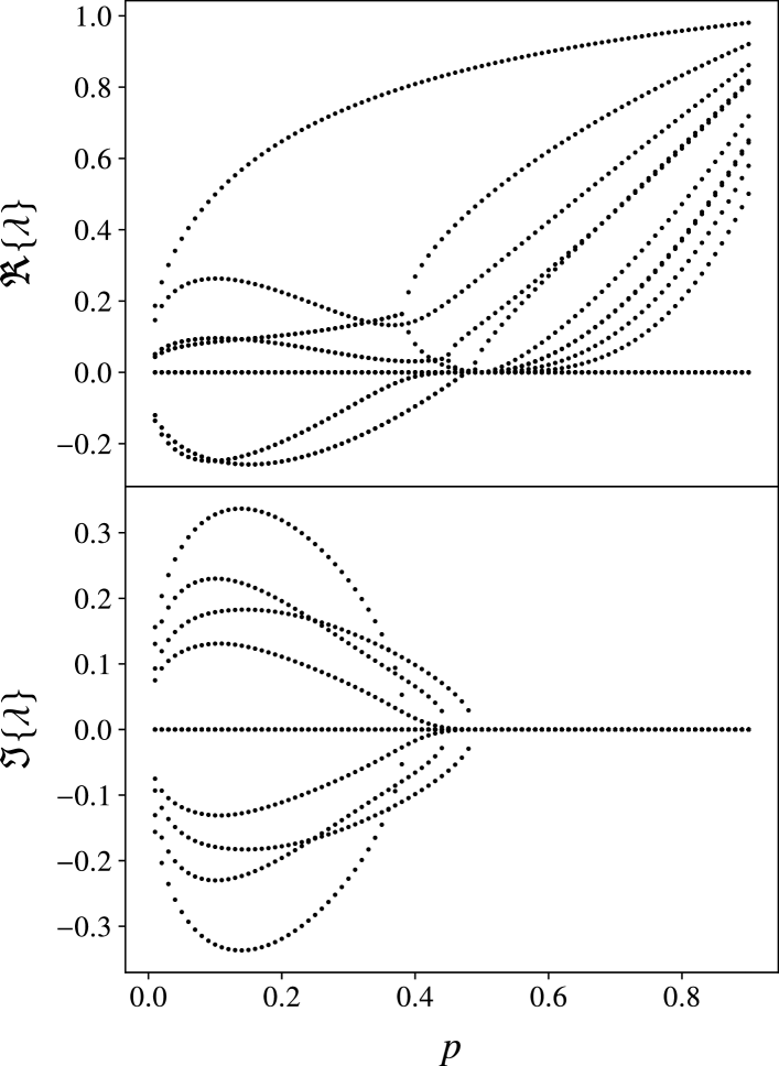
Figure 13: Real and imaginary parts of the spectra of $\mathcal{T}_{p}^{(2)}$ for total evolution time $T=6$ and varying measurement rates $p$.

In order to understand the critical measurement rate $p_{c}=1/2$, it is instructive to rewrite the transfer matrix as a non-Hermitian Hamiltonian. We consider the simplest example of the one-particle sector, which has a natural choice of basis, e.g. for $T=6$:

$$\begin{split}|1\rangle&\equiv|\bullet\circ\circ\circ\circ\circ\rangle\\ |2\rangle&\equiv|\circ\bullet\circ\circ\circ\circ\rangle\\ |3\rangle&\equiv|\circ\circ\bullet\circ\circ\circ\rangle\\ |4\rangle&\equiv|\circ\circ\circ\bullet\circ\circ\rangle\\ |5\rangle&\equiv|\circ\circ\circ\circ\bullet\circ\rangle\\ |6\rangle&\equiv|\circ\circ\circ\circ\circ\bullet\rangle\end{split}$$ (86)

Here $\ket{\circ}$ and $\ket{\bullet}$ correspond to the particle notation of Eq. (78). The matrix elements of the spatial transfer matrix can be analytically obtained in closed form, resulting in a hopping Hamiltonian with symmetric nearest-neighbor hopping and uni-directional next-nearest neighbor hopping, with the hopping direction being different depending on whether the lattice site is odd or even. For a single particle the transfer matrix $\mathcal{T}_{p}^{(1)}$ can be written as a non-Hermitian Hamiltonian:

$$H= \,p^{2}\sum_{j=2}^{T-1}|j\rangle\langle j|+J_{1}\sum_{j=2}^{T-2}\left(|j\rangle\langle j-1|+|j\rangle\langle j+1|\right)$$

$$+J_{2}\sum_{\begin{subarray}{c}j=2\\ j\,\textrm{even}\end{subarray}}^{T-2}|j\rangle\langle j+2|+J_{2}\sum_{\begin{subarray}{c}j=3\\ j\,\textrm{odd}\end{subarray}}^{T-3}|j\rangle\langle j-2|$$

$$+p|1\rangle\langle 1|+(1-p)|1\rangle\langle 2|\,,$$ (87)

with nearest-neighbor hopping amplitude $J_{1}=p(1-p)$ and next-nearest-neighbor hopping amplitude $J_{2}=(1-p)^{2}$. This model is illustrated in Fig. 14, where the lattice is divided into odd and even sub-lattices. Both the boundary terms and the next-to-nearest-neighbor interaction are explicitly non-Hermitian. In higher-particle sectors the corresponding Hamiltonian has the same hopping amplitudes, as well as an additional hard-core constraint on the particles.

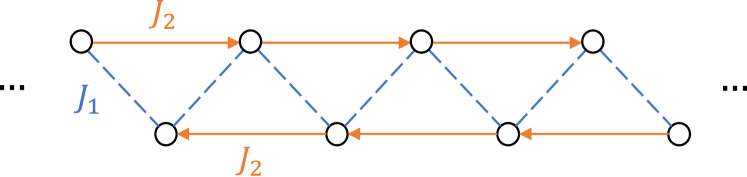
Figure 14: Hopping model for the spatial transfer matrix restricted to a single particle. The lattice is divided into odd and even sub-lattices to account for the even-odd dependence in hopping amplitudes. $J_{1}$ is the symmetric nearest-neighbor hopping amplitude; $J_{2}$ is the uni-directional next-nearest-neighbor hopping amplitude.

This model can be explicitly solved in the one-particle sector, with the solution being representative of the physics in the higher-particle sector. It is instructive to first consider the model with periodic boundary conditions, i.e.

$$H_{\textrm{PBC}}= \,p^{2}\sum_{j=1}^{T}|j\rangle\langle j|+J_{1}\sum_{j=1}^{T}\left(|j\rangle\langle j-1|+|j\rangle\langle j+1|\right)$$

$$+J_{2}\sum_{j\,\textrm{even}}|j\rangle\langle j+2|+J_{2}\sum_{j\,\textrm{odd}}|j\rangle\langle j-2|,$$ (88)

where we identify $j+T=j$. The periodic boundary conditions allow this model to be solved by going to Fourier space, writing an eigenstate $\ket{\psi}$ with components

$$\psi_{j}=\begin{cases}\alpha_{+}e^{ikj}+\alpha_{-}e^{-ikj},\qquad&\textrm{for}\,j\,\textrm{even},\\ \beta_{+}e^{ikj}+\beta_{-}e^{-ikj},\qquad&\textrm{for}\,j\,\textrm{odd}.\end{cases}$$ (89)

The coefficients $\alpha_{\pm}$ and $\beta_{\pm}$ can be obtained by solving the eigenvalue equation in Fourier space:

$$\begin{bmatrix}p^{2}+J_{2}e^{-2ik}&2J_{1}\cos{k}\\ 2J_{1}\cos{k}&p^{2}+J_{2}e^{2ik}\end{bmatrix}\begin{bmatrix}\alpha_{\pm}\\ \beta_{\pm}\end{bmatrix}=\lambda\begin{bmatrix}\alpha_{\pm}\\ \beta_{\pm}\end{bmatrix},$$ (90)

which additionally returns the dispersion relation, giving a pair of eigenvalues $\lambda_{\pm}$ as a function of the momentum $k$:

$$\lambda_{\pm}(k)=1-2J_{1}-2J_{2}\sin^{2}k\pm 2\cos{k}\sqrt{J_{1}^{2}-J_{2}^{2}\sin^{2}k}\,.$$ (91)

The periodic boundary conditions quantize $k=2\pi n/T,n=0,1\dots T-1$.

The non-Hermitian Hamiltonian with periodic boundary conditions already highlights how the structure of the eigenspectrum is determined by the relative magnitudes of the (positive) hopping amplitudes $J_{1}$ and $J_{2}$. In the regime $J_{1}>J_{2}$ and hence $p>1/2$, all eigenvalues (91) are purely real for all $k$-modes. For $J_{1}<J_{2}$, a transition from complex to real eigenvalues occurs for the $k$-mode satisfying $\sin{k}=J_{1}/J_{2}=p/(1-p)$. The first complex eigenvalues are possible at $J_{1}=J_{2}$ and hence $p=1/2$, with a proliferation of exceptional points occurring in the $J_{1}<J_{2}$ regime corresponding to $0<p<1/2$. In the former regime the Hermitian nearest-neighbor hopping is the dominant contribution in the Hamiltonian and the eigenvalues are purely real, whereas in the latter regime the unidirectional hopping dominates the dynamics and results in strongly non-Hermitian dynamics. However, while the eigenvalues exhibit a qualitative change as $p$ is varied, the eigenstates remain plane waves at any measurement rate.

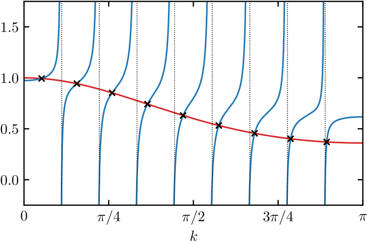
Figure 15: Graphical illustration of both sides of the quantization condition [Eq. (92)] for the momentum with $\lambda(k)=\lambda_{+}(k)$ for total evolution time $T=10$ and measurement rate $p=0.8$. Vertical dotted lines indicate the approximate poles $k=n\pi/(T-1),n=1\dots T-2$, and crosses indicate the solutions for the quantized momentum $k$ at the intersections between the left-hand side (red) and right-hand side (blue line).

Taking into account the exact boundary conditions from Eq. (V), the ansatz (89) still returns the exact eigenstates, but the momentum $k$ now needs to be determined in a self-consistent way. As shown in Appendix E, for the boundary conditions in the spatial transfer matrix the eigenvalue $\lambda(k)$ needs to satisfy

$$\lambda(k)=p\frac{\lambda(k)-p^{2}+J_{2}}{\lambda(k)-p^{2}-J_{2}\sin(k(T-3))/\sin(k(T-1))},$$ (92)

where $\lambda(k)=\lambda_{\pm}(k)$ [both choices of the sign lead to the same solutions since $\lambda_{+}(k)=\lambda_{-}(\pi-k)$]. This equation is graphically illustrated in Fig. 15 in the regime where $p>1/2$ and all eigenvalues are real.

The left-hand side is a smooth function of $k$, whereas the right-hand side exhibits a series of vertical asymptotes in between which this function is monotonically increasing for $0<k<\pi$. The corresponding poles are located at the values of $k$ for which

$$\frac{\lambda(k)-p^{2}}{J_{2}}=\frac{\sin(k(T-3))}{\sin(k(T-1))}.$$ (93)

The locations of these poles can be approximately determined when $p\approx 1$. In this limit we have that $(\lambda(k)-p^{2})/J_{2}\gg 1,\forall k,$ such that the poles need to satisfy $\sin(k(T-1))\approx 0$, leading to poles at the quantized momentum values $k=n\pi/(T-1),n=1\dots T-2$. In between any pair of neighboring poles a solution to the self-consistent equation can be found, returning the expected $T-1$ nontrivial eigenvalues, with $\lambda=0$ the remaining trivial eigenvalue. The number of poles remains fixed for $p>1/2$ and in this way all eigenstates in the regime $p>1/2$ can be obtained. We find that in this regime all eigenvalues are real and the eigenstates resemble the plane waves also observed for periodic boundary conditions.

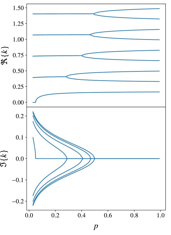
Figure 16: Quantized values of the momentum $k$ solving the quantization condition [Eq. (92)] for total evolution time $T=10$ as function of the measurement rate $p$. For $p>1/2$ all momenta and the corresponding eigenvalues are real, whereas for $p<1/2$ a series of exceptional points occur at which two real momenta and corresponding eigenvalues coalesce and continue as a pair of complex conjugate eigenvalues. At $p=1/(2T)$ the value of $k$ associated with the leading eigenvalue changes from purely real to purely imaginary.

For $p<1/2$ all eigenvalues can still be found as solutions to the self-consistent equation (92), but now both the eigenvalue and the corresponding momentum can be complex. The poles move into the complex plane as $p$ is decreased, requiring complex values of $k$ in order to satisfy Eq. (92). In Fig. 16 we show the resulting values of the momentum as function of $p$ for a small system size of $T=10$. As opposed to the case with periodic boundary conditions, the corresponding eigenstates are no longer given by plane waves but rather by states localized at the (temporal) boundaries. Any nonzero imaginary part in $k$ results in an exponential decay in the eigenstates away from the boundaries $t=0$ and $t=T$, inducing localization at the boundaries reminiscent of the non-Hermitian skin effect [73, 90, 91].

However, as can also be observed in Fig. 9, the leading eigenvalue is always real. The corresponding momentum $k$ changes from purely real to purely imaginary at $p=1/(2T)$, at which point the eigenstates again decay exponentially away from the temporal boundaries – with a localization length that is however on the order of $T$, such that the wave function is still supported on the full system of $T$ sites. Exactly at $p=1/(2T)$ the eigenstates have a linear profile (see Appendix E). That the leading eigenvalue is real can be understood from the PT-symmetry: for an even number of eigenvalues it is not possible for all eigenvalues to be part of a complex conjugate pair since $\lambda=0$ is always a real eigenvalue, requiring an additional real eigenvalue in the spectrum.

This argument directly extends to the 2-particle sector governing the decay of temporal entanglement. While the above derivation focused on the single-particle sector, results in the two-particle sector are qualitatively similar, indicating that for large $T$ the interaction between the two particles can be treated perturbatively. The non-Hermitian transition is observed in the spectra of $\mathcal{T}_{p}$, but the decay behavior of temporal entanglement with bath size does not show any non-analyticity with $p$. The leading eigenvalue in the 2-particle sector is both real and smooth for all values of $p$. As such, the transition in the eigenspectrum at $p=1/2$ will only be observable in any transient behavior.

VI Generality of the Results: SDKI circuits and the Dual-Unitary Clifford Class

All presented results with and without measurements can be numerically checked to agree exactly for both the SWAP and SDKI circuits. This section explains why the simple diffusion picture based on SWAP circuits with measurements holds also for SDKI circuits using insights from the stabilizer formalism [63]. In the stabilizer formalism, a quantum state is represented by the set of operators that stabilize it. Given a state $|\psi\rangle$, the stabilizer set is defined as

$$\mathcal{S}=\{S\,|\,S|\psi\rangle=|\psi\rangle\},$$ (94)

and instead of evolving the state, one evolves the stabilizer set as

$$\begin{split}\mathcal{S}\rightarrow U\mathcal{S}U^{\dagger},\end{split}$$ (95)

where for each $S_{i}\in\mathcal{S}$, $S_{i}\rightarrow US_{i}U^{\dagger}$. The action of an operator $U$ on a stabilizer string $S_{i}$ is denoted as $U(S_{i})=US_{i}U^{\dagger}$.

For $n$ sites, the basis consists of Pauli strings of the form $P^{(n)}=P_{1}\otimes P_{2}\otimes\ldots\otimes P_{n}$, where the single-site Pauli operator is $P_{i}\in\{I,X,Y,Z\}$. By construction, stabilizer circuits map one Pauli string to another Pauli string without generating superposition of Pauli strings. One may separate a Pauli string into an X-string and a Z-string and keep track of the stabilizer action on each string separately. Therefore, for a 2-site gate $U^{(2)}$, its action on $\{IX,XI,IZ,ZI\}$ completely defines its action on all $P^{(2)}$.

The actions of the SWAP and the SDKI gates are as follows:

$$\begin{split}\text{SWAP}(ZI)&=IZ,\quad\quad\text{SDKI}(ZI)=XZ,\\ \text{SWAP}(IZ)&=ZI,\quad\quad\text{SDKI}(IZ)=ZX,\\ \text{SWAP}(XI)&=IX,\quad\quad\text{SDKI}(XI)=IX,\\ \text{SWAP}(IX)&=XI,\quad\quad\text{SDKI}(IX)=XI.\end{split}$$ (96)

The SWAP gate simply moves the $Z$ and $X$ operators around. The SDKI acts in the same way on the $X$ operators, but has a more complicated action on the $Z$ operator: whenever a $Z$ operators hops away from a lattice site, it “emits” an $X$ operator backward such that there is now an additional $X$ operator on the original site.

The stabilizer set for a Bell pair connecting sites $t_{i}$ and $t_{i+1}$,

$$|\phi\rangle_{i,\,i+1}=\;\vbox{\hbox{\includegraphics[width=78.04842pt]{bell_pair_labeled.pdf}}},$$ (97)

is given by

$$\mathcal{S}\left(|\phi\rangle\right)=\{\, I_{1}I_{2}\ldots I_{i-1}X_{i}X_{i+1}I_{i+2}\ldots I_{T},\;$$

$$I_{1}I_{2}\ldots I_{i-1}Z_{i}Z_{i+1}I_{i+2}\ldots I_{T}\,\}\,.$$ (98)

Starting from the state $|\Phi\rangle=\bigotimes|\phi\rangle$, under the action of the SWAP gates the $IXXI$ and $IZZI$ stabilizers spread into $XIIX$ and $ZIIZ$, respectively:

$$\begin{split}(\text{SWAP}\otimes\text{SWAP})(IXXI)&=XIIX,\\ (\text{SWAP}\otimes\text{SWAP})(IZZI)&=ZIIZ.\end{split}$$ (99)

For the SDKI circuit the $IXXI$ and $IZZI$ stabilizers spread as

$$\begin{split}(\text{SDKI}\otimes\text{SDKI})(IXXI)&=XIIX,\\ (\text{SDKI}\otimes\text{SDKI})(IZZI)&=ZXXZ.\end{split}$$ (100)

The end points of both operator strings spread in the same way in both circuits. For the operator strings with $X$ operators as endpoints, the operators in between are given by the identity, whereas for the operator strings with $Z$ operators as endpoints the operators in between are either the identity for the SWAP circuit or $X$ operators for the SDKI circuit. This result holds more generally: the end points of the stabilizers in both circuits undergo identical evolution, with and without measurements, with the only difference being that for operators whose endpoints are $Z$ these are either of the form $ZII\dots IIZ$ for the SWAP circuit or $ZXX\dots XXZ$ for the SDKI circuit. Acting on the bulk of the operator strings, i.e. not the endpoints, leaves the internal structure invariant since both gates leave $II$ and $XX$ invariant. Acting on the endpoints with the gates either grows or shrinks the length of the string, but again leaves the structure in between invariant. Consider e.g. the right endpoints, for which the relevant actions are

$$\text{SWAP}(ZI)=IZ, \quad\text{SWAP}(IZ)=ZI,$$ (101)

$$\text{SDKI}(ZI)=XZ, \quad\text{SDKI}(XZ)=ZI,$$ (102)

and similar for the left end points

$$\text{SWAP}(IZ)=ZI, \quad\text{SWAP}(ZI)=IZ,$$ (103)

$$\text{SDKI}(IZ)=ZX, \quad\text{SDKI}(ZX)=IZ.$$ (104)

This argument directly extends to the case with measurements, since we have already argued that the entanglement structure can be obtained from the case with forced measurements on a single Bell state whose space-time dual is the identity, and acting with the identity again leaves the structure of the operator strings intact. Crucially, the endpoints of the operator strings completely determine the entanglement structure of the state [17]. As such, the precise Pauli operators in the bulk of the string are irrelevant, and both SWAP and SDKI circuits produce the same entanglement dynamics.

VII Conclusion

In this work, we characterized the shape of the temporal entanglement barrier in dual-unitary Clifford circuits with and without measurements. By leveraging the spatial unitarity of the circuit, we are able to efficiently simulate the evolution of the influence matrix with bath size and obtain the temporal entanglement profile in both space and time.

In circuits without measurements, the observed linear growth and decay of TE are explained through exact tensor network contractions. In the presence of measurements, the linear growth underlied by ballistic spreading of temporal Bell pairs is modified to a diffusive growth. The functional dependence of the diffusion constant on the measurement rate is explained by considering the persistent random walk motion of the ends of the temporal Bell pairs. This diffusion picture for temporal Bell pairs can also be used to predict the peak value of TE and the critical bath size at which this peak is reached.

Rather than exactly reaching the perfect dephaser limit with vanishing TE at a finite bath size, the decay of the TE to this limit becomes exponential in the presence of measurements. The corresponding characteristic decay scales are explained by constructing a mixed spatial transfer matrix, identifying a symmetry, and examining its eigenspectrum in different symmetry sectors. By tuning the measurement rate, the decay rate can be made arbitrarily slow, vanishing in the limit of purely measurement dynamics.

The temporal entanglement barrier always scales linearly with the number of time steps, similar to volume law entanglement, such that there is no measurement-induced phase transition in the current setup. However, although no nonanalyticity shows up in the TE as the measurement rate is tuned, there is a PT phase transition in the eigenspectrum of the mixed spatial transfer matrix at $p=1/2$. This transition can be understood in a specific symmetry sector, where we find that both the eigenvalues and eigenstates exhibit a quantitative change, with the latter localizing at the temporal boundaries. It would be interesting to explore conditions for which the PT transitions manifest itself in the dynamics of TE, for instance by restricting to particular sets boundary states. Going beyond the current work, it would be worth investigating the interplay between measurements and temporal entanglement in more generic setups. The mapping of the spatial dynamics to a non-Hermitian hopping model furthermore suggests using space-time duality as a way of realizing non-Hermitian dynamics.

Appendix A Temporal Entanglement Profile of Generic Dual-Unitary Clifford Circuits without Measurements

This section presents numerical results on the temporal entanglement profile for dual-unitary Clifford circuits where Eq. (53) does not hold. This situation can occur either because the gates fail to be both self-dual and real or because the circuit fails to be translationally invariant in space and time, or a combination of both. In this case the diagrams (50) and (55) cannot be analytically evaluated. We will first consider circuits of random dual-unitary Clifford circuits that are inhomogeneous in both time and space, before consider homogeneous circuits that do not satisfy Eq. (53).

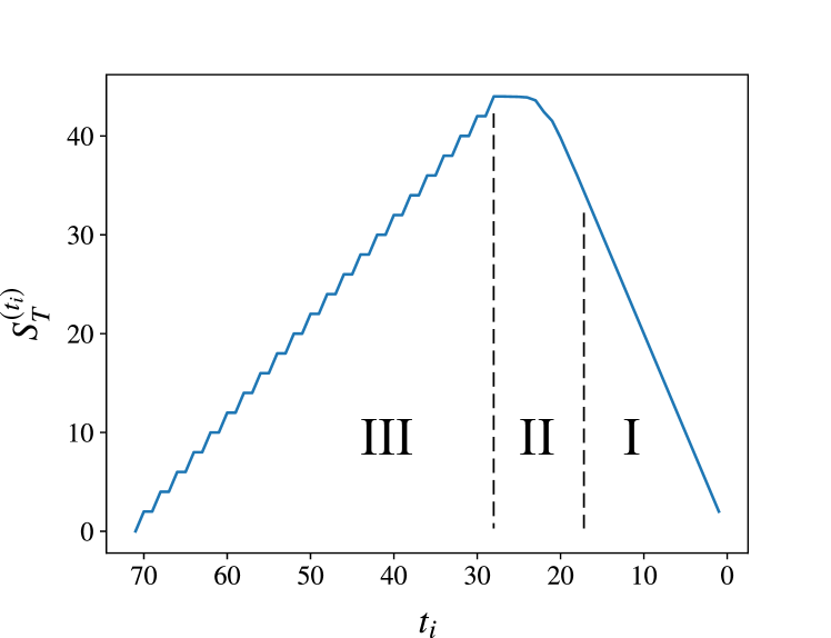
Figure 17: Temporal entanglement plotted against temporal bipartition point $t_{i}$, with total evolution time $T=72$ and bath size $L=28$. The circuit consists of random dual-unitary Clifford gates, and the results are averaged over $N=100$ realizations. There are 3 bipartition intervals, each showing different phenomenologies. Interval I is $0<t_{i}<T-2L$, Interval II is $T-2L\leq t_{i}<L$, and Interval III is $L\leq t_{i}<T$.

Fig. 17 shows $S_{T}^{(t_{i})}$ as function of $t_{i}$ for $T=72$ and $L=28$ with random dual-unitary Clifford gates. The parameter choice corresponds to Regime 2.

While qualitatively similar to Fig. 4, there is a quantitative difference: Instead of nonanalytically changing the slope to half of that in Interval I, $S_{T}^{(t_{i})}$ maintains the same slope as in Interval I upon entering Interval II, before flattening out.

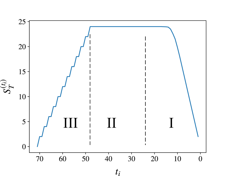
Figure 18: Temporal entanglement plotted against temporal bipartition point $t_{i}$, with total evolution time $T=72$ and bath size $L=48$. The circuit consists of random dual-unitary Clifford gates, and the results are averaged over $N=100$ trajectories. There are 3 bipartition intervals, each showing different phenomenologies. Interval I is $0<t_{i}<2L-T$, Interval II is $2L-T\leq t_{i}<L$, and Interval III is $L\leq t_{i}<T$.

Fig. 18 shows $S_{T}^{(t_{i})}$ as function of $t_{i}$ for $T=72$, $L=48$ with random dual-unitary Clifford gates. The parameter choice corresponds to Regime 3. The contracted diagram correspond to Eq. (55) in Interval I and Eq. (50) in Interval II, respectively. Contrasting with Fig. 5, $S_{T}^{(t_{i})}$ behaves differently in these intervals: In Interval I, instead of having always $S_{T}^{(t_{i})}=0$, $S_{T}^{(t_{i})}$ grows linearly with $t_{i}$ and saturates to the peak value somewhere in the middle of Interval I. In Interval II, $S_{T}^{(t_{i})}$ remains constant at the peak value instead of growing linearly with $t_{i}$.

We next consider the following gate obtained by applying Hadamard gates to the left input and out legs of the Clifford SDKI gate:

$$(H\otimes I)\,\text{SDKI}\,(H\otimes I)$$ (105)

This gate does not satisfy the condition given in Eq. (53). Fig. 19 shows the resulting $S_{T}^{(t_{i})}$ as function of $t_{i}$ for $T=72$, $L=28$. The parameter choice corresponds to Regime 2. In Interval II, the contracted diagram is of the form (50). Contrasting with Fig. 4, the temporal entanglement now behaves similarly as in the case of inhomogeneous dual-unitary Clifford gates.

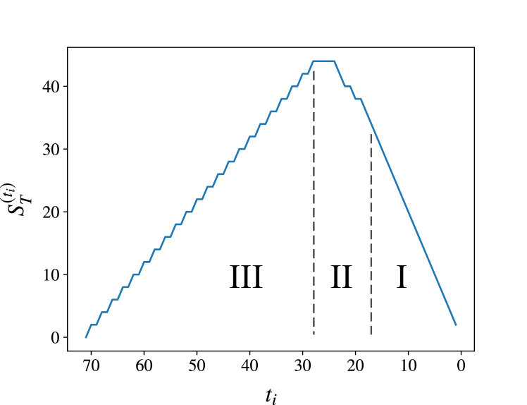
Figure 19: Temporal entanglement plotted against temporal bipartition point $t_{i}$, with total evolution time $T=72$ and bath size $L=28$. The circuit consists of only gates of the form (105). There are 3 bipartition intervals, each showing different phenomenologies. Interval I is $0<t_{i}<T-2L$, Interval II is $T-2L\leq t_{i}<L$, and Interval III is $L\leq t_{i}<T$.

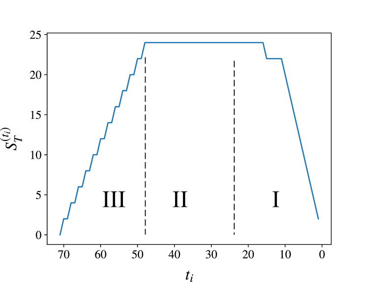
Figure 20: Temporal entanglement plotted against temporal bipartition point $t_{i}$, with total evolution time $T=72$ and bath size $L=48$. The circuit consists of only $\text{SDKI}^{\text{(lH)}}$ gates. There are 3 bipartition intervals, each showing different phenomenologies. Interval I is $0<t_{i}<2L-T$, Interval II is $2L-T\leq t_{i}<L$, and Interval III is $L\leq t_{i}<T$.

Fig. 20 shows $S_{T}^{(t_{i})}$ as function of $t_{i}$ for $T=72$, $L=48$ with gates of the form (105) in Regime III. The contracted diagram is of the form Eq. (55) and Eq. (50) in Interval I and II, respectively. We again observe the same behavior as for inhomogeneous dual-unitary Clifford gates.

Overall, failure to fulfill Eq. (53) leads to a drastic change in the behavior of $S_{T}^{(t_{i})}$ in intervals where the simplified diagram is form Eq. (50) or Eq. (55).

Nonetheless, the maximal value and the corresponding TE remains the same regardless of whether Eq. (53) is fulfilled or not. Therefore, the temporal entanglement profile given by Eq. (31) remains valid for all dual-unitary Clifford circuits and is insensitive to the condition of Eq. (53).

Appendix B Numerically Exact Results on Temporal Entanglement with Measurements: Tensor Contraction of the Mixed Transfer Matrix

This section details the procedure for computing $S_{T}$ through tensor contraction of $\mathcal{T}_{p}$. The procedure does not involve averaging over stochastic trajectories and thus avoids stochastic noise. It is convenient to temporarily fix the normalization factor $\operatorname{tr}\left((\rho^{\langle I_{\text{left}}|})^{2}\right)=1$. Although the purity $D_{t_{i}}^{\langle\text{left}|}$ is nonlinear in $\left|\rho^{\langle\text{left}|}\right\rangle$, it is linear in $\left|\rho^{\langle\text{left}|}\right\rangle^{\otimes 4}$. Graphically, one may define:

$$\begin{split}\vbox{\hbox{\includegraphics[width=52.03227pt]{mixed_gate_purity1.pdf}}}\;\equiv\;(1-p)\cdot\vbox{\hbox{\includegraphics[width=60.70653pt]{mixed_gate_purity2.pdf}}}\;+\;p\cdot\vbox{\hbox{\includegraphics[width=60.70653pt]{mixed_gate_purity3.pdf}}}\end{split}$$ (106)

The resulting tensor network is given by, e.g. for $T=8$, $L=4$,

$$\begin{split}\left|\rho^{\langle\text{left}|}\right\rangle^{\otimes 4}=\quad\vbox{\hbox{\includegraphics[width=303.53267pt]{purity_state_mixed1.pdf}}}\end{split}$$ (107)

Consider for example the contraction order with bipartition at $t_{i}=4$, in which case the purity follows as the contraction of the above circuit with

$$\begin{split}\langle\text{CO}_{4,8}|=\;\vbox{\hbox{\includegraphics[width=130.08731pt]{contraction_order1.pdf}}}\end{split}$$ (108)

as

$$D_{t_{i}=4}^{\langle\text{left}|}=\langle\text{CO}_{4,8}|\left(\left|\rho^{\langle\text{left}|}\right\rangle^{\otimes 4}\right)\quad$$

$$=\quad\vbox{\hbox{\includegraphics[width=303.53267pt]{purity_state_mixed2.pdf}}}$$ (109)

For the all-SWAP circuit with measurements, $\mathcal{T}_{p}$ merely moves the initial temporal Bell pairs around. Analogous to the measurement-free case, for each trajectory realization, the purity is determined by the number of circle-square pairs:

$$\left(D_{t_{i}}^{\langle\text{left}|}\right)_{j}=\left(\frac{1}{4}\right)^{(n_{\text{cs}})_{j}}\;,$$ (110)

with $(n_{\text{cs}})_{j}$ the number of contractions in trajectory $j$. One may deduce the inner product values between different boundary states as follows:

$$\begin{split}&\bra{\circ}(\ket{\square})^{*}=\frac{1}{4}\;,\quad\langle\circ\ket{\triangle}=\langle\square\ket{\triangle}=1,\\ &\bra{\circ}(\ket{\circ})^{*}=\bra{\square}(\ket{\square})^{*}=\langle\triangle\ket{\triangle}=1\end{split}$$ (111)

With the definition of the inner products in Eq. (111), one may construct explicit vector representations for each square, circle and triangle boundary state in a reduced Hilbert space. One needs 3-component vectors to satisfy all the numerical constraints, leading to a minimal local Hilbert space dimension of $q=3$. The three basis states are denoted as $\ket{\uparrow}$, $\ket{0}$, and $\ket{\downarrow}$. One may also construct explicit vector representations for the Bell-pair state, the SWAP gate and the identity gate. The chosen vector representations are as follows:

$$\begin{split}\bra{\circ}&=\bra{\uparrow}-\sqrt{\frac{3}{8}}\bra{0}+i\sqrt{\frac{3}{8}}\bra{\downarrow},\;\\ \bra{\square}&=\bra{\uparrow}+\sqrt{\frac{3}{8}}\bra{0}+i\sqrt{\frac{3}{8}}\bra{\downarrow},\;\\ \ket{\triangle}&=\ket{\uparrow},\qquad\ket{\sqcup}=\ket{\uparrow\uparrow}+\ket{00}+\ket{\downarrow\downarrow}.\end{split}$$ (112)

where $\ket{\sqcup}$ denotes the Bell-pair state.

As for the gates, the identity gate is trivially defined in the $q=3$ representation, and the SWAP gate is now defined as a $3\times 3\times 3\times 3$ tensor:

$$\vbox{\hbox{\includegraphics[width=43.36464pt]{swap_gate.pdf}}}=(\text{SWAP})_{ijkl}=\delta_{il}\delta_{jk}$$ (113)

It is worth remarking on several aspects of the choice of the numerical representation. Firstly, due to the existence of the projector from spacetime rotation of the trace operation, the norm of the state can decrease upon successive action by the projector. Without re-normalizing the state, factors coming from the norm of the state are multiplied with the purity, and this can result in erroneous calculation of the purity. In the stabilizer formalism, the state is always re-normalized after each measurement, and such problem does not occur.

Therefore, for exact computation using the transfer matrix approach, the norm of the state is ignored. This is reflected in two key aspects: 1) the initial state is defined to be product of Bell pairs, where each Bell pair has norm 3; 2) the only relevant numerical values are the inner products defined in Eq. (111), while the value of a “loop” is not explicitly defined, since it does not appear in any contraction diagrams. This way, each trajectory is only weighted by the probability of the gate configuration and not by the norm of the state.

The second remark is that the components of the circle and the square covectors are necessarily complex. This can be intuitively seen as follows: if only real entries are used, the numerical conditions specified in Eq. (111) translate to having three normalized vectors with circle aligned with triangle, and square also aligned with triangle, but circle not aligned with square, which is impossible. Complex entries, on the other hand, relax the normalization constraint, such that circle and square are no longer normalized to $1$, and the conditions specified in Eq. (111) can then be satisfied.

The above prescription yields the average purity, which in turn yields the “annealed” average entanglement. The annealed average is defined as first averaging over the purity then taking the logarithm, whereas the quenched average is defined as taking the average of the entanglement entropy itself:

$$S^{\text{anneal}}_{A}\equiv-\log_{2}\operatorname{tr}{\overline{\rho^{2}_{A}}},\quad S^{\text{quench}}_{A}\equiv-\overline{\log_{2}\operatorname{tr}{\rho^{2}_{A}}}$$ (114)

It is possible to compute the quenched average from the mixed transfer matrix by introducing a perturbative parameter $\epsilon$ into the vector representation of different boundary states. Redefining the overlaps such that:

$$\vbox{\hbox{\includegraphics[width=34.69038pt]{circle-square-pair.pdf}}}\rightarrow 1-\epsilon\log_{2}\vbox{\hbox{\includegraphics[width=34.69038pt]{circle-square-pair.pdf}}},$$ (115)

we have that the calculation for the purity results in

$$D^{\langle\text{left}|}_{t_{i}}=\left(\;\vbox{\hbox{\includegraphics[width=34.69038pt]{circle-square-pair.pdf}}}\;\right)^{n_{\text{cs}}} \rightarrow\left(1-\epsilon\log_{2}\;\vbox{\hbox{\includegraphics[width=34.69038pt]{circle-square-pair.pdf}}}\;\right)^{n_{\text{cs}}}$$

$$=1-\epsilon n_{\text{cs}}\log_{2}\;\vbox{\hbox{\includegraphics[width=34.69038pt]{circle-square-pair.pdf}}}\;+O(\epsilon^{2}).$$ (116)

Crucially, the entanglement entropy for any given trajectory is proportional to $n_{\text{cs}}$, which can be directly obtained from the above overlap.

Calculating the averaged overlap, which can be done by again absorbing the averaging into the gates, hence returns the averaged entanglement entropy. The numerical values of the inner products are:

$$\begin{split}&\bra{\circ}(\ket{\square})^{*}=1+2\epsilon\;,\quad\langle\circ\ket{\triangle}=\langle\square\ket{\triangle}=1\;,\\ &\bra{\circ}(\ket{\circ})^{*}=\bra{\square}(\ket{\square})^{*}=\langle\triangle\ket{\triangle}=1\,,\end{split}$$ (117)

with chosen vector representations:

$$\begin{split}\bra{\circ}&=\bra{\uparrow}+\epsilon\bra{0}+i\epsilon\bra{\downarrow},\quad\bra{\square}=\bra{\uparrow}+\bra{0}-i\bra{\downarrow},\\ \ket{\sqcup}&=\ket{\uparrow\uparrow}+\ket{00}+\ket{\downarrow\downarrow},\quad\ket{\triangle}=\ket{\uparrow}.\end{split}$$ (118)

Eqs. (117) and (118) are the direct counterparts to Eqs. (111) and (112). The representation of the SWAP and identity gates remain unchanged in the quenched representation. Therefore, properties of $\mathcal{T}_{p}$ directly affects properties of $S_{T}$. The decay scales extracted from the spectrum of $\mathcal{T}_{p}$ match the decay scales of $S_{T}$ from stabilizer simulations, as should be the case.

Appendix C Alternative averaging procedures for computing decay scale of temporal entanglement from exact tensor contraction of the mixed transfer matrix

Besides the choice of taking either the annealed or the quenched average, one may also choose to average either before or after maximizing $S_{T}^{(t_{i})}$ over different $t_{i}$, henceforth dubbed “average-first (AF)” and “extreme-value-first (EF)”, respectively. This order is nontrivial because taking the extreme value is a nonlinear operation and in general does not commute with trajectory averaging.

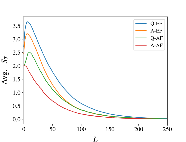
Figure 21: Four types of averages from stabilizer simulations for $T=8$, $p=0.8$. The first letter being either Q or A indicates whether the average is quenched or annealed, respectively. The last two letters being either EF or AF indicates whether the extreme value is computed first or the average is taken first, respectively.

Fig. 21 shows the average $S_{T}$ obtained from stabilizer simulation at measurement rate $p=0.8$, with four different ways of averaging. The labeling convention is detailed in the captions. By construction, fixing either the annealed (A) or the quenched (Q) average, the extreme-value-first (EF) curve always has higher value than the average-first (AF) curve. The results from exact $\mathcal{T}_{p}$ evolution yields either the annealed average-first (A-AF) or the quenched average-first (Q-AF) $S_{T}$. Although the precise $S_{T}$ values are different for the four types of averages, the resulting decay scale is the same regardless of which average is taken.

Appendix D Temporal Entanglement Profile as Bath Size Increases

Fig. 22 shows the average $S_{T}^{(t_{i})}$ profile as a 2D plot in both space and time for $T=216$ and $p=0.3$. Even in the presence of measurements, on average, the $t_{i}$ that yields maximal $S_{T}^{(t_{i})}$ still occurs at $t_{i}=\frac{T}{3}$. This is consistent with the arguments given in IV.5.

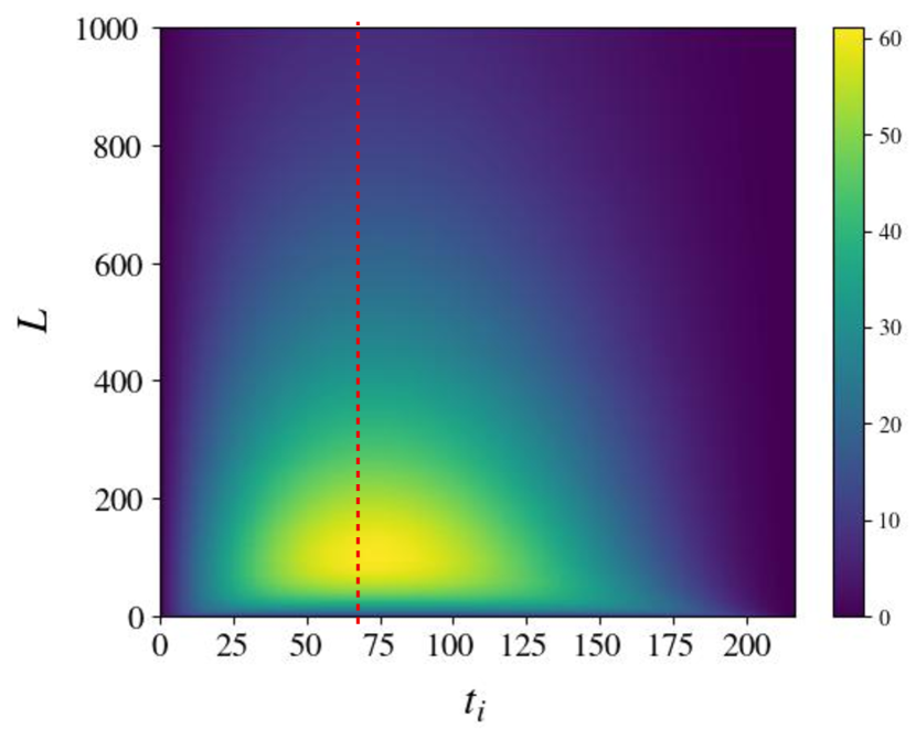
Figure 22: Average temporal entanglement profile in space and time, for total evolution time $T=216$ and measurement rate $p=0.3$. The numerical label on the color bar indicates value of the averaged temporal entanglement. The red dashed line marks the temporal cut that yields maximal average TE, which occurs on average at $t_{i}=T/3$, just like in the measurement-free case.

Appendix E Derivation of the self-consistent equation

In this Appendix we explicitly derive the self-consistent equation (92) determining the eigenvalues and momenta of the spatial transfer matrix in the single-particle sector (V). Consider the parametrization of the eigenstate $\ket{\psi}$ as

$$\psi_{j}=\begin{cases}\alpha_{+}e^{ikj}+\alpha_{-}e^{-ikj},\qquad&\textrm{for}\,j\,\textrm{even},\\ \beta_{+}e^{ikj}+\beta_{-}e^{-ikj},\qquad&\textrm{for}\,j\,\textrm{odd}.\end{cases}$$ (119)

where we take $j=0,1\dots T-1$. For $j=1,\dots,T-2$ the corresponding components of the eigenvalue equation are satisfied provided

$$\begin{bmatrix}p^{2}+J_{2}e^{-2ik}&2J_{1}\cos{k}\\ 2J_{1}\cos{k}&p^{2}+J_{2}e^{2ik}\end{bmatrix}\begin{bmatrix}\alpha_{+}\\ \beta_{+}\end{bmatrix}=\lambda\begin{bmatrix}\alpha_{+}\\ \beta_{+}\end{bmatrix},$$ (120)

and similarly

$$\begin{bmatrix}p^{2}+J_{2}e^{2ik}&2J_{1}\cos{k}\\ 2J_{1}\cos{k}&p^{2}+J_{2}e^{-2ik}\end{bmatrix}\begin{bmatrix}\alpha_{-}\\ \beta_{-}\end{bmatrix}=\lambda\begin{bmatrix}\alpha_{-}\\ \beta_{-}\end{bmatrix},$$ (121)

returning the eigenvalue $\lambda(k)$ (91). For $j=T-1$, taking $T$ even for convience, the boundary condition reads

$$\beta_{+}e^{ik(T-1)}+\beta_{-}e^{-ik(T-1)}=0,$$ (122)

whereas for $j=0$ we have that

$$p(\alpha_{+}+\alpha_{-})+(1-p)(\beta_{+}e^{ik}+\beta_{-}e^{-ik})=\lambda(k)(\alpha_{+}+\alpha_{-}).$$ (123)

Without loss of generality we can fix $\beta_{+}=e^{-ik(T-1)}$, such that the boundary condition at $j=T$ returns $\beta_{+}=-e^{ik(T-1)}$. The bulk eigenvalue equation fixes $\alpha_{\pm}$ in terms of $\beta_{\pm}$, leading to

$$\alpha_{+} =-e^{-ik(T-1)}\frac{p^{2}-\lambda(k)+J_{2}e^{2ik}}{2J_{1}\cos(k)},$$

$$\alpha_{-} =e^{ik(T-1)}\frac{p^{2}-\lambda(k)+J_{2}e^{-2ik}}{2J_{1}\cos(k)}.$$ (124)

Rewriting the boundary condition (123) as

$$\lambda(k)=p+(1-p)\frac{\beta_{+}+\beta_{-}}{\alpha_{+}+\alpha_{-}},$$ (125)

and plugging in the above expressions returns the result from the main text (92) after some straightforward manipulations. If these equations are satisfied the full state returns an eigenstate with eigenvalue $\lambda(k)$.

At $p=1/(2T)$ the value of $k$ for the leading eigenvalue changes from purely imaginary to purely real, with $k=0$ exactly at $p=1/(2T)$. For $k=0$ the eigenvalue (91) evaluates to $\lambda=(1-2p)^{2}$, and plugging this expression in the self-consistent equation (92) fixes $T=1/(2p)$. At this point the wave function of the leading eigenvalue is exactly linear, which follows as a linearization of Eq. (119) in the limit $k\to 0$. The corresponding unnormalized eigenstates are given by

$$\psi_{j}=\begin{cases}T+j,\qquad&\textrm{for}\,j\,\textrm{even},\\ T-j-1,\qquad&\textrm{for}\,j\,\textrm{odd}.\end{cases}$$ (126)

as can be verified by direct calculation.

References

- Bharti et al. [2022] K. Bharti, A. Cervera-Lierta, T. H. Kyaw, T. Haug, et al., Noisy intermediate-scale quantum algorithms, Rev. Modern Phys. 94, 015004 (2022).
- Satzinger et al. [2021] K. J. Satzinger, Y.-J. Liu, A. Smith, C. Knapp, et al., Realizing topologically ordered states on a quantum processor, Science 374, 1237 (2021).
- Mi et al. [2022] X. Mi, M. Ippoliti, C. Quintana, A. Greene, et al., Time-crystalline eigenstate order on a quantum processor, Nature 601, 531 (2022).
- Smith et al. [2019] A. Smith, M. S. Kim, F. Pollmann, and J. Knolle, Simulating quantum many-body dynamics on a current digital quantum computer, npj Quantum Inf. 5, 1 (2019).
- Liu et al. [2022] Y.-J. Liu, K. Shtengel, A. Smith, and F. Pollmann, Methods for Simulating String-Net States and Anyons on a Digital Quantum Computer, PRX Quantum 3, 040315 (2022).
- Jobst et al. [2022] B. Jobst, A. Smith, and F. Pollmann, Finite-depth scaling of infinite quantum circuits for quantum critical points, Phys. Rev. Research 4, 033118 (2022).
- Lin et al. [2021] S.-H. Lin, R. Dilip, A. G. Green, A. Smith, and F. Pollmann, Real- and Imaginary-Time Evolution with Compressed Quantum Circuits, PRX Quantum 2, 010342 (2021).
- Bertini et al. [2019a] B. Bertini, P. Kos, and T. Prosen, Exact Correlation Functions for Dual-Unitary Lattice Models in 1+1 Dimensions, Phys. Rev. Lett. 123, 210601 (2019a).
- Bertini et al. [2019b] B. Bertini, P. Kos, and T. Prosen, Entanglement Spreading in a Minimal Model of Maximal Many-Body Quantum Chaos, Phys. Rev. X 9, 021033 (2019b).
- Gopalakrishnan and Lamacraft [2019] S. Gopalakrishnan and A. Lamacraft, Unitary circuits of finite depth and infinite width from quantum channels, Phys. Rev. B 100, 064309 (2019).
- Reid and Bertini [2021] I. Reid and B. Bertini, Entanglement barriers in dual-unitary circuits, Phys. Rev. B 104, 014301 (2021).
- Bertini et al. [2020] B. Bertini, P. Kos, and T. Prosen, Operator Entanglement in Local Quantum Circuits I: Chaotic Dual-Unitary Circuits, SciPost Phys. 8, 067 (2020).
- Claeys and Lamacraft [2020] P. W. Claeys and A. Lamacraft, Maximum velocity quantum circuits, Phys. Rev. Research 2, 033032 (2020).
- Piroli et al. [2020] L. Piroli, B. Bertini, J. I. Cirac, and T. Prosen, Exact dynamics in dual-unitary quantum circuits, Phys. Rev. B 101, 094304 (2020).
- Claeys and Lamacraft [2021] P. W. Claeys and A. Lamacraft, Ergodic and Nonergodic Dual-Unitary Quantum Circuits with Arbitrary Local Hilbert Space Dimension, Phys. Rev. Lett. 126, 100603 (2021).
- Flack et al. [2020] A. Flack, B. Bertini, and T. Prosen, Statistics of the spectral form factor in the self-dual kicked Ising model, Phys. Rev. Research 2, 043403 (2020).
- Li et al. [2019] Y. Li, X. Chen, and M. P. A. Fisher, Measurement-driven entanglement transition in hybrid quantum circuits, Phys. Rev. B 100, 134306 (2019).
- Li et al. [2018] Y. Li, X. Chen, and M. P. A. Fisher, Quantum Zeno effect and the many-body entanglement transition, Phys. Rev. B 98, 205136 (2018).
- Chen et al. [2020] X. Chen, Y. Li, M. P. A. Fisher, and A. Lucas, Emergent conformal symmetry in nonunitary random dynamics of free fermions, Phys. Rev. Research 2, 033017 (2020).
- Bao et al. [2020] Y. Bao, S. Choi, and E. Altman, Theory of the phase transition in random unitary circuits with measurements, Phys. Rev. B 101, 104301 (2020).
- Choi et al. [2020] S. Choi, Y. Bao, X.-L. Qi, and E. Altman, Quantum Error Correction in Scrambling Dynamics and Measurement-Induced Phase Transition, Phys. Rev. Lett. 125, 030505 (2020).
- Zabalo et al. [2020] A. Zabalo, M. J. Gullans, J. H. Wilson, S. Gopalakrishnan, D. A. Huse, and J. H. Pixley, Critical properties of the measurement-induced transition in random quantum circuits, Phys. Rev. B 101, 060301 (2020).
- Gullans and Huse [2020] M. J. Gullans and D. A. Huse, Dynamical Purification Phase Transition Induced by Quantum Measurements, Phys. Rev. X 10, 041020 (2020).
- Jian et al. [2020] C.-M. Jian, Y.-Z. You, R. Vasseur, and A. W. W. Ludwig, Measurement-induced criticality in random quantum circuits, Phys. Rev. B 101, 104302 (2020).
- Cao et al. [2019] X. Cao, A. Tilloy, and A. De Luca, Entanglement in a fermion chain under continuous monitoring, SciPost Phys. 7, 024 (2019).
- Alberton et al. [2021] O. Alberton, M. Buchhold, and S. Diehl, Entanglement Transition in a Monitored Free-Fermion Chain: From Extended Criticality to Area Law, Phys. Rev. Lett. 126, 170602 (2021).
- Lunt and Pal [2020] O. Lunt and A. Pal, Measurement-induced entanglement transitions in many-body localized systems, Phys. Rev. Research 2, 043072 (2020).
- Paeckel et al. [2019] S. Paeckel, T. Köhler, A. Swoboda, S. R. Manmana, U. Schollwöck, and C. Hubig, Time-evolution methods for matrix-product states, Ann. Physics 411, 167998 (2019).
- Cazalilla and Marston [2002] M. A. Cazalilla and J. B. Marston, Time-Dependent Density-Matrix Renormalization Group: A Systematic Method for the Study of Quantum Many-Body Out-of-Equilibrium Systems, Phys. Rev. Lett. 88, 256403 (2002).
- White and Feiguin [2004] S. R. White and A. E. Feiguin, Real-Time Evolution Using the Density Matrix Renormalization Group, Phys. Rev. Lett. 93, 076401 (2004).
- Daley et al. [2004] A. J. Daley, C. Kollath, U. Schollwöck, and G. Vidal, Time-dependent density-matrix renormalization-group using adaptive effective Hilbert spaces, J. Stat. Mech: Theory Exp. 2004, P04005 (2004).
- Verstraete et al. [2004] F. Verstraete, J. J. García-Ripoll, and J. I. Cirac, Matrix Product Density Operators: Simulation of Finite-Temperature and Dissipative Systems, Phys. Rev. Lett. 93, 207204 (2004).
- Vidal [2003] G. Vidal, Efficient Classical Simulation of Slightly Entangled Quantum Computations, Phys. Rev. Lett. 91, 147902 (2003).
- Calabrese and Cardy [2005] P. Calabrese and J. Cardy, Evolution of entanglement entropy in one-dimensional systems, J. Stat. Mech: Theory Exp. 2005, P04010 (2005).
- Schuch et al. [2008] N. Schuch, M. M. Wolf, F. Verstraete, and J. I. Cirac, Entropy Scaling and Simulability by Matrix Product States, Phys. Rev. Lett. 100, 030504 (2008).
- Osborne [2006] T. J. Osborne, Efficient Approximation of the Dynamics of One-Dimensional Quantum Spin Systems, Phys. Rev. Lett. 97, 157202 (2006).
- Bañuls et al. [2009] M. C. Bañuls, M. B. Hastings, F. Verstraete, and J. I. Cirac, Matrix Product States for Dynamical Simulation of Infinite Chains, Phys. Rev. Lett. 102, 240603 (2009).
- Orús [2014] R. Orús, A practical introduction to tensor networks: Matrix product states and projected entangled pair states, Ann. Phys. 349, 117 (2014).
- Müller-Hermes et al. [2012] A. Müller-Hermes, J. I. Cirac, and M. C. Bañuls, Tensor network techniques for the computation of dynamical observables in one-dimensional quantum spin systems, New J. Phys. 14, 075003 (2012).
- Hastings and Mahajan [2015] M. B. Hastings and R. Mahajan, Connecting entanglement in time and space: Improving the folding algorithm, Phys. Rev. A 91, 032306 (2015).
- Feynman and Vernon [1963] R. P. Feynman and F. L. Vernon, The theory of a general quantum system interacting with a linear dissipative system, Ann. Physics 24, 118 (1963).
- Lerose et al. [2021a] A. Lerose, M. Sonner, and D. A. Abanin, Influence Matrix Approach to Many-Body Floquet Dynamics, Phys. Rev. X 11, 021040 (2021a).
- Pollock et al. [2018] F. A. Pollock, C. Rodríguez-Rosario, T. Frauenheim, M. Paternostro, and K. Modi, Non-Markovian quantum processes: Complete framework and efficient characterization, Phys. Rev. A 97, 012127 (2018).
- Strathearn et al. [2018] A. Strathearn, P. Kirton, D. Kilda, J. Keeling, and B. W. Lovett, Efficient non-Markovian quantum dynamics using time-evolving matrix product operators, Nat. Commun. 9, 3322 (2018).
- Gribben et al. [2022] D. Gribben, A. Strathearn, G. E. Fux, P. Kirton, and B. W. Lovett, Using the Environment to Understand non-Markovian Open Quantum Systems, Quantum 6, 847 (2022).
- Klobas et al. [2021] K. Klobas, B. Bertini, and L. Piroli, Exact Thermalization Dynamics in the “Rule 54” Quantum Cellular Automaton, Phys. Rev. Lett. 126, 160602 (2021).
- Lerose et al. [2021b] A. Lerose, M. Sonner, and D. A. Abanin, Scaling of temporal entanglement in proximity to integrability, Phys. Rev. B 104, 035137 (2021b).
- Giudice et al. [2022] G. Giudice, G. Giudici, M. Sonner, J. Thoenniss, A. Lerose, D. A. Abanin, and L. Piroli, Temporal Entanglement, Quasiparticles, and the Role of Interactions, Phys. Rev. Lett. 128, 220401 (2022).
- Thoenniss et al. [2023a] J. Thoenniss, M. Sonner, A. Lerose, and D. A. Abanin, Efficient method for quantum impurity problems out of equilibrium, Phys. Rev. B 107, L201115 (2023a).
- Kloss et al. [2023] B. Kloss, J. Thoenniss, M. Sonner, A. Lerose, M. T. Fishman, E. M. Stoudenmire, O. Parcollet, A. Georges, and D. A. Abanin, Equilibrium quantum impurity problems via matrix product state encoding of the retarded action, Phys. Rev. B 108, 205110 (2023).
- Thoenniss et al. [2023b] J. Thoenniss, A. Lerose, and D. A. Abanin, Nonequilibrium quantum impurity problems via matrix-product states in the temporal domain, Phys. Rev. B 107, 195101 (2023b).
- Foligno et al. [2023a] A. Foligno, T. Zhou, and B. Bertini, Temporal Entanglement in Chaotic Quantum Circuits, Phys. Rev. X 13, 041008 (2023a).
- Tirrito et al. [2022] E. Tirrito, N. J. Robinson, M. Lewenstein, S.-J. Ran, and L. Tagliacozzo, Characterizing the quantum field theory vacuum using temporal matrix product states, arXiv:1810.08050 (2022).
- Carignano et al. [2023] S. Carignano, C. R. Marimón, and L. Tagliacozzo, On temporal entropy and the complexity of computing the expectation value of local operators after a quench, arXiv:2307.11649 (2023).
- Sonner et al. [2021] M. Sonner, A. Lerose, and D. A. Abanin, Influence functional of many-body systems: Temporal entanglement and matrix-product state representation, Ann. Physics 435, 168677 (2021).
- Lerose et al. [2023] A. Lerose, M. Sonner, and D. A. Abanin, Overcoming the entanglement barrier in quantum many-body dynamics via space-time duality, Phys. Rev. B 107, L060305 (2023).
- Vidal [2004] G. Vidal, Efficient Simulation of One-Dimensional Quantum Many-Body Systems, Phys. Rev. Lett. 93, 040502 (2004).
- Sommers et al. [2023] G. M. Sommers, D. A. Huse, and M. J. Gullans, Crystalline Quantum Circuits, PRX Quantum 4, 030313 (2023).
- Akila et al. [2016] M. Akila, D. Waltner, B. Gutkin, and T. Guhr, Particle-time duality in the kicked Ising spin chain, J. Phys. Math. Theor. 49, 375101 (2016).
- Gutkin et al. [2020] B. Gutkin, P. Braun, M. Akila, D. Waltner, and T. Guhr, Exact local correlations in kicked chains, Phys. Rev. B 102, 174307 (2020).
- Ho and Choi [2022] W. W. Ho and S. Choi, Exact Emergent Quantum State Designs from Quantum Chaotic Dynamics, Phys. Rev. Lett. 128, 060601 (2022).
- Wilming and Roth [2022] H. Wilming and I. Roth, High-temperature thermalization implies the emergence of quantum state designs, arXiv:2202.01669 (2022).
- Aaronson and Gottesman [2004] S. Aaronson and D. Gottesman, Improved simulation of stabilizer circuits, Phys. Rev. A 70, 052328 (2004).
- Ippoliti et al. [2022] M. Ippoliti, T. Rakovszky, and V. Khemani, Fractal, Logarithmic, and Volume-Law Entangled Nonthermal Steady States via Spacetime Duality, Phys. Rev. X 12, 011045 (2022).
- Crooks [2020] G. E. Crooks, Gates, states, and circuits, Gates states and circuits (2020).
- Bertini et al. [2023a] B. Bertini, P. Kos, and T. Prosen, Localised Dynamics in the Floquet Quantum East Model, arXiv:2306.12467 (2023a).
- Bertini et al. [2023b] B. Bertini, C. De Fazio, J. P. Garrahan, and K. Klobas, Exact quench dynamics of the Floquet quantum East model at the deterministic point, arXiv:2310.06128 (2023b).
- Yu et al. [2023] X.-H. Yu, Z. Wang, and P. Kos, Hierarchical generalization of dual unitarity, arXiv:2307.03138 (2023).
- Rampp et al. [2023] M. A. Rampp, S. A. Rather, and P. W. Claeys, The entanglement membrane in exactly solvable lattice models, arXiv:2312.12509 (2023).
- Foligno et al. [2023b] A. Foligno, P. Kos, and B. Bertini, Quantum information spreading in generalised dual-unitary circuits, arXiv:2312.02940 (2023b).
- Sommers et al. [2024] G. M. Sommers, S. Gopalakrishnan, M. J. Gullans, and D. A. Huse, Zero-temperature entanglement membranes in quantum circuits, arXiv:2404.02975 (2024).
- Ippoliti and Khemani [2021] M. Ippoliti and V. Khemani, Postselection-Free Entanglement Dynamics via Spacetime Duality, Phys. Rev. Lett. 126, 060501 (2021).
- Lu and Grover [2021] T.-C. Lu and T. Grover, Spacetime duality between localization transitions and measurement-induced transitions, PRX Quantum 2, 040319 (2021).
- Garratt and Chalker [2021] S. Garratt and J. Chalker, Local Pairing of Feynman Histories in Many-Body Floquet Models, Phys. Rev. X 11, 021051 (2021).
- Kos et al. [2021] P. Kos, B. Bertini, and T. Prosen, Correlations in Perturbed Dual-Unitary Circuits: Efficient Path-Integral Formula, Phys. Rev. X 11, 011022 (2021).
- Knill [1996] E. Knill, Non-binary unitary error bases and quantum codes, Tech. Rep. LA-UR-96-2717 (Los Alamos National Lab. (LANL), Los Alamos, NM (United States), 1996).
- Claeys et al. [2022] P. W. Claeys, M. Henry, J. Vicary, and A. Lamacraft, Exact dynamics in dual-unitary quantum circuits with projective measurements, Phys. Rev. Research 4, 043212 (2022).
- Claeys and Lamacraft [2022] P. W. Claeys and A. Lamacraft, Emergent quantum state designs and biunitarity in dual-unitary circuit dynamics, Quantum 6, 738 (2022).
- Ippoliti and Ho [2023] M. Ippoliti and W. W. Ho, Dynamical Purification and the Emergence of Quantum State Designs from the Projected Ensemble, PRX Quantum 4, 030322 (2023).
- Claeys et al. [2023] P. W. Claeys, A. Lamacraft, and J. Vicary, From dual-unitary to biunitary: a 2-categorical model for exactly-solvable many-body quantum dynamics, arXiv:2302.07280 (2023).
- Nahum et al. [2021] A. Nahum, S. Roy, B. Skinner, and J. Ruhman, Measurement and Entanglement Phase Transitions in All-To-All Quantum Circuits, on Quantum Trees, and in Landau-Ginsburg Theory, PRX Quantum 2, 010352 (2021).
- Fidkowski et al. [2021] L. Fidkowski, J. Haah, and M. B. Hastings, How Dynamical Quantum Memories Forget, Quantum 5, 382 (2021).
- Kac [1974] M. Kac, A Stochastic Model Related to the Telegrapher’s Equation, Rocky Mountain J. Math. 4, 497 (1974).
- Berg [2004] H. C. Berg, E. coli in Motion (Springer Science & Business Media, 2004).
- Bender and Boettcher [1998] C. M. Bender and S. Boettcher, Real Spectra in Non-Hermitian Hamiltonians Having pt Symmetry, Phys. Rev. Lett. 80, 5243 (1998).
- Bender [2007] C. M. Bender, Making sense of non-Hermitian Hamiltonians, Rep. Progr. Phys. 70, 947 (2007).
- Heiss [2012] W. D. Heiss, The physics of exceptional points, J. Phys. Math. Theor. 45, 444016 (2012).
- Ashida et al. [2020] Y. Ashida, Z. Gong, and M. Ueda, Non-Hermitian physics, Adv. Phys. 69, 249 (2020).
- Bergholtz et al. [2021] E. J. Bergholtz, J. C. Budich, and F. K. Kunst, Exceptional topology of non-Hermitian systems, Rev. Modern Phys. 93, 015005 (2021).
- Yao and Wang [2018] S. Yao and Z. Wang, Edge states and topological invariants of non-hermitian systems, Phys. Rev. Lett. 121, 086803 (2018).
- Zhang et al. [2022] X. Zhang, T. Zhang, M.-H. Lu, and Y.-F. Chen, A review on non-Hermitian skin effect, Adv. Phys. 7, 2109431 (2022).