Abstract

In this study, we present an analysis of the fine-tuning required in various inflationary models in order to explain the production of Primordial Black Holes (PBHs). We specifically examine the degree of fine-tuning necessary in two prominent single field inflationary models: those with an inflection point and those with step-like features in the potential. Our findings indicate that models with step-like features generally require less fine-tuning compared to those with an inflection point, making them more viable for consistent PBH production. An interesting outcome of these models is that, in addition to improved fine-tuning, they may also predict low-frequency signals that can be detected by pulsar timing array (PTA) collaborations. Additionally, we extend our analysis to multifield inflationary models to assess whether the integration of additional fields can further alleviate the fine-tuning demands. The study also explores the role of a spectator field and its impact on the fine-tuning process. Through a comparative analysis across these models, we evaluate their parametric sensitivities and alignment with the constraints from Cosmic Microwave Background (CMB) observations. Our results indicate that although mechanisms involving a spectator field can circumvent the issue of fine-tuning parameters for PBH production, both multifield models and models with step-like features present promising alternatives. While fine-tuning involves multiple considerations, our primary objective is to evaluate various inflationary models to identify the one that most naturally explains the formation of PBHs. Hence, this study aims to the development of less constrained inflationary scenarios that align with observational data and support the theoretical possibility of PBH production.

1 Introduction

In recent years, there has been an increasing focus on primordial black holes (PBHs) due to their possible contribution to explain the dark matter of the Universe. This explanation has gained significant attention following the detection of gravitational waves (GWs) emitted by binary black hole mergers, as reported by the LIGO/VIRGO/Kagra (LVK) collaboration [1, 2, 3, 4, 5]. Moreover, the recent detection of GWs at nano-Hertz frequencies by pulsar timing array (PTA) collaborations [6, 7, 8, 9, 10, 11, 12] has sparked additional interest in the potential link between these low-frequency GWs and PBHs . Consequently, numerous theoretical studies have explored the potential link between dark matter, PBHs and GWs [13, 14, 15, 16, 17, 18, 19]. All these studies must adhere to the observational constraints on inflation from Cosmic Microwave Background (CMB) anisotropies as reported by the Planck collaboration [20, 21].

In previous theoretical researches, it is suggested that PBHs can form through a significant enhancement of the curvature perturbations at small scales. One widely adopted mechanism for producing PBHs from inflation involves studying an inflection point in the effective scalar potential [22, 23, 24, 25, 26, 27, 28, 29, 30, 31, 32, 33, 34, 35, 36]. Such inflationary potentials are generally characterized by a slow-roll phase at large scales exit the horizon, followed by an inflection point region at small scales where the power spectrum undergoes a significant enhancement. However, a major drawback of this mechanism is the high level of fine-tuning required for the parameters to achieve such a configuration in the potential [27, 23, 37].

Alternative mechanisms within the framework of single field inflation have also been proposed to alleviate the problematic fine-tuning [38, 39, 40, 41, 42, 43, 44, 45, 46, 47]. Mechanisms involving step-like features in potentials have been studied [38, 40, 41, 42]. These mechanisms can lead to a significant enhancement of the power spectrum, which is capable of explaining the production of PBHs. Interestingly, this mechanism predicts additional oscillatory patterns in the power spectra, that may lead to a characteristic signal in the induced GWs [48].

The study of an amplification of scalar power spectrum has been extend also to multi-field models. Multi-field inflationary models have been widely explored for the production of PBHs [49, 50, 51, 52, 53, 54, 55, 56, 57, 58, 59]. Models with a non-canonical kinetic term in the Lagrangian can lead to a significant enhancement in the scalar power spectrum [53, 54, 55, 56, 57, 58, 59]. Moreover, multi-field models within the framework of natural inflation, such as those involving multiple axion fields [50, 51], have been shown to result in a significant fractional abundance of PBHs. Finally, hybrid models with a waterfall trajectory are acquired a lot of interest as they provide a more natural explanation to PBHs [60, 61, 62, 63, 64, 65].

Furthermore, mechanisms involving a spectator field have been extensively explored as promising alternatives to mitigate the fine-tuning required for PBH production [66, 67, 68, 69, 70, 71, 72, 73]. Although the spectator field does not drive inflation, it evolves independently and significantly influences the formation of structures and phenomena, including PBHs. Notably, it has been demonstrated that these models can circumvent the need for fine-tuning the potential’s parameters to facilitate PBH production [67, 68].

This paper explores a diverse array of mechanisms proposed for the production of PBHs, as studied in recent literature. First, we delve into single field inflation models, examining both the inflection point mechanism and models that feature step-like characteristics, while evaluating the associated fine-tuning demands. We found that the amount of fine-tuning required for models with an inflection point is significantly large, whereas the step-like mechanism can lead to a more natural explanation as the amount of fine-tuning is significantly reduced. Notably, this mechanism can explain GW signals at low frequencies. We discuss this implementation in a separated section and leave the details for a future paper.

In the continuation of our analysis, we extend our study to multifield inflationary models. Specifically, we explore two-field model mechanisms: the first incorporates non-canonical kinetic terms in the Lagrangian, and the second features a waterfall trajectory typical of hybrid inflationary models. We find that the amount of fine-tuning is significantly reduced in both multifield mechanisms by at least three orders of magnitude in comparison with inflection point models. Lastly, we discuss the implications of models that include a spectator field for explaining the production of PBHs, highlighting that the need for fine-tuning to describe such structures can be avoided.

The layout of this paper is as follows: In Section 2, we describe our methodology for computing the amount of fine-tuning. In Section 3, we present an analysis of fine-tuning in single field inflationary mechanisms. In Section 4, we extend this analysis to two-field models. In Section 5, we discuss the amount of fine-tuning in models with a spectator field. In Section 6, we explore an interesting application of step-like potentials to scalar-induced GWs. Finally, in Section 7, we present our conclusions.

2 Fine-tuning

In this study, we focus on evaluating the degree of fine-tuning required by various mechanisms to explain the production of PBHs. It is important to note that there are several aspects of fine-tuning that need consideration. However, our primary goal is to assess different inflationary mechanisms to determine which can provide a more natural explanation for PBH formation.

To assess the fine-tuning of parameters, we employ the quantity $\Delta_{p_{i}}$, defined as the maximum value of the following logarithmic derivative [74]:

$$\Delta_{p_{i}}^{Q}=\mathrm{Max}\left|\frac{\partial\ln(Q)}{\partial\ln(p_{i})}\right|$$ (1)

Here, $Q$ represents the quantity under study, specifically the peak value of the scalar power spectrum denoted as $P_{R}^{peak}$, and $p_{i}$ denotes the corresponding parameters of each model being analyzed. This metric, $\Delta_{p_{i}}^{Q}$, quantifies the sensitivity of the observable $Q$ to variations in parameter $p_{i}$, thus serving as a measure of the required fine-tuning. A high value of $\Delta_{p_{i}}^{Q}$ implies that minor changes in $p_{i}$ result in significant alterations in $Q$, indicating a high degree of fine-tuning within the model.

We need to remark here that throughout this work, we use reduced Planck mass units, setting $\rm{M_{P}=1}$.

3 Single field models

In this section, we discuss single field inflationary models for the production of PBHs. These models are widely recognized in the literature for their role in the formation of PBHs and offer several advantages. First, they provide a simple mechanism for producing PBHs during inflation. Second, they can explain a significant fraction of dark matter. Third, they are easily adaptable to various theoretical frameworks.

In the subsequent sections, we will explore two distinct mechanisms. The first involves a mechanism characterized by an inflection point in the scalar potential [22, 23, 24, 25, 26, 27, 28, 29, 30, 31, 32, 33, 34, 35, 36]. The second examines models that incorporate step-like features [40, 41]. We compute the amount of fine-tuning for both these two different mechanism. Our result suggest that models with step-like can significantly reduce this required tuning of the parameters.

3.1 Inflection Point

3.1.1 Description of the mechanism

Significant peaks in the scalar power spectrum, which are indicative of the production of PBHs and GWs, can be generated by a near inflection point in the scalar potential. This inflection point is characterized by the conditions:

$$\begin{split}&\frac{dV(\phi_{\text{inf}})}{d\phi_{\text{inf}}}\approx 0,\quad\frac{d^{2}V(\phi_{\text{inf}})}{d\phi_{\text{inf}}^{2}}=0,\end{split}$$ (2)

where $\phi_{\text{inf}}$ denotes the inflection point. At this point, the velocity of the inflaton field significantly decreases, leading to a local enhancement while the inflaton field remains almost constant. During this plateau, the power spectrum experiences significant enhancement, facilitating the production of PBHs. In this work, we also include in this category models with bump features in the potential, such as those in [75, 33, 76], since they satisfy the conditions given in Eq.(2).

As we mentioned before, the concept of an inflection point in the potential has been widely adopted in theoretical studies. The degree of fine-tuning required for inflection point models has been extensively analyzed, notably in Ref. [37]. According to this study, polynomial potentials appear to require substantial fine-tuning both to explain the formation of PBHs and to meet the observational constraints of inflation at CMB scales.

3.1.2 The issue of fine-tuning

Among the various models proposing an inflection point, we focus on the one detailed in Ref. [22]. This model is also highlighted in Ref. [37] as one of the models requiring minimal fine-tuning within the inflection point framework. The potential, as described in Ref. [22], is given by:

$$V(\phi)=\frac{\lambda}{12}\phi^{2}\upsilon^{2}\left(\frac{6-4a\frac{\phi}{\upsilon}+3\frac{\phi^{2}}{\upsilon^{2}}}{\left(1+b\frac{\phi^{2}}{\upsilon^{2}}\right)^{2}}\right)$$ (3)

Here, $a$, $b$, $\lambda$, and $\upsilon$ are the parameters of the model. The parameter $\lambda$ sets the scale of the power spectrum at CMB scales, while the others primarily determine the shape of the potential. A significant enhancement of the power spectrum, capable of facilitating the production of PBHs, can be achieved with the following specific selection of parameters:

$$a=1/\sqrt{2},\quad b=2/3,\quad\lambda=1.86\times 10^{-6},\quad\upsilon=0.19669$$ (4)

and for initial condition we assume $\phi_{ic}=2.4719$ . This choice of initial condition lead to the following prediction of spectral index, $\rm{n_{s}}$, and tensor-to-scalar ration, $\rm{r}$:

$$n_{s}=0.956,\quad r=0.0064\,.$$ (5)

In Fig. 1, we depict the power spectrum for a small variation of the parameter $b$, which influences the inflection point and consequently requires more fine-tuning. This figure clearly demonstrates that the peak value is highly sensitive to variations in this parameter.

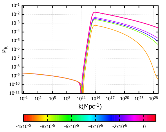
Figure 1: The power spectrum derived from the potential described in Eq. (3), showing the effects of small variations in the parameter b of order $\mathcal{O}(10^{-6})$.

To systematically quantify the fine-tuning, we evaluate the quantity of Eq. (1). In Table 1, we present the evaluation of Eq. (1) for the potential (3). Our results are consistent with those proposed by Cole et al. [37] in their study of fine-tuning for the peak of the scalar power spectrum. The parameter $\rm b$ can be given by the parameter $\rm a$ by the following expression[22, 37]:

$$b=1-\frac{a^{2}}{3}+\frac{a^{2}}{3}\left(\frac{9}{2a^{2}}-1\right)^{2/3}\,.$$ (6)

This parameter defines the inflection point. In contrast to [37], we also evaluate the fine-tuning of the parameter $\rm b$ individually, raising questions about the necessity of redefining this function and uncovering hidden fine-tuning and we found that this parameter need a lot of fine-tuning. As discussed in [37], the amount of fine-tuning required for models with an inflection point is significant; with variations in the studied models, it can reach an order of magnitude as high as $\rm{10^{8}}$. The fine-tuning associated with models featuring an inflection point has also been studied in [27, 28].

Parameter	$\Delta_{p_{i}}^{P_{R}^{peak}}$
a	$\rm{7.1\times 10^{2}}$
$\upsilon$	$\rm{4.6\times 10^{2}}$
b	$\rm{4.2\times 10^{5}}$

Table 1: Analysis of fine-tuning for the potential given in Eq. (3).

In our analysis, we also evaluate the degree of fine-tuning required for the fractional abundance of PBHs, denoted as $f\rm{{}_{PBH}}$. So, we compute the $\Delta_{p_{i}}^{f_{\rm{PBH}}}$ from Eq.(1). We found that

$${\Delta_{p_{i}}^{f_{\rm{PBH}}}}/{\Delta_{p_{i}}^{P_{R}^{peak}}}\approx 30$$ (7)

which indicates that achieving the desired fractional abundance necessitates fine-tuning that is one-two order of magnitudes more stringent than that required for the parameters outlined in Table 1. This elevated level of fine-tuning underscores the sensitivity of PBH formation to the specific dynamics of the inflationary model parameters.

3.2 Step-like potential

3.2.1 An alternative single field mechanism

In the pursuit of models that require minimal fine-tuning, the step-like potential emerges as a promising approach in single field inflationary theories [40, 41]. This potential reads as:

$$V(\varphi)=V_{0}\left(1+\frac{1}{2}\sum_{i}A_{i}\left(1+\tanh\left[c_{i}\left(\varphi-\varphi_{i}\right)\right]\right)\right)\,,$$ (8)

where $V_{0}$ is fixed for the requirement of the amplitude of power spectrum at CMB scales and $A_{i}$, $c_{i}$, and $\varphi_{i}$ are parameters that define the amplitude, steepness, and position of the steps, respectively. These steps introduce localized features in the potential, enabling significant enhancements in the scalar power spectrum.

A step-like feature in the inflaton potential results in a rapid decrease of potential energy and leads to spectral distortions [40, 41, 77]. Such features, where the potential energy abruptly transitions from one constant value to another at one or more points, can significantly enhance the spectrum over a specific range of scales.

3.2.2 Studying the fine-tuning

The potential described in Eq. (8) can be integrated into the $\alpha$-attractor framework of supergravity[41]. In our study we have the following form that adheres to the observable constraints of inflation:

$$V=(1-e^{-d\varphi})^{2}\left(V_{0}+\sum_{i=0}^{N}B_{i}\left(-1+\tanh[c(\varphi-\varphi_{i})]\right)\right)$$ (9)

where $\rm{V_{0}}$, $\rm{c}$, $\rm{d}$ and $\rm{\varphi_{i}}$ are parameters. The parameter $\rm{V_{0}}$ ensures that the potential respect the CMB constraints of inflation and the others identify the steepness and the position of the step as previously.

In this study, we focus on the potential given in Eq. (9) to explore a substantial enhancement of the scalar power spectrum. The following parameters are proposed to achieve such an enhancement at $\mathcal{O}(10^{-2})$ orders of magnitude:

$$\begin{split}V_{0}=&4\times 10^{-9},\quad B_{i}=0.05(V_{0}/2),\quad d=0.76\quad c=1000\\ \varphi_{0}=&0,\quad\varphi_{1}=5,\quad\varphi_{2}=5.2,\quad\varphi_{3}=5.4,\quad\varphi_{4}=5.6\quad\,.\end{split}$$ (10)

For initial condition we assume $\phi_{ic}=6$. The prediction for spectral index, $\rm{n_{s}}$, and tensor to scalar ratio, $\rm{r}$, are given respectively:

$$n_{s}=0.971,\quad r=0.0026\,$$ (11)

and they respect the observable constraints of inflation [21].

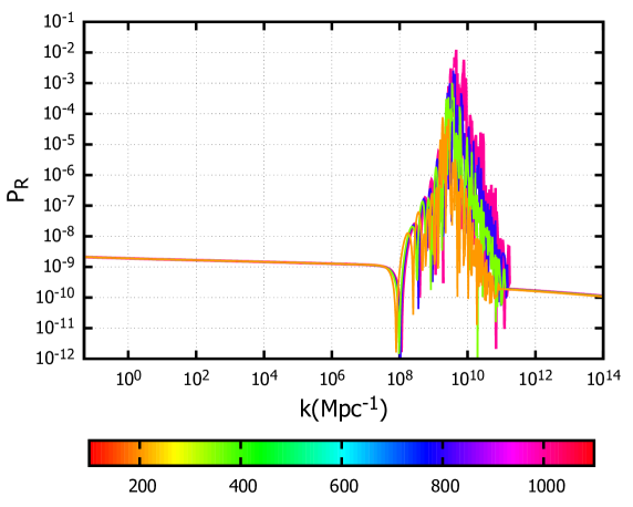
Figure 2: The power spectrum derived from the potential described in Eq. (9) for various choices of the parameter c.

The potential (9) includes four steps necessary to achieve the desired enhancement level. The dependence of the power spectrum’s peak height on the parameter $c$ is depicted in Fig. 2. The selection of this potential facilitates the formation of PBHs at $10^{-6}M_{\odot}$. However, different outcomes can be achieved by varying the choice of the parameter. A proper choice of parameters that can lead to significant results is presented in a subsequent section.

As previously described, we evaluate the parameter $\Delta_{p_{i}}^{P_{R}^{peak}}$, defined in Eq. (1), and present our findings in Table 2. We study the parameters $\rm{B_{i}}$, $\rm{c}$ and $\rm{d}$ which are responsible for the step features. We also examine the distance of the steps as $|\phi_{i+2}-\phi_{i+1}|$ where $\rm{i=0,1}$, etc. As we can notice by the Table 2, the parameter which need more fine-tuning in this case is the distances of the steps $|\phi_{i+2}-\phi_{i+1}|$. However, it is noteworthy that this mechanism exhibits a substantial reduction in the amount of fine-tuning compared to the earlier case of an inflection point in the scalar potential, see Tables 1 and 2.

Parameter	$\Delta_{p_{i}}^{P_{R}^{peak}}$
$\rm{B_{i}/V_{0}}$	$\rm{18.2}$
$\rm{c}$	$\rm{3.10}$
$\rm{d}$	$\rm{53.5}$
$|\phi_{i+2}-\phi_{i+1}|$	$\rm{80.6}$

Table 2: Analysis of fine-tuning for the potential given in Eq. (9).

4 Multi-field models

Multi-field inflationary models have been extensively studied for their role in generating PBHs. In this section, we discuss the amount of fine-tuning required in multi-field scenarios, focusing on two distinct mechanisms: one with a non-canonical kinetic term [53, 54, 55, 56, 57, 58, 59] and another with a canonical kinetic term accompanied by a waterfall trajectory [60, 61, 62, 63, 64, 65].

4.1 Two field model with a non-canonical kinetic term

In this subsection we present a two-field model featuring a non-canonical kinetic term. Although numerous mechanisms have been proposed in the literature, we specifically focus on the one detailed in Ref. [54]. The action for this two-field toy model is expressed as:

$$S=\int d^{4}x\sqrt{-g}\left[\frac{M_{P}^{2}}{2}R-\frac{1}{2}(\partial\phi)^{2}-e^{-b_{1}\phi}(\partial\chi)^{2}+V(\phi,\chi)\right]\,.$$ (12)

In this model the inflaton field $\phi$ interacts with a non-canonical scalar field $\chi$ via an exponential dilaton-like coupling [78]. The potential is defined by:

$$V(\phi,\chi)=V_{0}\frac{\phi^{2}}{\phi_{0}^{2}+\phi^{2}}+\frac{m_{\chi}^{2}}{2}\chi^{2}$$ (13)

Here $b_{1}$ is a coupling parameter between the fields and $V_{0}$, $\phi_{0}$, and $m_{\chi}$ are the model parameters. We adopt the parameter choices from [54] as follows

$$V_{0}/(m_{\chi}M_{P})^{2}=500\quad\text{and}\quad\phi_{0}=\sqrt{6}M_{P}.$$ (14)

For initial conditions we have:

$$\phi_{ic}=7,\quad\text{and}\quad\chi_{ic}=6.55$$ (15)

as they lead to acceptable values for the prediction of spectral index, $\rm{n_{s}}$, and tensor to scalar ratio, r [54, 21].

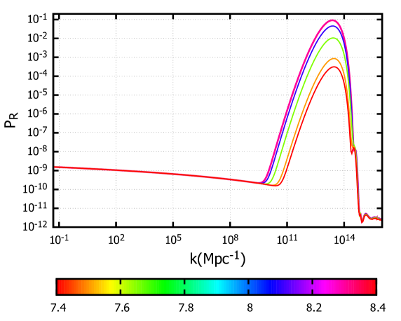
Figure 3: The power spectrum derived from the Eqs. (13) and (12) for various choices of $b_{1}$ presenting in the kinetic term.

In Fig. 3, we depict the power spectrum for various settings of the parameter $b_{1}$. It is evident that the enhancement of the power spectrum varies with the choice of this parameter. However, the impact of other parameters on the power spectrum also requires examination. Therefore, in Table 3, we present the degree of fine-tuning by evaluating Eq. (1) for all parameters, including the potential parameters $m_{\chi}$ and $\phi_{0}$. It should be noted that the parameter $V_{0}$ does not influence the dynamics of the fields, and for this reason, it is not included in this table.

Parameter	$\Delta_{p_{i}}^{P_{R}^{peak}}$
$m_{\chi}$	$\rm{1.72}$
$\rm{b_{1}}$	$\rm{71.7}$
$\rm{\phi_{0}}$	$\rm{28.7}$

Table 3: Analysis of fine-tuning for the potential given in Eqs. (13) and (12).

The results presented in Table 3 indicate that fine-tuning in multi-field inflationary models can be significantly reduced compared to single field inflationary models, particularly those with an inflection point. For a more detailed analysis, it is also essential to examine how the initial conditions of the fields may influence these results.

4.2 Hybrid model

As an additional mechanism, we study a hybrid model characterized by a waterfall trajectory. It is important to outline some fundamental aspects of this framework. The hybrid model is derived from a globally supersymmetric (SUSY) renormalizable superpotential [79, 80]:

$$W=\kappa S(\bar{\Psi}_{1}\Psi_{2}-m^{2}).$$ (16)

The $F$-term SUSY potential is given by:

$$V_{F}^{\text{SUSY}}=\kappa^{2}\left[(\psi^{2}-m^{2})^{2}+\phi^{2}\psi^{2}\right],$$ (17)

where we have set $|S|=\phi/\sqrt{2}$ and $|\Psi_{1}|=|\bar{\Psi}_{2}|=\psi$. The field $\psi$ develops tachyonic solutions under the condition:

$\kappa^{2}(-2m^{2}+\phi^{2}+6\psi^{2})<0.$

Along the flat direction ($\psi=0$), the condition becomes:

$\phi^{2}<\phi_{c}^{2}=2m^{2}\equiv M^{2},$

where $\phi_{c}$ represents the critical value of the field $\phi$, beyond which the field $\psi$ becomes tachyonic. The field $\psi$ is regarded as the waterfall field and the field $\phi$ as the inflaton.

A variety of hybrid models have been explored within the literature to elucidate the production of PBHs [60, 61, 62, 63, 64, 65]. We study the fine-tuning aspects of hybrid models, with a particular focus on the approach outlined in Ref. [62]. We selected this model due to the unique characteristics of its two-field potential, which not only serves as an attractor for the initial conditions of both fields but also ensures that, regardless of these starting conditions, the trajectory consistently leads to the potential’s plateau. Such convergence is crucial as it initiates a slow-roll phase, an important element in the dynamics of the model. The potential is given as follows:

$$V(\phi,\psi)=M^{2}\left[\frac{(\psi^{2}-\psi_{0}^{2})^{2}}{4\psi_{0}^{2}}+\frac{m^{2}}{2}\phi^{2}+\frac{g}{2}\phi^{2}\psi^{2}+d\psi\right],$$ (18)

where $M$, $m$, $g$, $d$ and $\psi_{0}$ are parameters. For the parameters we have the following

$$M=1.47\times 10^{-5},\quad m=0.3,\quad g=0.8,\quad\psi_{0}=2.5,\quad d=-5\times 10^{-6}$$ (19)

and for initial conditions

$$\phi_{ic}=3.4,\quad\psi_{ic}=0\,.$$ (20)

Hence this model align with the observable constraints of inflation [21, 62].

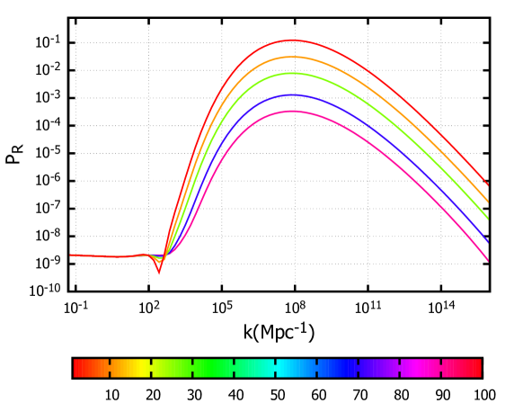
Figure 4: The power spectrum derived from the Eq. (18) for various choices of parameter $\rm{10^{6}|d|}$ .

In Fig. 4, we depict the scalar power spectrum derived from the potential in Eq. (18) for various settings of the parameter $d$. This plot illustrates that extensive fine-tuning is not necessary to achieve a significant peak in the power spectrum. As in previous mechanisms of PBHs, we analyze the impact of other parameters on the power spectrum. The parameters $m$ and $g$ influence the position of the power spectrum peak. We assess the amount of fine-tuning using Eq. (1) and present our results in Table 4.

Parameter	$\Delta_{p_{i}}^{P_{R}^{peak}}$
$m$	5.2
$g$	0.6
$d$	1.9
$\psi_{0}$	9.5

Table 4: Analysis of fine-tuning for the potential given in Eq. (18) .

As one can notice from Table 4, this mechanism significantly reduces the amount of fine-tuning required, compared to both the single field inflationary mechanism and the two-field mechanism with a non-canonical kinetic term. An important notice here is that this mechanism is not dependent on the initial condition of the fields and hence it can provide us with a more natural explanation of PBH production.

5 Spectator field

From our previous analysis, it is evident that multi-field inflationary models can significantly reduce the fine-tuning required for the production of PBHs. Additionally, the implementation of a spectator field as a solution to this issue has been extensively explored in the literature [67, 68, 69, 70], offering a promising way to circumvent the problem.

We specifically examine the model presented in Ref.[68], where the spectator field experiences quantum stochastic fluctuations. These fluctuations lead the field to assume distinct mean values across different Hubble patches. Considering the vast number of these patches, it is inevitable that some will exhibit conditions allowing the spectator field to attain values necessary for quantum fluctuations to generate significant curvature fluctuations. The potential of the spectator field is described by:

$$V(\psi)=\Lambda^{4}\left(1-\exp\left[-\frac{\psi}{M}\right]\right)$$ (21)

where $\Lambda$ and $M$ are parameters.

In this work, we further evaluate the amount of fine-tuning previously assessed to models with a spectator field. We employ the fine-tuning measure defined in Eq. (1) as we did it before. This particular mechanism does not require an enhancement in the scalar power spectrum, thereby eliminating the need to consider peaks in our evaluation. Instead, we focus on the fractional abundance of PBHs ($f_{\rm PBH}$) as our primary quantity $Q$. We specifically analyze the parameter $M$, as the parameter $\Lambda$ merely sets the scale of the spectator field and does not influence the dynamics. We found that $\Delta_{M}^{f_{\rm{PBH}}}\sim\mathcal{O}(1)$. Therefore, in this mechanism we can avoid the need of fine-tuning in order to explain the production of PBHs.

We need to remark here that the stochastic nature of the spectator field during inflation plays a crucial role in suppressing fine-tuning. In this mechanism, variations in the model’s single parameter $\rm M$, which is on the same order as the Hubble parameter at CMB scales, can be effectively compensated by the specific inflationary model we study each time. A detailed analysis can be found in [68].

6 Step-features potential over inflection-point: An additional advantage in implementation of GWs

In this section, we explore the implementation of a step-like feature potential for the production of PBHs, in comparison to models utilizing an inflection point in the potential. We demonstrate how this mechanism can not only lead to a significant enhancement and thus to copious production of PBHs, but also potentially explain the signal of GWs at low frequencies.

Figure 5: The power spectrum derived from the potential given in Eq. (9) with the choice of parameters given in (22).

To begin with, this approach facilitates a significant enhancement of the power spectrum while substantially reducing the need for fine-tuning. The reinforcement of the power spectrum is depicted in Fig. 5. For this plot we assume the following set of parameters:

$$\begin{split}c=3000,\quad d=0.73,\quad B_{i}/(V_{0}/2)=0.049,\\ |\phi_{i+2}-\phi_{i+1}|=0.2,\quad{\phi_{0}=0},\quad{\phi_{1}=5.08}\end{split}$$ (22)

and for initial condition we have $\phi_{ic}=6$. Hence the prediction of spectral index and tensor-to-scalar ratio is given as follows:

$$n_{s}=0.96839,\quad r=0.00354\,\,$$ (23)

which are in complete accordance with the observable constraints of inflation [21]. We note here that the number of efolds we obtain for this set of parameters is $N_{tot}-N_{CMB}\approx 50$, where $N_{CMB}$ denotes the number of efold at the pivot scale.

For this enhancement the mass of PBHs is about $10^{-1}M_{\odot}$ with the formalism of this evaluation presented in Appendix A.2. It is noteworthy to mention here that recently a few intriguing PBHs in low mass ratio binaries have been reported in GW observations [81, 82]. Therefore, the predicted range of masses of PBHs from this step-like mechanism can be related with the aforementioned searches and then it needs further investigation.

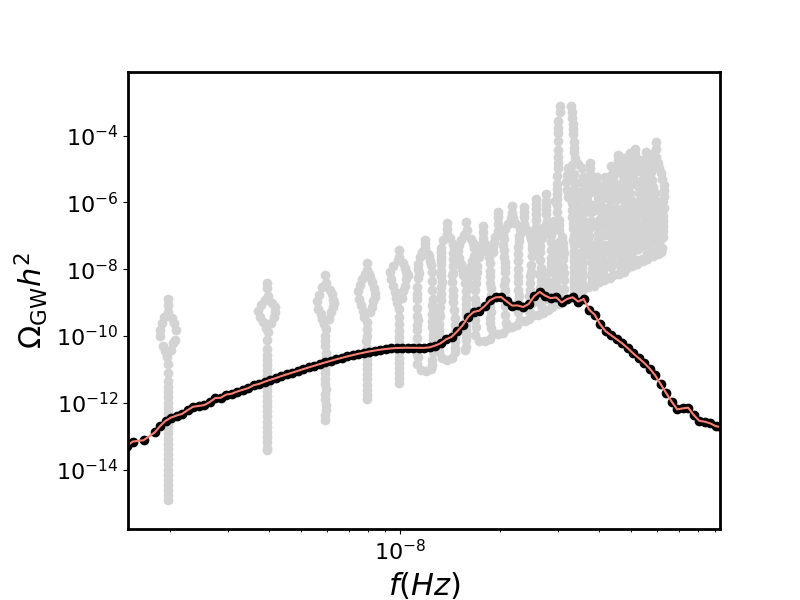
Figure 6: The energy density of GWs for the potential given in Eq. (9) with the choice of parameters given in (22).

In Fig. 6, we depict the energy density of GWs, denoted as $\Omega_{GW}$, using the specific parameters discussed in this section. The calculation of $\Omega_{GW}$ is detailed in Appendix A.3. The gray dots on the plot represent the detection sensitivity of the NANOGrav collaboration. Therefore, this mechanism has the interesting characteristic that it can be imprinted in the GW signals detected by NANOGrav [6, 7, 8].

We observe that, in addition to this enhancement, there are also additional oscillations which could be imprinted in scalar GWs, potentially leading to a characteristic signal [48, 51]. Moreover, we need to mention here that in this work we neglect possible effects of non-Gaussianities [83, 84]. Consequently, this mechanism needs further investigation and should be the focus of a future study.

7 Conclusions

This study has provided an extensive evaluation of fine-tuning requirements across various inflationary models for the production of PBHs. We have demonstrated that while single field models with inflection points require significant fine-tuning to align with CMB observations and produce PBHs, alternative models with step-like features in the scalar potential present a more favourable scenario. These models significantly reduce the need for fine-tuning and are capable of explaining the potential low-frequency GW signals detectable by PTA collaborations.

Further exploration into multi-field models reveals that the addition of extra fields can considerably alleviate the fine-tuning demands. Specifically, models incorporating non-canonical kinetic terms and hybrid inflationary models with a waterfall trajectory have shown promising results, reducing the fine-tuning requirements by orders of magnitude compared to traditional single field models.

Moreover, the implementation of a spectator field offers a novel approach to circumvent the fine-tuning issue entirely. These models allow for the natural stochastic variations in field values across different Hubble patches, which can lead to significant curvature fluctuations necessary for PBH production without the stringent constraints on the inflationary potential’s parameters.

In this work we study inflationary models in order to understand the PBH formation. These insights help expand the theoretical framework connecting inflation, dark matter, and GWs. While contributing to cosmology, this study also suggests more avenues for refining these models to enhance our understanding of their observable signatures in GWs. We acknowledge the preliminary nature of these findings and the need for further exploration to fully realize their implications.

Appendix A Appendices

A.1 Evaluation of the scalar power spectrum

In this appendix we summarise the evaluation of power spectrum which is needed in our analysis. In this framework, the field equations for ${\varphi^{i}}$, expressed in terms of efold time (assuming $\rm{M_{P}=1}$), are provided by the following equation:

$$\ddot{\varphi}^{c}+\Gamma_{ab}^{c}\dot{\varphi}^{a}\dot{\varphi}^{b}+\left(3-\frac{1}{2}\dot{\sigma^{2}}\right)\dot{\varphi}^{c}+\left(3-\frac{1}{2}\dot{\sigma^{2}}\right)\frac{V^{c}}{V}=0$$ (24)

where the dots indicate derivatives with respect to efold time, and the indices $\mathrm{i=a,b,c}$ denote derivatives relative to the fields. The Christoffel symbols $\Gamma^{c}_{ab}$ are defined as:

$$\Gamma^{c}_{ab}=\frac{1}{2}G^{cd}(G_{da,b}+G_{db,a}-G_{ab,d}),$$ (25)

where $\mathrm{G_{ij}}$ represents the field metric. The velocity field $\dot{\sigma}$ is calculated as:

$$\dot{\sigma}^{2}=G_{ab}\dot{{\varphi}^{a}}\dot{{\varphi}^{b}}.$$ (26)

The Hubble parameter is defined by:

$$H^{2}=\frac{V}{3-\frac{1}{2}\dot{\sigma^{2}}}$$ (27)

and the slow-roll parameter $\epsilon_{1}$ is determined from:

$$\epsilon_{1}=\frac{1}{2}\dot{\sigma^{2}}.$$ (28)

The perturbation equations for the fields ${\delta\varphi}$ are given by:

$$\begin{split}&\delta\ddot{\varphi}^{c}+(3-\epsilon_{1})\delta\dot{\varphi}^{c}+2\Gamma^{c}_{ab}\dot{\varphi}^{a}\delta\dot{\varphi}^{b}+\left(\Gamma^{c}_{ab,d}\dot{\varphi}^{a}\dot{\varphi}^{b}+\frac{V^{c}_{d}}{H^{2}}-G^{ca}G_{ab,d}\frac{V^{b}}{H^{2}}\right)\delta\varphi^{d}\\ &+\frac{k^{2}}{a^{2}H^{2}}\delta\varphi^{c}=4\dot{\Psi}\dot{\varphi}-2\Psi\frac{V^{c}}{H^{2}}\end{split}$$ (29)

and the equation for the Bardeen potential $\Psi$ is:

$$\ddot{\Psi}+(7-\epsilon_{1})\dot{\Psi}+\left(2\frac{V}{H^{2}}+\frac{k^{2}}{a^{2}H^{2}}\right)\Psi=-\frac{V_{c}}{H^{2}}\delta\varphi^{c}.$$ (30)

We assume the initial condition of a Bunch-Davies vacuum. The power spectrum is described by:

$$P_{R}=\frac{k^{3}}{(2\pi)^{2}}(R_{i}^{2})$$ (31)

where:

$$R_{i}=\Psi+H\sum_{i}^{N_{\text{fields}}}\frac{\dot{\varphi_{i}}\delta\varphi_{i}}{\dot{\varphi_{i}}^{2}}.$$ (32)

A.2 Evaluation of the fractional abundances of PBHs

In this appendix we briefly discuss how to evalaute the the fractional abundance of PBHs. The present abundance of PBH is given by the integral:

$$f_{PBH}=\int d\ln M_{PBH}\frac{\Omega_{PBH}}{\Omega_{DM}}$$ (33)

where

$$\frac{\Omega_{PBH}}{\Omega_{DM}}=\frac{\beta(M_{\text{PBH}}(k))}{8\times 10^{-16}}\left(\frac{\gamma}{0.2}\right)^{3/2}\left(\frac{g(T_{f})}{106.75}\right)^{-1/4}\left(\frac{M_{\text{PBH}}(k)}{10^{-18}\textsl{g}}\right)^{-1/2}.$$ (34)

Here $\gamma$ is a factor which depends on gravitation collapse and we choose $\gamma=0.2$ [85]. $T_{f}$ denotes the temperature of PBH formation and $M_{\text{PBH}}$ is the mass of PBHs. $g(T_{f})$ are the effective degrees of freedom during this formation and counting only the SM particles we set $g(T_{f})=106.75$.

The mass fraction of PBH at formation, denoted by $\beta(M_{\text{PBH}})$:

$$\beta(M_{\text{PBH}})=\frac{1}{\sqrt{2\pi\sigma^{2}(M_{\text{PBH}})}}\int^{\infty}_{\delta_{c}}d\delta\,\exp\left(-\frac{\delta^{2}}{2\sigma^{2}(M_{\text{PBH}})}\right)\,,$$ (35)

where $\delta$ denotes

$$\sigma^{2}\left(M_{\text{PBH}}(k)\right)=\frac{16}{81}\int\frac{dk^{\prime}}{k^{\prime}}\left(\frac{k^{\prime}}{k}\right)^{4}P_{\mathcal{R}}(k^{\prime})W^{2}\left(\frac{k^{\prime}}{k}\right),$$ (36)

where W is a window function.

The mass as a function of $k$ [24]:

$$M_{PBH}=10^{18}\left(\frac{\gamma}{0.2}\right)\left(\frac{g(T_{f})}{106.75}\right)^{-1/6}\left(\frac{k}{7\times 10^{13}Mpc^{-1}}\right)^{-2}\textsl{g}\,.$$ (37)

A.3 Energy Density of GWs

In this appendix we briefly discuss how to evaluate the energy density of GWs from the scalar power spectrum. The energy density of the GWs can be evaluated from the following integral  [86, 87, 88, 89, 90]

$${\Omega_{GW}(k)}=\frac{\Omega_{r}}{36}\int^{\frac{1}{\sqrt{3}}}_{0}\mathrm{d}d\int^{\infty}_{\frac{1}{\sqrt{3}}}\mathrm{d}s\left[\frac{(s^{2}-1/3)(d^{2}-1/3)}{s^{2}+d^{2}}\right]^{2}\,P_{R}(kx)\,P_{R}(ky)\,(I_{c}^{2}+I_{s}^{2}).$$ (38)

where the radiation density $\Omega_{r}\approx 5.4\times 10^{-5}$. The variables $x$ and $y$ are

$$x=\frac{\sqrt{3}}{2}(s+d),\quad y=\frac{\sqrt{3}}{2}(s-d).$$ (39)

The functions $I_{c}$ and $I_{s}$ are given by the expressions

$$I_{c}=-36\pi\frac{(s^{2}+d^{2}-2)^{2}}{(s^{2}-d^{2})^{3}}\Theta(s-1)$$ (40)

$$I_{s}=-36\frac{(s^{2}+d^{2}-2)^{2}}{(s^{2}-d^{2})^{2}}\left[\frac{(s^{2}+d^{2}-2)}{(s^{2}-d^{2})}\log\left|\frac{d^{2}-1}{s^{2}-1}\right|+2\right].$$ (41)

Using that

$1\,{\rm Mpc}^{-1}=0.97154\times\,10^{-14}\,{\rm s}^{-1}$ and $k=2\pi f$

we can evaluate the energy density of power spectrum as a function of the frequency $f$.

References

- [1] B. P. Abbott, et al., Observation of Gravitational Waves from a Binary Black Hole Merger, Phys. Rev. Lett. 116 (6) (2016) 061102. arXiv:1602.03837, doi:10.1103/PhysRevLett.116.061102.
- [2] B. P. Abbott, et al., GW151226: Observation of Gravitational Waves from a 22-Solar-Mass Binary Black Hole Coalescence, Phys. Rev. Lett. 116 (24) (2016) 241103. arXiv:1606.04855, doi:10.1103/PhysRevLett.116.241103.
- [3] B. P. Abbott, et al., GW170104: Observation of a 50-Solar-Mass Binary Black Hole Coalescence at Redshift 0.2, Phys. Rev. Lett. 118 (22) (2017) 221101, [Erratum: Phys.Rev.Lett. 121, 129901 (2018)]. arXiv:1706.01812, doi:10.1103/PhysRevLett.118.221101.
- [4] B. P. Abbott, et al., GW170608: Observation of a 19-solar-mass Binary Black Hole Coalescence, Astrophys. J. Lett. 851 (2017) L35. arXiv:1711.05578, doi:10.3847/2041-8213/aa9f0c.
- [5] B. P. Abbott, et al., GW170814: A Three-Detector Observation of Gravitational Waves from a Binary Black Hole Coalescence, Phys. Rev. Lett. 119 (14) (2017) 141101. arXiv:1709.09660, doi:10.1103/PhysRevLett.119.141101.
- [6] G. Agazie, et al., The NANOGrav 15 yr Data Set: Evidence for a Gravitational-wave Background, Astrophys. J. Lett. 951 (1) (2023) L8. arXiv:2306.16213, doi:10.3847/2041-8213/acdac6.
- [7] G. Agazie, et al., The NANOGrav 15 yr Data Set: Observations and Timing of 68 Millisecond Pulsars, Astrophys. J. Lett. 951 (1) (2023) L9. arXiv:2306.16217, doi:10.3847/2041-8213/acda9a.
- [8] A. Afzal, et al., The NANOGrav 15 yr Data Set: Search for Signals from New Physics, Astrophys. J. Lett. 951 (1) (2023) L11. arXiv:2306.16219, doi:10.3847/2041-8213/acdc91.
- [9] J. Antoniadis, et al., The second data release from the European Pulsar Timing Array - III. Search for gravitational wave signals, Astron. Astrophys. 678 (2023) A50. arXiv:2306.16214, doi:10.1051/0004-6361/202346844.
- [10] J. Antoniadis, et al., The second data release from the European Pulsar Timing Array - I. The dataset and timing analysis, Astron. Astrophys. 678 (2023) A48. arXiv:2306.16224, doi:10.1051/0004-6361/202346841.
- [11] J. Antoniadis, et al., The second data release from the European Pulsar Timing Array - II. Customised pulsar noise models for spatially correlated gravitational waves, Astron. Astrophys. 678 (2023) A49. arXiv:2306.16225, doi:10.1051/0004-6361/202346842.
- [12] J. Antoniadis, et al., The second data release from the European Pulsar Timing Array: V. Implications for massive black holes, dark matter and the early Universe (6 2023). arXiv:2306.16227.
- [13] O. Özsoy, G. Tasinato, Inflation and Primordial Black Holes, Universe 9 (5) (2023) 203. arXiv:2301.03600, doi:10.3390/universe9050203.
- [14] M. Sasaki, T. Suyama, T. Tanaka, S. Yokoyama, Primordial black holes—perspectives in gravitational wave astronomy, Class. Quant. Grav. 35 (6) (2018) 063001. arXiv:1801.05235, doi:10.1088/1361-6382/aaa7b4.
- [15] B. Carr, S. Clesse, J. Garcia-Bellido, M. Hawkins, F. Kuhnel, Observational evidence for primordial black holes: A positivist perspective, Phys. Rept. 1054 (2024) 1–68. arXiv:2306.03903, doi:10.1016/j.physrep.2023.11.005.
- [16] M. Y. Khlopov, Primordial Black Holes, Res. Astron. Astrophys. 10 (2010) 495–528. arXiv:0801.0116, doi:10.1088/1674-4527/10/6/001.
- [17] F. Kuhnel, I. Stamou, Reconstructing Primordial Black Hole Power Spectra from Gravitational Waves (4 2024). arXiv:2404.06547.
- [18] J. Ellis, M. Fairbairn, G. Franciolini, G. Hütsi, A. Iovino, M. Lewicki, M. Raidal, J. Urrutia, V. Vaskonen, H. Veermäe, What is the source of the PTA GW signal?, Phys. Rev. D 109 (2) (2024) 023522. arXiv:2308.08546, doi:10.1103/PhysRevD.109.023522.
- [19] V. Vaskonen, H. Veermäe, Did NANOGrav see a signal from primordial black hole formation?, Phys. Rev. Lett. 126 (5) (2021) 051303. arXiv:2009.07832, doi:10.1103/PhysRevLett.126.051303.
- [20] P. A. R. Ade, et al., Planck 2015 results. XX. Constraints on inflation, Astron. Astrophys. 594 (2016) A20. arXiv:1502.02114, doi:10.1051/0004-6361/201525898.
- [21] Y. Akrami, et al., Planck 2018 results. X. Constraints on inflation, Astron. Astrophys. 641 (2020) A10. arXiv:1807.06211, doi:10.1051/0004-6361/201833887.
- [22] J. Garcia-Bellido, E. Ruiz Morales, Primordial black holes from single field models of inflation, Phys. Dark Univ. 18 (2017) 47–54. arXiv:1702.03901, doi:10.1016/j.dark.2017.09.007.
- [23] M. P. Hertzberg, M. Yamada, Primordial Black Holes from Polynomial Potentials in Single Field Inflation, Phys. Rev. D 97 (8) (2018) 083509. arXiv:1712.09750, doi:10.1103/PhysRevD.97.083509.
- [24] G. Ballesteros, M. Taoso, Primordial black hole dark matter from single field inflation, Phys. Rev. D 97 (2) (2018) 023501. arXiv:1709.05565, doi:10.1103/PhysRevD.97.023501.
- [25] G. Ballesteros, J. Rey, F. Rompineve, Detuning primordial black hole dark matter with early matter domination and axion monodromy, JCAP 06 (2020) 014. arXiv:1912.01638, doi:10.1088/1475-7516/2020/06/014.
- [26] M. Cicoli, V. A. Diaz, F. G. Pedro, Primordial Black Holes from String Inflation, JCAP 06 (2018) 034. arXiv:1803.02837, doi:10.1088/1475-7516/2018/06/034.
- [27] I. D. Stamou, Mechanisms of producing primordial black holes by breaking the symmetry, Phys. Rev. D 103 (8) (2021) 083512. arXiv:2104.08654, doi:10.1103/PhysRevD.103.083512.
- [28] V. C. Spanos, I. D. Stamou, Gravitational waves from no-scale supergravity, Eur. Phys. J. C 83 (1) (2023) 4. arXiv:2205.05595, doi:10.1140/epjc/s10052-022-11142-x.
- [29] I. Dalianis, A. Kehagias, G. Tringas, Primordial black holes from -attractors, JCAP 01 (2019) 037. arXiv:1805.09483, doi:10.1088/1475-7516/2019/01/037.
- [30] C. Germani, T. Prokopec, On primordial black holes from an inflection point, Phys. Dark Univ. 18 (2017) 6–10. arXiv:1706.04226, doi:10.1016/j.dark.2017.09.001.
- [31] J. M. Ezquiaga, J. Garcia-Bellido, E. Ruiz Morales, Primordial Black Hole production in Critical Higgs Inflation, Phys. Lett. B 776 (2018) 345–349. arXiv:1705.04861, doi:10.1016/j.physletb.2017.11.039.
- [32] O. Özsoy, S. Parameswaran, G. Tasinato, I. Zavala, Mechanisms for Primordial Black Hole Production in String Theory, JCAP 07 (2018) 005. arXiv:1803.07626, doi:10.1088/1475-7516/2018/07/005.
- [33] O. Özsoy, Z. Lalak, Primordial black holes as dark matter and gravitational waves from bumpy axion inflation, JCAP 01 (2021) 040. arXiv:2008.07549, doi:10.1088/1475-7516/2021/01/040.
- [34] A. Karam, N. Koivunen, E. Tomberg, V. Vaskonen, H. Veermäe, Anatomy of single-field inflationary models for primordial black holes, JCAP 03 (2023) 013. arXiv:2205.13540, doi:10.1088/1475-7516/2023/03/013.
- [35] Y. Aldabergenov, S. V. Ketov, Primordial Black Holes from Volkov–Akulov–Starobinsky Supergravity, Fortsch. Phys. 71 (6-7) (2023) 2300039. arXiv:2301.12750, doi:10.1002/prop.202300039.
- [36] K. Kannike, L. Marzola, M. Raidal, H. Veermäe, Single Field Double Inflation and Primordial Black Holes, JCAP 09 (2017) 020. arXiv:1705.06225, doi:10.1088/1475-7516/2017/09/020.
- [37] P. S. Cole, A. D. Gow, C. T. Byrnes, S. P. Patil, Primordial black holes from single-field inflation: a fine-tuning audit, JCAP 08 (2023) 031. arXiv:2304.01997, doi:10.1088/1475-7516/2023/08/031.
- [38] K. Inomata, E. McDonough, W. Hu, Amplification of primordial perturbations from the rise or fall of the inflaton, JCAP 02 (02) (2022) 031. arXiv:2110.14641, doi:10.1088/1475-7516/2022/02/031.
- [39] E. Cotner, A. Kusenko, Primordial black holes from scalar field evolution in the early universe, Phys. Rev. D 96 (10) (2017) 103002. arXiv:1706.09003, doi:10.1103/PhysRevD.96.103002.
- [40] K. Kefala, G. P. Kodaxis, I. D. Stamou, N. Tetradis, Features of the inflaton potential and the power spectrum of cosmological perturbations, Phys. Rev. D 104 (2) (2021) 023506. arXiv:2010.12483, doi:10.1103/PhysRevD.104.023506.
- [41] I. Dalianis, G. P. Kodaxis, I. D. Stamou, N. Tetradis, A. Tsigkas-Kouvelis, Spectrum oscillations from features in the potential of single-field inflation, Phys. Rev. D 104 (10) (2021) 103510. arXiv:2106.02467, doi:10.1103/PhysRevD.104.103510.
- [42] Y.-F. Cai, X.-H. Ma, M. Sasaki, D.-G. Wang, Z. Zhou, One small step for an inflaton, one giant leap for inflation: A novel non-Gaussian tail and primordial black holes, Phys. Lett. B 834 (2022) 137461. arXiv:2112.13836, doi:10.1016/j.physletb.2022.137461.
- [43] S. Choudhury, S. Panda, M. Sami, PBH formation in EFT of single field inflation with sharp transition, Phys. Lett. B 845 (2023) 138123. arXiv:2302.05655, doi:10.1016/j.physletb.2023.138123.
- [44] S. Choudhury, A. Karde, P. Padiyar, M. Sami, Primordial Black Holes from Effective Field Theory of Stochastic Single Field Inflation at NNNLO (3 2024). arXiv:2403.13484.
- [45] B.-M. Gu, F.-W. Shu, K. Yang, Inflation with shallow dip and primordial black holes (7 2023). arXiv:2307.00510.
- [46] M. Drees, E. Erfani, Running Spectral Index and Formation of Primordial Black Hole in Single Field Inflation Models, JCAP 01 (2012) 035. arXiv:1110.6052, doi:10.1088/1475-7516/2012/01/035.
- [47] G. Domènech, G. Vargas, T. Vargas, An exact model for enhancing/suppressing primordial fluctuations, JCAP 03 (2024) 002. arXiv:2309.05750, doi:10.1088/1475-7516/2024/03/002.
- [48] J. Fumagalli, S. Renaux-Petel, L. T. Witkowski, Oscillations in the stochastic gravitational wave background from sharp features and particle production during inflation, JCAP 08 (2021) 030. arXiv:2012.02761, doi:10.1088/1475-7516/2021/08/030.
- [49] G. A. Palma, S. Sypsas, C. Zenteno, Seeding primordial black holes in multifield inflation, Phys. Rev. Lett. 125 (12) (2020) 121301. arXiv:2004.06106, doi:10.1103/PhysRevLett.125.121301.
- [50] Z. Zhou, J. Jiang, Y.-F. Cai, M. Sasaki, S. Pi, Primordial black holes and gravitational waves from resonant amplification during inflation, Phys. Rev. D 102 (10) (2020) 103527. arXiv:2010.03537, doi:10.1103/PhysRevD.102.103527.
- [51] N. E. Mavromatos, V. C. Spanos, I. D. Stamou, Primordial black holes and gravitational waves in multiaxion-Chern-Simons inflation, Phys. Rev. D 106 (6) (2022) 063532. arXiv:2206.07963, doi:10.1103/PhysRevD.106.063532.
- [52] S. Kawai, J. Kim, Primordial black holes and gravitational waves from nonminimally coupled supergravity inflation, Phys. Rev. D 107 (4) (2023) 043523. arXiv:2209.15343, doi:10.1103/PhysRevD.107.043523.
- [53] Y. Aldabergenov, A. Addazi, S. V. Ketov, Inflation, SUSY breaking, and primordial black holes in modified supergravity coupled to chiral matter, Eur. Phys. J. C 82 (8) (2022) 681. arXiv:2206.02601, doi:10.1140/epjc/s10052-022-10654-w.
- [54] M. Braglia, D. K. Hazra, F. Finelli, G. F. Smoot, L. Sriramkumar, A. A. Starobinsky, Generating PBHs and small-scale GWs in two-field models of inflation, JCAP 08 (2020) 001. arXiv:2005.02895, doi:10.1088/1475-7516/2020/08/001.
- [55] S. Pi, M. Sasaki, Primordial black hole formation in nonminimal curvaton scenarios, Phys. Rev. D 108 (10) (2023) L101301. arXiv:2112.12680, doi:10.1103/PhysRevD.108.L101301.
- [56] A. Gundhi, S. V. Ketov, C. F. Steinwachs, Primordial black hole dark matter in dilaton-extended two-field Starobinsky inflation, Phys. Rev. D 103 (8) (2021) 083518. arXiv:2011.05999, doi:10.1103/PhysRevD.103.083518.
- [57] S. R. Geller, W. Qin, E. McDonough, D. I. Kaiser, Primordial black holes from multifield inflation with nonminimal couplings, Phys. Rev. D 106 (6) (2022) 063535. arXiv:2205.04471, doi:10.1103/PhysRevD.106.063535.
- [58] C. Chen, A. Ghoshal, Z. Lalak, Y. Luo, A. Naskar, Growth of curvature perturbations for PBH formation & detectable GWs in non-minimal curvaton scenario revisited, JCAP 08 (2023) 041. arXiv:2305.12325, doi:10.1088/1475-7516/2023/08/041.
- [59] X. Wang, Y.-l. Zhang, M. Sasaki, Enhanced Curvature Perturbation and Primordial Black Hole Formation in Two-stage Inflation with a break (4 2024). arXiv:2404.02492.
- [60] A. Afzal, A. Ghoshal, Primordial Black Holes and Scalar-induced Gravitational Waves in Radiative Hybrid Inflation (2 2024). arXiv:2402.06613.
- [61] V. C. Spanos, I. D. Stamou, Gravitational waves and primordial black holes from supersymmetric hybrid inflation, Phys. Rev. D 104 (12) (2021) 123537. arXiv:2108.05671, doi:10.1103/PhysRevD.104.123537.
- [62] M. Braglia, A. Linde, R. Kallosh, F. Finelli, Hybrid -attractors, primordial black holes and gravitational wave backgrounds, JCAP 04 (2023) 033. arXiv:2211.14262, doi:10.1088/1475-7516/2023/04/033.
- [63] S. Clesse, J. García-Bellido, Massive Primordial Black Holes from Hybrid Inflation as Dark Matter and the seeds of Galaxies, Phys. Rev. D 92 (2) (2015) 023524. arXiv:1501.07565, doi:10.1103/PhysRevD.92.023524.
- [64] Y. Tada, M. Yamada, Stochastic dynamics of multi-waterfall hybrid inflation and formation of primordial black holes, JCAP 11 (2023) 089. arXiv:2306.07324, doi:10.1088/1475-7516/2023/11/089.
- [65] K. Dimopoulos, Waterfall stiff period can generate observable primordial gravitational waves, JCAP 10 (2022) 027. arXiv:2206.02264, doi:10.1088/1475-7516/2022/10/027.
- [66] B. Carr, T. Tenkanen, V. Vaskonen, Primordial black holes from inflaton and spectator field perturbations in a matter-dominated era, Phys. Rev. D 96 (6) (2017) 063507. arXiv:1706.03746, doi:10.1103/PhysRevD.96.063507.
- [67] K. Kohri, C.-M. Lin, T. Matsuda, Primordial black holes from the inflating curvaton, Phys. Rev. D 87 (10) (2013) 103527. arXiv:1211.2371, doi:10.1103/PhysRevD.87.103527.
- [68] I. Stamou, S. Clesse, Primordial black holes without fine-tuning from a light stochastic spectator field, Phys. Rev. D 109 (4) (2024) 043522. arXiv:2310.04174, doi:10.1103/PhysRevD.109.043522.
- [69] I. Stamou, S. Clesse, Can Primordial Black Holes form in the Standard Model ? (12 2023). arXiv:2312.06873.
- [70] I. D. Stamou, Large curvature fluctuations from no-scale supergravity with a spectator field (4 2024). arXiv:2404.02295.
- [71] R.-G. Cai, C. Chen, C. Fu, Primordial black holes and stochastic gravitational wave background from inflation with a noncanonical spectator field, Phys. Rev. D 104 (8) (2021) 083537. arXiv:2108.03422, doi:10.1103/PhysRevD.104.083537.
- [72] A. D. Gow, T. Miranda, S. Nurmi, Primordial black holes from a curvaton scenario with strongly non-Gaussian perturbations, JCAP 11 (2023) 006. arXiv:2307.03078, doi:10.1088/1475-7516/2023/11/006.
- [73] D. Hooper, A. Ireland, G. Krnjaic, A. Stebbins, Supermassive primordial black holes from inflation, JCAP 04 (2024) 021. arXiv:2308.00756, doi:10.1088/1475-7516/2024/04/021.
- [74] R. Barbieri, G. Giudice, Upper Bounds on Supersymmetric Particle Masses, Nucl. Phys. B 306 (1988) 63–76. doi:10.1016/0550-3213(88)90171-X.
- [75] S. S. Mishra, V. Sahni, Primordial Black Holes from a tiny bump/dip in the Inflaton potential, JCAP 04 (2020) 007. arXiv:1911.00057, doi:10.1088/1475-7516/2020/04/007.
- [76] C. Fu, C. Chen, Sudden braking and turning with a two-field potential bump: primordial black hole formation, JCAP 05 (2023) 005. arXiv:2211.11387, doi:10.1088/1475-7516/2023/05/005.
- [77] I. Dalianis, Features in the Inflaton Potential and the Spectrum of Cosmological Perturbations, 2023. arXiv:2310.11581.
- [78] R. Kallosh, A. Linde, Dilaton-axion inflation with PBHs and GWs, JCAP 08 (08) (2022) 037. arXiv:2203.10437, doi:10.1088/1475-7516/2022/08/037.
- [79] E. J. Copeland, A. R. Liddle, D. H. Lyth, E. D. Stewart, D. Wands, False vacuum inflation with Einstein gravity, Phys. Rev. D 49 (1994) 6410–6433. arXiv:astro-ph/9401011, doi:10.1103/PhysRevD.49.6410.
- [80] G. R. Dvali, Q. Shafi, R. K. Schaefer, Large scale structure and supersymmetric inflation without fine tuning, Phys. Rev. Lett. 73 (1994) 1886–1889. arXiv:hep-ph/9406319, doi:10.1103/PhysRevLett.73.1886.
- [81] R. Abbott, et al., Search for subsolar-mass black hole binaries in the second part of Advanced LIGO’s and Advanced Virgo’s third observing run, Mon. Not. Roy. Astron. Soc. 524 (4) (2023) 5984–5992, [Erratum: Mon.Not.Roy.Astron.Soc. 526, 6234 (2023)]. arXiv:2212.01477, doi:10.1093/mnras/stad588.
- [82] K. S. Phukon, G. Baltus, S. Caudill, S. Clesse, A. Depasse, M. Fays, H. Fong, S. J. Kapadia, R. Magee, A. J. Tanasijczuk, The hunt for sub-solar primordial black holes in low mass ratio binaries is open (5 2021). arXiv:2105.11449.
- [83] R.-g. Cai, S. Pi, M. Sasaki, Gravitational Waves Induced by non-Gaussian Scalar Perturbations, Phys. Rev. Lett. 122 (20) (2019) 201101. arXiv:1810.11000, doi:10.1103/PhysRevLett.122.201101.
- [84] G. Perna, C. Testini, A. Ricciardone, S. Matarrese, Fully non-Gaussian Scalar-Induced Gravitational Waves (3 2024). arXiv:2403.06962.
- [85] B. J. Carr, The Primordial black hole mass spectrum, Astrophys. J. 201 (1975) 1–19. doi:10.1086/153853.
- [86] J. R. Espinosa, D. Racco, A. Riotto, A Cosmological Signature of the SM Higgs Instability: Gravitational Waves, JCAP 09 (2018) 012. arXiv:1804.07732, doi:10.1088/1475-7516/2018/09/012.
- [87] K. Kohri, T. Terada, Semianalytic calculation of gravitational wave spectrum nonlinearly induced from primordial curvature perturbations, Phys. Rev. D 97 (12) (2018) 123532. arXiv:1804.08577, doi:10.1103/PhysRevD.97.123532.
- [88] S. Mollerach, D. Harari, S. Matarrese, CMB polarization from secondary vector and tensor modes, Phys. Rev. D 69 (2004) 063002. arXiv:astro-ph/0310711, doi:10.1103/PhysRevD.69.063002.
- [89] M. Maggiore, Gravitational wave experiments and early universe cosmology, Phys. Rept. 331 (2000) 283–367. arXiv:gr-qc/9909001, doi:10.1016/S0370-1573(99)00102-7.
- [90] D. Baumann, P. J. Steinhardt, K. Takahashi, K. Ichiki, Gravitational Wave Spectrum Induced by Primordial Scalar Perturbations, Phys. Rev. D 76 (2007) 084019. arXiv:hep-th/0703290, doi:10.1103/PhysRevD.76.084019.