Multi-Agent Hybrid Soft Actor-Critic for Joint Spectrum Sensing and Dynamic Spectrum Access in Cognitive Radio Networks

Abstract.

Opportunistic spectrum access has the potential to increase the efficiency of spectrum utilization in cognitive radio networks (CRNs). In CRNs, both spectrum sensing and resource allocation (SSRA) are critical to maximizing system throughput while minimizing collisions of secondary users with the primary network. However, many works in dynamic spectrum access do not consider the impact of imperfect sensing information such as mis-detected channels, which the additional information available in joint SSRA can help remediate. In this work, we examine joint SSRA as an optimization which seeks to maximize a CRN's net communication rate subject to constraints on channel sensing, channel access, and transmit power. Given the non-trivial nature of the problem, we leverage multi-agent reinforcement learning to enable a network of secondary users to dynamically access unoccupied spectrum via only local test statistics, formulated under the energy detection paradigm of spectrum sensing. In doing so, we develop a novel multi-agent implementation of hybrid soft actor critic, MHSAC, based on the QMIX mixing scheme. Through experiments, we find that our SSRA algorithm, HySSRA, is successful in maximizing the CRN's utilization of spectrum resources while also limiting its interference with the primary network, and outperforms the current state-of-the-art by a wide margin. We also explore the impact of wireless variations such as coherence time on the efficacy of the system.

1. Introduction

With the continued proliferation of wireless devices – having already reached approximately $30$ billion worldwide by $2023$ (Dhull et al., 2022) – the corresponding spectrum available for transmission is becoming increasingly limited. In this regard, cognitive radio networks (CRNs), proposed in (Devroye et al., 2008), offer a method for more efficient spectrum utilization. CRNs consist of primary users (PUs) who are licensed to particular spectrum bands, and secondary users (SUs) who seek to opportunistically access these bands when the PUs are not transmitting. This approach aims to address the under-utilization of spectrum, a valuable and scarce resource.

In existing literature, opportunistic spectrum access is commonly considered along two main threads: spectrum sensing and resource allocation. Among various spectrum sensing methods, energy detection stands out as a prevalent approach, where devices sample a band of spectrum and compare against a known threshold (Omer, 2015). The simplicity and straightforward implementation of energy detection make it particularly suitable for Spectrum Sensing and Resource Allocation (SSRA) applications, requiring minimal processing time for data samples, thus enabling efficient utilization of the spectrum that would otherwise be idle. In the realm of CRNs, several resources can be considered for allocation. Notably, unoccupied licensed spectrum bands, as discussed earlier, can be of significant interest. Additionally, considerations of the SUs' transmit powers are important since they play a crucial role in maximizing the throughput of the cognitive network.

Considering spectrum sensing and resource allocation jointly is of significant interest, since information gathered through sensing can be employed in resource optimization. A few works over the past decade have studied this so-called joint SSRA problem. The approach in (Janatian et al., 2014) considers a CDMA environment, developing an iterative method to jointly optimize over transmit power and sensing thresholds so as to maximize the transmission rate of the CRN while minimizing its energy consumption. The method in (Chen et al., 2016) looks at a network in which both cooperative and non-cooperative actors may be sending in spectrum sensing data. In contrast to the previous described work, these authors consider a single channel which is to be divided up over time among the secondary users. Their method is also an iterative approach, as are most, if not all, solutions to joint SSRA. While these classical approaches can provide numerically optimal solutions, their implementation can be highly time-consuming, requiring significant computational resources to reach a solution. In this work, we consider how innovations in deep learning and reinforcement learning coupled with domain-specific CRN models can reduce computational overhead for such problems.

1.1. Related Works

In recent years, deep reinforcement learning (DRL) has shown great promise in the respective categories of spectrum sensing and spectrum resource allocation. The approach in (Nasir and Guo, 2021) uses channel state information (CSI) and previous knowledge on the transmission status of neighbors of a given secondary user as its state space to determine which sub-bands an SU should transmit on and at what power. The method in (Li et al., 2019) develops a multi-agent DRL-based spectrum allocation algorithm to combat the inherent difficulty of communicating inter-SU and intra-SU CSI across the network and to a base station. This work helps to greatly reduce communication overhead by having cells of device-to-device-connected neighbors in the secondary network work together to allocate resource blocks.

Similar to spectrum resource allocation problems, machine learning (ML) and reinforcement learning (RL) based approaches have been widely used in developing state-of-the-art spectrum sensing algorithms. The work in (Lee et al., 2019) was among the first ones to utilize ML in cooperative spectrum sensing, with RL-based approaches following soon thereafter making the sensing process more efficient. The approach in (Ning et al., 2020) uses a variant of a multi-arm bandit, a non-deep RL technique, to determine how members of the secondary network should choose their partners for channel sensing and what scanning order of the primary channels should be adopted in a manner which minimizes redundant and unnecessary information and information sharing within the network. (Jalil et al., 2021) uses DRL to assess not only the current occupancy of the channel by a PU but also to predict its occupancy for the next several time-slots; this allows the SUs to save energy and not sense over those time-slots. (Lin et al., 2024) uses energy harvesting and DRL to enable physical layer security in a cognitive IoT network seeking to avoid nearby eavesdroppers. These works do not, however, go so far as to present mechanisms by which it is determined which portion of the spectrum should be used; this will serve as one of this work's primary contributions.

A number of works have considered DRL-based approaches to dynamic spectrum access (Chen et al., 2020; Wang et al., 2020, 2018; Naparstek and Cohen, 2019; Chang et al., 2019; Zhong et al., 2019; Feng et al., 2023). It is oftentimes the goal of DSA to learn via DRL which channels to sense in order to get the highest throughput. Of particular note is the CoMARL-DSA algorithm proposed in (Tan et al., 2022), which uses deep recurrent Q-networks to perform spectrum allocation in a multi-agent DRL environment. Under the common assumption of the PUs' transitions between using their allocated bandwidth and remaining idle, CoMARL-DSA leverages the memory afforded by the recurrence in its actor models to have the SUs successfully learn to opportunistically access the idle channels. Like other DSA algorithms, however, CoMARL-DSA does not consider jointly the problems of spectrum sensing and spectrum access, thereby not making use of all available information at an SU which a robust sensing mechanism can afford it. As will be demonstrated in Fig. 5, the extra information available when spectrum sensing is considered jointly with spectrum access can greatly reduce collisions with the primary network.

We note here that (Nguyen et al., 2023) considers a similar SSRA problem formulation to the one we present in Sec. 2. However, execution is controlled by the FC and thus remains centralized throughout the process, making deployment intractable as the number of SUs, which communicate channel state information with one another, grows. Additionally, it is unclear how the standard Soft Actor-Critic framework it employs (Haarnoja et al., 2019), a continuous-action model, outputs both the continuous and discrete variables as actions needed.

1.2. Summary of Contributions

In this work, we develop a novel MARL-based methodology for joint spectrum sensing and resource allocation, to accomplish opportunistic spectrum access. Overall, the contributions of this work can be summarized as follows:

1. We formulate joint spectrum sensing and resource allocation as an optimization aiming to maximize the average sum throughput of the secondary users in the cognitive radio network. This optimization includes constraints on the presence of PUs in the network that an SU can estimate based on observed test statistics.

2. We develop a novel hybrid Soft Actor Critic-based MARL algorithm, ``MHSAC,'' which is capable of outputting discrete and continuous variables in a sample-efficient manner. Using MHSAC, an observation, action, and reward structure are developed which enable the solving of the joint SSRA optimization problem. The observation space makes use of continuous-valued test statistics, something which, to the best of our knowledge, no DSA algorithm to-date has considered. We also include penalties in the reward function which discourage the SUs from interfering with the PUs.

3. Through experiments, we show that our MHSAC-enabled SSRA solution, which we call ``HySSRA,'' obtains superior performance to current state-of-the-art in DSA. In particular, it proves more sample-efficient while achieving a lower collision rate with the primary network. We also explore the impact of channel fading on the system's convergence, and find that the sensing device needs to see multiple channel realizations in order to make a good approximation on the presence of the PU.

The remainder of this work is organized as follows. In Sec. 2, we introduce the system by which we model SSRA in the CRN. In Sec. 3, we present the preliminaries of MARL, and then discuss how we develop MHSAC. In Sec. 4, we establish the observations, actions, and reward for HySSRA; we also outline metrics to assess HySSRA's efficacy. In Sec. 5, we present experimental results.

2. SSRA System Model

We consider a perfectly synchronized cognitive radio (CR) network (Fan and Jiang, 2010) with a total bandwidth $B$; this bandwidth is divided evenly into $K$ channels, $k\in\{1,2,...,K\}=\mathcal{K}$; we assume that each channel is narrower than the coherence bandwidth of the system. Each channel is subject to zero-mean complex additive white Gaussian noise with variance $\sigma^{2}$, with the primary users (PUs) of the network able to access the channels with highest priority. A collection of single-antenna secondary users (SUs), indexed $n\in\{1,2,...,N\}=\mathcal{N}$, comprises the secondary network, with each SU consisting of a transmitter/receiver pair (Zhou et al., 2010). Lastly, we assume a fusion center (FC) within the network which is capable of performing intensive computations on information received from the SUs. The goal of the SUs is to utilize a channel which is currently unoccupied by its PU with the target of maximizing the secondary network's throughput.

The overall procedure of our SSRA scheme is divided into two phases: spectrum sensing and spectrum utilization. We will ultimately employ multi-agent (deep) reinforcement learning (MARL) to solve our problem, performed under the centralized training, decentralized execution (CTDE) paradigm. Before elaborating further on this topic in Sec. 3, we now establish the preliminaries of spectrum sensing and resource allocation.

2.1. Spectrum Sensing

The process begins with the spectrum sensing phase. Utilizing the synchronicity of the CR system, we specify a time block, $\Gamma$, over which exploration and exploitation occur. Within this time block, each SU sequentially senses $M\leq K$ channels, collected as $\mathcal{M}_{n}\subseteq\mathcal{K}$, for some time $\tau<\Gamma$ at a sampling rate $\varepsilon$. This means that an SU collects $\lfloor\varepsilon\tau/M\rfloor$ samples per channel. For simplicity, let $\varepsilon$ be consistent across the secondary network. Note that the SUs communicate with the FC over a common control channel, e.g., via an Industrial, Scientific, and Medical (ISM) radio band (Hu et al., 2015).

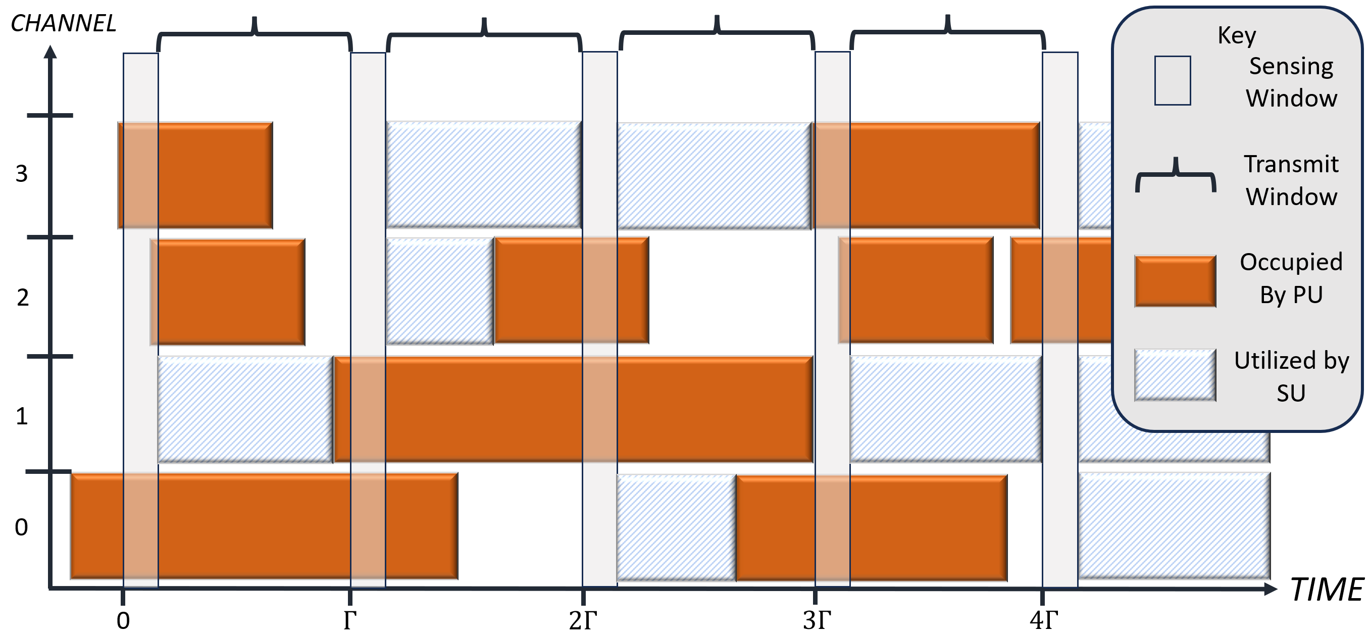
Figure 1. Timing diagram for PUs utilizing the channels. The SUs in a well-optimized SSRA-enabled CRN utilize the idle channels, i.e., the channels where the PU does not transmit.

Now, SU $n$ performs spectrum sensing, with a received signal on channel $\ell\in\mathcal{M}_{n}$, denoted as $z_{\ell}^{n}$ which follows one of the two following hypotheses:

(1) $$\mathcal{H}_{\ell}^{0}:~{}~{}z_{\ell}^{n}(i) =\nu_{\ell}^{n}(i),$$

$$\mathcal{H}_{\ell}^{1}:~{}~{}z_{\ell}^{n}(i) =\nu_{\ell}^{n}(i)+\xi_{\ell}^{n}(i).$$

$\mathcal{H}_{\ell}^{0}$ and $\mathcal{H}_{\ell}^{1}$ represent the idle and busy status of the PU on channel $k$, respectively. The noise present in the system is denoted as $\nu_{\ell}^{n}\sim\mathcal{CN}(0,\sigma^{2})$, and $\xi_{\ell}^{n}$ is the signal of the PU on channel ${\ell}$ received at SU $n$. All $\xi_{\ell}^{n}$'s are assumed to be independent and identically distributed zero-mean circularly symmetric complex Gaussian random variables with variance ($\sigma_{{\ell},n}^{\xi})^{2}$ on every channel $\ell$ at each SU $n$ (Fan and Jiang, 2010). Next, using the energy detection technique  (Hu et al., 2015), the test statistic of the signal energy of SU $n$ on channel ${\ell}$ is given as

(2) $$T_{\ell}^{n}=\frac{1}{\lfloor\varepsilon\tau/M\rfloor}\sum_{i=1}^{\lfloor\varepsilon\tau/M\rfloor}|z_{\ell}^{n}(i)|^{2};$$

which is compared to a threshold, $\psi_{\ell}^{n}$. If $T_{\ell}^{n}\leq\psi_{\ell}^{n}$, the SU $n$ determines the primary user to be idle on channel ${\ell}$; otherwise it is busy. We denote this choice as $x^{P}_{{\ell},n}\in\{0,1\}$, with $x^{P}_{{\ell},n}=0$ indicating that the FC has deemed the channel to be free (i.e., the SU believes that no PU is currently utilizing channel ${\ell}$) and $x^{P}_{{\ell},n}=1$ denoting the belief that ${\ell}$ is currently occupied. While the test statistics are themselves $\chi^{2}$ random variables, by employing the Central Limit Theorem (Atapattu et al., 2014), one can approximate the detection probability, $P^{\mathsf{de}}$, and false-alarm probability, $P^{\mathsf{fa}}$, as follows (Hu et al., 2015; Liang et al., 2008):

(3) $$P^{\mathsf{de}}(\psi_{{\ell}}^{n},\tau)=\mathsf{Pr}\left(T_{\ell}^{n}>\psi_{\ell}^{n}|\mathcal{H}_{\ell}^{1}\right)=\mathbb{Q}\left(\left(\frac{\psi_{\ell}^{n}}{\sigma^{2}}-\rho_{\ell}^{n}-1\right)\sqrt{\frac{\lfloor\varepsilon\tau/M\rfloor}{2\rho_{\ell}^{n}+1}}\right),$$

(4) $$\text{and}\,\,\,P^{\mathsf{fa}}(\psi_{\ell}^{n},\tau)=\mathsf{Pr}\left(T_{\ell}^{n}>\psi_{\ell}^{n}|\mathcal{H}_{\ell}^{0}\right)=\mathbb{Q}\left(\left(\frac{\psi_{\ell}^{n}}{\sigma^{2}}-1\right)\sqrt{\lfloor\varepsilon\tau/M\rfloor}\right).$$

The average SNR of the PU's signal received by SU $n$ on channel ${\ell}$ is denoted as $\rho_{\ell}^{n}=\left(\frac{\sigma_{{\ell},n}^{\xi}}{\sigma}\right)^{2}$ and $\footnotesize\mathbb{Q}(y)=\frac{1}{\sqrt{2\pi}}\int_{y}^{\infty}\exp\left(\frac{-u^{2}}{2}\right)du$ is the tail distribution of a standard normal variable (Liang et al., 2008).

Now, to achieve non-trivial spectrum sensing in practical CR networks, the detection probability should be at least 0.5 and the false-alarm probability at most 0.5. Thus, from (3) and (4), after several mathematical transformations, the constraints $P^{\mathsf{de}}\geq 0.5$ and $P^{\mathsf{fa}}\leq 0.5$ are equivalent to the following condition (Fan and Jiang, 2010):

(5) $$\sigma^{2}\leq\psi_{\ell}^{n}\leq\sigma^{2}(1+\rho_{\ell}^{n}),\forall{\ell}\in\mathcal{M}_{n}.$$

It is important to note that (1)-(5) are for the case of exclusively additive white Gaussian noise (AWGN). As we will present in subsequent sections, we utilize Rayleigh channel fading between the PUs and SUs, as well as between the SUs themselves. Accordingly, the equations do not account for instances of deep fading, which can be extremely detrimental to the energy detection scheme, as the heavily attenuated signal of the PU is no longer above the requisite detection SNR. Therefore, we modify $\mathcal{H}_{\ell}^{1}$ to include a Rayleigh-distributed channel gain, leaving

(6) $$\tilde{z}_{\ell}^{n}(i)=h_{\ell}^{P,n}(i)\xi_{\ell}^{n}(i)+\nu_{\ell}^{n}(i)$$

where $h_{\ell}^{P,n}$ is the gain on the PU's signal on channel ${\ell}$ as seen by SU $n$. However, as long as the coherence time $(t_{c})$ of the channels, which we assume to be fixed across all SUs and channels, is significantly lower than the length of the sensing window $(\tau)$, one can model the samples as having been taken from a non-fading AWGN channel. Then for any time $t>0$, $\mathcal{C}=\left\lceil{{\tau}/{t_{c}M}}\right\rceil$ is the total number of channel realizations seen per channel per sensing window. As $\mathcal{C}$ increases, the channel gain, $|h_{\ell}^{P,n}|^{2}$, is averaged out to $1$, meaning that the results in (2)-(5) hold true. We numerically demonstrate the impact of increasing $\mathcal{C}$ on $P^{\mathsf{de}}$ in Fig. 3.

2.2. Resource Allocation

In CR networks, the achievable throughput of the secondary network heavily depends on SUs' transmit power resource (Janatian et al., 2014) and on the transmission scheme they adopt. In keeping with common practice in modern wireless networks, we employ an orthogonal frequency division multiple access (OFDMA) scheme in the cognitive network (Tran and Pompili, 2018). Thus, four different cases of interest arise in the data collection phase:

Case 1: Channel $k$ is idle and is estimated to be idle. The probability that the SU correctly declares it not in use, given that a PU is not currently transmitting, is $\mathsf{Pr}(\mathcal{H}_{k}^{0})\left(1-P^{\mathsf{fa}}(\psi_{k}^{n},\tau)\right)$, where $\mathsf{Pr}(\mathcal{H}_{k}^{0})\geq 0$ is the idle probability of channel $k$ (Fan and Jiang, 2010). The achievable transmission rate of SU $n$ is thus

(7) $$R_{k,n}^{0}=\frac{B}{K}\log_{2}\left(1+\Upsilon^{0}_{k,n}\right),$$

where $\Upsilon^{0}_{k,n}$ is the received signal-to-interference-plus-noise ratio (SINR) of SU $n$ on channel $k$, which is defined as

(8) $$\Upsilon^{0}_{k,n}=\frac{x_{k}^{n}|h_{k}^{n,n}|^{2}p_{n}}{\sigma^{2}+\sum_{j\in\mathcal{N},j\neq n}\left(x_{k}^{j}|h^{j,n}_{k}|^{2}p_{j}\right)}.$$

Here $\sigma^{2}$ is the background noise variance, and the second term in the denominator is the interference among SUs on channel $k$. Furthermore, $|h^{\ell,m}_{k}|^{2}$ is the channel gain between the transmitter of SU $\ell$ and the receiver of SU $m$. $p_{\ell}$ is SU $\ell$'s transmit power, subject to $0\leq p_{\ell}\leq p_{\ell}^{\mathsf{max}}$, where $p_{\ell}^{\mathsf{max}}$ is SU $\ell$'s maximum power. Note that these transmit powers are not dependent on the channel; this stems from the fact that each SU has only one transmit antenna. Lastly, $x_{k}^{j}\in\{0,1\}$ indicates whether SU $j$ is transmitting on channel $k$ or not; if yes, $x_{k}^{j}=1$, and otherwise, $x_{k}^{j}=0$.

Case 2: Channel $k$ is actually busy, but it is estimated to be idle. The probability of estimating channel $k$ to be idle, while it is actually busy, is $\mathsf{Pr}(\mathcal{H}_{k}^{1})\left(1-P^{\mathsf{de}}(\psi_{k}^{n},\tau)\right)$, where $\mathsf{Pr}(\mathcal{H}_{k}^{1})=1-\mathsf{Pr}(\mathcal{H}_{k}^{0})$. The corresponding SU's signal serves as interference to the data transmission of PU, which goes against the fundamental purpose of a CRN setting. The achievable transmission rate of SU $n$ is given as

(9) $$R_{k,n}^{1}=\frac{B}{K}\log_{2}\left(1+\Upsilon^{1}_{k,n}\right),$$

where $\Upsilon^{1}_{k,n}$ is the received signal-to-noise ratio (SNR) of SU $n$ on channel $k$ which is given by

(10) $$\Upsilon^{1}_{k,n}=\frac{x_{k}^{n}|h^{n,n}_{k}|^{2}p_{n}}{\sigma^{2}+\sum_{j\in\mathcal{N},j\neq n}\left(x_{k}^{j}|h^{j,n}_{k}|^{2}p_{j}\right)+|h^{P,n}_{k}|^{2}p_{k}^{P}}.$$

Here, $p_{k}^{P}$ is the transmit power of the PU over channel $k$, and $h_{k}^{P,n}$ is the gain on channel $k$ between a PU and SU $n$.

Cases 3 (and 4): Channel $k$ is idle (or busy) and is estimated to be busy. No SUs will transmit on channel $k$, i.e., $x_{k}^{n}=0~{}\forall n\in\mathcal{N},\forall k\in\mathcal{K}$.

From (7) and (9), the average achievable rate of SU $n$ is given as

(11) $$R_{n}=\left(1-\frac{\tau}{\Gamma}\right)\sum_{k=1}^{K}(1-x^{P}_{k,n}) \Bigl{[}\mathsf{Pr}(\mathcal{H}_{k}^{0})\left(1-P^{\mathsf{fa}}(\psi_{k},\tau)\right)R_{k,n}^{0}$$

$$+\mathsf{Pr}(\mathcal{H}_{k}^{1})\left(1-Pr^{\mathsf{de}}(\psi_{k},\tau)\right)R_{k,n}^{1}\Bigr{]},$$

(12) $$\textrm{where we define,}\,\,\,x^{P}_{k,n}=\begin{cases}0,&T_{k}^{n}\leq\psi_{k}^{n}\\ 1,&\text{otherwise}\end{cases},~{}\forall k\in\mathcal{K},~{}\forall n\in\mathcal{N}$$

collected as $\bm{x}_{n}^{P}=\left[x_{1,n}^{P},x_{2,n}^{P},\dots,x_{K,n}^{P}\right]^{T}$. The multiplicative factor $(1-x^{P}_{k,n})$ prohibits the SU from transmitting in channel $k$ if it believes the PU to be transmitting there.

Without direct communication with the primary network, there is no way for the cognitive network to know with certainty whether or not a PU was transmitting on channel $k$ during a given sensing window. Thus, $x_{k,n}^{P}$ is the belief that a primary user is on channel $k$. However, with knowledge (or at least a conservative estimate) of the SNR of the PU (denoted by $\rho_{k}^{n}$), a good estimate for the presence of the PU is represented by $x_{k,n}^{P}$.

2.3. CRN Optimization Formulation

Having developed the average throughput at each SU, we can now formulate our optimization problem as below:

(13a) $$\underset{{\bm{X}},\bm{P}}{\operatorname*{\textrm{maximize}}} \sum_{n=1}^{N}R_{n}$$

(13b) s.t. $$x_{k}^{n}\in\{0,1\},~{}\forall n\in\mathcal{N},k\in\mathcal{K},$$

(13c) $$\sum_{k\in\mathcal{K}}x_{k}^{n}\leq 1,~{}\forall n\in\mathcal{N},$$

(13d) $$x^{P}_{k,n}\text{~{}as given in \eqref{eq:xpk},}$$

(13e) $$0<\tau<\Gamma,$$

(13f) $$\sigma^{2}\leq\psi_{k}^{n}\leq\sigma^{2}(1+\rho_{k}^{n}),~{}\forall k\in\mathcal{K},\forall n\in\mathcal{N}$$

(13g) $$P^{\mathsf{de}}(\psi_{k}^{n},\tau)\geq\mu,~{}\forall k\in\mathcal{K},\forall n\in\mathcal{N}$$

(13h) $$0<p_{n}\leq p_{n}^{\mathsf{max}},~{}\forall n\in\mathcal{N}.$$

Here, (13b) enforces the notion that any SU $n$ is either transmitting or idle on channel $k$, and (13c) prevents an SU from simultaneously accessing multiple channels for data transmission. Then, (13e) ensures the limited duration of spectrum sensing within the maximum time slot which in turn gives a feasible duration for data transmission. Next, (13f) aims to satisfy the constraints $P^{\mathsf{de}}\geq 0.5$ and $P^{\mathsf{fa}}\leq 0.5$. After that, (13g) enforces a lower bound on spectrum detection probability against a threshold $.5\leq\mu<1$. Finally, (13h) ensures that the transmit power of SU $n$ is limited to its max power.

The optimization problem above is potentially solvable only if (1) the SUs can communicate with the FC during each round of data transmission and (2) the FC issues power and channel-access directives thereafter. Thus, execution of the algorithm would remain centralized. Additionally, this would require SUs to exchange a very large amount of information among themselves in the form of channel gains, $h_{k}^{\ell,m},\ell\neq m$. As such, we will now revisit several terms in order to make the problem tractable by allowing for a solution which can be performed in a decentralized manner.

We assume that the SUs can obtain perfect knowledge of their respective channel gains, $h_{k}^{n,n}$. We collect our previously defined variables for SU transmission directive ($x_{k}^{n}$) as

(14) $${\bm{X}} =\begin{bmatrix}x_{1}^{1}\cdots x_{K}^{1}\\ \vdots\ddots\vdots\\ x_{1}^{N}\cdots x_{K}^{N}\end{bmatrix}_{N\times K,}=\left[\bm{x}^{1},\bm{x}^{2},\dots,\bm{x}^{N}\right]^{T}$$

SU $n$ has local knowledge of the $n^{\text{th}}$ row of $\bm{X}$, but no data is exchanged directly between any two SUs.

Next we consider the term, $\sum_{n}^{N}R_{n}$, which is not calculable since the gains, $h_{k}^{\ell,m},\ell\neq m$, are not known. Instead, our assumption is that the SUs create an estimate of their SNR to estimate (11). During the transmission window, the SUs estimate the channel they are transmitting on, $\widehat{h}_{k}^{n,n}$. Next, they sample the channel at predetermined times to obtain an estimate of the sum of the interference and the noise, $(\widehat{\sigma}_{k}^{n})^{2}$. These times need to be set in a way such that no two SUs sample channel $k$ at the same time so that the interference of other SUs is accounted for in the estimate of the interference plus the noise. With knowledge of the transmit power, $p_{n}$, utilized, the SNR can be estimated as $\widehat{\Upsilon}_{k,n}=\frac{\left|\widehat{h}_{k}^{n,n}\right|^{2}p_{n}}{\left(\widehat{\sigma}_{k}^{n}\right)^{2}}$, yielding an empirical datarate of

(15) $$\widehat{R}_{n}=\sum_{k\in\mathcal{M}_{n}}(1-x_{k,n}^{P})x_{k}^{n}\log_{2}\left(1+\widehat{\Upsilon}_{k,n}\right)$$

While we write this as a sum across all channels for completeness, a given SU only needs to consider the channel on which it is transmitting. The goal of the problem is to therefore maximize the estimated sum transmission rate of the network, denoted by $\widehat{R}=\sum_{n=1}^{N}\widehat{R}_{n}$.

3. Multi-Agent Hybrid SAC Formulation

Having outlined the problem, we now introduce the mechanism by which we intend to solve it. Due to the non-convex and multi-agent nature of the problem, we turn to multi-agent deep reinforcement learning (MARL), a field which has shown promise in solving such problems (Feng et al., 2020). In particular, we develop a novel multi-agent implementation of hybrid Soft Actor-Critic (Delalleau et al., 2019) (HSAC), which we call ``MHSAC''. We begin by providing a formal definition of general MARL problems. Next, we present the equations governing the actor and critic networks for the HSAC framework, then work them into a multi-agent setting.

3.1. Overview of Dec-POMDP MARL

An intuitive way to optimize the network while ensuring no inter-agent communication is to train the respective actor and critic networks for each agent solely based on local information. This does not, however, lead to a convergent network since the reward of one SU is dependent on the actions taken by the others. In the process of greedily maximizing their rewards without any communication of results, the SUs would then be training in a non-stationary environment, which a (non-MARL) DRL agent may not be capable of solving. Therefore, we consider the centralized training, decentralized execution (CTDE) paradigm of training a multi-agent system.

In CTDE, agents periodically communicate their actions, observations, and rewards to the fusion center but not directly with each other. With observations, actions, and rewards from all SUS, the FC can then train an aggregated critic model which enables convergence in a multi-agent setting. We therefore model our cognitive radio network as a decentralized partially observable Markov decision process (Dec-POMDP) $G=\left\langle\bm{S},\bm{A},\bm{P},r,\bm{\Omega},N,\gamma\right\rangle$, where $\bm{S}$ is the global state; $\bm{\Omega}$ is the full observation space; $\bm{A}$ is the action space; $N$ is the total number of agents; and $\gamma$ is a discounting factor. At each time-step, SU $n$ obtains observation $\bm{o}^{n}\in\bm{\Omega}$ and selects action $\bm{a}^{n}\in\bm{A}_{n}$. The individual actions of the SUs are collected into $\bm{a}\in\bm{A}$, which represents the joint action of the system. Following these actions being performed, the system obtains a joint reward, $r(\bm{s},\bm{a})$ and transitions to its next state following $\bm{P}(\bm{s}^{\prime}|\bm{s},\bm{a})$, which is the probability of transitioning to state $\bm{s}^{\prime}$ given that the system is currently in state $\bm{s}$ and has taken action $\bm{a}$. Each agent learns a policy $\pi^{n}(\bm{a}^{n}|\bm{o}^{n})$ which seeks to output the optimal action given an observation of the environment. The joint policy can thus be expressed as $\bm{\pi}=\left\langle\pi^{1},\pi^{2},\dots,\pi^{N}\right\rangle$, which is used to calculate the joint Q-function at the critic:

(16) $$Q_{\pi}^{tot}(\bm{o},\bm{a})=\mathbb{E}_{\bm{s},\bm{a}}\left[\sum_{t=0}^{\infty}\gamma^{t}r(\bm{s}_{t},\bm{a}_{t})|\bm{s}_{0}=\bm{s},\bm{a}_{0}=\bm{a},\bm{\pi}\right].$$

This Q-function is the mechanism by which the critic assesses the efficacy of and induces updates to the policy, $\bm{\pi}$, during training.

3.2. Actor-Critic Model Architecture

In a real-world CRN setting, taking a greater number of samples to converge means greater likelihood of colliding with the PUs during training. It is therefore imperative that the DRL framework be sample-efficient, something which the Soft Actor-Critic model (SAC) architecture (Haarnoja et al., 2019) is noted for. However, while the $p_{n}$s are continuous variables and thus fit directly into a basic SAC framework, $\bm{X}$ is a collection of discrete decisions on whether or not a channel should be accessed. Accordingly, we utilize the hybrid discrete/continuous Soft Actor-Critic model (HSAC) proposed in (Delalleau et al., 2019); a diagram of this architecture is shown in Fig. 1. In this subsection, we present HSAC in a general setting, and in the next we develop a multi-agent application thereof. The goal of (Hua et al., 2022) was to develop hybrid SAC in an MARL setting. However, their agents share their observations, actions, and rewards directly with one another, with each agent maintaining its own ``independent global critic network''. This MARL methodology becomes intractable as the network grows in size due to the amount of information which must be shared between the SUs.

The continuous portion of the model acts identically to SAC, with another separate linear activation layer yielding one of $\bm{D}$ discrete outputs in parallel to the continuous portion of the network. These $\bm{D}$ outputs are fed through a categorical distribution as logits; the resultant discrete distribution, $\pi_{d}$, is then sampled to determine which channel to transmit on (or to remain idle). In our work, we do not pass the discrete actions as inputs into the critic network since the authors of (Delalleau et al., 2019) note that it makes little discernible impact on model performance.

A major difference between HSAC and standard SAC is in how the entropy is calculated. The joint (Shannon) entropy for a user, $H(\pi|\bm{s})$, of the discrete and continuous variables is given as

(17) $$H(\pi|\bm{s})= ~{}\alpha_{d}H\left(\pi_{d}(\bm{a}_{d}|\bm{s})\right)+\alpha_{c}\sum_{\bm{a}_{d}\in\bm{A}}\pi_{d}(\bm{a}_{d}|\bm{s})\mathcal{H}\left(\pi_{c}(\bm{a}_{c}|\bm{s},\bm{a}_{d})\right)$$

where for some discrete random variable $Y$ which can take on values in $\mathcal{Y}$, $H(Y)\triangleq-\sum_{y\in\mathcal{Y}}\mathsf{Pr}(y)\log\mathsf{Pr}(y)$, with $\mathsf{Pr}(y)$ being the probability measure of event $y$, and $\mathcal{H}(\pi(\cdot))=-\log(\pi(\cdot))$. Additionally, (Delalleau et al., 2019) notes that it is often the case that the continuous actions are independent of the discrete actions and can therefore be modeled without conditioning. Thus, (17) can be reduced to

(18) $$\begin{aligned} H(\pi|\bm{s})=\sum_{\bm{a}_{d}\in\bm{A}}\pi_{d}(\bm{a}_{d}|\bm{s})\Big{[}\alpha_{d}\mathcal{H}\left(\pi_{d}(\bm{a}_{d}|\bm{s})\right)+\alpha_{c}\mathcal{H}\left(\pi_{c}(\bm{a}_{c}|\bm{s})\right)\Big{]}\end{aligned},$$

where $\alpha_{d}$ and $\alpha_{c}$ are indepndently tunable temperatures for the discrete and continuous entropies, respectively.

Next, we address the output of the Q-network. Unlike traditional SAC, the output of the critic network in HSAC is represented by $\bm{D}$ outputs, $\bm{q}=[q_{1},q_{2},\dots,q_{\bm{D}}]^{T}$, each corresponding to the value which could be obtained by taking action $\bm{a}_{d}$. Thus, $Q$ is given by $Q=q_{a_{d}}$, where $a_{d}$ is the discrete action taken.

3.3. Multi-Agent HSAC

Here, we develop the use of HSAC in a multi-agent setting, which we refer to henceforth as ``MHSAC''. Across the network, each agent maintains the following networks: policy (actor); two value networks (critic), $Q_{i}^{n},i=1,2$; and two target value functions, $Q_{j}^{n,targ},j=1,2$. We utilize two Q-networks to increase the stability of the training process. The output of each local Q-network is an estimate of the reward received by that agent. Let the Q-networks be parameterized by $\phi_{n}$, where $Q_{\phi_{n}}^{n}$ now represents the deep learning-based approximation to the true Q-function of agent $n$. The total value as seen across the network is then some aggregation of these Q-networks, $Q^{tot}$, created so as to preserve monotonic mixing of the Q-values across the network (Rashid et al., 2018), in other words, $\frac{\partial Q^{tot}}{\partial Q^{n}}\geq 0,\forall n\in\mathcal{N}$. This condition enforces consistency between the joint and decentralized action-value functions:

(19) $$\operatorname*{argmax}_{\bm{a}}Q^{tot}=\left(\operatorname*{argmax}_{\bm{a}^{1}}Q^{1},\dots,\operatorname*{argmax}_{\bm{a}^{N}}Q^{N}\right).$$

We employ the mixing network from the QMIX algorithm (Rashid et al., 2018), an RNN-based network which uses all $Q^{n}$ as inputs to a linear layer and all observations $\bm{o}$ from across the network as inputs into hidden layers. This hypernetwork then outputs $Q^{tot}$:

(20) $$Q^{tot}=f_{qmix}(Q^{1},\dots,Q^{N};\bm{o}).$$

This establishes the value function for the whole network. Similar to the approach in (Pu et al., 2021), we can now write the loss-functions which will be used to update the networks. We treat the agents as homogeneous in the sense that they maintain the same action- and observation-spaces. The network parameters, $\phi$, are trained end-to-end to minimize the critic loss, $\mathcal{L}(\phi)$

(21) $$\mathcal{L}(\phi)=\frac{1}{2}\sum_{i=1,2}\mathbb{E}_{\mathcal{D}}\left[\left(r_{t}+\gamma\min_{j\in\{1,2\}}Q_{\phi_{j}^{\prime}}^{targ}-Q_{\phi_{i}}^{tot}\right)\right]$$

where $\mathcal{D}$ is a replay buffer storing the observations, actions, rewards, and next observations. $Q_{\phi_{1}}^{tot}$ is the output of the mixing network for $\{Q_{1}^{1},\dots,Q_{1}^{N}\}$; $Q_{\phi_{2}}^{tot}$ stems from the $Q_{2}^{n}$ networks.

Next, the target value function is given as

(22) $$Q_{\phi_{j}^{\prime}}^{targ} =\mathbb{E}_{\bm{\pi}}\left[Q_{\phi_{j}^{\prime}}^{tot}(\bm{s}_{t+1},\bm{o}_{t+1},\bm{a}_{t+1})+H(\pi(\bm{a}_{t+1}|\bm{o}_{t+1}))\right]$$

$$=\sum_{n=1}^{N}(\pi_{d}^{n}(\bm{a}_{t+1}|\bm{o}_{t+1}))^{T}\bm{q}_{\phi_{j}^{\prime}}^{n}+H^{n}(\pi^{n}(\bm{a}_{t+1}^{n}|\bm{o}_{t+1}^{n})).$$

Here and elsewhere, we use $\phi$ and $\phi^{\prime}$ to differentiate between the parameters of the evaluation and target Q-networks, respectively.

Next, let the policy network be parameterized by $\theta$. The goal of the actors is then to minimize the loss $\mathcal{L}(\theta)$ as

(23) $$\mathcal{L}(\theta) =\mathbb{E}_{\mathcal{D}}\left[H(\bm{\pi}(\bm{a}_{t}|\bm{o}_{t}))-Q_{\phi}^{tot}(\bm{s}_{t},\bm{o}_{t},\bm{a}_{t})\right]$$

$$={E}_{\mathcal{D}}\left[\sum_{i=1}^{N}H(\pi^{n}(\bm{a}_{t}^{n}|\bm{o}_{t}^{n}))-\min_{j=1,2}Q_{\phi_{j}}^{n}(\bm{o}_{t}^{n}\bm{a}_{t}^{n})\right].$$

To automatically tune $\alpha_{d}$ and $\alpha_{c}$ during the training process, two more networks are needed, subject to the following loss functions:

$$\mathcal{L}(\alpha_{d}) =\mathbb{E}_{\bm{a}_{t}\sim\bm{\pi_{t}}}\left[-\alpha_{d}\log\left(\bm{\pi}_{t}(\bm{a}_{d,t}|\bm{o}_{t})\right)-\alpha_{d}\bar{\mathcal{H}}_{d}\right]$$

$$\textrm{and}\,\,\,\,\mathcal{L}(\alpha_{c}) =\mathbb{E}_{\bm{a}_{t}\sim\bm{\pi_{t}}}\left[-\alpha_{c}\log\left(\bm{\pi}_{t}(\bm{c}_{d,t}|\bm{o}_{t})\right)-\alpha_{c}\bar{\mathcal{H}}_{c}\right]$$

where $\bar{\mathcal{H}}$ is the target entropy.

4. MHSAC-Based SSRA Methodology

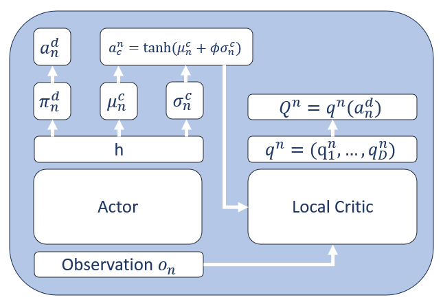
(a) Hybrid SAC model for a single agent.

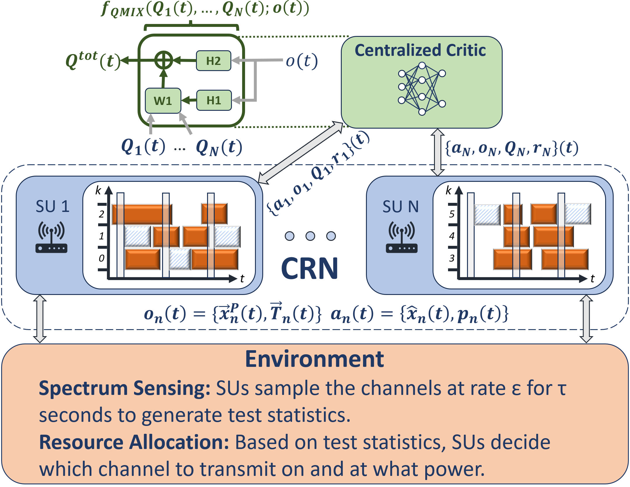
(b) Centralized training-decentralized execution setting for CRN.

Figure 2. Architectures for a single agent and the overall network. Here, $\bm{o}_{n}$ comprises test statistics and channel occupancy beliefs, $\bm{a}_{n}^{d}$ is the decision of which channel to utilize, and $\bm{a}_{c}^{n}$ is the transmit power. The expected reward of choosing discrete action $\bm{a}_{i}^{d}$ is $q_{i}^{n}$. The trainable mean and variance of the reparameterization trick employed by SAC are $\mu_{n}^{c}$ and $\sigma_{n}^{c}$, respectively.

Having developed the generic MHSAC architecture, we now present the observation space, the action space, and the reward for our SSRA optimization problem. We then outline the metrics by which we will characterize the performance of our algorithm in the network. We call this algorithm ``HySSRA''.

4.1. Observation

The observation of each SU, $\bm{o}^{n}_{t}$, in the SSRA scheme consists of two parts. First is the belief on the presence of the primary users on the channel, $\bm{o}_{t}^{n,x}$, calculated by comparing the test statistics against the thresholds, as in (12). Additionally, the test statistics, $\bm{o}_{t}^{n,T}$, are provided as inputs. Thus, our SAC model receives inputs $\bm{o}_{t}^{n}=\{\bm{o}_{t}^{n,x},\bm{o}_{t}^{n,T}\}$, given as $\bm{o}_{t}^{n,x}=\bm{x}_{n}^{P}$ and $\bm{o}_{t}^{n,T}=\left[T_{1}^{n}(t),\dots,T_{K}^{n}(t)\right]$, where $\bm{x}_{n}^{P}$ and $T_{k}^{n}$ are as given in (14) and (2), respectively.

4.2. Action

Based on its observation, the actor model at each SU makes decisions on channel access directives, $\bm{x}_{t}^{n}$, and transmit power, $p_{n}(t)$. Each SU decides to access at most one channel $k\in\mathcal{K}$, or else it remains idle. Thus, the action at time $t$ is given by $\mathbf{a}_{t}^{n}=\{\mathbf{a}_{t}^{n,x},\mathbf{a}_{t}^{n,p}\}$, with each member of the set defined as $\mathbf{a}_{t}^{n,x}=\widehat{{x}}^{n}(t)$ and $\mathbf{a}_{t}^{n,p}=p_{n}(t)$, subject to the previously outlined constraints. Lastly, note that we use $\widehat{x}^{n}(t)$ instead of $\bm{x}^{n}(t)$ directly in the action-space so as to conform to the hybrid continuous/discrete SAC model previously developed. Let $\widehat{x}^{n}(t)\in\{1,2,\dots,K+1\}$. Here, $\widehat{x}^{n}=k\leq K$ indicates the action of SU $n$ transmitting on channel $k$, and $\widehat{x}^{n}=K+1$ corresponds to the choice to remain idle.

4.3. Reward

By executing the action $\bm{a}_{t}=\langle\bm{a}_{t}^{1},\dots,\bm{a}_{t}^{N}\rangle$ under the state $\bm{s}_{t}$, the SUs can obtain their empirical datarate, $\widehat{R}_{n}$, as defined in (15). We introduce two penalty terms which will detract from each agent's reward upon violation. First, we the penalize SUs for electing to transmit on a channel which is deemed occupied by indexing the occupancy belief vector with the channel access decision:

(24) $$\Delta_{occ}^{n}=\lambda_{occ}^{n}\times\begin{cases}\bm{x}_{n}^{P}[\widehat{x}^{n}],&\widehat{x}^{n}\leq K\\ 0,&\text{otherwise}\end{cases}.$$

More clearly, if an SU determines the PU to be on a channel but still decides to transmit on it, the reward will incur a penalty of $\lambda_{occ}^{n}>0$. This helps to reduce collisions between the secondary users and the primary network throughout the training and inference processes.

Next, we add a penalty which helps to mitigate interference both from the SUs to one another and from the SUs to the primary network, $\Delta_{rate}^{n}$. Let $\zeta>0$ be a target rate, below which the secondary user is very likely to be interfering with members of the CRN or the primary network. Then

(25) $$\Delta_{rate}^{n}=||\bm{x}^{n}||^{2}\times\begin{cases}\lambda_{rate}^{n},&\widehat{R}_{n}<\zeta\\ 0,&\text{otherwise}\end{cases},$$

where $\lambda_{rate}^{n}>0$ is a weighting factor. $||\bm{x}^{n}||^{2}$ is the choice of the secondary user to transmit or not; it is equal to 0 when the SU doesn't transmit and 1 when it does.

We then set the reward at SU $n$ as

(26) $$r^{n}(\bm{o}_{t}^{n},\bm{a}_{t}^{n})=-\Delta_{occ}^{n}(t)+\begin{cases}\widehat{R}_{n}(t),&\widehat{R}_{n}(t)\geq\zeta\\ -\Delta_{rate}^{n}(t),&\text{otherwise}\end{cases}$$

with the fusion center generating an overall reward across the network as the sum of the SUs' rewards, $r_{t}=r(\bm{s}_{t},\bm{a}_{t})=\sum_{i=1}^{N}r^{i}(\bm{o}_{t}^{i},\bm{a}_{t}^{i})$. It is assumed that the SUs always have information to send.

4.4. Metrics of Interest

While the usual goal in any RL-based problem is only to maximize the reward, there are several metrics which, we believe, need to be considered as well for assessing the efficacy of the model:

4.4.1. Idle Channel Utilization Rate

If a channel is idle, it is expected that the SUs detect this, and upon convergence of the DRL scheme, transmit on that channel. We quantify this with the following usage rate of idle channels. Define this rate as

(27) $$\omega^{i}={\sum_{k\in\mathcal{K}}\left((1-I_{k})\mathbbm{1}_{x(k)}\right)}/{\min\{K-I,N\}}\geq 0$$

where $\mathbbm{1}_{x(k)}=1$ if any secondary user opts to transmit on channel $k$ and equals $0$ otherwise. $I=\sum_{k\in\mathcal{K}}I_{k}$ is the number of channels actually in use by the PUs, where $I_{k}=1$ if the channel is in use by the PU and $0$ otherwise. We emphasize that the CRN does not know $I$. It is only used to demonstrate the efficacy of our algorithm under varying settings in subsequent sections. It should be the case that $\omega_{i}\approx 1$ upon convergence when $N\geq K$.

4.4.2. Occupied Channel Utilization Rate

Similar to the above, we are also interested in the rate at which the SUs use channels which are being used by the PUs. The rate of utilizing occupied channels is $\omega^{o}=\sum_{k\in\mathcal{K}}(\mathbbm{1}_{x(k)}I_{k})/I$. As the algorithm converges, $\omega^{o}\rightarrow 0$ shows that the SUs are not interfering with the primary network.

4.4.3. SU-SU Collisions

Another important metric of interest is the rate at which secondary users collide with one another. It is expected that secondary users do not opt to transmit on the same channel at the same time when the algorithm has converged. The collisions are $\omega^{c}=\sum_{k\in\mathcal{K}}\omega^{c}(k)$, where $\omega^{c}(k)=\sum_{n\in\mathcal{N}}x_{k}^{n}$ if $\geq 2$ SUs use channel $k$ simultaneously and is $0$ otherwise.

5. Experimental Results

In this section, we first demonstrate the necessity of observing multiple channel realizations on detection probability. Next, we show the efficacy of our proposed algorithm. These experiments are run with the parameters outlined in Tables 1 and 2 and the values below. We set the threshold $\psi_{k}^{n},~{}\forall n\in\mathcal{N},~{}\forall k\in\mathcal{K}$ as $\psi_{k}^{n}=({\sigma^{2}+\sigma^{2}(1+\rho_{k}^{n})})/{2}$, which was experimentally observed to be effective in achieving the metrics described in Sec. 4.4.2. We set $\tau$ and $\epsilon$ such that each channel sees $\mathcal{C}=5$ realizations, with $20$ samples taken per realization. Under this setup, we note that channels are correctly identified as being either idle or occupied approximately $94\%$ of the time.

The PUs utilize BPSK to transmit their symbols. Constellations for which symbols are not equidistant from the origin (e.g., QAM) may require other considerations when setting $\psi_{k}^{n}$, such as, for example, basing the threshold off of the symbols which are sent with the least power. We draw the probability of channel $k$ going from idle to occupied, $\mathsf{Pr}(i\rightarrow o)$, uniformly at random as $\mathcal{U}(.2,.5)$, with $\mathsf{Pr}(i\rightarrow o)$ on $k$ being drawn independently of $\mathsf{Pr}(i\rightarrow o)$ for $k^{\prime}\neq k$. The $\mathsf{Pr}(o\rightarrow o)$ probabilities are generated similarly.

An exponential weighted average with a factor of 0.2 serves as an overlay in plots. Each point on all subsequent graphs (except Fig. 3(a)) is the average of the previous 100 steps taken in the environment.

Table 1. Environment Parameters

Parameter	Value	Units
$K,~{}N$	$12,~{}6$	N/A
$\varepsilon$	$1E4$	samp/sec
$t_{c}$, $\tau$, $\Gamma$	$2E-3$, $M\times 1E-2$, $1$	s
$\sigma^{2}$, $p_{n}^{\mathsf{max}}$, $p_{k}^{P}$	$5E-3$, $5E-3$, $1$	Watts
$\Delta_{occ}^{n}$, $\Delta_{rate}^{n}$	$10,~{}2.5$	N/A
$\zeta$	$0.1\times\log_{2}\left(1+\frac{p_{n}^{\mathsf{max}}}{2\sigma^{2}}\right)$	N/A
$\mathsf{Pr}(i\rightarrow o)$, $\mathsf{Pr}(o\rightarrow o)$	$\sim\mathcal{U}(.2,.5)$, $\sim\mathcal{U}(.6,.9)$	N/A

Table 2. DRL Network Parameters

Parameter	Value
Episode length, Total timesteps, Mini-batch	$3E3$, $6E4$, $64$
Policy frequency, $\gamma$, $|\mathcal{D}|$	$10$, $0.4$, $3E4$
$\widebar{\mathcal{H}}_{c}$, $\widebar{\mathcal{H}}_{d}$	$0.0$, $0.01\times M$
Actor, Critic hidden layers	$256\rightarrow 128\rightarrow 64$
Actor, Critic learning rates	$1E-4,~{}1E-3$
Activations	ELU

5.1. Impact of Channel Realizations

Figure 3(a) demonstrates the impact of the number of channel realizations seen $\mathcal{C}$ on the probability of detecting a primary user on a given channel. We set the PU's transmit and the noise power both to $1$ mW. The sensing window is set as $\tau=1,2,\dots,25$. We observe $P^{\mathsf{de}}$ for the four possible combinations of $\varepsilon=10,20$ and $t_{c}=0.5,1$. The cases labeled ``$A(\varepsilon)$'' are the probability of detection for a non-fading channel sampled at rate $\epsilon$, calculated using (3). At each $\tau=1,2,\dots,25$, the points on the ``$R(\varepsilon,~{}t_{c})$'' curves represent the average of 1000 instances of sensing an occupied channel. It is evident that multiple channel realizations must be seen for the spectrum sensing performance of the fading case to be comparable that of an AWGN channel. The $R(\cdot,0.5)$ curves experience twice as many channel realizations per sensing window than the $R(\cdot,1)$ curves and as such approach the corresponding AWGN cases at a much smaller $\tau$. For fixed $t_{c}$, the number of samples taken per channel realization has a proportionally smaller impact, indicating that the number of channel realizations are of greater importance.

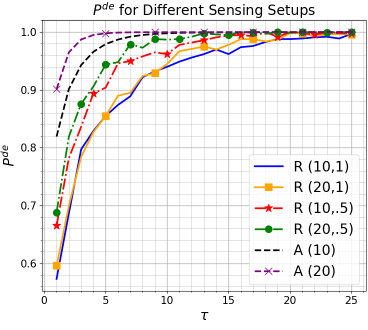
(a) Plots labeled ``$R~{}(\varepsilon,t_{c})$" are Rayleigh channels sampled at rate $\varepsilon$ with coherence time $t_{c}$; each point is the average of 1000 sensing decisions. ``$A(\varepsilon)$" are AWGN channels, calculated numerically via (3).

(b) The usage rate of occupied channels, when $N=2$ users sense $K=M=4$ channels. This shows how sensing multiple channel realizations can help alleviate the problem of a PU's being in a bad fade at an SU.

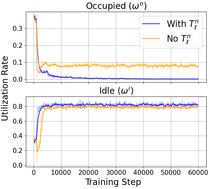
(c) Rate of usage for occupied and idle channels for observation spaces with and without test statistics. For only a small increase in overall usage rate in idle channels, greatly increasing the collision with PUs.

Figure 3. Spectrum sensing-related graphs. Fig. (a) and (b) capture the impact of the number of channel realizations, $\mathcal{C}$, seen over the sensing window on model convergence. Fig. (c) demonstrates the need for test statistics in the observation space.

In Fig. 3(b), we experimentally demonstrate the impact of the number of channel realizations seen on the rate of utilizing occupied channels. We set $K=M=4$ and $N=2$, with $\tau=0.016$ seconds. Thus, each channel is sampled 40 times. For the blue line, $t_{c}=4E-3$, so each channel is only sensed over one realization, and for the orange, $t_{c}=1E-3$, yielding $\mathcal{C}=4$. Considerably more interference with the primary network is observed in the case of smaller $\mathcal{C}$.

5.2. Importance of Test Statistics in Observations

Fig. 3(c) demonstrates the importance of including the test statistics for each channel, $T_{\ell}^{n}$, in the inputs to each agent's models. We set $P=K=12$ and $N=6$. Plots labeled ``No $T_{\ell}^{n}$'' have $\bm{o}_{t}^{n,T}$ removed from the observation space of each agent; other plots feature the full observation space. While both cases realized similar long-term rewards, it is very apparent that the model run without test statistics interferes with the primary network significantly more often than the model run with our proposed action space. To minimize interference with the PUs, test statistics should be included in the observation space, a consideration not taken in the DSA literature.

5.3. Varying Number of SUs and PUs' SNRs

Fig. 4 explores the impact of network parameters on the convergence of our algorithm. In each case, there are $K=12$ channels, with $N=6$ SUs for the middle plots. For Figs. 4(a) and 4(b), each SU senses $M=\lceil K/N\rceil+1$ channels; Fig. 4(c) has each SU sense $1$ channel. The graphs corroborate the intuition behind the metrics laid out in Sec. 4.4.2. Lastly, note that the SUs reach slightly below $p_{n}^{\mathsf{max}}$, which we believe this to be the result of the $\tanh$ squashing function used in SAC saturating (see Fig. 2(a) and (Haarnoja et al., 2019)). However, the difference in reward is negligible between achieving $p_{n}^{\mathsf{max}}$ and the the power to which HySSRA converges. Meanwhile, the power ramp-up helps mitigate interference with the PUs early in the training process. The four power lines on Fig. 4(c) which do not tend to $p^{n}_{max}$ are the SUs whose models converged to never transmit, illustrating that HySSRA does not ensure fairness.

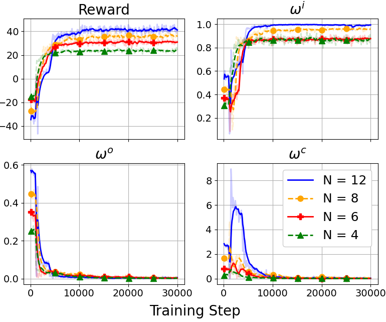
(a) Varying number of secondary users. In all cases, $\omega^{o}$ saturates to $0$, as expected. Additionally, when $N=K$, we see that $\omega^{i}$ saturates to $1$, indicating full usage of empty channels. Cases with higher $N$ experience more SU-SU collisions earlier in training, however $\omega^{c}$ always saturates to $0$.

(b) Plots for different PU transmit power, $p^{P}$ with $N=6$ SUs. As $p^{P}$ decreases, we can see a noticeable increase in the rate of collisions with the primary network. However, the usage rate of idle channels decreases, indicating a more conservative nature of the SUs in accessing spectrum.

(c) $K=12$ channel network with $N=16$ SUs sensing 1 channel each. The variable power allows the CRN to interfere less with the PUs before the model has converged. This also demonstrates the ability of our proposed HySSRA algorithm to converge in over-subscribed networks.

Figure 4. Metrics of interest for various network configurations. $\omega^{i}$ is the usage rate of idle channels, $\omega^{o}$ is the usage rate of channels occupied by PUs, and $\omega^{c}$ is the rate of collisions between secondary users. .

5.4. Model Performance Versus Baseline

Fig. 5 demonstrates the effectiveness of HySSRA relative to a current state-of-the-art DSA algorithm, CoMARL-DSA (Tan et al., 2022). Whereas we fix the channels a given SU senses beforehand to learn the allocation, CoMARL-DSA determines which channels a given SU should sense. The overall goal of both algorithms, however, is having a CRN efficiently use idle spectrum. For CoMARL, we train for 600 epochs. Each epoch is 10 episodes at 10 steps per episode, with 10 training steps taken per epoch on size 64 mini-batches. This maintains consistency with the total number of steps taken in the environment and the training frequency between algorithms. Our energy detection setup is deployed for both algorithms based on Table 1. The same Markov transition chain is used in all experiments. The transmit power for CoMARL-DSA is fixed to $p_{n}^{\mathsf{max}}$.

Fig. 5 shows the corresponding results where we observe that our proposed HySSRA outperforms CoMARL-DSA on all metrics considered. It enjoys faster convergence, justifying the claim that HySSRA is relatively sample-efficient. This is critical in CRN settings because any interference with the primary user is an infringement on their priority rights to the spectrum; a quicker convergence can alleviate these concerns. In the cases which feature 10 channel realizations, we set $\tau=40~{}ms$ and leave everything else constant; this yields correct identification of the channel as idle or occupied at a rate of around $98\%$.

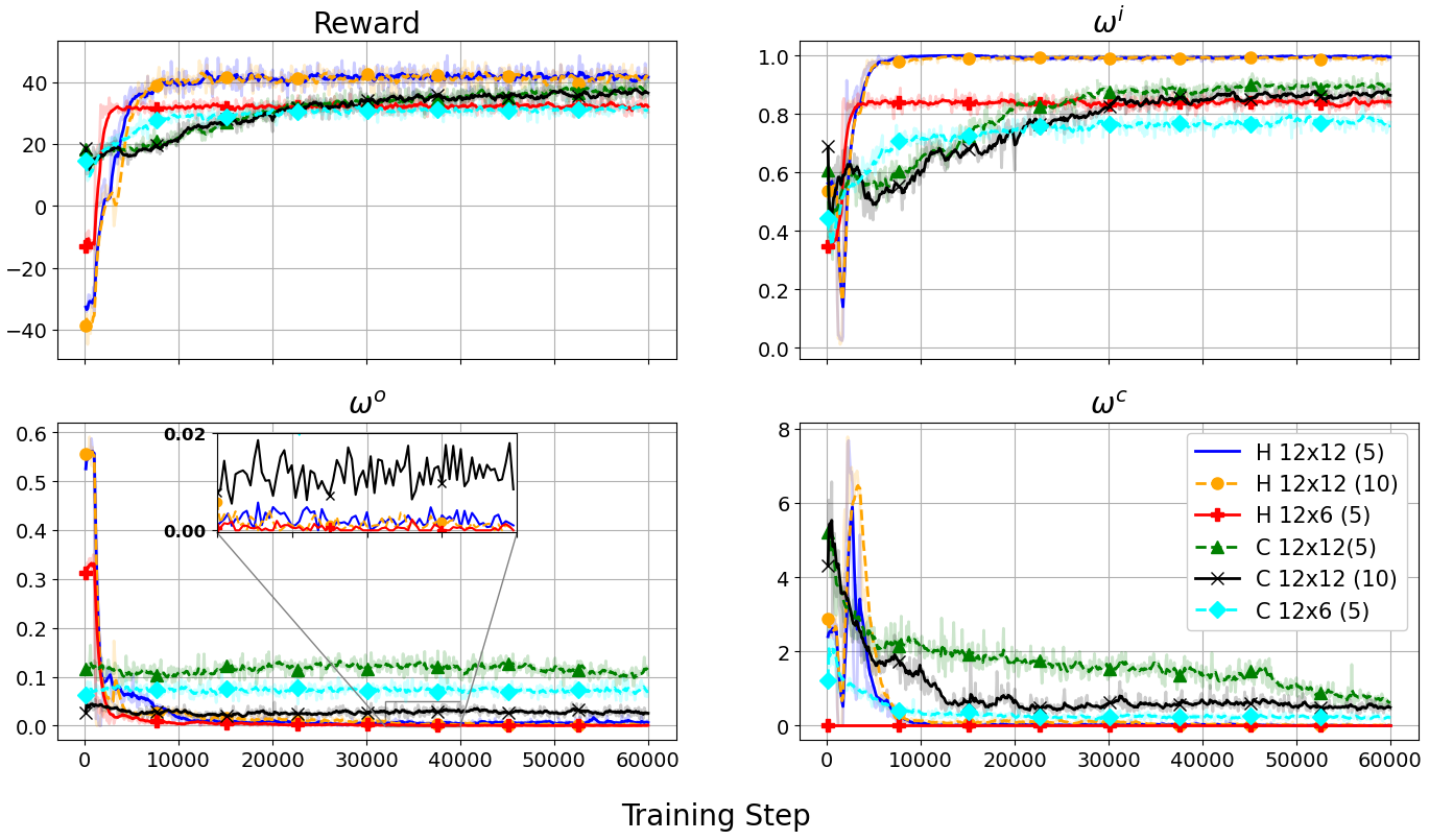
Figure 5. Comparison of HySSRA against CoMARL-DSA, a state-of-the-art DSA algorithm. The convention for the legend is ``H (C) = HySSRA (CoMARL-DSA) $K\times N$ ($\mathcal{C}$), where $\mathcal{C}$ is the number of channel realizations seen per channel. HySSRA demonstrates superior performance on all metrics. As $\mathcal{C}$ increases, the performance of CoMARL-DSA becomes more comparable to HySSRA.

6. Conclusions

In this work, we have proposed a highly-effective spectrum sensing/resource allocation algorithm, HySSRA, for opportunistic spectrum access in cognitive radio networks. To do this, we developed a novel multi-agent MARL framework, HSAC, which is capable of outputting both continuous and discrete actions. Our results showed considerable sample efficiency coupled with improvement over a state-of-the-art algorithm with regards to efficient use of idle channels and consistent non-use of occupied channels.

References

- (1)
- Atapattu et al. (2014) Saman Atapattu, Chintha Tellambura, and Hai Jiang. 2014. Energy detection for spectrum sensing in Cognitive Radio. Springer New York.
- Chang et al. (2019) Hao-Hsuan Chang, Hao Song, Yang Yi, Jianzhong Zhang, Haibo He, and Lingjia Liu. 2019. Distributive Dynamic Spectrum Access Through Deep Reinforcement Learning: A Reservoir Computing-Based Approach. IEEE Internet of Things Journal 6, 2 (2019), 1938–1948. https://doi.org/10.1109/JIOT.2018.2872441
- Chen et al. (2016) Huifang Chen et al. 2016. Joint spectrum sensing and resource allocation scheme in cognitive radio networks with spectrum sensing data falsification attack. IEEE Transactions on Vehicular Technology 65, 11 (2016), 9181–9191.
- Chen et al. (2020) Xiping Chen, Xianzhong Xie, Zhaoyuan Shi, and Zishen Fan. 2020. Dynamic Spectrum Access Scheme of Joint Power Control in Underlay Mode Based on Deep Reinforcement Learning. In 2020 IEEE/CIC International Conference on Communications in China (ICCC). 536–541.
- Delalleau et al. (2019) Olivier Delalleau, Maxim Peter, Eloi Alonso, and Adrien Logut. 2019. Discrete and Continuous Action Representation for Practical RL in Video Games. arXiv:1912.11077 [cs.LG]
- Devroye et al. (2008) Natasha Devroye, Mai Vu, and Vahid Tarokh. 2008. Cognitive radio networks. IEEE Signal Processing Magazine 25, 6 (2008), 12–23.
- Dhull et al. (2022) Prerna Dhull, Andrea P. Guevara, Maral Ansari, Sofie Pollin, Negin Shariati, and Dominique Schreurs. 2022. Internet of Things Networks: Enabling Simultaneous Wireless Information and Power Transfer. IEEE Microwave Magazine 23, 3 (2022), 39–54. https://doi.org/10.1109/MMM.2021.3130710
- Fan and Jiang (2010) Rongfei Fan and Hai Jiang. 2010. Optimal multi-channel cooperative sensing in cognitive radio networks. IEEE Transactions on Wireless Communications 9, 3 (2010), 1128–1138.
- Feng et al. (2020) Keming Feng, Qisheng Wang, Xiao Li, and Chao-Kai Wen. 2020. Deep Reinforcement Learning Based Intelligent Reflecting Surface Optimization for MISO Communication Systems. IEEE Wireless Communications Letters 9, 5 (2020), 745–749. https://doi.org/10.1109/LWC.2020.2969167
- Feng et al. (2023) Mingjie Feng, Wenhan Zhang, and Marwan Krunz. 2023. Dynamic Spectrum Access in Non-stationary Environments: A DRL-LSTM Integrated Approach. In 2023 International Conference on Computing, Networking and Communications (ICNC). 159–164. https://doi.org/10.1109/ICNC57223.2023.10074454
- Haarnoja et al. (2019) Tuomas Haarnoja, Aurick Zhou, Kristian Hartikainen, George Tucker, Sehoon Ha, Jie Tan, Vikash Kumar, Henry Zhu, Abhishek Gupta, Pieter Abbeel, and Sergey Levine. 2019. Soft Actor-Critic Algorithms and Applications. arXiv:1812.05905 [cs.LG]
- Hu et al. (2015) Hang Hu, Hang Zhang, and Ying-Chang Liang. 2015. On the spectrum-and energy-efficiency tradeoff in cognitive radio networks. IEEE Transactions on Communications 64, 2 (2015), 490–501.
- Hua et al. (2022) Hongzhi Hua, Guixuan Wen, and Kaigui Wu. 2022. A further exploration of deep Multi-Agent Reinforcement Learning with Hybrid Action Space. arXiv:2208.14447 [cs.LG]
- Jalil et al. (2021) Syed Qaisar Jalil, Stephan Chalup, and Mubashir Husain Rehmani. 2021. Cognitive Radio Spectrum Sensing and Prediction Using Deep Reinforcement Learning. In 2021 International Joint Conference on Neural Networks (IJCNN). 1–8.
- Janatian et al. (2014) Nafiseh Janatian, Sumei Sun, and Mahmoud Modarres-Hashemi. 2014. Joint optimal spectrum sensing and power allocation in CDMA-based cognitive radio networks. IEEE Transactions on Vehicular Technology 64, 9 (2014), 3990–3998.
- Lee et al. (2019) Woongsup Lee, Minhoe Kim, and Dong-Ho Cho. 2019. Deep Cooperative Sensing: Cooperative Spectrum Sensing Based on Convolutional Neural Networks. IEEE Transactions on Vehicular Technology 68, 3 (2019), 3005–3009.
- Li et al. (2019) Zheng Li, Caili Guo, and Yidi Xuan. 2019. A Multi-Agent Deep Reinforcement Learning Based Spectrum Allocation Framework for D2D Communications. In IEEE Global Communications Conference (GLOBECOM). 1–6.
- Liang et al. (2008) Ying-Chang Liang, Yonghong Zeng, Edward C.Y. Peh, and Anh Tuan Hoang. 2008. Sensing-Throughput Tradeoff for Cognitive Radio Networks. IEEE Transactions on Wireless Communications 7, 4 (2008), 1326–1337. https://doi.org/10.1109/TWC.2008.060869
- Lin et al. (2024) Ruiquan Lin, Hangding Qiu, Jun Wang, Zaichen Zhang, Liang Wu, and Feng Shu. 2024. Physical-Layer Security Enhancement in Energy-Harvesting-Based Cognitive Internet of Things: A GAN-Powered Deep Reinforcement Learning Approach. IEEE Internet of Things Journal 11, 3 (2024), 4899–4913.
- Naparstek and Cohen (2019) Oshri Naparstek and Kobi Cohen. 2019. Deep Multi-User Reinforcement Learning for Distributed Dynamic Spectrum Access. IEEE Transactions on Wireless Communications 18, 1 (2019), 310–323. https://doi.org/10.1109/TWC.2018.2879433
- Nasir and Guo (2021) Yasar Sinan Nasir and Dongning Guo. 2021. Deep Reinforcement Learning for Joint Spectrum and Power Allocation in Cellular Networks. In 2021 IEEE Globecom Workshops (GC Wkshps). 1–6.
- Nguyen et al. (2023) Dinh C. Nguyen, David J. Love, and Christopher G. Brinton. 2023. Intelligent Spectrum Sensing and Resource Allocation in Cognitive Networks via Deep Reinforcement Learning. In ICC 2023 - IEEE International Conference on Communications. 4603–4608. https://doi.org/10.1109/ICC45041.2023.10279539
- Ning et al. (2020) Wenli Ning, Xiaoyan Huang, Kun Yang, Fan Wu, and Supeng Leng. 2020. Reinforcement learning enabled cooperative spectrum sensing in cognitive radio networks. Journal of Communications and Networks 22, 1 (2020), 12–22. https://doi.org/10.1109/JCN.2019.000052
- Omer (2015) Ala Eldin Omer. 2015. Review of spectrum sensing techniques in Cognitive Radio networks. In 2015 International Conference on Computing, Control, Networking, Electronics and Embedded Systems Engineering (ICCNEEE). 439–446.
- Pu et al. (2021) Yuan Pu, Shaochen Wang, Rui Yang, Xin Yao, and Bin Li. 2021. Decomposed Soft Actor-Critic Method for Cooperative Multi-Agent Reinforcement Learning. arXiv:2104.06655 [cs.AI]
- Rashid et al. (2018) Tabish Rashid, Mikayel Samvelyan, Christian Schroeder de Witt, Gregory Farquhar, Jakob Foerster, and Shimon Whiteson. 2018. QMIX: Monotonic Value Function Factorisation for Deep Multi-Agent Reinforcement Learning. arXiv:1803.11485 [cs.LG]
- Tan et al. (2022) Xiang Tan, Li Zhou, Haijun Wang, Yuli Sun, Haitao Zhao, Boon-Chong Seet, Jibo Wei, and Victor C. M. Leung. 2022. Cooperative Multi-Agent Reinforcement-Learning-Based Distributed Dynamic Spectrum Access in Cognitive Radio Networks. IEEE Internet of Things Journal 9, 19 (2022), 19477–19488.
- Tran and Pompili (2018) Tuyen X Tran and Dario Pompili. 2018. Joint task offloading and resource allocation for multi-server mobile-edge computing networks. IEEE Transactions on Vehicular Technology 68, 1 (2018), 856–868.
- Wang et al. (2018) Shangxing Wang, Hanpeng Liu, Pedro Henrique Gomes, and Bhaskar Krishnamachari. 2018. Deep Reinforcement Learning for Dynamic Multichannel Access in Wireless Networks. IEEE Transactions on Cognitive Communications and Networking 4, 2 (2018), 257–265. https://doi.org/10.1109/TCCN.2018.2809722
- Wang et al. (2020) Shaoyang Wang, Tiejun Lv, Xuewei Zhang, Zhipeng Lin, and Pingmu Huang. 2020. Learning-Based Multi-Channel Access in 5G and Beyond Networks With Fast Time-Varying Channels. IEEE Transactions on Vehicular Technology 69, 5 (2020), 5203–5218. https://doi.org/10.1109/TVT.2020.2980861
- Zhong et al. (2019) Chen Zhong, Ziyang Lu, M. Cenk Gursoy, and Senem Velipasalar. 2019. A Deep Actor-Critic Reinforcement Learning Framework for Dynamic Multichannel Access. IEEE Transactions on Cognitive Communications and Networking 5, 4 (2019), 1125–1139. https://doi.org/10.1109/TCCN.2019.2952909
- Zhou et al. (2010) Xiangwei Zhou, Geoffrey Ye Li, Dongdong Li, Dandan Wang, and Anthony CK Soong. 2010. Probabilistic resource allocation for opportunistic spectrum access. IEEE Transactions on Wireless Communications 9, 9 (2010), 2870–2879.