Supplemental Material for
“Ultrafast low-energy photoelectron diffraction for the study of surface-adsorbate interactions with 100 femtosecond temporal resolution”

S. I Comparison of LEPD data with simulations 

Figure S1 shows the LEPD intensity map in Fig. 2(a) of the manuscript, overlaid with simulation results for the LEPD signal of graphite near $E_{\text{F}}$ under consideration of the SnPc overlayer epitaxial matrix. Here, the band structure of pristine graphite was approximated by a two-dimensional isotropic Dirac cone at at $\,\mkern 1.5mu\overline{\mkern-5.0muK\mkern-1.5mu}\mkern 1.5mu$, so that the simulated data represent hyperbolic slices of Dirac cones. As in the simulated diffraction pattern shown in the top panel of Fig. 1(b) of the main manuscript, we have considered diffraction orders up to the fourth order. The simulations show a good agreement with the LEPD data with respect to the momentum distribution and qualitative reproduce the main cone in the data as well as the two additional side cones at larger momenta. We attribute the relative energy shifts between simulations and experiments to the simplified band structure used in the model. Further details are given in Ref. Erk et al. (2023).

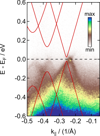
Figure S1: Experimental LEPD intensity map in comparison to simulation results for the LEPD signal for SnPc/SCG.

S. II Contribution of the Fermi-Dirac distribution to the temperature dependence of the LEPD intensity 

Figure S2 shows calculated Fermi-Dirac distribution functions $F(E)$ for $T=$300\text{\,}\mathrm{K}$$ and $T=$400\text{\,}\mathrm{K}$$, which corresponds to initial and final temperature of the static LEED and LEPD measurements on the temperature dependence of the diffraction intensities shown in Fig. 3(a). Both curves were convolved with a Gaussian to account for the energy resolution of $60\text{\,}\mathrm{m}\mathrm{e}\mathrm{V}$ of the experiment. The two dotted lines mark the energy interval used to evaluate the temperature dependence of the LEPD signal. The comparison of the integrals of the two Fermi-Dirac distribution functions in this energy interval shows that the heating of the electron gas can account for a maximum relative intensity change of the LEPD signal in the temperature range of $\approx$4.7\text{\,}\%$$. This value reduces to $\approx$4.6\text{\,}\%$$ if the density of state of graphite is taken into account Ooi et al. (2006). The value is significantly lower than the relative change in LEPD intensity of $\approx$ 40% observed in the experiment.

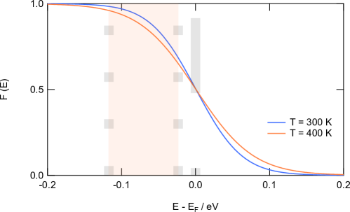
Figure S2: Calculated Fermi-Dirac distribution functions $F(E)$ to estimate its maximum contribution to the observed changes in the LEPD intensity as a function of temperature. To account for the finite energy resolution of the experiment, the distributions were convolved with a Gaussian with a FWHM of $60\text{\,}\mathrm{m}\mathrm{e}\mathrm{V}$.

S. III Calculation of the temperature increase of the SCG substrate due to absorption of the pump pulse 

The increase in temperature of the SCG substrate due to the pump pulse excitation and after complete thermalization of all electronic and lattice degrees of freedom has been calculated from the absorbed fluence by

$$\Delta T=\frac{0.06\cdot E_{\mathrm{pulse}}\cdot\cos(\Theta)}{V_{\mathrm{exc}}\cdot c_{\mathrm{graphite}}\cdot\rho_{\mathrm{graphite}}}\approx 16~{}\mathrm{K}$$ (1)

.

Here $E_{\mathrm{pulse}}=0.045~{}\upmu\mathrm{J}$ is the net energy deposited in the SCG substrate due to absorption calculated using the Fresnel equations. $\Theta=33^{\circ}$ is the incidence angle of the pump pulse, $c_{\mathrm{graphite}}=706~{}\mathrm{J~{}kg^{-1}K^{-1}}$ Picard et al. (2007) and $\rho_{\mathrm{graphite}}=2.1~{}\mathrm{g~{}cm^{-3}}$ are the specific heat and density of graphite, respectively. The factor 0.06 accounts for the probe pulse diameter ($d_{\mathrm{probe}}=50~{}\mathrm{\upmu m}$) being much smaller than the ($d_{\mathrm{pump}}=185~{}\mathrm{\upmu m}$), which guarantees that only the center of the excitation region is probed. The probed excitation volume $V_{\mathrm{exc}}=98~{}\mathrm{\upmu m^{3}}$ is given by the probe pulse diameter and the pump pulse penetration depth of $50~{}\mathrm{nm}$. The later value has been calculated from optical constants of graphite Djurišić and Li (1999).

S. IV Comparison of the ULEPD transients from $\pi$ and the $\pi^{*}$ band 

Figure S3 compares the ULEPD transients from the $\pi$ and the $\pi^{*}$ band on a semi-logarithmic scale, with the transient from the $\pi$ band inverted. In this representation of the data, it can be seen that for time delays between $1\text{\,}\mathrm{p}\mathrm{s}$ and $2\text{\,}\mathrm{p}\mathrm{s}$ the slopes of the two transients are virtually the same. We conclude that in this time window the the temporal evolution of both signals is governed by the same process, namely the decay of the hot carrier distribution. We used the integrated signals in this time interval to normalize the two transients in order to compensate for the differences in the matrix element for photoemission from the $\pi$ and the $\pi^{*}$ band Grüneis et al. (2008). By summing, we were able to separate quantitative information about the structural dynamics in the SnPc top layer from the carrier dynamics in the SCG substrate in a further step (see section S. V). Note that on longer time scales the $\pi$-band transient starts to deviate from the $\pi^{*}$-band transient as the structural dynamics in the adsorbate layer becomes more important.

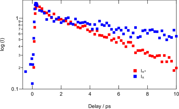
Figure S3: $\pi$ and the $\pi^{*}$ band transients in Fig. 2(d) of the main text in semi-logarithmic representation. The $\pi$-band transient was multiplied by a factor $(-1)$

S. V Summation of $\pi$-band and $\pi^{*}$-band transients 

The photoexcitation temporarily reduces the electron population in the $\pi$ band, so that the corresponding ULEPD signal intensity $I_{\pi}(\Delta t)$ contains information about the subsequent hole relaxation dynamics. Similarly, the ULEPD signal intensity $I_{\pi^{*}}(\Delta t)$ appears in the ULEPD data as soon as the $\pi^{*}$ band is occupied by photoexcitation. Due to charge conservation and neglecting differences in the photoemission matrix elements, $I_{\pi}(\Delta t)$ can be written as $I_{0\pi}-I_{\pi^{*}}(\Delta t)$, where $I_{0\pi}$ is the ULEPD signal from the $\pi$ band before photoexcitation. At the same time, both the transient ULEPD signals from the $\pi$ band and from the $\pi^{*}$ band are reduced by the (time-delay dependent) Debye-Waller factor DWF$(\Delta t)$ as soon as the SnPc layer is heated. The summation of the two signals, taking DWF$(\Delta t)$ into account, results in

$$[I_{0\pi}-I_{\pi^{*}}(\Delta t)]\cdot\text{DWF}(\Delta t)+I_{\pi^{*}}(\Delta t)\cdot\text{DWF}(\Delta t)=I_{0\pi}\cdot\text{DWF}(\Delta t)$$ (2)

so that a time-delay dependent signal remains that only governed by the DWF, i.e., the vibrational disorder in the adsorbate layer. To account for the differences in the photoemission matrix elements Grüneis et al. (2008); Stange et al. (2015), the transients were normalized before summation, as described in section S. IV.

S. VI Assignment of the temperature scale to the adsorbate transient in Fig. 3(b) 

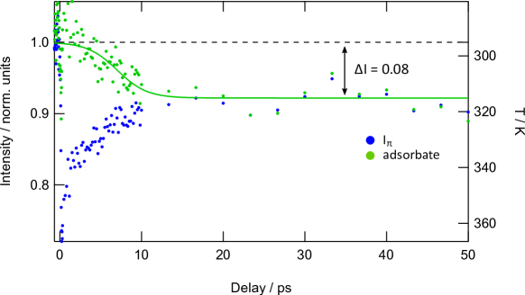
Figure S4: Total intensity changes in the ULEPD signal of the $\pi$ band overlaid with the ULEPD intensity changes associated with the excitation of the adsorbate layer (green line and data points). The intensity level before time zero was set to 1. For large time delays ($\Delta t>$20\text{\,}\mathrm{p}\mathrm{s}$$) the adsorbate layer transient was scaled to match the intensity level of the ULEPD signal of the $\pi$ band.

All data in Fig. 2(d) show difference intensities with respect to the ULEPD signal before excitation with the data being normalized to the average difference intensity in the time window between $1\text{\,}\mathrm{p}\mathrm{s}$ and $2\text{\,}\mathrm{p}\mathrm{s}$ (see section S.III). In order to relate the time-resolved data to the temperature scale derived from the analysis of the temperature dependent LEED and LEPD data in Fig. 3(a), we have to determine the relative intensity changes associated with the vibrational excitation of the adsorbate [green data points in Fig. 2(d)] with respect to the ULEPD signal from the $\pi$ band before excitation. The procedure is illustrates in Fig. S4. From the raw ULEPD data we extracted the total transient intensity change of the $\pi$ band signal and normalized this data set with respect to the intensity level before time zero (blue data points in Fig. S4). For large time delays, i.e., at time scales where the changes in the diffraction signal are given by the DWF, i.e., the vibrational excitation of the adsorbate layer, this data set yields a relative intensity change in the ULEPD signal of $\Delta I\approx$8\text{\,}\%$$. We then overlaid this data with the adsorbate lattice transient derived from the difference intensity data. Here the zero level of the data (which corresponds to the initial adsorbate state before excitation) is set to 1, the intensity level at large delays is re-scaled to match the intensity level of the raw data. The relative intensity changes can now be referred to the temperature dependent LEPD data in Fig. 3(a) yielding a scale for the time evolution of the temperature in the adsorbate layer.

References

- Erk et al. (2023) H. Erk, K. Opitz, P. Hein, S. Jauernik, and M. Bauer, J. Phys. Condens. Matter 35, 095501 (2023).
- Ooi et al. (2006) N. Ooi, A. Rairkar, and J. B. Adams, Carbon 44, 231 (2006).
- Picard et al. (2007) S. Picard, D. T. Burns, and P. Roger, Metrologia 44, 294 (2007).
- Djurišić and Li (1999) A. B. Djurišić and E. H. Li, Journal of Applied Physics 85, 7404 (1999).
- Grüneis et al. (2008) A. Grüneis, C. Attaccalite, A. Rubio, S. L. Molodtsov, D. V. Vyalikh, J. Fink, R. Follath, and T. Pichler, Phys. Status Solidi B Basic Res. 245, 2072 (2008).
- Stange et al. (2015) A. Stange, C. Sohrt, L. X. Yang, G. Rohde, K. Janssen, P. Hein, L.-P. Oloff, K. Hanff, K. Rossnagel, and M. Bauer, Phys. Rev. B 92, 184303 (2015).