$\Lambda$ polarization in very high energy heavy ion collisions as a probe of the Quark-Gluon Plasma formation and properties

Abstract

We have studied the spin polarization of $\Lambda$ hyperons in heavy ion collisions at center-of-mass energies $\sqrt{s_{\mathrm{NN}}}=200$ GeV and $\sqrt{s_{\mathrm{NN}}}=5.02$ TeV carried out at RHIC and LHC colliders. We have calculated the mean spin vector at local thermodynamic equilibrium, including all known first-order terms in the gradients of the thermo-hydrodynamic fields, assuming that the hadronization hypersurface has a uniform temperature. We have also included the feed-down contributions to the polarization of $\Lambda$ stemming from the decays of polarized $\Sigma^{*}$ and $\Sigma^{0}$ hyperons. The obtained results are in good agreement with the data. In general, the component of the spin vector along the global angular momentum, orthogonal to the reaction plane, shows strong sensitivity to the initial longitudinal flow velocity. Furthermore, the longitudinal component of the spin vector turns out to be very sensitive to the bulk viscosity of the plasma at the highest LHC energy. Therefore, the azimuthal dependence of spin polarization can effectively constrain the initial hydrodynamic conditions and the transport coefficients of the Quark Gluon Plasma.

I Introduction

After its measurement by STAR collaboration in 2017 Adamczyk et al. (2017), spin polarization has become an important probe in relativistic heavy ion collisions (for reviews, see Becattini and Lisa (2020); Becattini (2022); Becattini et al. (2024)). From a theoretical standpoint, the most successful approach is the hydrodynamic-statistical model where spin polarization is calculated at local thermodynamic equilibrium at hadronization when the Quark Gluon Plasma (QGP) gives rise to hadronic particles which rapidly decouple and freely stream to the detectors.

In the local equilibrium model, the sources of the spin polarization vector of fermions are the gradients of the hydro-thermodynamic fields, that is, temperature, velocity, and chemical potential. Even if, for some time, spin polarization was mostly connected to vorticity (more precisely, thermal vorticity Becattini et al. (2013); Fang et al. (2016); Florkowski et al. (2018); Weickgenannt et al. (2021)), it has become recently clear that also the symmetric gradient of the four-temperature (thermal shear tensor) and the gradient of the chemical potential Becattini et al. (2021a); Liu and Yin (2021); Yi et al. (2021) are responsible for a large contribution to local polarization, even though the global polarization is essentially determined by the thermal vorticity Alzhrani et al. (2022).

Particularly in very high energy collisions where the chemical potentials are negligible and the hadronization hypersurface $\Sigma$ can be approximated by an isothermal one, the mean spin polarization vector of Dirac fermions such as the $\Lambda$ hyperons with momentum $p$ is given by Becattini et al. (2021b) :

$$S^{\mu}(p)=-\epsilon^{\mu\rho\sigma\tau}p_{\tau}\frac{\int_{\Sigma}{\rm d}\Sigma\cdot p\;n_{F}(1-n_{F})\left[\omega_{\rho\sigma}+2\,\hat{t}_{\rho}\frac{p^{\lambda}}{\varepsilon}\Xi_{\lambda\sigma}\right]}{8mT_{H}\int_{\Sigma}{\rm d}\Sigma\cdot p\;n_{F}},$$ (1)

where $T_{H}$ is the hadronization temperature, $\hat{t}^{\mu}=\delta^{\mu}_{0}$ is the time unit vector in the QGP centre-of-mass frame, $\varepsilon=p\cdot\hat{t}$ and $n_{F}=[{\rm e}^{\beta\cdot p-\sum_{i}\mu_{i}/T}+1]^{-1}$ is the Fermi distribution (the chemical potentials can be taken as vanishing at the considered energies). The presence of a specific time vector is a manifestation of the dependence of the above formula on the specific hadronization hypersurface, which in turn is related to the non-conservation of the local equilibrium operator (see discussion in ref. Becattini et al. (2021a)). The tensors $\omega_{\mu\nu}$ and $\Xi_{\mu\nu}$ are the kinematic vorticity and shear, respectively:

$$\omega_{\mu\nu}=\frac{1}{2}\left(\partial_{\nu}u_{\mu}-\partial_{\mu}u_{\nu}\right),\qquad\Xi_{\mu\nu}=\frac{1}{2}\left(\partial_{\nu}u_{\mu}+\partial_{\mu}u_{\nu}\right).$$ (2)

The formulae (1) and (2) make it apparent that, unlike most other hadronic observables, spin polarization is sensitive to the flow velocity gradients at leading order. Therefore, polarization can be used as an important observable to constrain various medium parameters, as we will show in the present study.

Over the past few years, there have been several $\Lambda$ polarization numerical studies with the hydrodynamic model of the QGP based on thermal vorticity Wu et al. (2019); Florkowski et al. (2019); Huang et al. (2021); Lei et al. (2021); Serenone et al. (2021); Singh and Alam (2023) or including also the shear tensor contribution Becattini et al. (2021b); Fu et al. (2021); Florkowski et al. (2022); Alzhrani et al. (2022); Wu et al. (2022); Fu et al. (2022); Jiang et al. (2023a, b); Ribeiro et al. (2024); Yi et al. (2024). In this paper, we have carried out full numerical simulations of Au-Au at $\sqrt{s_{\mathrm{NN}}}=200$ GeV and Pb-Pb collisions at $\sqrt{s_{\mathrm{NN}}}=5020$ GeV and compared the obtained results to the available experimental data, employing up-to-date theoretical formulae for spin polarization. Furthermore, we have studied the sensitivity of spin polarization to the initial conditions and transport coefficients, specifically the shear and bulk viscosity. For the first time, we have included in a realistic hydrodynamic simulations the corrections due to the decay of polarized $\Sigma^{*}$ and $\Sigma^{0}$ (the so-called feed-down corrections) to the local polarization. Additionally, we have studied the impact of varying the initial longitudinal momentum flow in the initial state, showing that the local polarization along the total angular momentum is quite sensitive to it. It should be pointed out that such a dependence was studied in great detail in ref. Jiang et al. (2023b), for Au-Au collisions at $\sqrt{s_{\mathrm{NN}}}=27$ GeV. In order to avoid possible biases, we have employed two initial state models.

The paper is organized as follows. In section II we describe and validate the hydrodynamic simulation setup using two different initial state models. Section III is devoted to the study of feed-down corrections to the polarization vector, and in section IV, we calculate various polarization observables measured experimentally. Finally, we address the effect of the initial collective flow and viscosity on polarization in section V.

Notation

We adopt the natural units in this work, with $\hbar=c=K=1$. The Minkowskian metric tensor $g$ is ${\rm diag}(1,-1,-1,-1)$; for the Levi-Civita symbol we use the convention $\epsilon^{0123}=1$. We will use the relativistic notation with repeated indices assumed to be saturated.

II Numerical framework

The numerical setup used in this work builds upon the chain of codes vHLLE and SMASH Karpenko et al. (2014); Schäfer et al. (2022); Oliinychenko et al. (2023); Weil et al. (2016). Such a chain involves a pre-defined initial state, a 3+1D viscous hydrodynamic evolution of the produced dense medium, a fluid-to-particle transition (hadronization, or, more technically particlization), taking place at a surface of fixed energy density, followed by a Monte-Carlo hadronic sampling from the particlization hypersurface and a subsequent hadronic rescattering and resonance decays.

The hydrodynamic evolution is simulated with vHLLE code Karpenko et al. (2014), where the particlization hypersurface is reconstructed with Cornelius subroutine Huovinen and Petersen (2012). This hypersurface is used for the evaluation of $\Lambda$ polarization as well as for conventional Monte-Carlo sampling of hadrons using smash-hadron-sampler code sma (2023). Finally, SMASH Weil et al. (2016) handles rescatterings of the produced hadrons and decays of unstable resonances. We emphasize that spin degrees of freedom are not implemented in SMASH therefore, all the polarization results presented in this work (and so far in the literature) are solely based on formula (1) and the subsequent calculation of polarization transfer in the decay of resonances. The polarization calculations are performed using a dedicated code, hydro-foil, which is publicly available HYDROdynamic Freeze-Out IntegraLs . To conveniently handle all the chain stages, we have created a hybrid model based on the Python programming language and Snakemake Mölder et al. (2021); SMASH-vHLLE hybrid with Python .

Parameter	Description	@RHIC AuAu 200 GeV	@LHC PbPb 5020 GeV
$w[\text{fm}]$	Size of the initial hot spot	0.8	0.14
$\eta_{0}$	Size of the mid-rapidity plateau	2.2	2.7
$\sigma_{\eta}$	Space-time rapidity fall off width	0.9	1.2
$f$	Initial longitudinal flow fraction	0.15	0.15

Table 1: Values of the free parameters in the initialization of the hydrodynamic stage using superMC. For a detailed description of these initial condition parameters, see refs. Shen and Alzhrani (2020); Alzhrani et al. (2022).

Parameter	Description	@RHIC AuAu 200 GeV	@LHC PbPb 5020 GeV
$R[\text{fm}]$	Size of the initial hot spot	0.4	0.4
$\eta_{0}$	Size of the mid-rapidity plateau	1.5	2.4
$\sigma_{\eta}$	Space-time rapidity fall off width	1.4	1.4
$\eta_{M}$	Initial state tilt parameter	2.0	4.5

Table 2: Values of the free parameters in the initialization of hydrodynamic stage using 3D Glissando IS. For a detailed description of these initial condition parameters, see refs. Cimerman et al. (2021).

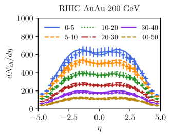
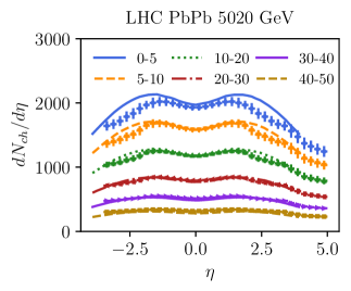
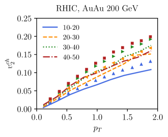
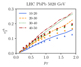
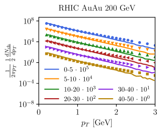
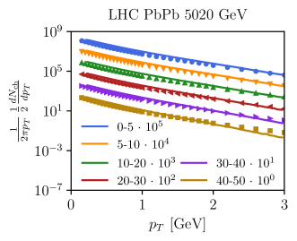
Figure 1: Comparison between model and data with superMC initial conditions. Left panels correspond to Au-Au collisions at $\sqrt{s_{\mathrm{NN}}}=200$ GeV at RHIC and the right ones to $\sqrt{s_{\mathrm{NN}}}=5020$ GeV Pb-Pb collisions at LHC. In the upper panels, we show the pseudo-rapidity distribution of charged hadrons, with data from Bearden et al. (2002) and Adam et al. (2017), the mid-panels show the elliptic flow of charged hadrons, data from refs. Adams et al. (2005) and Acharya et al. (2023), and the lower panels show the transverse momentum spectrum of charged hadrons, with data from refs. Adams et al. (2003) and Acharya et al. (2018).

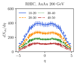
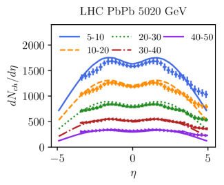
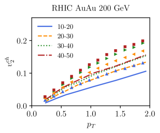
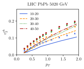
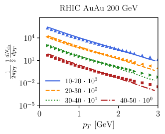
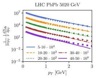
Figure 2: Comparison between model and experimental data with GLISSANDO initial conditions. Left panels correspond to Au-Au collisions at $\sqrt{s_{\mathrm{NN}}}=200$ GeV at RHIC and the right ones to $\sqrt{s_{\mathrm{NN}}}=5020$ GeV Pb-Pb collisions at LHC. In the upper panels, we show the pseudo-rapidity distribution of charged hadrons, the mid-panels show the elliptic flow of charged hadrons, and the lower panels show the transverse momentum spectrum of charged hadrons. The data are taken from the same references as in fig. 1.

As has been mentioned, we have used two Initial State (IS) models in this study. The first one is superMC, numerically implemented from scratch based on the formulae from Shen and Alzhrani (2020); Alzhrani et al. (2022). superMC is based on Glauber geometry with local energy and momentum conservation conditions and provides a $\sqrt{T_{A}T_{B}}$ scaling of the energy density similar to TrENTo Moreland et al. (2015) $p=0$ initial state. The second is a 3D extension of the initial state from Monte Carlo Glauber generator GLISSANDO Rybczynski et al. (2014). With either IS option, we have used the starting time of the fluid stage $\tau_{0}$ and shear viscosity to entropy density ratio $\eta/s$ values that are considered optimal to reproduce basic hadronic observables. In the case of superMC IS, the starting time of the fluid stage is $\tau_{0}=1$ fm/c and, unless otherwise stated, a fixed shear viscosity over entropy density ratio of $\eta/s=0.08$. In the case of 3D GLISSANDO IS, the initial time is $\tau_{0}=0.4$ fm/c, $\eta/s=0.08$ at RHIC energy and $\eta/s=0.1$ at LHC energy, which reflects a somewhat higher temperature range probed in heavy-ion collisions at the LHC. Instead, for the bulk viscosity over entropy density $\zeta/s$, we have used the temperature-dependent parametrization introduced in Schenke et al. (2020), referred to as parametrization III in section V (see eq. 12).

For $\sqrt{s_{\mathrm{NN}}}=200$ GeV energy, the values of the free parameters of the superMC IS model have been slightly modified with respect to those originally published in Shen and Alzhrani (2020); Alzhrani et al. (2022) to obtain an optimal description of the pseudo-rapidity distribution, elliptic flow of charged hadrons, and transverse momentum spectrum of identified hadrons. For $\sqrt{s_{\mathrm{NN}}}=5020$ GeV, a different optimal tuning has been found, with the values for both energies reported in Table 1. We have used an average initial state of 20k superMC events for the tuning. Figure 1 shows the results of our calculations compared to the experimental data. Baryon and electric charge currents do not play a significant role in collisions at the energies under consideration, so the free parameters associated with them, $\eta_{B0}$, $\sigma_{B\text{in}}$ and $\sigma_{B\text{out}}$, are the same as the ones reported in ref. Shen and Alzhrani (2020) for Au-Au collisions at $\sqrt{s_{\mathrm{NN}}}=200$ GeV.

The 3D extension of GLISSANDO initial state is taken from the study in ref.Cimerman et al. (2021), and it follows a parametrization previously reported in Bożek et al. (2015). Differently from ref. Cimerman et al. (2021), we have not computed the normalization of the initial state energy density by identifying the total energy of the fluid with the sum of energies of incoming participants. Instead, we have treated normalization as another free parameter and tuned it to fit charged hadron $dN/d\eta$ distribution. The resulting parameters are reported in Table 2, and figure 2 shows the results of our calculations. We generally have a very good agreement of transverse momentum spectra and pseudo-rapidity distributions of charged hadrons at various centralities but a less good agreement for their elliptic flow coefficient.

III Feed-down contribution to polarization

The hydrodynamic-statistical model predicts that all particles created by the particlization of the QGP are polarized. When unstable particles are produced in this stage, they transfer part of their polarization to their decay products. Therefore, secondary $\Lambda$s produced by decaying heavier particles or resonances are also polarized. The contribution to polarization owing to the secondary $\Lambda$s is called feed-down correction. As the experiments can subtract $\Lambda$s from long-lived weakly decaying hadrons, we only consider short-lived hadrons decaying through electromagnetic or strong interaction. Specifically we focus on $\Sigma^{*}\rightarrow\Lambda+\pi$ and $\Sigma^{0}\rightarrow\Lambda+\gamma$, which provide the predominant channels to secondary $\Lambda$ production.

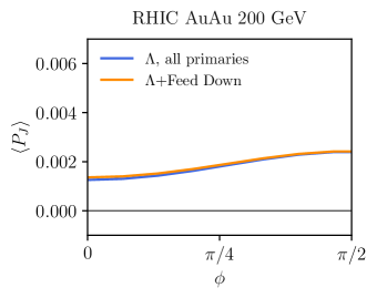
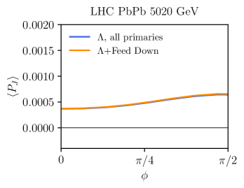
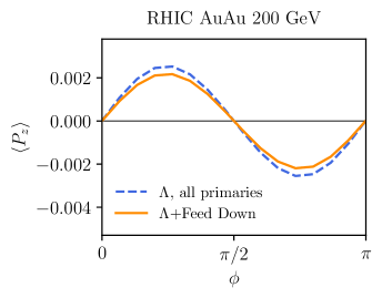
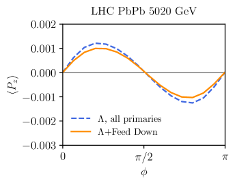
Figure 3: Feed-down corrections on the polarization along the angular momentum direction (upper panels) and along the beam line (lower panels). The solid line shows the polarization including the contribution of $\Sigma^{*}$ and $\Sigma^{0}$ while the dashed line the calculated polarization assuming that all $\Lambda$s are primaries. The simulations are in the centrality window 20-60% for RHIC and 30-50% for LHC.

The polarization transferred from a particle to its decay products in a two-body decay, has been extensively studied elsewhere Becattini et al. (2017); Xia et al. (2019); Becattini et al. (2019); herein, we briefly review it and describe the formulae used to compute it. Let us then consider the general decay $M\rightarrow\Lambda D$. The particle $M$ produced at hadronization is polarized, and, if it is a fermion, its mean spin vector can be obtained by simply rescaling the equation (1) Becattini et al. (2017); Xia et al. (2019); Becattini et al. (2019); Palermo and Becattini (2023):

$$S^{\mu}(p)=-\frac{S(S+1)}{3}\epsilon^{\mu\rho\sigma\tau}p_{\tau}\frac{\int_{\Sigma}{\rm d}\Sigma\cdot p\;n_{F}(1-n_{F})\left[\omega_{\rho\sigma}+2\,\hat{t}_{\rho}\frac{p^{\lambda}}{\varepsilon}\Xi_{\lambda\sigma}\right]}{2mT_{H}\int_{\Sigma}{\rm d}\Sigma\cdot p\;n_{F}},$$ (3)

where $S$ is the spin of the fermion. As it has been discussed, the produced $\Lambda$ is polarized. The spin vector ${\bf S}_{*}^{(M)}$ of the $\Lambda$ particle in its rest frame inherited from the mother particle is Becattini et al. (2019):

$${\bf S}_{*}^{(M)}({\bf p})=\frac{\int{\rm d}\Omega_{*}n({\bf P})F({\bf p},\Omega_{*}){\bf S}_{M\to\Lambda}({\bf P},{\bf p})}{\int{\rm d}\Omega_{*}n({\bf P})F({\bf p},\Omega_{*})}.$$ (4)

In the above formula, the solid angle $\Omega_{*}$ is in the rest frame of the mother particle, ${\bf p}$ and ${\bf P}$ are the momenta of $\Lambda$ and $M$ respectively in the QGP frame and ${\bf S}_{M\to\Lambda}$ is a “spin-transfer” vector function depending on the decay. For the aforementioned decays, they read:

$${\bf S}_{\Sigma^{*}\to\Lambda}({\bf P},{\bf p}) =\frac{2}{5}\left({\bf S}_{*\Sigma^{*}}({\bf P})-\frac{1}{2}\hat{{\bf p}}\cdot{\bf S}_{*\Sigma^{*}}({\bf P})\;\hat{{\bf p}}\right)$$ (5a)

$${\bf S}_{\Sigma^{0}\to\Lambda}({\bf P},{\bf p}) =-\hat{{\bf p}}\cdot{\bf S}_{*\Sigma^{0}}({\bf P})\;\hat{{\bf p}}$$ (5b)

where ${\bf S}_{*\Sigma^{*}}$ and ${\bf S}_{*\Sigma^{0}}$ are the spin vectors of the mother particles in the mother’s rest frame, which can be computed with eq. (3). The function $F({\bf p},\Omega_{*})$ is given by:

$$F({\bf p},\Omega_{*})=\frac{m_{\Lambda}^{3}(\varepsilon_{*\Lambda}+\varepsilon_{\Lambda})\left[(\varepsilon_{*\Lambda}+\varepsilon_{\Lambda})^{2}-(\varepsilon_{\Lambda}\varepsilon_{*\Lambda}+{\bf p}\cdot{\bf p}_{*}+m_{\Lambda}^{2})\right]}{\varepsilon_{*\Lambda}(\varepsilon_{\Lambda}\varepsilon_{*\Lambda}+{\bf p}\cdot{\bf p}_{*}+m_{\Lambda}^{2})^{3}},$$ (6)

where $\varepsilon_{*\Lambda}$ and ${\bf p}_{*}$ are the energy and the momentum of the $\Lambda$ particle in the mother’s rest frame. Finally, the function $n({\bf P})$ is the momentum spectrum of $M$ in the QGP frame obtained from the Cooper-Frye prescription:

$$n({\bf P})=\frac{{\rm d}N}{{\rm d}^{3}{\rm P}}=\frac{1}{\varepsilon_{P}}\int{\rm d}\Sigma\cdot P\;\frac{1}{{\rm e}^{\beta\cdot P-\mu/T}+1}.$$ (7)

All the integrals in equation (4) are evaluated in the hydro-foil code.

To determine the overall $\Lambda$’s polarization, one should know the fraction of primary $\Lambda$s and those from the considered decays. Although such fractions are, in principle, momentum dependent, here, for simplicity, we assume that they are constant and use the numbers quoted in ref. Becattini et al. (2019) estimated by using the statistical hadronization model: the fraction of primary $\Lambda$, at very high energy, is $f_{P}=0.243$ whereas for the secondary $\Lambda$ one has respectively $f_{\Sigma^{*}}=0.359$ and $f_{\Sigma^{0}}=0.275\times 0.6=0.165$, where the $0.6$ takes into account that only $\approx 60\%$ of the $\Sigma_{0}$ are primary; other sources are neglected. Finally, the total $\Lambda$’s spin vector in its rest frame is calculated by normalizing it accordingly:

$${\bf S}_{*}^{\text{tot}}(p)=\frac{f_{P}{\bf S}_{*}^{\text{P}}({\bf p})+f_{\Sigma^{*}}{\bf S}_{*}^{(\Sigma^{*})}({\bf p})+f_{\Sigma^{0}}{\bf S}_{*}^{(\Sigma^{0})}({\bf p})}{f_{P}+f_{\Sigma^{*}}+f_{\Sigma^{0}}},$$ (8)

where ${\bf S}_{*}^{\text{P}}({\bf p})$ is the spin polarization vector of primary $\Lambda$s, determined by boosting the spin vector in the eq. (1) back to the $\Lambda$ rest frame and ${\bf S}_{*}^{(\Sigma^{*})}({\bf p})$, ${\bf S}_{*}^{(\Sigma_{0})}({\bf p})$ are calculated by means of the eq. (4).

Figure 3 shows the effect of the feed-down contribution to the component of the polarization vector along the angular momentum (henceforth referred to as transverse) and along the beamline (henceforth referred to as longitudinal) $\langle P_{J,z}\rangle=2\langle S_{J,z}\rangle$ by comparing it to a calculation where all $\Lambda$ are assumed to be primary. The simulations are performed with the superMC initial conditions. As already remarked in Xia et al. (2019); Becattini et al. (2019) the combination in (8) results in an accidental approximate cancellation so that the total polarization is almost the same as though the $\Lambda$s were only primary. More precisely, the feed-down correction implies a $\approx 10\%$ reduction to the full primary case for the longitudinal component and $\approx 3\%$ for the transverse component. So, even with the contribution from the thermal shear tensor included, which was not the case in refs. Xia et al. (2019); Becattini et al. (2019), we confirm the previous conclusion that adding feed-down corrections does not significantly change the polarization with respect to the simple assumption of an entirely primary production.

IV Polarization at very high energy: results

We will now present the results of our calculation and their comparison with the data. In our calculations, feed-down corrections are always included; even though they are small corrections to the assumption of pure primary production, they certainly improve the accuracy of theoretical predictions. In the plots, we show the proper polarization vector $P^{\mu}(p)=S_{*}^{\mu}(p)/S$ where $S$ is the spin of the particles and $S_{*}^{\mu}(p)$ is the mean spin vector in the $\Lambda$’s rest frame (hence, for $\Lambda$ hyperon $P^{\mu}=2S_{*}^{\mu}$). The value of the $\Lambda$ decay constant has been set to $\alpha_{\Lambda}=0.732$ to compare with experiments Zyla et al. (2020).

Simulations have been carried out using averaged initial states, which, as has been discussed in section II, were defined by the models superMC and GLISSANDO. For the superMC IS, the initial state was generated by averaging 20k samples. For GLISSANDO IS, 1k and 3k samples were used. In all cases, we compute polarization of $\Lambda$s in the rapidity window $\eta\in[-1,1]$ to match experimental measurements. Polarization as a function of the azimuthal angle $\langle P_{z}(\phi)\rangle$ and $\langle P_{J}(\phi)\rangle$ are integrated over the $p_{T}$ range $(0,6)$ GeV weighted by the $\Lambda$ spectrum, whereas $\langle P_{z}\sin 2\phi\rangle$ is the mean over the azimuthal angle $\phi$.

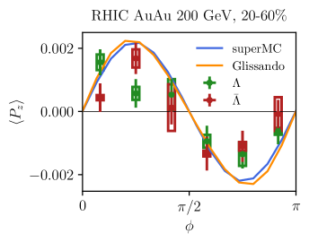
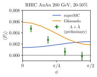
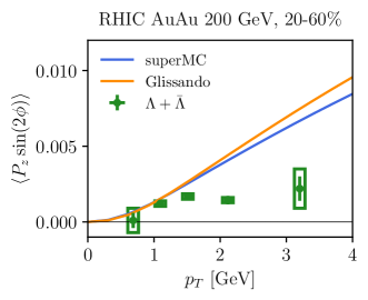
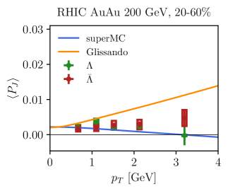
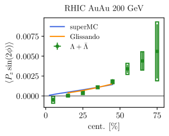
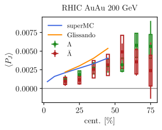
Figure 4: Comparison between theoretical calculations and experimental data for Au-Au collisions at 200 GeV. Top panels: azimuthal angle dependence of longitudinal and transverse polarization. The middle panels show the transverse momentum dependence of $\langle P_{z}\sin(2\phi)\rangle$ and $\langle P_{J}\rangle$, and the bottom panels show their dependence on centrality. For the top and middle panels, the simulations are carried in the centrality 20-60%. The data are taken from refs. Niida (2019); Adam et al. (2018, 2019).

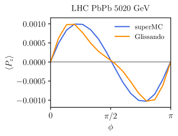
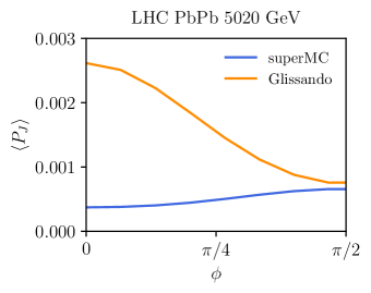
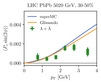
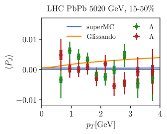
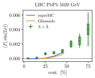
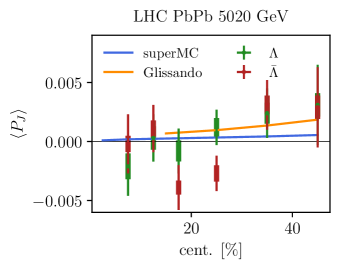
Figure 5: Comparison between theoretical calculations and experimental data for Pb-Pb collisions at 5020 GeV. Top panels: azimuthal angle dependence of transverse and longitudinal polarization. The middle panels show the transverse momentum dependence of $\langle P_{z}\sin(2\phi)\rangle$ and $\langle P_{J}\rangle$, and the bottom panels show their dependence on centrality. For the top and middle panels, the simulations are carried in the centrality 30-50%. The data are taken from refs. Acharya et al. (2020, 2022) .

For $\sqrt{s_{\mathrm{NN}}}=200$ Gev Au-Au collisions, the results are shown in figure 4 where the data points have been taken from refs. Niida (2019); Adam et al. (2018, 2019). The centrality reported in the titles in the top and middle panels refers to the data, whereas simulations have always been carried out at 20-60%. Our model describes well the longitudinal component of polarization $P_{z}$, as can be seen in the figures, although we overshoot the data in the high $p_{T}$ region. This result confirms the previous finding Becattini et al. (2021b) that the formula (1) reproduces the data, essentially solving the so-called polarization sign puzzle. The difference between our calculations and those in ref. Alzhrani et al. (2022) using the same initial conditions superMC is owing to the use of the isothermal hadronization assumption as well as a difference in the expression of energy $\varepsilon$ in (1), which is $p\cdot\hat{t}$ in our case and $p\cdot u$ in ref. Alzhrani et al. (2022).

While GLISSANDO and superMC provide similar predictions for the longitudinal polarization, they differ for the transverse component and especially for its azimuthal angle dependence. GLISSANDO IS predicts the correct dependence of $\langle P_{J}\rangle$ on the azimuthal angle, although with an overestimated polarization. Instead, superMC does not get the slope right, although the global polarization (middle-right panel) is well reproduced; similar observations were reported in Alzhrani et al. (2022) which, as has been mentioned, used the same IS model. In general, as it can be seen in the other plots in figure 4 GLISSANDO predicts a larger $P_{J}$ than superMC as a function of $p_{T}$ and centrality.

A substantial difference in the implementation of longitudinal hydrodynamic initial conditions causes the discrepancy between GLISSANDO and superMC in the transverse component $P_{J}$. Indeed, it should be stressed that the transverse component of the polarization is sensitive to the longitudinal velocity (see the equation (1)) whereas the longitudinal component of the polarization is sensitive to the transverse velocity Becattini and Karpenko (2018); Voloshin (2018); Jiang et al. (2023b). While the hydrodynamic initial conditions in the transverse plane are strongly constrained by the observed transverse momentum spectra and their azimuthal anisotropies, initial longitudinal flow conditions are not accurately known. Indeed, superMC IS parametrization entails a non-vanishing $\tau$-$\eta$ component of the energy-momentum tensor, hence a non-vanishing initial longitudinal velocity, $u^{\eta}\neq 0$, whereas GLISSANDO IS initializes $u^{\eta}=0$. This difference will be addressed in more detail in the next section.

The results of our calculations for Pb-Pb collisions at $\sqrt{s_{\mathrm{NN}}}=5020$ GeV are shown in figure 5 along with the ALICE data Acharya et al. (2020, 2022). The top panels show the theoretical predictions of longitudinal and transverse polarization as a function of the azimuthal angle: no data is available for these observables yet. In the middle panels, once again, the centrality reported in the title refers to the data, whereas simulations have been carried out at 30-50%. The predicted longitudinal polarization is smaller than at RHIC energy by a factor of $\approx 2$ with both IS conditions. It can be seen that our calculations for the longitudinal polarization with both IS models agree with each other, as well as with the data (when available). On the other hand, like at RHIC energy, the predictions of the two IS models used are very different for the transverse polarization. The measurement of $P_{J}$ at this energy has significantly larger error bars than RHIC energy, so no definite conclusion can be drawn from comparing the predictions with the data.

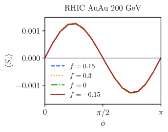
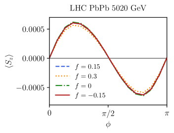
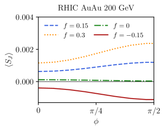
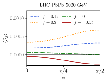
Figure 6: Azimuthal angle dependence of $S_{z}$ (upper panels) and $S_{J}$ (lower panels) for different values of the parameter $f$ in the superMC initial state model. RHIC simulations are made in 20-60% centrality, whereas LHC at 30-50%.

V Sensitivity to initial conditions and transport coefficients

In this section, we delve into the capability of spin polarization as a probe of the hydrodynamic initial conditions and the transport coefficients of the QGP. We already mentioned that the two IS used differ in the predictions of the transverse polarization $P_{J}$, which reflects different initial conditions for the longitudinal momentum density. To make this apparent, we have studied the sensitivity of $P_{z}(\phi)$ and $P_{J}(\phi)$ to the parameter $f$ in the superMC IS model. This parameter determines the initial values of the components of the energy-momentum tensor in the Milne coordinates as follows:

$$T^{\tau\tau} =\rho\cosh(f\,y_{CM})$$ (9a)

$$T^{\tau\eta} =\frac{\rho}{\tau}\sinh(f\,y_{CM})$$ (9b)

where $\rho$ is the local energy density distribution and $y_{CM}$ is the center of mass rapidity (for a full description of these quantities, see ref. Alzhrani et al. (2022)). Therefore, the value of $f$ characterizes the initial longitudinal momentum density $T^{\tau\eta}$, thus driving the initial longitudinal flow and the fireball’s total angular momentum. The latter affects the transverse component of the polarization $P_{J}$ as already discussed. We note that the equations (9) have been considered also in ref. Jiang et al. (2023b), where the dependence on $f$ of the $\Lambda$ polarization has been studied at $\sqrt{s_{\mathrm{NN}}}=27$ GeV. Figure 6 shows both transverse and longitudinal polarization from hydrodynamic simulations of Au-Au and Pb-Pb collisions initialized with different values of $f$. As expected, while the longitudinal component is almost insensitive to $f$, the transverse component changes significantly in magnitude, slope, and even sign. This sensitivity makes it possible to use local transverse polarization to discriminate between different models of initial longitudinal conditions and to pin down the amount of initial longitudinal momentum density. For the case at hand, the curves are shown in figure 6, and the results from GLISSANDO IS presented in the section IV seem to favor the option $u^{\eta}=0$, implemented by $f=0$, which is the only one yielding at least the correct sign of the slope of the function $P_{J}(\phi)$ at RHIC.

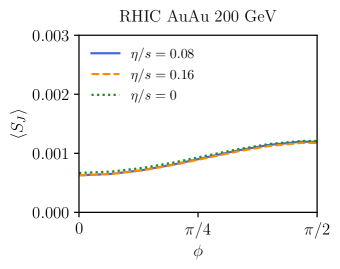
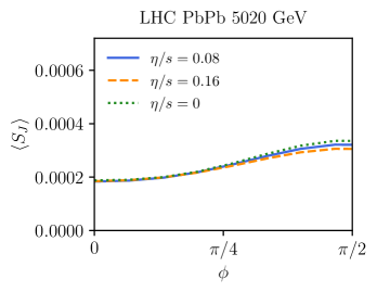
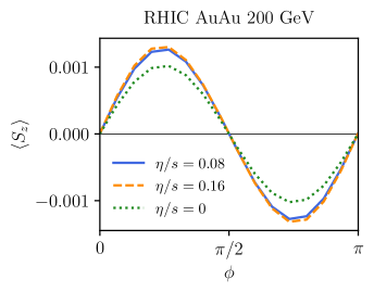
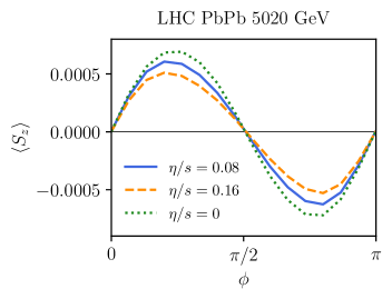
Figure 7: Transverse and longitudinal components of the spin vector as a function of the azimuthal angle $\phi$ for various values of the shear viscosity over entropy density. The centrality window is 20-60% for RHIC and 30-50% for LHC.

We have also studied the dependence of the polarization on the shear viscosity and the bulk viscosity. In figure 7, the transverse and longitudinal components of the spin vector of primary $\Lambda$s with the superMC IS, averaged over the same kinematic intervals as in section II, are shown at RHIC and LHC energies for different constant ratios of $\eta/s$. The transverse component is almost insensitive to the shear viscosity, while the longitudinal component has a limited sensitivity. Interestingly, we notice that while at RHIC energies, a larger viscosity enhances the signal, at LHC, it slightly reduces it.

Conversely, bulk viscosity has a sizeable effect on polarization, especially at high energy, in agreement with previous observations Palermo et al. (2023). We have used three different parametrizations of bulk viscosity as a function of temperature Bobek and Karpenko (2022). The first one, dubbed as “Parametrization I” was introduced in ref. Ryu et al. (2018):

$$\zeta/s=\begin{cases}c_{1}+0.08\exp\left[\frac{T/T_{p}-1}{0.0025}\right]+0.22\exp\left[\frac{T/T_{p}-1}{0.0022}\right]&\quad T<T_{p}\\ c_{2}+27.55\left(T/T_{p}\right)-13.77\left(T/T_{p}\right)^{2}&\quad T_{p}<T<T_{P}\\ c_{3}+0.9\exp\left[\frac{-\left(T/T_{p}-1\right)}{0.0025}\right]+0.25\exp\left[\frac{-\left(T/T_{p}-1\right)}{0.13}\right]&\quad T>T_{P},\end{cases}$$ (10)

where $T_{p}=180$ MeV, $T_{P}=200$ MeV, $c_{1}=0.03$, $c_{2}=-13.45$ and $c_{3}=0.001$. The second parametrization was introduced in ref. Schenke et al. (2019):

$$\zeta/s=\begin{cases}B_{\mathrm{norm}}\exp\left[-\left(\frac{T-T_{\mathrm{peak}}}{T_{\mathrm{width}}}\right)^{2}\right]&T<T_{\mathrm{peak}}\\ B_{\mathrm{norm}}\frac{B_{\mathrm{width}}^{2}}{(T/T_{\mathrm{peak}}-1)^{2}+B_{\mathrm{width}}^{2}}&T>T_{\mathrm{peak}},\end{cases}$$ (11)

where $T_{\mathrm{peak}}=165$ MeV, $B_{\mathrm{norm}}=0.24$, $B_{\mathrm{width}}=1.5$ and $T_{\mathrm{width}}=50$ MeV. The last parametrization, dubbed as “Parametrization III”, was introduced in ref. Schenke et al. (2020) and it reads:

$$\zeta/s=\begin{cases}B_{\rm n}\exp\left[-\left(\frac{T-T_{\mu}}{B_{1}}\right)^{2}\right]&T<T_{\mu}\\ B_{\rm n}\exp\left[-\left(\frac{T-T_{\mu}}{B_{2}}\right)^{2}\right]&T>T_{\mu},\end{cases}$$ (12)

where $B_{\rm n}=0.13$, $B_{1}=10$ MeV, $B_{2}=120$ MeV and $T_{\mu}=160$ MeV. These parametrizations are shown in figure 8, where it can be seen that parametrization I has the sharpest peak around the transition temperature, the other two featuring a broader peak. In parametrization II, $\zeta/s$ is always larger than parametrization III.

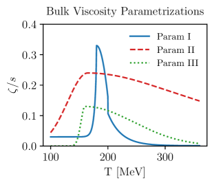
Figure 8: The temperature dependence of the bulk viscosity over entropy density ratio is used in this work.

The components of the mean spin vector - of primary particles only - along the angular momentum direction and the beam axis are shown in figure 9 in Au-Au collisions at $\sqrt{s_{\mathrm{NN}}}=200$ GeV and Pb-Pb collisions at $\sqrt{s_{\mathrm{NN}}}=5020$ GeV for all the different parametrizations and using the superMC IS (with $f=0.15$ as in the initial tuning). Bulk viscosity’s effect on polarization is mild at $\sqrt{s_{\mathrm{NN}}}=200$ GeV: different parametrizations slightly change the magnitude of the polarization signal compared to the case of $\zeta=0$, but their difference is well within the experimental errors. Instead, surprisingly, at $\sqrt{s_{\mathrm{NN}}}=5020$ GeV the effect of bulk viscosity is dramatic: the longitudinal polarization flips/changes sign when bulk viscosity is introduced, and the difference between the three parametrizations is large. Identifying a single effect responsible for such different behavior at RHIC and LHC energies is hard. A possible explanation could be that the higher average temperature and the longer lifetime of the QGP at the LHC energy make the role of bulk viscosity more important.

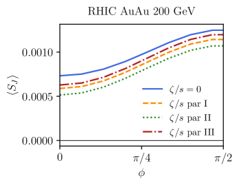
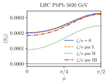
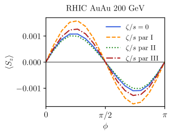
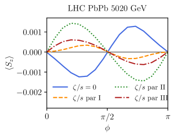
Figure 9: Transverse and longitudinal components of the spin vector as a function of the azimuthal angle $\phi$ for various bulk viscosity parametrization at $\sqrt{s_{\mathrm{NN}}}=200$ GeV (20-60% centrality) and $\sqrt{s_{\mathrm{NN}}}=5020$ GeV (30-50% centrality).

To investigate this phenomenon in more detail, we have computed the contribution of different hydrodynamic gradients to the spin vector for primary $\Lambda$s. Referring to eq. (1), the kinematic vorticity and shear can be decomposed in terms of acceleration $A^{\mu}=u\cdot\partial u^{\mu}$, angular velocity $\omega^{\mu}=-1/2\,\epsilon^{\mu\nu\rho\sigma}\partial_{\rho}u_{\nu}u_{\sigma}$, shear stress tensor $\sigma^{\mu\nu}$ and expansion scalar $\theta$ so that:

$$\omega_{\mu\nu} =\epsilon_{\mu\nu\rho\sigma}\omega^{\rho}u^{\sigma}+\frac{1}{2}\left(A_{\mu}u_{\nu}-A_{\nu}u_{\mu}\right),$$ (13)

$$\Xi_{\mu\nu} =\frac{1}{2}\left(A_{\mu}u_{\nu}+A_{\nu}u_{\mu}\right)+\sigma_{\mu\nu}+\frac{1}{3}\theta\Delta_{\mu\nu},$$ (14)

where $\Delta^{\mu\nu}=g^{\mu\nu}-u^{\mu}u^{\nu}$. Defining $\nabla_{\mu}=\Delta_{\mu\nu}\partial^{\nu}$, one has:

$$\theta =\nabla\cdot u=\partial\cdot u,$$

$$\sigma_{\mu\nu} =\frac{1}{2}\left(\nabla_{\mu}u_{\nu}+\nabla_{\nu}u_{\mu}\right)-\frac{1}{3}\theta\Delta_{\mu\nu}.$$

By decomposing the tensors $\omega_{\mu\nu}$ and $\Xi_{\mu\nu}$ in the formula (1) according to the above equations it is possible to identify different contributions to the spin polarization vector:

$$S^{\mu}_{A_{\omega}}=-\epsilon^{\mu\nu\rho\sigma}p_{\sigma}\frac{\int_{\Sigma}{\rm d}\Sigma\cdot p\,n_{F}(1-n_{F})\;A_{\nu}u_{\rho}}{8mT_{H}\int_{\Sigma}{\rm d}\Sigma\cdot p\,n_{F}},$$ (15a)

$$S^{\mu}_{\omega}=\frac{\int_{\Sigma}{\rm d}\Sigma\cdot p\,n_{F}(1-n_{F})\;\left[\omega^{\mu}u\cdot p-u^{\nu}\omega\cdot p\right]}{4mT_{H}\int_{\Sigma}{\rm d}\Sigma\cdot p\,n_{F}},$$ (15b)

$$S^{\mu}_{A_{\Xi}}=-\epsilon^{\mu\rho\sigma\tau}\hat{t}_{\rho}\frac{p_{\tau}}{\varepsilon}\frac{\int_{\Sigma}{\rm d}\Sigma\cdot p\;n_{F}(1-n_{F})\left[u_{\sigma}A\cdot p+A_{\sigma}u\cdot p\right]}{8mT_{H}\int_{\Sigma}{\rm d}\Sigma\cdot p\;n_{F}},$$ (15c)

$$S^{\mu}_{\sigma}=-\epsilon^{\mu\rho\sigma\tau}\hat{t}_{\rho}p_{\tau}\frac{p^{\lambda}}{\varepsilon}\frac{\int_{\Sigma}{\rm d}\Sigma\cdot p\;n_{F}(1-n_{F})\sigma_{\lambda\sigma}}{4mT_{H}\int_{\Sigma}{\rm d}\Sigma\cdot p\;n_{F}},$$ (15d)

$$S^{\mu}_{\theta}=-\epsilon^{\mu\rho\sigma\tau}\hat{t}_{\rho}p_{\tau}\frac{p^{\lambda}}{\varepsilon}\frac{\int_{\Sigma}{\rm d}\Sigma\cdot p\;n_{F}(1-n_{F})\theta\Delta_{\lambda\sigma}}{12mT_{H}\int_{\Sigma}{\rm d}\Sigma\cdot p\;n_{F}}.$$ (15e)

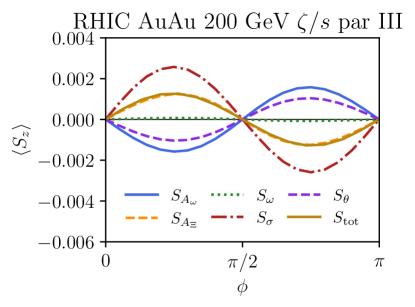
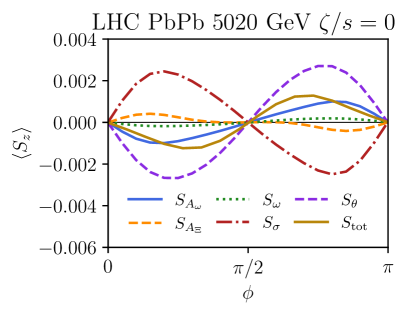
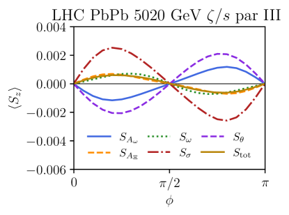
Figure 10: Contributions to the spin polarization vector (see eq. 15), for primary $\Lambda$’s at RHIC (centrality window 20-60%), and LHC energy (centrality window 30-50%).

We have computed the above components for two bulk viscosities: parametrization III of $\zeta/s$ in equation (12) and for vanishing $\zeta/s=0$, see figure 10. In Au-Au collisions at RHIC energy, the contribution from angular velocity is almost vanishing, according to previous findings Karpenko and Becattini (2019) and contrary to the naive lore, which identifies rotation as the main source of polarization. Overall, for parametrization III, the amplitude of both $S_{\sigma}$ and $S_{\theta}$ is smaller than for $\zeta=0$ case, but their sum is approximately zero and the total polarization is almost unaffected. On the other hand, in Pb-Pb collisions at LHC energy, the situation is more complicated. Without bulk viscosity, $S_{\theta}$ seemingly cancels $S_{\sigma}$, and $S_{A_{\omega}}$ dictates the (negative) sign of the polarization harmonic. Turning on the bulk viscosity, not only do $S_{\theta}$ and $S_{\sigma}$ get smaller in magnitude, but also $S_{\omega}$ and $S_{A_{\Xi}}$ significantly change, resulting in the change of sign of the oscillation pattern.

VI Conclusions

In summary, we have presented an analysis of spin polarization of $\Lambda$ produced in Au-Au collisions at $\sqrt{s_{\mathrm{NN}}}=200$ GeV and in Pb-Pb collisions at $\sqrt{s_{\mathrm{NN}}}=5020$ GeV, using two different initial state models. By assuming that the particlization hypersurface is isothermal and including the feed-down corrections, we have found a good agreement between the data and the predictions of the hydrodynamic-statistical model, thus confirming the previous finding Becattini et al. (2021b) that isothermal assumption is an important point to reproduce the data. Calculations with GLISSANDO initial state model are in good agreement with the data while superMC initial state model reproduces the longitudinal component and the global transverse polarization but fails to reproduce the transverse polarization as a function of the azimuthal angle. Transverse polarization is very sensitive to the initial longitudinal flow, and our results seem to favor a scenario with initial boost-invariant flow velocity.

We have shown that the longitudinal polarization is very sensitive to bulk viscosity at the highest collision energy and almost insensitive to the shear viscosity. At the LHC energy, the presence of bulk viscosity flips the sign of the polarization along the beam direction compared to a scenario with ideal fluid evolution.

Altogether, these results demonstrate that spin polarization, and in particular its azimuthal angle dependence, can be used as a very effective probe of initial conditions and transport coefficients of the Quark-Gluon plasma.

References

- Adamczyk et al. (2017) L. Adamczyk et al. (STAR), Nature 548, 62 (2017), arXiv:1701.06657 [nucl-ex] .
- Becattini and Lisa (2020) F. Becattini and M. A. Lisa, Ann. Rev. Nucl. Part. Sci. 70, 395 (2020), arXiv:2003.03640 [nucl-ex] .
- Becattini (2022) F. Becattini, Rept. Prog. Phys. 85, 122301 (2022), arXiv:2204.01144 [nucl-th] .
- Becattini et al. (2024) F. Becattini, M. Buzzegoli, T. Niida, S. Pu, A.-H. Tang, and Q. Wang, (2024), arXiv:2402.04540 [nucl-th] .
- Becattini et al. (2013) F. Becattini, V. Chandra, L. Del Zanna, and E. Grossi, Annals Phys. 338, 32 (2013), arXiv:1303.3431 [nucl-th] .
- Fang et al. (2016) R.-h. Fang, L.-g. Pang, Q. Wang, and X.-n. Wang, Phys. Rev. C 94, 024904 (2016), arXiv:1604.04036 [nucl-th] .
- Florkowski et al. (2018) W. Florkowski, A. Kumar, and R. Ryblewski, Phys. Rev. C 98, 044906 (2018), arXiv:1806.02616 [hep-ph] .
- Weickgenannt et al. (2021) N. Weickgenannt, E. Speranza, X.-l. Sheng, Q. Wang, and D. H. Rischke, Phys. Rev. Lett. 127, 052301 (2021), arXiv:2005.01506 [hep-ph] .
- Becattini et al. (2021a) F. Becattini, M. Buzzegoli, and A. Palermo, Phys. Lett. B 820, 136519 (2021a), arXiv:2103.10917 [nucl-th] .
- Liu and Yin (2021) S. Y. F. Liu and Y. Yin, JHEP 07, 188 (2021), arXiv:2103.09200 [hep-ph] .
- Yi et al. (2021) C. Yi, S. Pu, and D.-L. Yang, Phys. Rev. C 104, 064901 (2021), arXiv:2106.00238 [hep-ph] .
- Alzhrani et al. (2022) S. Alzhrani, S. Ryu, and C. Shen, Phys. Rev. C 106, 014905 (2022), arXiv:2203.15718 [nucl-th] .
- Becattini et al. (2021b) F. Becattini, M. Buzzegoli, G. Inghirami, I. Karpenko, and A. Palermo, Phys. Rev. Lett. 127, 272302 (2021b), arXiv:2103.14621 [nucl-th] .
- Fu et al. (2021) B. Fu, S. Y. F. Liu, L. Pang, H. Song, and Y. Yin, Phys. Rev. Lett. 127, 142301 (2021), arXiv:2103.10403 [hep-ph] .
- Wu et al. (2022) X.-Y. Wu, C. Yi, G.-Y. Qin, and S. Pu, Phys. Rev. C 105, 064909 (2022), arXiv:2204.02218 [hep-ph] .
- Jiang et al. (2023a) Z.-F. Jiang, X.-Y. Wu, H.-Q. Yu, S.-S. Cao, and B.-W. Zhang, Acta Phys. Sin. 72, 072504 (2023a).
- Jiang et al. (2023b) Z.-F. Jiang, X.-Y. Wu, S. Cao, and B.-W. Zhang, Phys. Rev. C 108, 064904 (2023b), arXiv:2307.04257 [nucl-th] .
- Ribeiro et al. (2024) V. H. Ribeiro, D. Dobrigkeit Chinellato, M. A. Lisa, W. Matioli Serenone, C. Shen, J. Takahashi, and G. Torrieri, Phys. Rev. C 109, 014905 (2024), arXiv:2305.02428 [hep-ph] .
- (19) Chun Shen, private communication.
- Wu et al. (2019) H.-Z. Wu, L.-G. Pang, X.-G. Huang, and Q. Wang, Phys. Rev. Research. 1, 033058 (2019), arXiv:1906.09385 [nucl-th] .
- Florkowski et al. (2019) W. Florkowski, A. Kumar, R. Ryblewski, and A. Mazeliauskas, Phys. Rev. C 100, 054907 (2019), arXiv:1904.00002 [nucl-th] .
- Huang et al. (2021) X.-G. Huang, J. Liao, Q. Wang, and X.-L. Xia, Lect. Notes Phys. 987, 281 (2021), arXiv:2010.08937 [nucl-th] .
- Lei et al. (2021) A. Lei, D. Wang, D.-M. Zhou, B.-H. Sa, and L. P. Csernai, Phys. Rev. C 104, 054903 (2021), arXiv:2110.13485 [nucl-th] .
- Serenone et al. (2021) W. M. Serenone, J. a. G. P. Barbon, D. D. Chinellato, M. A. Lisa, C. Shen, J. Takahashi, and G. Torrieri, Phys. Lett. B 820, 136500 (2021), arXiv:2102.11919 [hep-ph] .
- Singh and Alam (2023) S. K. Singh and J.-e. Alam, Eur. Phys. J. C 83, 585 (2023), arXiv:2110.15604 [hep-ph] .
- Florkowski et al. (2022) W. Florkowski, A. Kumar, A. Mazeliauskas, and R. Ryblewski, Phys. Rev. C 105, 064901 (2022), arXiv:2112.02799 [hep-ph] .
- Fu et al. (2022) B. Fu, L. Pang, H. Song, and Y. Yin, (2022), arXiv:2201.12970 [hep-ph] .
- Yi et al. (2024) C. Yi, X.-Y. Wu, D.-L. Yang, J.-H. Gao, S. Pu, and G.-Y. Qin, Phys. Rev. C 109, L011901 (2024), arXiv:2304.08777 [hep-ph] .
- Karpenko et al. (2014) I. Karpenko, P. Huovinen, and M. Bleicher, Comput. Phys. Commun. 185, 3016 (2014), arXiv:1312.4160 [nucl-th] .
- Schäfer et al. (2022) A. Schäfer, I. Karpenko, X.-Y. Wu, J. Hammelmann, and H. Elfner (SMASH), Eur. Phys. J. A 58, 230 (2022), arXiv:2112.08724 [hep-ph] .
- Oliinychenko et al. (2023) D. Oliinychenko, J. Staudenmaier, V. Steinberg, J. Weil, A. Sciarra, A. Schäfer, H. E. (Petersen), S. Ryu, J. Mohs, G. Inghirami, F. Li, A. Sorensen, D. Mitrovic, L. Pang, H. Roch, void 0ne, R. Hirayama, O. Garcia-Montero, M. Mayer, N. Kübler, S. Spies, J. Gröbel, and N.-U. Bastian, “smash-transport/smash: Smash-3.0,” (2023).
- Weil et al. (2016) J. Weil et al. (SMASH), Phys. Rev. C 94, 054905 (2016), arXiv:1606.06642 [nucl-th] .
- Huovinen and Petersen (2012) P. Huovinen and H. Petersen, Eur. Phys. J. A 48, 171 (2012), arXiv:1206.3371 [nucl-th] .
- sma (2023) “smash-transport/smash-hadron-sampler,” (2023).
- (35) HYDROdynamic Freeze-Out IntegraLs, Github.com/AndrePalermo/hydro-foil.
- Mölder et al. (2021) F. Mölder, K. P. Jablonski, B. Letcher, M. B. Hall, C. H. Tomkins-Tinch, V. Sochat, J. Forster, S. Lee, S. O. Twardziok, A. Kanitz, et al., F1000Research 10 (2021).
- (37) SMASH-vHLLE hybrid with Python, The repository will be made available upon publication.
- Shen and Alzhrani (2020) C. Shen and S. Alzhrani, Phys. Rev. C 102, 014909 (2020), arXiv:2003.05852 [nucl-th] .
- Cimerman et al. (2021) J. Cimerman, I. Karpenko, B. Tomášik, and B. A. Trzeciak, Phys. Rev. C 103, 034902 (2021), arXiv:2012.10266 [nucl-th] .
- Bearden et al. (2002) I. G. Bearden et al. (BRAHMS), Phys. Rev. Lett. 88, 202301 (2002), arXiv:nucl-ex/0112001 .
- Adam et al. (2017) J. Adam et al. (ALICE), Phys. Lett. B 772, 567 (2017), arXiv:1612.08966 [nucl-ex] .
- Adams et al. (2005) J. Adams et al. (STAR), Phys. Rev. C 72, 014904 (2005), arXiv:nucl-ex/0409033 .
- Acharya et al. (2023) S. Acharya et al. (ALICE), JHEP 05, 243 (2023), arXiv:2206.04587 [nucl-ex] .
- Adams et al. (2003) J. Adams et al. (STAR), Phys. Rev. Lett. 91, 172302 (2003), arXiv:nucl-ex/0305015 .
- Acharya et al. (2018) S. Acharya et al. (ALICE), JHEP 11, 013 (2018), arXiv:1802.09145 [nucl-ex] .
- Moreland et al. (2015) J. S. Moreland, J. E. Bernhard, and S. A. Bass, Phys. Rev. C 92, 011901 (2015), arXiv:1412.4708 [nucl-th] .
- Rybczynski et al. (2014) M. Rybczynski, G. Stefanek, W. Broniowski, and P. Bozek, Comput. Phys. Commun. 185, 1759 (2014), arXiv:1310.5475 [nucl-th] .
- Schenke et al. (2020) B. Schenke, C. Shen, and P. Tribedy, Phys. Rev. C 102, 044905 (2020), arXiv:2005.14682 [nucl-th] .
- Bożek et al. (2015) P. Bożek, W. Broniowski, and A. Olszewski, Phys. Rev. C 91, 054912 (2015), arXiv:1503.07425 [nucl-th] .
- Becattini et al. (2017) F. Becattini, I. Karpenko, M. Lisa, I. Upsal, and S. Voloshin, Phys. Rev. C 95, 054902 (2017), arXiv:1610.02506 [nucl-th] .
- Xia et al. (2019) X.-L. Xia, H. Li, X.-G. Huang, and H. Z. Huang, Phys. Rev. C 100, 014913 (2019), arXiv:1905.03120 [nucl-th] .
- Becattini et al. (2019) F. Becattini, G. Cao, and E. Speranza, Eur. Phys. J. C 79, 741 (2019), arXiv:1905.03123 [nucl-th] .
- Palermo and Becattini (2023) A. Palermo and F. Becattini, Eur. Phys. J. Plus 138, 547 (2023), arXiv:2304.02276 [nucl-th] .
- Zyla et al. (2020) P. A. Zyla et al. (Particle Data Group), PTEP 2020, 083C01 (2020).
- Niida (2019) T. Niida (STAR), Nucl. Phys. A 982, 511 (2019), arXiv:1808.10482 [nucl-ex] .
- Adam et al. (2018) J. Adam et al. (STAR), Phys. Rev. C 98, 014910 (2018), arXiv:1805.04400 [nucl-ex] .
- Adam et al. (2019) J. Adam et al. (STAR), Phys. Rev. Lett. 123, 132301 (2019), arXiv:1905.11917 [nucl-ex] .
- Acharya et al. (2020) S. Acharya et al. (ALICE), Phys. Rev. C 101, 044611 (2020), [Erratum: Phys.Rev.C 105, 029902 (2022)], arXiv:1909.01281 [nucl-ex] .
- Acharya et al. (2022) S. Acharya et al. (ALICE), Phys. Rev. Lett. 128, 172005 (2022), arXiv:2107.11183 [nucl-ex] .
- Becattini and Karpenko (2018) F. Becattini and I. Karpenko, Phys. Rev. Lett. 120, 012302 (2018), arXiv:1707.07984 [nucl-th] .
- Voloshin (2018) S. A. Voloshin, EPJ Web Conf. 171, 07002 (2018), arXiv:1710.08934 [nucl-ex] .
- Palermo et al. (2023) A. Palermo, F. Becattini, M. Buzzegoli, G. Inghirami, and I. Karpenko, EPJ Web Conf. 276, 01026 (2023), arXiv:2208.09874 [nucl-th] .
- Bobek and Karpenko (2022) J. Bobek and I. Karpenko, (2022), arXiv:2205.05358 [nucl-th] .
- Ryu et al. (2018) S. Ryu, J.-F. Paquet, C. Shen, G. Denicol, B. Schenke, S. Jeon, and C. Gale, Phys. Rev. C 97, 034910 (2018), arXiv:1704.04216 [nucl-th] .
- Schenke et al. (2019) B. Schenke, C. Shen, and P. Tribedy, Phys. Rev. C 99, 044908 (2019), arXiv:1901.04378 [nucl-th] .
- Karpenko and Becattini (2019) I. Karpenko and F. Becattini, Nucl. Phys. A 982, 519 (2019), arXiv:1811.00322 [nucl-th] .