Affine laminations and coaffine representations

Abstract

We study surface subgroups of $\operatorname{SL}(4,\mathbb{R})$ acting convex cocompactly on $\operatorname{\mathbb{R}\textrm{P}}^{3}$ with image in the coaffine group. The boundary of the convex core is stratified, and the one dimensional strata form a pair of bending laminations. We show that the bending data on each component consist of a convex $\operatorname{\mathbb{R}\textrm{P}}^{2}$ structure and an affine measured lamination depending on the underlying convex projective structure on $S$ with (Hitchin) holonomy $\rho:\pi_{1}S\to\operatorname{SL}(3,\mathbb{R})$. We study the space $\mathcal{ML}^{\rho}(S)$ of bending data compatible with $\rho$ and prove that its projectivization is a sphere of dimension $6g-7$.

1 Introduction

In this paper we initiate a systematic study of surface groups acting convex cocompactly on $\operatorname{\mathbb{R}\textrm{P}}^{3}$. Let $\operatorname{Aff}^{*}(3,\mathbb{R})$ be the stabilizer of a point in $\mathbb{R}^{4}$. We restrict our investigation to the space

$$\{\eta:\pi_{1}S\to\operatorname{Aff}^{*}(3,\mathbb{R})\text{ faithful and convex cocompact}\},$$

up to $\operatorname{Aff}^{*}(3,\mathbb{R})$-conjugation. Necessarily, the linear part $L(\eta):\pi_{1}S\to\operatorname{SL}(3,\mathbb{R})$ is Hitchin, i.e., $L(\eta)$ is the holonomy representation of a properly convex $\operatorname{\mathbb{R}\textrm{P}}^{2}$ structure on $S$ [CG93, Hit92]. Every such irreducible $\eta$ has a minimal convex domain of discontinuity in $\operatorname{\mathbb{R}\textrm{P}}^{3}$ on which it acts with compact quotient homeomorphic to $S\times[0,1]$.

For context, there are three classical settings of convex cocompact surface groups acting on homogeneous (pseudo)-Riemannian $3$-manifolds:

1. hyperbolic space, $\mathbb{H}^{3}$ by isometries in $\operatorname{\mathbb{SO}}_{\circ}(3,1)\cong\operatorname{PSL}(2,\mathbb{C})$

2. co-Minkowski space, $\operatorname{CoMin}^{3}$ by isometries in $\operatorname{\mathbb{SO}}_{\circ}(2,1)\ltimes(\mathbb{R}^{3})^{*}$

3. anti-de Sitter space, $\operatorname{AdS}^{3}$ by isometries in $\operatorname{\mathbb{SO}}_{\circ}(2,2)\cong\left(\operatorname{SL}(2,\mathbb{R})\times\operatorname{SL}(2,\mathbb{R})\right)/(\mathbb{Z}/2\mathbb{Z})$

The first of the classical settings sheds light on the topology and geometry of hyperbolic three manifolds [Thu22, Thu82], while the last links more closely to Teichmüller theory by way of Mess’ beautiful proof of Thurston’s Earthquake Theorem [Mes07, Thu86, ABB⁺07, DS23]. The middle sibling, the co-Minkowski space, may be interpreted as an infinitesimal version of the others; Danciger describes how suitable conjugacy limits of shrinking convex cocompact $\mathbb{H}^{3}$ or $\operatorname{AdS}^{3}$ surface group actions limit to convex cocompact $\operatorname{CoMin}^{3}$ actions [Dan13]. Every convex cocompact co-Minkowski action is, in particular, one of the coaffine actions studied in this paper.

Away from the Fuchsian locus in all three of these classical cases, there is a minimal convex domain of discontinuity which has open interior and is bounded by two copies of $\widetilde{S}$ (the universal cover of the underlying surface). The quotient by the surface group action is called the convex core. From a short argument in convex geometry, one concludes that each of these two topological planes is naturally stratified into a geodesic lamination and its complement. The path-metrics on these boundary components define hyperbolic structures on $S$, and the laminations are endowed with the data of transverse measures. The measures record the amount by which the supporting hyperplanes tilt or bend as one passes from stratum to stratum.

Expressly, each component of the boundary of the convex core is a hyperbolic structure on $S$ bent along a measured geodesic lamination; a hyperbolic metric and suitable measured lamination identify a unique conjugacy class of convex cocompact action (in each of the three classical cases) so that the hyperbolic structure and measured lamination at the boundary of one component of the convex core are the given pair. Other data are also known to determine uniquely a conjugacy class of convex cocompact actions is some cases. For example, Thurston’s Bending Conjecture, recently resolved by Dular–Schlenker [DS24], states that pairs of compatible bending measures parameterize convex cocompact surface group actions on $\operatorname{\mathbb{H}}^{3}$. By work of Bonahon, certain pairs of measured laminations related to Kerckhoff’s lines of minima parameterize $\operatorname{CoMin}^{3}$ convex cocompact surface group actions [Bon05, Ker92]; see also [BF20].

Since the recent extraordinarily successful development of Anosov representations, e.g., [Lab06, GW12, BPS19, KLP17, GGKW17], the community has gained a huge amount of information about large open families of discrete and faithful representations of surface groups that were previously inaccessible. (Projective) Anosov representations of surface groups that satisfy a topological condition automatically act convex cocompactly on the real projective space (see [DGK23]). The smallest interesting setting for such representations are those acting on $\operatorname{\mathbb{R}\textrm{P}}^{3}$; all of the classical convex cocompact representations are examples of such. As before, we try to understand these actions by way of their minimal domains of discontinuity/convex cores and the corresponding boundary data.

There are still bending (geodesic) laminations on the boundary of the convex core, and in the case considered herein, it is not difficult to recover a natural convex projective structure on the boundaries. However, understanding the data transverse to the laminations requires more subtle techniques, which reveal a completely new phenomenon.

The key insight of this paper is that the bending data take values in a flat vector bundle over the bending lamination which is trivial in the quadratic cases, but is non-trivial in the general case. From this observation, we are able to investigate the nature of the bending data and arrive at a satisfying generalization, which we summarize informally here.

Theorem A.

The bending data for a $3$-dimensional convex cocompact coaffine representation is an affine measured lamination on a convex projective surface.

That is, given a convex projective structure on a surface and a compatibly constructed affine measured lamination, there is exactly one conjugacy class of coaffine representations so that this is the data at the boundary of one component of the convex core.

A motivating example from Ungemach’s thesis [Ung19] (see §8) shows that the bending laminations may fail to carry any transverse measure of full support. Thus, the concept of an affine measure is an absolutely necessary novel development.

In forthcoming work, we analyze the convex core boundary of general deformations of Hitchin representations, not necessarily into the coaffine group. The theory and techniques developed here constitute a substantial part of the necessary toolkit for the general case.

1.1 Main results

For convenience, choose a hyperbolic metric $X$ on $S$ with geodesic flow denoted by $g_{t}:T^{1}X\to T^{1}X$ and let $\rho:\pi_{1}S\to\operatorname{SL}(3,\mathbb{R})$ be a Hitchin representation, and let $\eta:\pi_{1}S\to\operatorname{Aff}^{*}(3,\mathbb{R})$ be an irreducible coaffine representation with linear part $L(\eta)=\rho$. Let $\Xi_{\eta}\subset\operatorname{\mathbb{R}\textrm{P}}^{3}$ be the complement of the limit set in the convex hull of the Anosov limit curve $\xi_{\eta}$. We are interested in the following questions:

1. Which geodesic laminations can appear as the bending locus on a component of $\partial\Xi_{\eta}$?

2. What are the topological and measure theoretic models for the geometric bending data?

In the classical setting, every geodesic lamination on $S$ without infinite, isolated leaves admits (up to scale) a simplex of transverse measures along which any hyperbolic structure may be developed onto a convex core boundary component. The bending “angle” makes sense in these cases because of the existence of a pseudo-Riemannian metric induced by the invariant quadratic form.

Without the rigidity granted by the metric, we must examine what structure remains. Let $F^{\rho}\to X$ be the flat $(\mathbb{R}^{3})^{*}$-bundle with holonomy $\rho$ acting naturally on $(\mathbb{R}^{3})^{*}$ and choose a norm $\|\cdot\|$ on $F^{\rho}$. Consider also the pullback $E^{\rho}\to T^{1}X$ of $F^{\rho}$ along the tangent projection $\pi:T^{1}X\to X$. The Anosov property satisfied by $\rho$ furnishes $E^{\rho}$ with a dynamical splitting into line bundles

$$E^{\rho}=E^{\rho}_{1}\oplus E^{\rho}_{2}\oplus E^{\rho}_{3}$$

that are invariant under the geodesic flow. In particular, each of these line bundles is equipped with a flat connection along each leaf of the geodesic foliation of $T^{1}X$, but if $\rho$ is Zariski-dense, then $E^{\rho}_{i}\to T^{1}X$ is not flat.

The set of planes in coaffine space form an affine space, so their differences are defined. The geometry of the Anosov limit maps $\xi:\partial\pi_{1}S\to\operatorname{\mathbb{R}\textrm{P}}^{2}$ and $\xi^{*}:\partial\pi_{1}S\to\left(\operatorname{\mathbb{R}\textrm{P}}^{2}\right)^{*}$ implies the following: a pair of supporting hyperplanes to $\partial\Xi_{\eta}$ which nearly intersect in a leaf $\ell$ of the bending lamination have difference which is close to $E^{\rho}_{2}|_{\ell}$ (see §3).

In contrast to the classical cases, it is generically not possible to bend along a closed curve. Indeed, the datum for bending along a simple closed curve $\gamma$ transforms by the $E^{\rho}_{2}$ holonomy of $\gamma$ and must therefore be zero (unless the holonomy is $1$). In this case, the holonomy is the middle eigenvalue of $\rho(\gamma)$ acting on $(\mathbb{R}^{3})^{*}$.

The exponential growth of holonomy along a leaf gives a dynamical characterization for when a minimal lamination can be the bending locus on a component of $\partial\Xi_{\eta}$. The theorem makes precise the notion that, asymptotically, the middle eigenvalue along a leaf of the lamination must be $1$ or smaller in both directions.

Theorem 1.1.

Let $\lambda\subset X$ be a minimal geodesic lamination and let $\widehat{\lambda}\subset T^{1}X$ be its set of tangents. Then $\lambda$ is the bending locus for a coaffine representation $\eta$ with linear part $\rho$ if and only if there is a $p\in\widehat{\lambda}$ such that

$$\limsup_{t\to\infty}\frac{1}{t}\log{\left\|\left(g_{[0,t]}\right)_{*}e_{2}\right\|_{g_{t}p}}=0\text{\hskip 14.22636pt and \hskip 14.22636pt\ }\limsup_{t\to-\infty}\frac{1}{t}\log{\left\|\left(g_{[0,t]}\right)_{*}e_{2}\right\|_{g_{t}p}}=0,$$

where $e_{2}\in E^{\rho}_{2}|_{p}$ and $\left(g_{[0,t]}\right)_{*}$ is the parallel transport for the flat connection along $g_{t}$-orbits on $E^{\rho}_{2}$.

Theorem 1.1 does not depend on our choice of reference parameterization of the geodesic flow. The conditions of the theorem are automatically satisfied when $\rho$ is Fuchsian, as, in this case, $E_{2}^{\rho}$ is a trivial flat bundle, hence there is no (exponential) growth along any $g_{t}$-orbit.

The dynamical time reversal symmetry of a non-orientable, minimal lamination always guarantees the existence of a point satisfying the hypotheses of Theorem 1.1.

Theorem 1.2.

For every Hitchin representation $\rho$ and every minimal, non-orientable geodesic lamination $\lambda$, there is an irreducible coaffine representation $\eta$ with linear part $\rho$ such that $\lambda$ is the bending locus on a component of $\partial\Xi_{\eta}$.

Theorems 1.1 and 1.2, proved in §4, only handle minimal geodesic laminations. The following three examples account for the prototypical behaviors of non-minimal laminations that can appear on $\partial\Xi_{\eta}$ and are depicted in Figure 1 from left to right:

• Ungemach’s examples: $\lambda$ is an augmented pants decomposition where the holonomy along each isolated leaf is exponentially decreasing.

• $\lambda$ is a minimal lamination with a leaf accumulating non-positive exponential growth (Theorem 1.1).

• $\lambda$ is an orientable lamination augmented by an isolated leaf along which the holonomy is exponentially decreasing (Lemma 4.9 and Theorem 4.10).

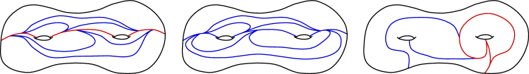
Figure 1: The three prototypical types of bending laminations are depicted by approximating train tracks. All of the mass of the affine bending measure is concentrated on the blue leaves, while the components of red leaves are orientable and accumulate non-trivial exponential growth/decay in one direction.

In Ungemach’s examples, reproduced here in the Appendix for convenience of the reader, a well-chosen isolated simple geodesic $\ell$ spirals onto a closed leaf with non-trivial holonomy. An element in $E^{\rho}_{2}|_{\ell}$ decays exponentially under parallel transport as it spirals. In particular, these vectors attached to the intersection of $\ell$ with a transverse arc $k$ crossing the simple closed curve are summable (using the flat connection on $E^{\rho}$). This is the first example of a flow invariant (Lemma 5.4) transverse measure valued in $E^{\rho}_{2}$ that encodes a non-trivial bending deformation along $\ell$. Locally, this is the tensor product of a flow equivariant transverse measure to $\lambda$ and a section of $E^{\rho}_{2}$ over the tangents to $\lambda$ (see §§4-5). The equivariance property required of the measure keeps track of the growth of vectors in $E^{\rho}_{2}$ along leaves of the geodesic foliation.

In order to get our hands on invariant transverse measures valued in $E^{\rho}_{2}|_{\lambda}$ more generally, we first construct flow invariant measures on $T^{1}X$ that are supported on the tangents to a geodesic lamination. For a minimal lamination $\lambda$ and point $p\in\widehat{\lambda}$ satisfying the hypothesis of Theorem 1.1, invariant measures are obtained as weak-$*$ limits of almost invariant measures on the unit tangent bundle supported on $\widehat{\lambda}$: for $v\in E_{2}^{\rho}|_{p}$, define

$$\frac{1}{N(t)}{\int_{-t}^{t}\left(g_{[0,s]}\right)_{*}v\cdot\delta_{g_{s}p}~{}ds},$$ (1)

where $N(t)$ is a normalizing factor ensuring sub-convergence.

We prove in §4 that any weak-$*$ accumulation point of (1) defines an invariant $E_{2}^{\rho}$-valued measure on $T^{1}X$. Without the non-positive exponential growth growth hypothesis along the $g_{t}$-orbit of $p$, sublimiting measures do not exhibit the required invariance. Pushing this down to the surface and integrating off the flow direction yields a transverse invariant $E^{\rho}_{2}$-valued measure and specifies a non-trivial bending deformation with support $\lambda$. Conversely, all bending data is of this form (§5).

Remark 1.3.

By choosing a point in the leaf space of the bending lamination and integrating the transverse $E^{\rho}_{2}$-valued bending measure, it is possible to obtain a description of one of the two dendrites at infinity in the maximal domain of discontinuity in the dual affine space.

A priori, a measure valued in a bundle need not admit any reasonable description, e.g., in terms of some finite combinatorial data. Miraculously, the bundles $E^{\rho}_{2}|_{\widehat{\lambda}}$ are flat, which in turn allows for a concise and manageable description of the transverse measures valued in $E^{\rho}_{2}$.

The antipodal involution on $T^{1}X$ induces a quotient $\overline{E}^{\rho}_{2}\to\mathbb{P}T^{1}X$ of $E^{\rho}_{2}\to T^{1}X$ (see §6). There is a natural embedding of $\lambda$ into $\mathbb{P}TX$ by taking tangents, so that $\overline{E}^{\rho}_{2}|_{\lambda}$ is defined by pullback. The transverse measure admits a pushforward to $\overline{E}^{\rho}_{2}|_{\lambda}$.

Theorem 1.4.

There is a Hölder continuous flat connection on $\overline{E}^{\rho}_{2}|_{\lambda}$ called the slithering connection. Its holonomy can be recorded as a representation

$$\chi:\pi_{1}\tau\to\mathbb{R}^{\times},$$

where $\tau$ is a snug train track carrying $\lambda$.

We make sense of a flat connection on a geodesic lamination extending a given connection along the leaves in §6, which is also where we construct the slithering connection from the slithering maps defined by Bonahon–Dreyer [BD17]. These maps provide local transverse trivializations of $\overline{E}^{\rho}_{2}|_{\lambda}$ on collections of fellow-travelling leaves, and the existence of the holonomy follows.

Because this bundle is flat, the invariant transverse measure valued in $\overline{E}^{\rho}_{2}|_{\lambda}$ factors nicely. It is a transverse measure, equivariant with respect to the holonomy $\chi$, tensored with a flat section over transversals. This is a more tractable object.

Corollary B.

The bending measure valued in $\overline{E}^{\rho}_{2}|_{\lambda}$ is affine (see §7 for definitions). Consequently,

• This measure may be written as a finite collection of positive real numbers on a train track with stops and holonomy $\chi$ given by Theorem 1.4,

• If $k$ is a suitable transversal to $\lambda$, then geodesic flow induces a first return map to $\widehat{k}\cap\widehat{\lambda}$, the tangents to $\lambda$ over $k$. Integrating the affine measure on $\widehat{k}\cap\widehat{\lambda}$ produces an affine interval exchange transformation (AIET) with flips and involutive symmetry that is measurably semi-conjugate to this first return system; see §7.2.

See also [HO92] for a discussion of affine measured laminations. We remark, however, that our flat line bundles are only defined over (a neighborhood of) the bending lamination, and this bundle does not in general extend to a flat line bundle over the whole surface (see equation (17)).

In §7, we define a space $\mathcal{ML}^{\rho}(S)$ of pairs consisting of flat line bundles over laminations with slithering connection determined by $\rho$ and affine measures valued in that bundle. There is a weak-$*$ topology on $\mathcal{ML}^{\rho}(S)$, described in §7.4.

An orientation on the surface $S$ and on the model space distinguish (globally) the ‘top’ and ‘bottom’ of the convex core boundary. As a result of the work we have outlined so far, there exists a natural map

$$\beta_{+}:\{\eta:\pi_{1}S\rightarrow\operatorname{Aff}^{*}(3,\mathbb{R})~{}\text{irreducible}\mid L(\eta)\in\operatorname{SL}(3,\mathbb{R}).\rho\}/\operatorname{Aff}^{*}(3,\mathbb{R})\to\mathcal{ML}^{\rho}(S)$$

recording the affine bending lamination on the top component of the convex hull $\Xi_{\eta}$ from a coaffine representation with linear part $\rho$.

Theorem C.

The map $\beta_{+}$ is a homeomorphism that is homogeneous with respect to positive scale. Consequently, the projectivization $\mathcal{PML}^{\rho}(S)$ is a sphere of dimension $6g-7$.

It would be interesting to understand how our work relates to the work of Seppi and Ni on surfaces of constant affine Gaussian curvature [NS22], as well as to the forthcoming work of Antoine Ablondi, who treats exactly the representations we examine here, but from the (dual) perspective of affine geometry.

We would be very interested to know what the typical behaviors for the bending data are. Via Corollary B, there are analogous (open) questions about AIETs with flips (and symmetry) and possible connections to half dilation surfaces (e.g., [Gha21, Wan19]). For example, we would like to know when our affine transverse measures are purely atomic (so that the corresponding AIET with flips has a wandering interval [GLP09, Cob02, MMY10]), which seems to be a dense and open condition, but perhaps not full measure. It would be interesting also to identify which pairs of affine laminations appear on the boundary of the convex core of a convex cocompact coaffine surface group action, extending what’s known at the Fuschian locus [Bon05].

1.2 Outline of the paper

Section 2 establishes notation, background, and the fundamental objects and structures of study. Notably, the basics of coaffine geometry are developed in §2.2, and §2.5 establishes notation for Anosov representations, including the flat bundles $F^{\rho}\to S$ and $E^{\rho}\to T^{1}S$, and the relationship between them.

Section 3 explores the data which may be extracted from a convex cocompact coaffine representation $\eta$ through purely geometric techniques. In particular, Lemma 3.19 defines the ‘macroscopic’ bending data for each boundary component of the minimal convex domain of discontinuity $\Xi_{\eta}$. For each component, we obtain a cocycle $\psi\in Z^{1}(S,F^{\rho})$ describing the bending, which is supported on a lamination $\lambda$, in the sense outlined in Lemma 3.19. The main technical and geometric results in this section are Corollaries 3.15 and 3.21, which show that the bending lies close to the line $E_{2}^{\rho}|_{\ell}$ when evaluated on arcs that shrink to a leaf $\ell$ of the bending lamination on $\partial\Xi_{\eta}$.

Section 4 defines the space $\mathcal{ML}(T^{1}X)^{G}$ of flow equivariant measures supported on the tangents to laminations in $T^{1}X$ and gives a dynamical characterization for when a geodesic lamination can support such a measure by attempting to build one. Theorems 1.1 and 1.2 are proved in §4.1. In §4.2, we define the space of equivariant transverse measures $\mathcal{ML}(X)^{G}$ and a disintegration map $\mathcal{ML}(T^{1}X)^{G}\to\mathcal{ML}(X)^{G}$ which we then prove is a homeomorphism (Proposition 4.17).

Section 5 builds on §4 by constructing cocycles from equivariant measures (§5.1) and extracting an equivariant transverse measure from a bending cocycle $\psi$ with support $\lambda$ (§5.2). The main result from this section is Theorem 5.1, which explicates the relationship between equivariant measures and cohomology through a homeomorphism, $\Phi:\mathcal{ML}(X)^{G}\to H^{1}(S,F^{\rho})\setminus\{0\}$.

Section 6 is independent from the previous sections and contains results that could be of separate utility. In §6.1 we develop a definition of flat connections over geodesic laminations extending a given connection along the leaves, and in §6.2 we show that the bundle $\overline{E}^{\rho}_{2}|_{\lambda}$ is flat by way of constructing the slithering connection. In this section we use $F^{\rho}_{2}\to\lambda$ to denote $E^{\rho}_{2}|_{\lambda}$.

The paper culminates in Section 7, where we prove our Main Theorems A and C as well as Corollary B. §7.1 places the measures in $\mathcal{ML}(X)^{G}$ in the context of affine measures, using the flat structure on $\overline{E}^{\rho}_{2}|_{\lambda}$ constructed in §6. Then, §7.2 makes precise how such an affine measure relates to an affine interval exchange transformation (AIET) with flips and §7.3 relates our notion of affine measured laminations with the notion studied by Hatcher and Oertel. §7.4 proves that $\beta_{+}$ is a homeomorphism (Theorem 7.16).

Finally, the Appendix is a motivating example. It is designed to be maximally independent from the rest of the paper, except the background material, and is intended to be readable by a proficient graduate student familiar with the basic context.

2 Preliminaries

2.1 Vector spaces

Throughout we will work with finite dimensional vector spaces and their dual spaces, often simultaneously. Recall that the general (and special) linear groups of a vector space $V$ act on the dual space $V^{*}$ by

$$A.\alpha=\alpha\circ A^{-1}$$

for $A\in\operatorname{GL}(V)$ and $\alpha\in V^{*}$. This action is natural: it is the unique action preserving the evaluation between $V$ and $V^{*}$, and required no additional data. For finite dimensional vector spaces, the groups $\operatorname{GL}(V)$ and $\operatorname{GL}(V^{*})$ are therefore naturally identified.

Given a representation $r:\Gamma\rightarrow\operatorname{GL}(V)$, there is thus an action of $\Gamma$ on both $V$ and $V^{*}$. We denote these vector spaces with their $\Gamma$-actions as $V_{r}$ and $(V^{*})_{r}$ respectively.

A choice of (ordered) basis $\{e_{1},\dots,e_{d}\}$ for a finite-dimensional vector space $V$ gives a standard choice of basis $\{e^{1},\dots,e^{d}\}$ for $V^{*}$ by the defining property $e^{i}(e_{j})=\delta^{i}_{j}$.

2.2 Coaffine geometry

Let $\operatorname{Aff}^{*}(3,\mathbb{R})<\operatorname{SL}(4,\mathbb{R})$ denote the group of coaffine transformations acting on $\operatorname{\mathbb{R}\textrm{P}}^{3}$. That is, $\operatorname{Aff}^{*}(3,\mathbb{R})$ is defined (up to conjugacy in $\operatorname{SL}(4,\mathbb{R})$) by

$$\operatorname{Aff}^{*}(3,\mathbb{R})=\left\{\begin{pmatrix}A&\mathbf{0}\\ \tau&1\end{pmatrix}\mid A\in\operatorname{SL}(3,\mathbb{R}),\tau\in\left(\mathbb{R}^{3}\right)^{*}\right\},$$

where $\mathbf{0}$ denotes the zero vector in $\mathbb{R}^{3}$. The coaffine group is the point stabilizer for the action of $\operatorname{SL}(4,\mathbb{R})$ on $\mathbb{R}^{4}$. In the parametrization used at present, this point is (any non-zero scalar multiple of) $e_{4}\in\mathbb{R}^{4}$. The coaffine space $\operatorname{\mathbb{R}\textrm{P}}^{3}\setminus\{[e_{4}]\}$ is a homogenous space for $\operatorname{Aff}^{*}(3,\mathbb{R})$.

Definition 2.1.

In the language of $(G,X)$-structures, $\operatorname{SL}(3,\mathbb{R})$-coaffine geometry (in this context, simply coaffine geometry), is the pair

$$\left(\operatorname{Aff}^{*}(3,\mathbb{R}),\operatorname{\mathbb{R}\textrm{P}}^{3}\setminus\{[e_{4}]\}\right).$$

There is a homomorphism $\operatorname{Aff}^{*}(3,\mathbb{R})\rightarrow\operatorname{SL}(3,\mathbb{R})$ which takes the matrix $A$ from the definition above; this is the linear part of an element of $\operatorname{Aff}^{*}(3,\mathbb{R})$. We will say that an element $T\in\operatorname{Aff}^{*}(3,\mathbb{R})$ with trivial linear part is a translation, and let $\operatorname{TAff}^{*}(3,\mathbb{R})$ be the normal subgroup of translations; it is a $3$-dimensional vector space. There is a short exact sequence

$$1\to\operatorname{TAff}^{*}(3,\mathbb{R})\to\operatorname{Aff}^{*}(3,\mathbb{R})\to\operatorname{SL}(3,\mathbb{R})\to 1,$$

which splits, so that

$$\operatorname{Aff}^{*}(3,\mathbb{R})\cong\operatorname{TAff}^{*}(3,\mathbb{R})\rtimes\operatorname{SL}(3,\mathbb{R}).$$

Then $\operatorname{SL}(3,\mathbb{R})$ acts naturally on $\operatorname{TAff}^{*}(3,\mathbb{R})$ by conjugation.

The point $[e_{4}]\in\operatorname{\mathbb{R}\textrm{P}}^{3}$ defines a hyperplane in the dual projective space:

$$[\ker e_{4}]=\left\{[\alpha]\in\left(\operatorname{\mathbb{R}\textrm{P}}^{3}\right)^{*}:\alpha(e_{4})=0\right\}.$$

Denote by

$$\left(\mathbb{A}^{3}\right)^{*}=\left(\operatorname{\mathbb{R}\textrm{P}}^{3}\right)^{*}\setminus[\ker e_{4}],$$

accompanied by the action by $\operatorname{Aff}^{*}(3,\mathbb{R})$, which preserves $\left(\mathbb{A}^{3}\right)^{*}\subset(\operatorname{\mathbb{R}\textrm{P}}^{3})^{*}$. It is isomorphic to the usual $3$-dimensional affine space $\operatorname{\mathbb{A}}^{3}$, i.e., the set of hyperplanes in $\operatorname{\mathbb{R}\textrm{P}}^{3}$ which do not intersect $[e_{4}]$ form a copy of the $\operatorname{SL}(3,\mathbb{R})$-affine space under the action of $\operatorname{Aff}^{*}(3,\mathbb{R})$.

Let us choose the vector $e_{4}\in\mathbb{R}^{4}$ as a representative of its projective class, and consider the affine chart for $\left(\mathbb{A}^{3}\right)^{*}$ given by

$$\left\{\alpha\in\left(\mathbb{R}^{4}\right)^{*}:\alpha(e_{4})=1\right\}.$$

Abusing notation, we write $\alpha\in\left(\mathbb{A}^{3}\right)^{*}$ to mean that $\alpha(e_{4})=1$ (and therefore $[\alpha]\in(\operatorname{\mathbb{A}}^{3})^{*}$).

For $\alpha,\beta\in\left(\mathbb{A}^{3}\right)^{*}$, we have $(\alpha-\beta)\in\ker e_{4}\cong(\mathbb{R}^{3})^{*}$. We may thus view $\ker e_{4}$ as the (normal) subgroup of translations in $\operatorname{Aff}^{*}(3,\mathbb{R})$ by

$$\tau\in\ker e_{4}\mapsto\begin{pmatrix}I_{3}&\mathbf{0}\\ \tau&1\end{pmatrix}.$$

For any $\delta\in\mathbb{R}\setminus\{0\}$, the affine chart

$$\left\{\alpha\in\left(\mathbb{R}^{4}\right)^{*}:\alpha(e_{4})=\delta\right\}$$

effects our identification of the translation subgroup of $\operatorname{Aff}^{*}(3,\mathbb{R})$ via conjugation by

$$\begin{pmatrix}\delta^{-1/3}I_{3}&\\ &\delta\end{pmatrix}\in\operatorname{SL}(4,\mathbb{R}).$$

Remark 2.2.

Any equivariant identification between $\operatorname{TAff}^{*}(3,\mathbb{R})$ and $(\mathbb{R}^{3})^{*}$ requires a choice. However, we will frequently use ‘$(\mathbb{R}^{3})^{*}$’ as shorthand notation for $\operatorname{TAff}^{*}(3,\mathbb{R})$, and ‘$(\operatorname{\mathbb{R}\textrm{P}}^{2})^{*}$’ for $\mathbb{P}\operatorname{TAff}^{*}(3,\mathbb{R})$.

Example 2.3.

To understand the geometric meaning of a translation on the coaffine space, let us use coordinates. For any pair $\alpha\not=\beta\in(\operatorname{\mathbb{A}}^{3})^{*}$, the kernels $[\ker\alpha]$ and $[\ker\beta]$ intersect in a projective line $L\subset\operatorname{\mathbb{R}\textrm{P}}^{3}$ which itself does not contain $[e_{4}]$. See Figure 2

Choose a pair of distinct vectors $e_{1}$ and $e_{3}$ with projective classes in $L$ as two vectors of a basis, and let $e_{2}$ be any vector so that $[e_{2}]\in[\ker\alpha]\setminus L$. In these coordinates, the unique translation taking $\alpha$ to $\beta$ is

$$Z_{t}=\begin{pmatrix}I_{3}&\mathbf{0}\\ te^{2}&1\end{pmatrix}\in\operatorname{Aff}^{*}(3,\mathbb{R}),$$

for some particular $t$. Note also that $\beta-\alpha=te^{2}.$ From a coordinate-free perspective and using the identification of $\mathbb{P}\operatorname{TAff}^{*}(3,\mathbb{R})\cong[\ker e_{4}]$, we have that $[\beta-\alpha]\in[\ker L]\subset[\ker e_{4}]$.

Conversely, every non-trivial translation $\tau\in\operatorname{Aff}^{*}(3,\mathbb{R})$ preserves a unique line $L_{\tau}\subset\operatorname{\mathbb{R}\textrm{P}}^{3}$ which does not intersect $[e_{4}]$.

Consider a positive diagonal element $A\in\operatorname{Aff}^{*}(3,\mathbb{R})<\operatorname{SL}(4,\mathbb{R})$, which in the present coordinates preserves the line $L$. Observe (by computation) that the centralizer of $A$ in $\operatorname{Aff}^{*}(3,\mathbb{R})$ contains no translation when the linear part of $A$ has eigenvalues all distinct from $1$ (except, necessarily, the eigenvalue of $e_{4}$). Suppose that the second eigenvalue of $A$ were equal to $1$. Then the centralizer of $A$ contains the subgroup $\{Z_{t}\}$. This will be relevant later for the deformation theory of coaffine representations of surface groups.

2.3 Surfaces and geodesic laminations

The reader looking for an introduction to surface theory and geodesic laminations is advised to consult [Thu22, CB88, PH92, ZB04].

2.3.1 Negatively curved metrics and flows

Let $S$ be a closed oriented surface of genus $g$ at least $2$, and let $X$ denote the data of $S$ equipped with a negatively curved Riemannian metric. Let $T^{1}X$ be the unit tangent bundle and let

$$g_{t}:T^{1}X\to T^{1}X$$

be the time $t$ map for the geodesic flow. The Levi-Civita connection on $X$ gives us a way to lift the Riemannian metric on $X$ to one on $T^{1}X$.

Denote by $\partial\widetilde{X}$ the visual boundary of the universal cover $\widetilde{X}$ of $X$. Given a point $x\in\widetilde{X}$, the exponential map induces a homeomorphsim $T^{1}_{x}X\cong\partial\widetilde{X}$. The angular metric on $T^{1}_{x}X$ gives $\partial\widetilde{X}$ a metric, where the identity map on $\partial\widetilde{X}$ is a bi-Lipschitz equivalence for the angular/visual metrics for points $x,y\in X$.

Negative curvature gives that for any pair $z,w\in\partial\widetilde{X}$ of distinct points there is a unique geodesic line from $z$ to $w$. The space of geodesic lines is the quotient of $\partial\widetilde{X}\times\partial\widetilde{X}\setminus\Delta$ by the order two symmetry swapping the future for the past, where $\Delta$ denotes the diagonal. Then the family of angular metrics on $X$ gives the space of geodesics a bi-Lipschitz class of metrics.

Suppose $Y$ is another metric on $S$ such that $\widetilde{Y}$ is a uniquely geodesic visibility space and that the identity map $X\to Y$ is a bi-Lipschitz equivalence. For example, $Y$ is another negatively curved metric or the Hilbert metric for a properly convex projective structure (see §2.4). The Gromov product can be used to define a Hölder class of metrics on $\partial\widetilde{Y}$.

The identity map lifts to a quasi-isometry of universal covers and extends to a bi-Hölder continuous map between $\partial X\cong\partial Y$. Thus the spaces of (un)oriented geodesic lines in $X$ and in $Y$ have a well defined bi-Hölder class of metrics. There is also a bi-Hölder continuous

$$\varphi:T^{1}X\to T^{1}Y$$ (2)

orbit equivalence between the two geodesic flows [KH95, §19.1].

2.3.2 Geodesic laminations

A geodesic lamination $\lambda$ on $X$ is a closed subset of $X$ equipped with a foliation by complete geodesics, called its leaves. A geodesic lamination $\lambda$ is orientable if its leaves can be continuously oriented. Every lamination $\lambda$ has a two-fold orientation cover $\widehat{\lambda}\to\lambda$, where $\widehat{\lambda}$ is an orientable lamination. The set of tangents $T^{1}\lambda\subset T^{1}X$ is naturally identified with $\widehat{\lambda}$.

Examples of geodesic laminations are furnished by disjoint unions of simple, closed geodesics on $X$ and the full preimages of such in $\widetilde{X}$. Any family of disjoint complete geodesic lines in $\widetilde{X}$ that is invariant under the action of $\pi_{1}S$ by deck transformations descends to a geodesic lamination. Using the boundary map $\widetilde{X}\cong\widetilde{Y}$, we therefore obtain a bijective correspondence between the geodesic laminations on $X$ and the geodesic laminations on $Y$.

A geodesic lamination $\lambda$ is minimal if every (half-)leaf is dense in $\lambda$. If $\lambda$ is minimal and has an infinite leaf, then the transversal space is a cantor set. Generally, $\lambda\subset X$ decomposes as a union of at most $3g-3$ minimal sublaminations and at most $6g-g$ many infinite isolated leaves that spiral onto the minimal components. We say that $\lambda$ is maximal if it is not contained in any other geodesic lamination on $X$. Every geodesic lamination is contained in a maximal geodesic lamination, called a maximal completion.

The projective tangent bundle $\mathbb{P}TX$ is the quotient of $T^{1}X$ by the fiberwise antipodal involution and caries a metric making the quotient map a local isometry. Every geodesic lamination $\lambda\subset X$ can be embedded in $\mathbb{P}TX$ as its tangent line field $\mathbb{P}T\lambda$. The following lemma can be deduced from [Ker83, Lemma 1.1].

Lemma 2.4.

The map $x\in\lambda\mapsto[T_{x}\lambda]\in\mathbb{P}T\lambda$ is a bi-Lipschitz homeomorphism.

There is a Hausdorff metric $d_{X}^{H}$ on the set of geodesic laminations coming from the restriction of the Hausdorff metric on closed subsets of $X$. This metric gives the set of geodesic laminations the structure of a compact metric space. While the orbit equivalence from (2) need not induce a Hölder map $\mathbb{P}TX\to\mathbb{P}TY$, it does however induce a Hölder map between closed invariant sets of the geodesic foliations of $\mathbb{P}TX$ and $\mathbb{P}TY$ with their Hausdorff metrics. Thus, Lemma 2.4 together with (2) show that the Hausdorff metric on geodesic laminations depends bi-Hölder continuously on $X$ (see also [ZB04, Lemma 7]).

Let $\epsilon>0$ be given, and consider the $\epsilon$-neighborhood $\mathcal{N}_{\epsilon}(\lambda)\subset X$. For $\epsilon$ small enough, this neighborhood can be foliated by contractible $C^{1}$ arcs called ties that meet $\lambda$ transversely, for example using Thurston’s horocycle foliation [Thu22, Thu98] or the construction of the orthogeodesic foliation studied in [CF23, CF24]. Such a foliated neighborhood is called a train track neighborhood.

If every component of $X\setminus\mathcal{\mathcal{N}}$ is a deformation retract of the component of $X\setminus\lambda$ containing it, then we say that $\mathcal{N}$ is a snug for $\lambda$. If $\epsilon$ is small enough, then $\mathcal{N}$ is snug for $\lambda$. A snug neighborhood $\mathcal{N}$ has the property that if $k$ is a tie, and $J$ is a complementary component of $k\setminus\lambda$ not containing an endpoint of $k$, then the leaves corresponding to the endpoints of $J$ are asymptotic in $\lambda$; this can be proved directly from the definition of snugness. The orientation covering $\widehat{\lambda}\to\lambda$ extends to a two-fold covering $\widehat{\mathcal{N}}\to\mathcal{N}$ if $\mathcal{N}$ is snug.

The leaf space of the foliation of $\mathcal{N}=\mathcal{N}_{\epsilon}(\lambda)$ by ties, denoted by $\tau$, has the structure of a train track, i.e., a graph with a $C^{1}$ structure at its vertices (called switches) and edges (called branches) satsifying a number of non-degeneracy conditions that can be $C^{1}$-embedded in $\mathcal{N}$ transverse to the ties. See [PH92, §1.1] or [Thu22, §8.9].

For topological reasons, the $2$-dimensional Lebesgue measure of a geodesic lamination on a closed surface is zero. For a $C^{1}$ arc $k$ transverse to $\lambda$, Fubini then implies that the $1$-dimensional Lebesgue measure of $k\cap\lambda$ is zero. A proof of the following lemma can be adapted from [Far23, Proposition 4.1] or from the arguments in [Bon96, §1]. The lemma implies also that the Hausdorff dimension of $\lambda$ is $1$; see also [BS85].

Lemma 2.5.

For any given $C^{1}$ arc $k$ transverse to $\lambda\subset X$ and $\epsilon>0$, the connected components of $k\cap\mathcal{N}_{\epsilon}(\lambda)$ each have diameter $O(\epsilon)$, and there are at most $O(\log 1/\epsilon)$ such components.

A transversely measured geodesic lamination $\mu$ with support $\lambda$ is the assignment of, for every arc $k$ transverse to $\lambda$, a finite positive Borel measure $\mu_{k}$ with support equal to $\lambda\cap k$. The assignment $k\mapsto\mu_{k}$ is required to be natural under restriction and to be slide invariant, i.e., if $k^{\prime}$ is homotopic via $H$ to $k$ through arcs transverse to $\lambda$, then $H_{*}\mu_{k}=\mu_{k^{\prime}}$. If $\lambda$ has isolated leaves, then it is not the support of a transverse measure. Thurston’s space $\mathcal{ML}(S)$ of measured geodesic laminations is a manifold whose positive projectivization $\mathcal{PML}(S)$ is a sphere of dimension $6g-7$ [Thu88]. Thurston constructed a natural measure (called the Thurston measure) on $\mathcal{ML}(S)$ in the class of Lebesgue.

A minimal geodesic lamination $\lambda$ is called uniquely ergodic if the simplex of measures in $\mathcal{ML}(S)$ whose support is $\lambda$ is a ray. For the Thurston measure, the support of almost every measured lamination is maximal, minimal, non-orientable, and uniquely ergodic [Ker85].

2.4 Hitchin representations and convex $\operatorname{\mathbb{R}\textrm{P}}^{2}$-geometry

We require some general facts about the Hitchin component of surface group representations into $(\mathrm{P})\operatorname{SL}(3,\mathbb{R})$, and the geometry of convex projective structures on the surface $S$. For the uninitiated, there are two helpful surveys on convex projective structures, one by Choi, Lee, and Marquis [CLM18] and one by Benoist [Ben08].

A subset of the real projective space $\operatorname{\mathbb{R}\textrm{P}}^{d}$ is properly convex if its closure is contained in an affine chart and it is convex in such a chart. A (real, properly) convex projective structure on a surface $S$ is an (incomplete) $(\operatorname{SL}(3,\mathbb{R}),\operatorname{\mathbb{R}\textrm{P}}^{2})$-structure so that the developing map is a homeomorphism to some open properly convex subset $\Omega\subset\operatorname{\mathbb{R}\textrm{P}}^{2}$.

Goldman and Choi demonstrated that the set of holonomies (considered up to conjugacy) of convex projective structures on a surface form a component of the $\operatorname{SL}(3,\mathbb{R})$-character variety. This component is usually called the Hitchin comonent and is denoted $\operatorname{Hit}_{3}$ [CG93, Lab06].

A hyperbolic structure on a surface is therefore an example of a convex projective structure: the developing map of such a structure is a homeomorphism to $\operatorname{\mathbb{H}}^{2}$, which may be realized as the projective (Klein) model. This is a properly convex domain in $\operatorname{\mathbb{R}\textrm{P}}^{2}$. Any properly convex domain is a metric space with the Hilbert metric; the projective lines are geodesics for this metric.

In general, for a representation $\rho$ with $[\rho]\in\operatorname{Hit}_{3}$, the domain $\Omega=\Omega(\rho)$ is strictly convex and the boundary $\partial\Omega$ has regularity $C^{1+a}$ for some $a\in(0,1]$ [Ben04]. It is true in general that if a domain $\Omega$ is $C^{1}$ and strictly convex, then $\Omega^{*}$ is as well.

As in the case of hyperbolic geometry, there is a $(\pi_{1}S,\rho)$-equivariant Hölder-continuous identification

$$\xi=\xi(\rho):\partial\pi_{1}S\to\partial\Omega\subset\operatorname{\mathbb{R}\textrm{P}}^{2}.$$ (3)

In the dual projective space $(\operatorname{\mathbb{R}\textrm{P}}^{2})^{*}$, the action of $\rho$ preserves a convex projective domain $\Omega^{*}$, which is described as

$$\Omega^{*}=\{[\alpha]\in(\operatorname{\mathbb{R}\textrm{P}}^{2})^{*}\mid[\ker\alpha]\cap\overline{\Omega}=\emptyset\}.$$

It is not difficult to check that $\Omega^{*}$ is a properly convex projective domain, and so also is furnished with a limit map

$$\xi^{*}=\xi^{*}(\rho):\partial\pi_{1}S\to\partial\Omega^{*}\subset(\operatorname{\mathbb{R}\textrm{P}}^{2})^{*}.$$

The maps $\xi$ and $\xi^{*}$ have the property that for all $z\in\partial\pi_{1}S$, $\xi^{*}(z)(\xi(z))=0$, i.e., the hyperplane $\xi^{*}(z)$ is the unique supporting hyperplane to $\Omega$ at the point $\xi(z)$.

2.5 The Anosov property

We require some of the theory of Anosov representations from a closed surface group into $\operatorname{SL}(d,\mathbb{R})$ following Labourie [Lab06]. For further development of the theory of Anosov representations, see [GW12, BPS19, KLP17].

Let $\rho:\pi_{1}S\to\operatorname{SL}(d,\mathbb{R})$ be a representation. We construct a flat $(\mathbb{R}^{d})^{*}$-bundle over $S$ by pushing forward the flat connection on the trivial bundle $\widetilde{S}\times(\mathbb{R}^{d})^{*}$ to the quotient by the diagonal action:

$$F^{\rho}=\left(\widetilde{S}\times(\mathbb{R}^{d})^{*}\right)/\left[(x,v)\sim(\gamma.x,\rho(\gamma)v)\right].$$

The flat connection on $F^{\rho}$ is called $\nabla^{\rho}$.

Choose for reference a hyperbolic metric $X$ on $S$ and a continuously varying inner product on $F^{\rho}$, and consider the flat bundle $E^{\rho}\to T^{1}X$ obtained by pulling back $F^{\rho}$ along the projection $\pi:T^{1}X\to X\cong S$. By abuse of notation, we denote also the flat connection on $E^{\rho}$ by $\nabla^{\rho}$. To define the Anosov property, we consider the parallel transport along flow lines for the geodesic flow.

Definition 2.6.

We say that $\rho$ is Anosov if there are constants $c_{1},c_{2}>0$ a Hölder continuous splitting $E^{\rho}_{1}\oplus...\oplus E^{\rho}_{k}$ of $E^{\rho}$ such that for $i<j$ we have

$$\frac{\|\left(g_{[0,t]}\right)_{*}v_{i}\|}{\|\left(g_{[0,t]}\right)_{*}v_{j}\|}\leq c_{2}e^{-c_{1}t},$$

for all $t\geq 0$ and unit vectors $v_{i}\in E_{i}^{\rho}$ and $v_{j}\in E_{j}^{\rho}$, where $\left(g_{[0,t]}\right)_{*}$ is the parallel transport along the segment $g_{[0,t]}$. When $k=d$, $\rho$ is Borel-Anosov. When $\dim E^{\rho}_{1}=1$, $\rho$ is projective-Anosov.

There is an analogously defined bundle $(E^{\rho})^{*}$ constructed from the natural action of $\rho$ on $\mathbb{R}^{d}$. Its Anosov-splitting is dual to the Anosov splitting of $(E^{\rho})^{*}$ for dynamical reasons.

The antipodal involution $p\mapsto\overline{p}$ satisfies $g_{t}\overline{p}=\overline{g_{-t}p}$, and so induces a symmetry

$$E^{\rho}_{i}|_{p}=E^{\rho}_{k-i}|_{\overline{p}},$$

so that the dimensions of the factors in the splitting match up in pairs: $\dim E^{\rho}_{i}=\dim E^{\rho}_{k-i+1}$.

Remark 2.7.

Anticipating what is to come in §4, we point out that if $v\in E^{\rho}$ satisfies

$$\limsup_{t\to\infty}\frac{1}{t}\log\left\|\left(g_{[0,t]}\right)_{*}v\right\|=0,$$

then $k$ is odd, and $v\in E_{(k+1)/2}$.

Because the splitting $(E^{\rho})^{*}=(E^{\rho}_{1})^{*}\oplus\dots\oplus(E^{\rho}_{k})^{*}$ is $g_{t}$-invariant, it provides a limit curve with image in $\operatorname{\mathbb{R}\textrm{P}}^{d-1}$ when $\rho$ is projective- (or Borel-) Anosov:

$$\xi:\partial\pi_{1}S\rightarrow\operatorname{\mathbb{R}\textrm{P}}^{d-1},$$

by assigning to $z\in\partial\pi_{1}S$ the projective class of $(E^{\rho})^{*}_{k}|_{p}$ for any $p\in T^{1}X$ satisfying $\lim_{t\rightarrow\infty}(g_{t}p)=z$.

The map $\xi$ is $\rho$-equivariant, and is the same curve from Equation (3) in the case that $[\rho]\in\operatorname{Hit}_{3}$.

We will take a special interest in the bundle $E^{\rho}_{2}$ for $[\rho]\in\operatorname{Hit}_{3}$. The following lemma will be helpful in the constructions of Section 4.

Lemma 2.8.

Let $\rho:\pi_{1}S\to\operatorname{SL}(3,\mathbb{R})$ be so that $[\rho]\in\operatorname{Hit}_{3}$, and let $E^{\rho}=E^{\rho}_{1}\oplus E^{\rho}_{2}\oplus E^{\rho}_{3}$ be the Anosov splitting of the associated flat bundle. Then the line-bundle $E^{\rho}_{2}$ admits a global Hölder continuous (non-zero) section.

Proof.

Because this is a topological statement, it is sufficient (by the Thurston-Ehrasmann principle) to complete the proof in the case that $\rho$ is Fuchsian: when $\rho(\pi_{1}S)<\operatorname{\mathbb{SO}}(2,1)<\operatorname{SL}(3,\mathbb{R}).$

Since the image of the holonomy is in the special linear group, the bundle $E^{\rho}$ is orientable (i.e. the associated orientation bundle admits a global section). Every Fuchsian representation in $\operatorname{Hit}_{3}$ not only lies in $\operatorname{\mathbb{SO}}(2,1)$, but also in the identity component: $\operatorname{\mathbb{SO}}_{\circ}(2,1)$. The group $\operatorname{\mathbb{SO}}(2,1)$ preserves a quadratic form $Q$ of signature $(2,1)$, and so preserves the set of null vectors for this form: $Z(Q)\subset\mathbb{R}^{3}$, which is a cone on a circle. The identity component $\operatorname{\mathbb{SO}}_{\circ}(2,1)$ may be defined by the property that it preserves the two components of $Z(Q)\setminus\{0\}$. As a result, there exists a global continuously varying choice of component of this cone in $\mathscr{C}\subset E^{\rho}\cong(E^{\rho})^{*}$ where the bundles are identified by $Q$.

The limit curve $\xi$ in the Fuchsian case has image in the projectivization of $Z(Q)$. Upon making a choice of $\pm\mathscr{C}$, one has chosen a global orientation for the line-bundles $E^{\rho}_{1}$ and $E^{\rho}_{3}$: choose the direction that lies in $\mathscr{C}$. Call these sections $[x]$ and $[z]$ respectively. These orientations, in the presence of an orientation $o$ on $E^{\rho}$, co-orient $E^{\rho}_{2}$, by insisting that an orientation $[y]$ on $E^{\rho}_{2}$ satisfy

$$[x\wedge y\wedge z]=o$$

at every point. The regularity statement follows from the regularity of $\xi$; the lemma is proven. ∎

2.6 Cohomology with coefficients

Our primary reference for this material is [JM87]. Let $\Gamma$ be a group and $M$ be a connected CW-complex with fundamental group isomorphic to $\Gamma$, let $V$ be a vector space, and let $\rho:\Gamma\to\operatorname{GL}(V)$ be a representation. The cohomology of $\Gamma$ with coefficient module $V$ equipped with its $\rho$-action appears, e.g., when studying the space of (infinitesimal) deformations of $G$-conjugacy classes of representations of $\Gamma$ into a Lie group $G$; in this case, $V$ is the Lie algebra $\mathfrak{g}$ and $\rho$ is the adjoint representation of some $\eta:\Gamma\to G$.

We will only be interested in the $1$-dimensional cohomology defined as follows. The $1$-cocycles, denoted $Z^{1}(\Gamma,V_{\rho})$ are functions $\varphi:\Gamma\to V$ satisfying the cocycle relation

$$\varphi(\alpha\beta)=\varphi(\alpha)+\rho(\alpha)\varphi(\beta),~{}\forall\alpha,\beta\in\Gamma.$$

The coboundaries $B^{1}(\Gamma,V_{\rho})\leq Z^{1}(\Gamma,V_{\rho})$ are cocycles $\varphi$ for which there exist some $v\in V$ satisfying

$$\varphi(\gamma)=\rho(\gamma)v-v,~{}\forall\gamma\in\Gamma.$$

The cohomology $H^{1}(\Gamma,V_{\rho})$ is the vector space quotient of cocycles by coboundaries.

Let $\widetilde{M}$ be the universal cover of $M$. There is a flat $V$-bundle $F^{\rho}\to M$ constructed by pushing forward the (trivial) flat connection on $\widetilde{M}\times V$ to the quotient by the diagonal action:

$$F^{\rho}=(\widetilde{M}\times V)/[(x,v)\sim(\gamma.x,\rho(\gamma)v)].$$

Now we discuss the cohomology of $M$ with coefficients in $F^{\rho}$. Denote by $[0,1,2]$ the standard oriented $2$-simplex, so that, algebraically, we have

$$\partial[0,1,2]=[1,2]-[0,2]+[0,1].$$

The $1$-cochains $\psi$ assign to each singular $1$-simplex $\sigma:[0,1]\to M$ an element $\psi(\sigma)$ in the fiber of $F^{\rho}$ over $\sigma(0)$. A $1$-cochain $\psi$ is a cocycle if for every singular $2$-simplex $\tau:[0,1,2]\to M$, we have

$$\psi(\tau|_{[0,2]})=\psi(\tau|_{[0,1]})+\overline{\left(\tau|_{[0,1]}\right)}_{*}\psi(\tau|_{[1,2]}),$$

where $\overline{\left(\tau|_{[0,1]}\right)}_{*}:F^{\rho}|_{\tau(1)}\to F^{\rho}|_{\tau(0)}$ is the parallel transport. We say that $\psi$ is a $1$-coboundary if there is a (set theoretic) section $s:M\to F^{\rho}$ such that

$$\psi(\sigma)=\overline{\sigma}_{*}s(\sigma(1))-s(\sigma(0))$$

for all singular $1$-simplices $\sigma:[0,1]\to M$. The space of cocycles is denoted by $Z^{1}(M,F^{\rho})$ and the subspace of coboundaries is $B^{1}(M,F^{\rho})$. The cohomology $H^{1}(M,F^{\rho})$ is the vector space quotient of cocycles by coboundaries.

An identification of $\Gamma$ with $\pi_{1}(M,p)$ determines an isomorphism

$$H^{1}(M,F^{\rho})\to H^{1}(\Gamma,V_{\rho})$$ (4)

by evaluating cocycles only on loops based at $p$.

3 Coaffine geometry and convex cocompact representations

In this section, we study convex cocompact representations $\eta:\pi_{1}S\to\operatorname{Aff}^{*}(3,\mathbb{R})$ and show that the linear part $L(\eta)=\rho$ is Hitchin (Lemma 3.1). The converse, that every coaffine representation with Hitchin linear part acts convex cocompactly, is Lemma 3.7. The primary geometric object associated to these representations is their minimal convex domain of discontinuity, introduced in §3.2.

The main result of this section is that the boundary of this minimal domain hosts a pair of geodesic laminations on the underlying surface $S$ (Lemma 3.16) and that there exist macroscopic bending data which is transverse to these laminations (Lemma 3.20); the values that the bending cocycle attains are quantitatively close in a dual projective plane to the dual of the lamination (Corollary 3.21).

3.1 Coaffine Hitchin representations

We begin by showing that every convex cocompact coaffine representations acting on $\operatorname{\mathbb{R}\textrm{P}}^{3}$ has Hitchin linear part. There is a natural projection $Q:\mathbb{R}^{4}\rightarrow\mathbb{R}^{4}/[e_{4}]$, inducing a map

$$[Q]:\operatorname{\mathbb{R}\textrm{P}}^{3}\setminus\{[e_{4}]\}\rightarrow\mathbb{P}(\mathbb{R}^{4}/[e_{4}])\cong\operatorname{\mathbb{R}\textrm{P}}^{2}.$$ (5)

The map $Q$ is equivariant with respect to taking the linear part of a transformation $A\in\operatorname{Aff}^{*}(3,\mathbb{R})$, i.e.

$$L(A)\circ Q=Q\circ A.$$

Dual to $Q$, there is an inclusion $Q^{*}:\operatorname{TAff}^{*}(3,\mathbb{R})\cong\ker e_{4}\hookrightarrow\left(\mathbb{R}^{4}\right)^{*}$, inducing

$$[Q^{*}]:\mathbb{P}\operatorname{TAff}^{*}(3,\mathbb{R})\cong\left(\operatorname{\mathbb{R}\textrm{P}}^{2}\right)^{*}\hookrightarrow\left(\operatorname{\mathbb{R}\textrm{P}}^{3}\right)^{*}.$$

The action of $\operatorname{Aff}^{*}(3,\mathbb{R})$ preserves $\mathbb{P}\operatorname{TAff}^{*}(3,\mathbb{R})$.

Lemma 3.1.

Suppose $\eta:\pi_{1}S\to\operatorname{Aff}^{*}(3,\mathbb{R})$ is faithful and acts convex cocompactly on $\operatorname{\mathbb{R}\textrm{P}}^{3}$. Then the linear part $\rho=L(\eta)$ is Hitchin.

Proof.

Since $\eta$ is faithful, acts convex cocompactly, and $\pi_{1}S$ is hyperbolic, $\eta$ is projective-Anosov [DGK23]. The point $[e_{4}]$ cannot be in the image of the Anosov limit map $\xi$, as $\xi$ is equivariant and dynamics preserving. Indeed, if $[e_{4}]$ were in $\operatorname{im}\xi$, the action of $\pi_{1}S$ on $\partial\pi_{1}S$ would have a global fixed point, which would be a contradiction.

By assumption, the action of $\eta$ on the minimal convex domain

$$\Xi=\left(\operatorname{hull}\operatorname{im}\xi\right)\setminus\operatorname{im}\xi$$

is proper, so $\Xi$ also does not contain the point $[e_{4}]$. As a result, there exist a hyperplane $\alpha\subset\operatorname{\mathbb{R}\textrm{P}}^{3}$ separating $[e_{4}]$ and $\Xi$.

The action of $\eta$ on $(\mathbb{R}^{4}/[e_{4}])$ induced by the quotient $Q$ is $\rho=L(\eta)$. The representation $\rho$ is discrete and faithful for the following reason. If an infinite sequence of group elements $\gamma_{n}\in\pi_{1}S$ existed so that $\lim_{n\to\infty}\rho(\gamma_{n})=I$, then the translation part of $\eta(\gamma_{n})$ tends to infinity, as $\eta$ is discrete. In this case, the orbit of any point $x\in\Xi$ tends to $[e_{4}]$ under $\eta(\gamma_{n})$, contradicting the fact that $\Xi$ is invariant and bounded away from $[e_{4}]$. This shows that $\rho$ is discrete, and because $\pi_{1}S$ has no finite normal subgroups, $\rho$ is faithful by the same argument.

Since $\rho$ is discrete, faithful, and preserves an open proper convex projective domain

$$\Omega=[Q](\Xi)\subset\operatorname{\mathbb{R}\textrm{P}}^{2},$$

the quotient is homeomorphic to $S$. This is a properly convex projective structure on $S$, and thus $\rho$ is Hitchin by [CG93]. ∎

To reiterate, since $\rho$ is Hitchin, it preserves a properly convex $C^{1}$ and strictly convex projective domain

$$\Omega\subset\mathbb{P}(\mathbb{R}^{4}/[e_{4}])$$

and its dual action preserves the dual properly convex $C^{1}$ and strictly convex domain

$$\Omega^{*}\subset\mathbb{P}\operatorname{TAff}^{*}(3,\mathbb{R}).$$

In light of Lemma 3.1, we turn our attention to representations of the following prescribed form. Recall from Remark 2.2 that $(\mathbb{R}^{3})^{*}$ means $\operatorname{TAff}^{*}(3,\mathbb{R})$.

Definition 3.2.

Let $\rho:\pi_{1}S\rightarrow\operatorname{SL}(3,\mathbb{R})$ be a Hitchin representation, and let $\varphi\in Z^{1}(\pi_{1}S,(\mathbb{R}^{3})^{*}_{\rho})$. Define $\eta=\eta_{\varphi}:\pi_{1}S\rightarrow\operatorname{Aff}^{*}(3,\mathbb{R})$ by

$$\eta(\gamma)=\begin{pmatrix}\rho(\gamma)&\mathbf{0}\\ \varphi(\gamma^{-1})&1\end{pmatrix}.$$ (6)

Then $\eta$ is a coaffine representation with Hitchin linear part.

One checks that this is a representation using the cocycle condition; Lemma 3.1 states that all convex cocompact coaffine representations are of this form.

There is a relationship between reducible representations and coboundaries in this setting. Recall from §2.2 that

$$(\operatorname{\mathbb{A}}^{3})^{*}=\{[\alpha]\in(\operatorname{\mathbb{R}\textrm{P}}^{3})^{*}\mid\alpha(e_{4})=1\}.$$

When $\rho$ is reducible and of the form in (6), it preserves a hyperplane $[\ker\alpha]$ for some $\alpha\in\left(\mathbb{A}^{3}\right)^{*}$. Call such a representation $\eta_{\alpha}$. Conversely, every hyperplane $[\ker\alpha]$ which does not contain $[e_{4}]$ defines a linear section of the quotient $\mathbb{R}^{4}\rightarrow\mathbb{R}^{4}/[e_{4}]$, and an accompanying reducible representation $\eta_{\alpha}$ preserving this hyperplane. Note that the natural projection $\mathbb{R}^{4}\rightarrow\mathbb{R}^{4}/[e_{4}]$ restricted to $[\ker\alpha]$ is a linear isomorphism conjugating $\eta_{\alpha}$ to $\rho$.

For any pair of reducible representations $\eta_{\alpha}$ and $\eta_{\beta}$, the difference $\tau_{\beta\alpha}=\beta-\alpha\in\ker e_{4}$ is an element of the translation subgroup of $\operatorname{Aff}^{*}(3,\mathbb{R})$, and

$$\tau_{\beta\alpha}\eta_{\alpha}(\tau_{\beta\alpha})^{-1}=\eta_{\beta}.$$

Lemma 3.3.

$\varphi\in Z^{1}(\pi_{1}S,(\mathbb{R}^{3})^{*}_{\rho})$ is a coboundary, i.e., $\varphi\in B^{1}(\pi,(\mathbb{R}^{3})^{*}_{\rho})$, exactly when $\eta_{\varphi}$ is reducible.

Proof.

Recall from the definition that $\varphi\in B^{1}(\pi,(\mathbb{R}^{3})^{*}_{\rho})$ when there exists some $\tau\in(\mathbb{R}^{3})^{*}=\ker(e_{4})$ such that for all $\gamma\in\pi_{1}S$,

$$\varphi(\gamma)=\tau-\rho(\gamma).\tau$$

One checks by a computation that in this case, $\eta_{\varphi}$ preserves the hyperplane $[\ker(\tau+e^{4})]$.

The converse is a similar computation. ∎

One perspective on Lemma 3.3 is that the space of coboundaries $B^{1}(\pi_{1}S,(\mathbb{R}^{3})^{*}_{\rho})\cong\operatorname{TAff}^{*}(3,\mathbb{R})$ is a vector space acting simply transitively (as an abelian group) on the set of reducible representations with linear part $\rho$, by way of the fact that such a reducible representation is uniquely determined by the hyperplane it preserves.

The correspondence given above passes to cohomology.

Lemma 3.4.

The vector space $H^{1}(\pi_{1}S,\operatorname{TAff}^{*}(3,\mathbb{R})_{\rho})$ acts simply transitively (as an abelian group) on

$$\{\eta:\pi_{1}S\rightarrow\operatorname{Aff}^{*}(3,\mathbb{R})\mid L(\eta)\in\operatorname{SL}(3,\mathbb{R}).\rho\}/\operatorname{Aff}^{*}(3,\mathbb{R}).$$

Proof.

The centralizer of $\rho$ in $\operatorname{SL}(3,\mathbb{R})$ is always trivial. In particular if $\rho^{\prime}=g\rho g^{-1}$ for some unique $g\in\operatorname{SL}(3,\mathbb{R})$, there is an induced isomorphism between the cohomology groups

$$H^{1}(\pi_{1}S,\operatorname{TAff}^{*}(3,\mathbb{R})_{\rho})\cong_{g}H^{1}(\pi_{1}S,\operatorname{TAff}^{*}(3,\mathbb{R})_{\rho^{\prime}}).$$

Therefore it is sufficient to consider the case when $L(\eta)=\rho$.

First, we claim that the space of cocycles $Z^{1}(\pi_{1}S,\operatorname{TAff}^{*}(3,\mathbb{R})_{\rho})$ acts simply transitively on the set

$$\{\eta:\pi_{1}S\rightarrow\operatorname{Aff}^{*}(3,\mathbb{R})\mid L(\eta)=\rho\},$$

the action being by addition of the cocycle to the translation part. It is then a computation to check that $\operatorname{TAff}^{*}(3,\mathbb{R})$-conjugacy affects $\eta$ by adding a coboundary to the translation part, so that the action of $H^{1}(\pi_{1}S,\operatorname{TAff}^{*}(3,\mathbb{R})_{\rho})$ on $\operatorname{TAff}^{*}(3,\mathbb{R})$-conjugacy classes is well-defined and transitive. ∎

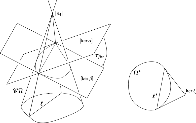
Figure 2: The cone $\mathscr{C}\Omega\subset\operatorname{\mathbb{R}\textrm{P}}^{3}$ with two hyperplanes intersecting it. The line $\ell$ is shown in $\mathbb{P}(\mathbb{R}^{4}/[e_{4}])$, and the dual data in $\Omega^{*}\subset\mathbb{P}(\operatorname{TAff}^{*}(3,\mathbb{R}))$.

Consider $\mathscr{C}\Omega=[Q]^{-1}(\Omega)$, which is an open cone in $\operatorname{\mathbb{R}\textrm{P}}^{3}\setminus\{[e_{4}]\}$. Topologically, the closure of this cone in $\operatorname{\mathbb{R}\textrm{P}}^{3}$ is the one point compactification of the product $\overline{\Omega}\times\mathbb{R}$, the exceptional point $[e_{4}]$ being the compactifying point. See Figure 2.

Since $\Omega\subset\mathbb{P}(\mathbb{R}^{4}/[e_{4}])$, $\Omega$ is actually equal to the set of lines which pass through $[e_{4}]$ and which intersect the cone $\mathscr{C}\Omega$. Let us call such lines the vertical lines in $\mathscr{C}\Omega$.

Choosing an orientation on a hyperplane $[\ker\alpha]$ where $\alpha\in(\operatorname{\mathbb{A}}^{3})^{*}$ amounts to choosing a lift of $[\alpha]$ which evaluates either positively or negatively on $e_{4}\in[e_{4}]$.

We consistently oriented $[\alpha]\in(\operatorname{\mathbb{A}}^{3})^{*}$ by insisting that $\alpha(e_{4})=+1$. Call these the (positively) oriented hyperplanes. Observe that the group of translations $\operatorname{TAff}^{*}(3,\mathbb{R})$ acts simply transitively on the positively oriented hyperplanes. The vertical lines are then oriented to point into the positive half-space of every positively oriented hyperplane.

Remark 3.5.

Choose an affine chart for $\operatorname{\mathbb{R}\textrm{P}}^{3}$ containing $\mathscr{C}\Omega$; $[e_{4}]$ is at infinity in such a chart. The cone $\mathscr{C}\Omega$ is a cylinder: $\Omega\times\mathbb{R}$ which is more evident in this chart. An orientation on this chart and on the $\mathbb{R}$-factor co-orients the hyperplanes which intersect $\mathscr{C}\Omega$. This cylinder is the generalization of Danciger’s ‘half-pipe’ model for co-Minkowski space [Dan13] (it is exactly this when $\Omega$ has boundary an ellipse). Ungemach calls this space $\mathbf{HP}(\Omega)$ [Ung19].

3.2 The minimal domain of a convex cocompact coaffine representation

This subsection is devoted to describing the geometry of the action of $\eta$ on $\operatorname{\mathbb{R}\textrm{P}}^{3}\setminus\{[e_{4}]\}$, which (from our perspective) is governed by its minimal convex domain of discontinuity.

Lemma 3.6.

For any $\varphi\in Z^{1}(\pi_{1}S,(\mathbb{R}^{3})^{*}_{\rho})$, the representation $\eta$ defined in (6) is projective Anosov and the limit curve $\operatorname{im}\xi$ is contained in $\partial\mathscr{C}\Omega\setminus\{[e_{4}]\}$.

Proof.

Consider the path of representations $\eta_{t\varphi}$ for $t\in[0,1]$. When $t=0$, $\eta_{0}$ is reducible; its Anosov limit curve is contained in the hyperplane $[\ker(e^{4})]\subset\operatorname{\mathbb{R}\textrm{P}}^{3}$ and is the boundary of the domain $\Omega$ inside of this embedded $\operatorname{\mathbb{R}\textrm{P}}^{2}$. Therefore the Lemma holds in this case.

Since the property of being projective-Anosov is open, there exists some $\epsilon>0$ so that the representation $\eta_{t\varphi}$ is projective-Anosov for all $t<\epsilon$. Since the limit map $\xi$ varies continuously in the representation, for sufficiently small $\epsilon$, $\operatorname{im}\xi$ is contained in $\partial\mathscr{C}\Omega\setminus\{[e_{4}]\}$.

Observe that the conjugate of $\eta_{t\varphi}$ by the element $\textrm{diag}(s^{-1/2},s^{-1/2},s^{-1/2},s^{3/2})\in\operatorname{SL}(4,\mathbb{R})$ is equal to $\eta_{(st)\varphi}$. Therefore the Lemma holds for arbitrary $\varphi\in Z^{1}(\pi_{1}S,(\mathbb{R}^{3})^{*}_{\rho})$ ∎

There is a minimal convex domain of discontinuity for the action of $\eta$ on $\operatorname{\mathbb{R}\textrm{P}}^{3}$.

$$\Xi=\operatorname{hull}(\operatorname{im}(\xi))\setminus\operatorname{im}(\xi).$$

Then $\Xi$ can also be realized as the intersection of all convex domains of discontinuity for the action of $\eta$ on $\operatorname{\mathbb{R}\textrm{P}}^{d}$.

Lemma 3.7.

The action of $\eta(\pi_{1}S)$ on $\Xi$ is cocompact with quotient homeomorphic to $S\times[0,1]$.

Proof.

It follows from Lemma 3.6 that $[e_{4}]$ is not contained in $\Xi$. Therefore there exist a pair of hyperplanes $H_{1}$ and $H_{2}$ bounding $\Xi$ from $[e_{4}]$. The projection $[Q]$ is $(\eta,\rho)$-equivariant, so the action of $\eta$ on $\Xi$ is proper.

Since $\Xi$ is convex, the pre-image of a point $p\in\Omega$ is a closed interval. Since $\eta$ preserves the orientations on the vertical lines of $\mathscr{C}\Omega$, this proves that

$$\Xi/\eta(\pi_{1}S)\cong\left(\Omega/\rho(\pi_{1}S)\right)\times[0,1].$$

The Lemma is complete. ∎

This is the converse of Lemma 3.1; convex cocompact coaffine representations and coaffine representations with Hitchin linear part are the same objects.

Remark 3.8.

Coaffine representations with Hitchin linear part are also strongly convex cocompact in the sense of [DGK23, Definition 1.1]. One should generally be concerned about the notions of ‘naive’ and ‘strong’ projective cocompactness, as discussed in [DGK23]. Since surface groups are non-elementary Gromov hyperbolic groups, the two notions coincide. See Theorem 1.15 of that paper.

Henceforth we fix $\eta$ and study the structure of $\Xi$. The following definition describes the sort of object that may be found naturally bounding $\Xi$.

Definition 3.9.

A bent domain is a triple $(D,\lambda,h)$ of a domain $D\subset\operatorname{\mathbb{R}\textrm{P}}^{2}$ with strictly convex boundary, a geodesic lamination (see §2.3) $\lambda$ on $D$, and a continuous map $h:D\rightarrow\operatorname{\mathbb{R}\textrm{P}}^{3}$ which satisfies

• For every leaf $\ell\subset\lambda$, $h|_{\ell}$ is a projective isomorphism to its image,

• For every connected component $P\subset D\setminus\lambda$, the map $h|_{P}$ is a projective isomorphism to its image,

• The map $h$ has a continuous extension to $\partial\lambda\subset\partial D$.

Remark 3.10.

The image of a bent domain does not have any obvious (intrinsic) global projective structure. In future work we will upgrade this definition to a more delicate notion generalizing pleated surfaces. For now, this definition suffices.

We will encounter maps which are simultaneously bent domains and sections of the cone $\mathscr{C}\Omega\rightarrow\Omega$. In particular, we wish to characterize when such maps have convex graphs in $\mathscr{C}\Omega$.

Because the vertical lines in $\mathscr{C}\Omega$ are oriented, it is coherent to discuss the positive and negative sides of a continuous section

$$q:\Omega\rightarrow\mathscr{C}\Omega.$$

Such a section divides $\mathscr{C}\Omega$ into two connected components, and any vertical line $L$ is oriented into the positive half of $\mathscr{C}\Omega\setminus\operatorname{im}q$.

This gives a concise definition of convexity in the cone $\mathscr{C}\Omega$ that matches the intuitive notion one might expect.

Definition 3.11.

A continuous section $q:\Omega\rightarrow\mathscr{C}\Omega$ is convex up (resp. down) if for all $x,y\in\Omega$, the segment $[q(x),q(y)]$ is contained in the closure of the positive (resp. negative) side of $\mathscr{C}\Omega\setminus\operatorname{im}q$.

Suppose that $q:\Omega\rightarrow\mathscr{C}\Omega$ is both a bent domain $(\Omega,\lambda,q)$ and a section (so that $[e_{4}]\notin\overline{\operatorname{im}q}$). For each connected component $P\subset\Omega\setminus\lambda$ let $\alpha(P)=\alpha(q,P)$ be the unique oriented hyperplane containing $q(P)$.

Then the following characterization of convexity holds

Lemma 3.12.

Let $q:\Omega\rightarrow\mathscr{C}\Omega$ be a bent domain and a section. The graph $\operatorname{im}q\subset\mathscr{C}\Omega$ is convex up if and only if for all $X,Y$ connected components of $\Omega\setminus\lambda$,

$$\alpha(Y)(q(X))\geq 0$$

where the inequality is read to mean that $q(X)$ is on the positive side of $\alpha(Y)$. A symmetric result holds for ‘convex down’.

Proof.

This amounts to a fact about functions from $\Omega^{\prime}\subset\mathbb{R}^{d}\rightarrow\mathbb{R}$ where $\Omega^{\prime}$ is strictly convex: such a function is convex if and only if its graph is contained in the boundary of its own convex hull. The condition is then the requirement that $\alpha(Y)$ be a supporting hyperplane to the convex hull of $\operatorname{im}q$. ∎

We can relate this condition for convexity to the geometry of $\Omega$. Given a geodesic lamination

$$\widetilde{\lambda}\subset\Omega,$$

the boundary pairs defining its leaves in the space of geodesics identify a geodesic lamination

$$\widetilde{\lambda}^{*}\subset\Omega^{*}.$$

More explicitly, the composition of the limit curves $\left(\xi^{*}\circ\xi^{-1}\right)$ defines a bijection between the set of geodesics in $\Omega$ and the set of geodesics in $\Omega^{*}$: a geodesic $\ell\subset\Omega$ with endpoints $\ell_{\pm}$ is mapped to the leaf $\ell^{*}\subset\Omega^{*}$ with endpoints $\ell^{*}_{\pm}$ which are the unique supporting hyperplanes to $\ell_{\pm}$. The image of a geodesic lamination under this map is a geodesic lamination.

Definition 3.13.

Let $\ell_{1}$ and $\ell_{2}$ be a pair of non-intersecting geodesics in a strictly convex and $C^{1}$ domain $\Omega\subset\operatorname{\mathbb{R}\textrm{P}}^{2}$, and $\ell^{*}_{1},\ell^{*}_{2}$ the dual geodesics in $\Omega^{*}$. Define the closed set

$$R(\ell_{1},\ell_{2})=\{[v]\in(\operatorname{\mathbb{R}\textrm{P}}^{2})\mid[\ker v]\cap\Omega^{*}~{}\textrm{between}~{}\ell^{*}_{1}~{}\textrm{and}~{}\ell^{*}_{2}.\}$$

Similarly define $R(\ell^{*}_{1},\ell^{*}_{2})$ symmetrically as a subset of $(\operatorname{\mathbb{R}\textrm{P}}^{2})^{*}$.

Let $[v_{1}]$ be the intersection of the two tangent lines to $\Omega$ at the endpoints of $\ell_{1}$ so that $\ell^{*}_{1}\subset[\ker v_{1}]\subset(\operatorname{\mathbb{R}\textrm{P}}^{2})^{*}$. Define $[v_{2}]$ similarly.

Lemma 3.14.

Suppose $\ell_{1}$ and $\ell_{2}$ do not share an endpoint. The subset $R(\ell_{1},\ell_{2})$ is equal to the closure of th connected component of

$$\operatorname{\mathbb{R}\textrm{P}}^{2}\setminus\left([\ker(\ell^{*}_{1})_{+}]\cup[\ker(\ell^{*}_{1})_{-}]\cup[\ker(\ell^{*}_{2})_{+}]\cup[\ker(\ell^{*}_{2})_{-}]\right)$$

which is characterized by being a $4$-gon, not containing $\Omega$, and having $[v_{1}]$ and $[v_{2}]$ in its closure (Figure 3).

When $\ell_{1}$ and $\ell_{2}$ share an endpoint, then $R(\ell_{1},\ell_{2})$ is the projective segment $[[v_{1}],[v_{2}]]\subset\operatorname{\mathbb{R}\textrm{P}}^{2}\setminus\overline{\Omega}$.

Proof.

The proof follows from the definitions and some projective geometry. See Figure 3. ∎

For $P\subset\Omega\setminus\lambda$, let $\mathscr{E}P\subset\operatorname{TAff}^{*}(3,\mathbb{R})$ be the set of translations $\tau$ so that $\tau.\alpha(P)$ evaluates positively on $P$. The set $\mathscr{E}P$ is a proper convex positive cone. Let $P_{1}$ and $P_{2}$ be a pair of distinct connected components in $\Omega\setminus\widetilde{\lambda}$, and let $\ell_{1}$ and $\ell_{2}$ be the extremal elements in the ordered set of leaves of $\widetilde{\lambda}$ between $P_{1}$ from $P_{2}$.

The following corollary is a restatement of Lemma 3.12:

Corollary 3.15.

The graph $\operatorname{im}q\subset\mathscr{C}\Omega$ is convex if and only if for all pairs of distinct connected components $P_{1},P_{2}$ in $\Omega\setminus\widetilde{\lambda}$, the difference

$$\alpha(P_{2})-\alpha(P_{1})\in\mathscr{E}P_{2}\cap(-\mathscr{E}P_{1}).$$

Also, the projectivization of $\mathscr{E}P_{2}\cap(-\mathscr{E}P_{1})$ is equal to $R(\ell^{*}_{1},\ell^{*}_{2}).$

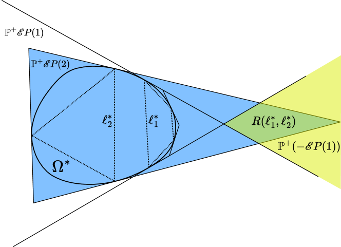
Figure 3: The relationship between $\mathscr{E}P(1)$, $\mathscr{E}P(2)$, and $R(\ell^{*}_{1},\ell^{*}_{2})$ in the positive projectivization of $\operatorname{TAff}^{*}(3,\mathbb{R})$.

Proof.

Figure 3 shows an affine chart for the positive projectivization of $\operatorname{TAff}^{*}(3,\mathbb{R})$, with the convex domain $\Omega^{*}$. The shaded region $\mathscr{E}P(1)$ is the dual domain of the stratum $P(1)$. It is necessary to work in the positive projectivization to preserve the meaning of signs, which give the notion of convexity. It is an exercise following from the definitions to show that the intersection of the two cones is $R(\ell^{*}_{1},\ell^{*}_{2})$ as claimed. ∎

The following lemma, also found in [Ung19], relates this conversation to coaffine convex cocompact representations. We supply a proof for completeness.

Lemma 3.16.

When $\varphi\notin B^{1}(\pi_{1}S,(\mathbb{R}^{3})^{*}_{\rho})$, the boundary $\partial\Xi\setminus\operatorname{im}(\xi)$ is a union of two disjoint (open) disks: $\partial\Xi\setminus\operatorname{im}(\xi^{1})=\partial\Xi^{+}\sqcup\partial\Xi^{-}.$ There exist natural maps

$$q^{\pm}:\Omega\rightarrow\partial\Xi^{\pm}$$

and laminations $\widetilde{\lambda}^{\pm}$ so that the $(\Omega,\widetilde{\lambda}^{\pm},q^{\pm})$ are bent domains. Furthermore, the maps $q^{\pm}$ are convex $(\rho,\eta)$-equivariant sections; i.e. for all $\gamma\in\pi_{1}S$, for all $x\in\Omega$

$$q^{\pm}\circ\rho(\gamma)(x)=\eta(\gamma)\circ q^{\pm}(x).$$

Proof.

The condition that $\varphi$ is not a coboundary is equivalent to requiring that $\eta$ preserves no hyperplane in $\operatorname{\mathbb{R}\textrm{P}}^{3}$ (Lemma 3.3). Therefore the limit curve $\operatorname{im}(\xi)$ is contained in no hyperplane, its convex hull $\overline{\Xi}$ is topologically a $3$-disk, and its boundary is topologically a $2$-sphere. The sets $\partial\Xi^{\pm}$ are then the complements in this $2$-sphere of the topological circle $\operatorname{im}(\xi)$.

The set $\Xi$ is a convex body properly contained in an affine chart, and so its boundary is stratified into a poset of faces (see [Roc70] for general background on convex geometry). Because $\Xi\subset\operatorname{\mathbb{R}\textrm{P}}^{3}$, the faces of $\Xi$ are of dimension $0$, $1$, or $2$. It is a fact (which is not difficult to prove) that every face $K$ of a proper convex set $X=\operatorname{hull}Y$ is the convex hull of some $Y^{\prime}\subset Y$. Applying this to the present situation, we conclude that every $0$-face of $\Xi$ must be in $\operatorname{im}(\xi)$. In particular, $\partial\Xi^{\pm}$ is a union of (open) $1$- and $2$-faces. Define $\widetilde{\lambda}^{\pm}$ to be the set of $1$-faces in $\partial\Xi^{\pm}$. The definition of a face of a convex body, together with the previous observation regarding $0$-faces is sufficient to conclude that $\widetilde{\lambda}^{\pm}$ are laminations on the disks $\partial\Xi^{\pm}$.

Recall from Equation (5) the natural projection $Q:\mathbb{R}^{4}\rightarrow\mathbb{R}^{4}/[e_{4}]$, and the induced projection

$$[Q]:\operatorname{\mathbb{R}\textrm{P}}^{3}\setminus\{[e_{4}]\}\rightarrow\mathbb{P}(\mathbb{R}^{4}/[e_{4}])\cong\operatorname{\mathbb{R}\textrm{P}}^{2}.$$

It is an exercise in projective geometry to see that the lines through $[e_{4}]$ contained in $\mathscr{C}\Omega$ intersect $\Xi$ in a proper segment. Define $q^{\pm}$ to be the inverse of the restriction of $[Q]$ to $\partial\Xi^{\pm}$. We may already conclude that $q^{\pm}$ are bijections. The fact that they are homeomorphisms to their images follows from the fact that their inverses are restrictions of the continuous map $[Q]$ to the graph of a convex section of $\mathscr{C}\Omega$.

To check that $[Q](\lambda^{\pm})$ are laminations on $\Omega$, one need only note that $[Q]$ is a projective map on each stratum, and that the set of leaves is closed. The closedness of the set of leaves follows from the fact that a Hausdorff limit of closed $n$-dimensional faces of a convex set is a closed face whose dimension is at most $n$.

The fact that $q^{\pm}$ is convex (up or down) in the sense of Definition 3.11 follows from Lemma 3.12 and the convexity of $\Xi$.

This completes the Lemma. ∎

The difference between the ‘positive’ and ‘negative’ data suggested by the ‘$\pm$’ decorations of the objects defined above is cosmetic, depending only on an orientation of the $\mathbb{R}$-factor of $\mathscr{C}\Omega$. There is no reason to favor either one over the other.

As it is a vector space, $(-I)$ acts on $Z^{1}(\pi_{1}S,(\mathbb{R}^{3})^{*}_{\rho})$ as an involution (which descends to $H^{1}(\pi,(\mathbb{R}^{3})^{*}_{\rho})$). This induces a nontrivial symmetry of the geometric data which we have been exploring. In particular, it exchanges $\partial\Xi^{+}$ and $\partial\Xi^{-}$. Explicitly, this is effected by conjugation by the $\operatorname{GL}(4,\mathbb{R})$ element $\textrm{diag}(1,1,1,-1)$.

3.3 Macroscopic bending data

In this subsection, we extract the ‘macroscopic bending data’ from $\partial\Xi$. We work with the same set-up and notation from the previous subsection: assume that $\varphi\in Z^{1}(\pi_{1}S,(\mathbb{R}^{3})^{*}_{\rho})$ is not a coboundary, and construct the corresponding coaffine convex cocompact representation $\eta=\eta_{\varphi}$. Let $\widetilde{\lambda}=[Q](\widetilde{\lambda}^{+})\subset\Omega$.

Remark 3.17.

Suppose that $\widetilde{\lambda}$ has an isolated leaf $\ell$ with a pair of adjacent $2$-faces supported by hyperplanes $\alpha$ and $\beta$ (such a leaf does not always exist). The discussion in §3 shows that the difference $[\beta-\alpha]\in[\ker\ell]\subset\mathbb{P}\operatorname{TAff}^{*}(3,\mathbb{R})$. See Figure 2 for the geometric meaning of $[\ker\ell]$. This section generalizes this localization property of the bending data to the case of non-isolated leaves of the bending lamination on $\partial\Xi$.

From the discussion in the previous subsection, it is evident that for any $x\in\Omega\setminus\widetilde{\lambda}$, there exists a unique supporting hyperplane $[\ker\alpha(x)]$ to $\Xi$ at $q^{+}(x)\in\partial\Xi$, where $\alpha(x)\in(\operatorname{\mathbb{A}}^{3})^{*}$. Thus the following is well-defined:

Definition 3.18.

Let $[\eta]$ be the $\operatorname{TAff}^{*}(3,\mathbb{R})$ conjugacy class of a coaffine representation with Hitchin linear part $L(\eta)=\rho$. The bending cocycle $\psi=\psi([\eta])$ is defined as follows.

To an arc $k:[0,1]\rightarrow\Omega$ with endpoints not in $\widetilde{\lambda}$, let

$$\psi(k)=\alpha(k(1))-\alpha(k(0))\in\operatorname{TAff}^{*}(3,\mathbb{R}).$$

Some elementary properties of $\psi$ are evident from the definitions.

Lemma 3.19.

The map $\psi$ satisfies the following properties

• Equivariance: $\psi(\gamma.k)=\rho(\gamma).\psi(k)$ for all arcs transverse to $\widetilde{\lambda}$ and $\gamma\in\pi_{1}S$.

• Transverse isotopy invariance: $\psi$ only depends on the two-strata containing $\partial k$.

• Support: $\psi(k)=0$ if and only if $\partial k$ is contained in some component of $\Omega\setminus\widetilde{\lambda}$.

• Flip equivariance: For an oriented arc $k$, if $\bar{k}$ denotes $k$ with the opposite orientation, then $\psi(\bar{k})=-\psi(k)$.

• Additivity: if $k=k_{1}\cdot k_{2}$, then $\psi(k)=\psi(k_{1})+\psi(k_{2})$.

As one might hope, $\psi$ is related to the cocycle $\varphi$ (defining $\eta$) in the following precise sense.

Lemma 3.20.

Let $p\in\Omega\setminus\widetilde{\lambda}$, and for all $\gamma\in\pi_{1}S$ let $\widetilde{\gamma}$ be the unique lift of $\gamma$ to $\Omega$ based at $p$ (considered up to isotopy relative to its boundary). Then

$$[\gamma\mapsto\psi(\widetilde{\gamma}^{-1})]=\varphi\in H^{1}(\pi_{1}S,\operatorname{TAff}^{*}(3,\mathbb{R})_{\rho}).$$

Proof.

Let $P\subset\Omega\setminus\widetilde{\lambda}$ be the connected component containing $p$. Conjugacy affects the addition of a coboundary, so it is sufficient to prove the lemma when $\alpha(P)=[\ker e^{4}]$. In this case, a matrix computation completes the proof:

$$\eta(\gamma).e^{4}=e^{4}+\varphi(\gamma^{-1}).$$

∎

Choose any auxiliary Riemannian metric $d_{\mathbb{P}}$ on $\operatorname{\mathbb{R}\textrm{P}}^{2}$. Having now defined $\psi$, revisiting Corollary 3.15 implies the following useful property.

Corollary 3.21.

There is an $a\in(0,1)$ such that when $k$ is an arc transverse to $\widetilde{\lambda}$ and $\ell_{x}$ is a leaf of $\widetilde{\lambda}$ intersecting $k$ non-trivially, then $d_{\mathbb{P}}(\psi(k),\ell_{x})=O(\operatorname{diam}k^{a})$.

Additionally, there exists a proper positive convex cone $\mathscr{E}\subset\operatorname{TAff}^{*}(3,\mathbb{R})$ so that for all subarcs $k^{\prime}$ of $k$, $\psi(k^{\prime})\in\mathscr{E}$.

Proof.

Let $\ell_{1}$ and $\ell_{2}$ be the first and last leaf of $\widetilde{\lambda}$ which $k$ intersects non-trivially. First observe (from the definition) that $\ell_{x}\in R(\ell_{1}^{*},\ell_{2}^{*})$. So we must only understand how the parallelogram $R(\ell^{*}_{1},\ell^{*}_{2})$ varies in the arc $k$.

Recall that $\partial\pi_{1}S$ has a visual metric after choosing a hyperbolic structure $S\cong X$, which is unique up to bi-Hölder equivalence. Then in the model geometry of $T^{1}X$, the map from (oriented) points in a geodesic lamination to their endpoints in $\partial\pi_{1}S$ is Lipschitz. The limit curve $\xi:\partial\pi_{1}S\rightarrow\operatorname{\mathbb{R}\textrm{P}}^{2}$ is $a$-Hölder, for some $a\in(0,1)$. So $R(\ell^{*}_{1},\ell^{*}_{2})$ is a convex hull of four points in $\operatorname{\mathbb{R}\textrm{P}}^{2}$, the distance between any two of which varies Hölder in $\operatorname{diam}k$. The result then follows as the diameter of $R(\ell^{*}_{1},\ell^{*}_{2})$ varies Hölder in $\operatorname{diam}k$.

The necessary cone $\mathscr{E}$ is one component of the cone over $R(\ell_{1}^{*},\ell_{2}^{*})\subset\mathbb{P}\operatorname{TAff}^{*}(3,\mathbb{R})$. Corollary 3.15 and a short geometric argument complete the proof. ∎

Remark 3.22.

We may treat $\psi$ as in Definition 3.18 as an element of $Z^{1}(S,F^{\rho})$. Let $k$ be an arc transverse to $\lambda$, and define

$$\psi(k)=\overline{k}_{*}\alpha(k(1))-\alpha(k(0))$$

where $\overline{k}_{*}$ is $\nabla^{\rho}$-parallel transport along $k$.

4 Equivariant transverse measures

When the linear part $\rho:\pi_{1}S\to\operatorname{SL}(3,\mathbb{R})$ of $\eta:\pi_{1}S\to\operatorname{Aff}^{*}(3,\mathbb{R})$ is Fuchsian, there is a global $\nabla^{\rho}$-flat section of $E_{2}^{\rho}\to T^{1}S$. In this classical setting, the bending data on a component of the convex core boundary takes the form of a transverse measure whose support is the bending lamination. For a fixed hyperbolic metric, measured laminations embed into flow invariant measures on the unit tangent bundle.

In general, there is no global flat section of $E^{\rho}_{2}\to T^{1}S$. Instead, choose (for the remainder of this section) two auxiliary structures: a smooth norm $\|\cdot\|$ on $E^{\rho}$ and a hyperbolic metric $X$ on $S$ with geodesic flow $g_{t}:T^{1}X\to T^{1}X$. Let $\pi:T^{1}X\to X$ denote the tangent projection and $p\mapsto\overline{p}$ the antipodal involution of $T^{1}X$, which satisfies $g_{t}\overline{p}=\overline{g_{-t}p}$.

Consider the smooth function $G:T^{1}X\times\mathbb{R}\to\mathbb{R}_{>0}$ defined by

$$G(p,t)=\frac{\|\left(g_{[0,t]}\right)_{*}v\|_{g_{t}p}}{\|v\|_{p}},~{}v\in E_{2}^{\rho}|_{p},$$ (7)

which measures the distortion of $\|\cdot\|$ along $g_{t}$-orbits of the $\nabla^{\rho}$-parallel transport. A measure on the unit tangent bundle of $X$ is $(g,G)$-equivariant if it scales by $G$ under the flow $g$ (see Equation (8)). The set of $(g,G)$-equivariant measures with support tangent to a lamination (Definition 4.1) parameterizes conjugacy classes of coaffine representations with linear part $\rho$ (Theorem 5.1).

Note that the function $G=G(\rho)$ varies continuously in the connection $\nabla^{\rho}$.

In §4.1, we characterize which geodesic laminations support equivariant measures for a given $\rho$ in terms of the exponential growth of $G$ along its leaves (Corollary 4.7). Theorem 4.10 then demonstrates that every non-orientable geodesic lamination is the support of an equivariant measure.

In §4.2, we disintegrate a flow equivariant measure on a transversal to obtain an equivariant transverse measure (Definition 4.13), and show that this assignment is a homeomorphism (Proposition 4.17). Ultimately, we are interested in these transverse measures, as the interesting part of a flow equivariant measure lives in the transverse direction to the flow.

4.1 Building flow equivariant measures

Let $\mathcal{M}(T^{1}X)$ be the space of finite Borel measures on $T^{1}X$ with its weak-$*$ topology. We say that $\nu\in\mathcal{M}(T^{1}X)$ is $(g,G)$-equivariant if

$$d\left(g_{t}\right)_{*}\nu=G(\cdot,-t)d\nu$$ (8)

holds for all $t\in\mathbb{R}$. In other words, $\nu$ and $\left(g_{t}\right)_{*}\nu$ are mutually absolutely continuous with Radon-Nykodym derivative given by $G(\cdot,-t)$. Thus, when $\rho$ is Fuchsian, there is a bilinear form on $E^{\rho}$ and hyperbolic metric making $G\equiv 1$.

Definition 4.1.

Denote by $\mathcal{ML}(T^{1}X)^{G}\subset\mathcal{M}(T^{1}X)$ the set of $(g,G)$-equivariant finite Borel measures $\nu$ that are invariant under the antipodal involution and that have support $\widehat{\lambda}$, where $\lambda\subset X$ is a geodesic lamination and $\widehat{\lambda}=T^{1}\lambda$ is its set of tangents.

Note that $\mathcal{ML}(T^{1}X)^{G}$ is equipped with the topology of weak-$*$ convergence as a subspace of $\mathcal{M}(T^{1}X)$.

The following basic properties of $G$ are easily verified.

Lemma 4.2.

For all $p\in T^{1}S$ and $s,t\in\mathbb{R}$, we have

$$G(p,s+t)=G(p,s)G(g_{s}p,t),$$

and

$$G(\overline{p},-t)=G(p,t).$$

Furthermore, for all $T$, we have

$$\int_{-T}^{T}G(p,t)~{}dt=\int_{-T}^{T}G(\overline{p},t)~{}dt.$$

The key to building $(g,G)$-equivariant measured laminations is understanding the accumulation of holonomy along $g_{t}$-orbits. Define

$$\Lambda^{+}(p)=\limsup_{t\to\infty}\frac{1}{t}\log G(p,t),$$

and

$$\Lambda^{-}(p)=\liminf_{t\to\infty}\frac{1}{t}\log G(p,t),$$

which are Borel measurable functions on $T^{1}X$. Note that the signs of $\Lambda^{\pm}$ depend neither on our choice of negatively curved metric (hence parameterization of the geodesic flow) nor on our choice of norm $\|\cdot\|$. Continuity of $G$ ensures that $-\infty<\Lambda^{\pm}<+\infty$.

Remark 4.3.

The functions $\Lambda^{\pm}$ measure the exponential growth rate of the middle singular value in matrix products corresponding to an infinite word $\gamma_{1}\cdot\gamma_{2}\cdot...$ encoding the geodesic trajectory $\{g_{t}p:t\geq 0\}$ under $\rho$. We note that if $p$ is generic for a $g_{t}$-invariant ergodic probability measure supported on $\widehat{\lambda}$, then continuity of $G$ ensures that $\Lambda^{+}(p)=\Lambda^{-}(p)$, and this quantity can be computed by integrating the derivative of $G$; see the proof of Theorem 4.10. One can view this in the framework of Lyapunov exponents and the Ergodic Theorem.

The following lemma supplies a necessary condition for a geodesic lamination to support of an equivariant measure.

Lemma 4.4.

For a given $\nu\in\mathcal{ML}(T^{1}X)^{G}$, $\nu$-a.e. point $p$ has $\Lambda^{+}(p)\leq 0$ and $\Lambda^{+}(\overline{p})\leq 0$.

Proof.

By equivariance, for all continuous functions $f:T^{1}X\to\mathbb{R}$, we have

$$\int f~{}d\nu=\int f\circ g_{T}\cdot G(\cdot,T)~{}d\nu$$

for all $T\in\mathbb{R}$. In particular,

$$\nu(T^{1}X)=\int G(\cdot,T)~{}d\nu$$ (9)

for all $T\in\mathbb{R}$. Consider the set

$$B_{T}^{\epsilon}=\{p:G(p,T)\geq e^{\epsilon|T|}\}.$$

Then (9) implies that

$$\nu(B_{T}^{\epsilon})\leq\frac{\nu(T^{1}X)}{e^{\epsilon|T|}},$$

and so

$$\sum_{n=1}^{\infty}\nu(B_{n}^{\epsilon})<\infty$$

for all $\epsilon>0$. By the Borel-Cantelli Lemma,

$$\nu(\limsup_{n\to\infty}B_{n}^{\epsilon})=0,$$

which in particular implies that $\Lambda^{+}(p)<\epsilon$ for all positive $\epsilon$ and $\nu$-a.e. $p$. Using the fact that $G(p,-T)=G(\overline{p},T)$, a symmetric argument proves also that $\Lambda^{+}(\overline{p})\leq 0$ for $\nu$-a.e. $p$. The intersection of two $\nu$-full measure sets has full measure, proving the lemma. ∎

Now we give sufficient conditions for a minimal geodesic lamination to be the support of an equivariant measure.

Proposition 4.5.

Let $\lambda\subset X$ be a minimal geodesic lamination and $p\in\widehat{\lambda}$.

If $\int_{-\infty}^{\infty}G(p,t)~{}dt<\infty$, then $\widehat{\lambda}$ is the support of a measure $\nu\in\mathcal{ML}(T^{1}X)^{G}$ whose mass is concentrated on exactly two $g_{t}$-orbits that are exchanged by $p\mapsto\overline{p}$.

If $\int_{0}^{\infty}G(p,t)~{}dt=\infty$ and $0\in[\Lambda^{-}(p),\Lambda^{+}(p)]$ then $\widehat{\lambda}$ is the support of a measure $\nu\in\mathcal{ML}(T^{1}X)^{G}$.

Before proving the proposition, we prove a technical fact.

Lemma 4.6.

Suppose $f:\mathbb{R}\to\mathbb{R}$ is continuous and positive, and assume that for every $s>0$, there exists $D(s)>0$ so that when $\absolutevalue{u-u^{\prime}}<s$, the inequality $D(s)<f(u)/f(u^{\prime})<1/D(s)$ holds.

Then if there is some $s_{0}$ and sequence $T_{i}\to\infty$ satisfying

$$\inf_{T_{i}}\frac{\int_{T_{i}-s_{0}}^{T_{i}}f(t)~{}dt}{\int_{0}^{T_{i}}f(t)~{}dt}>0,$$

it is true that $\liminf_{i\to\infty}\frac{1}{T_{i}}\log f(T_{i})>0$.

Proof.

Consider the discrete analogue: suppose that $a_{n}$ is a sequence of positive real numbers so that

$$\inf_{n}\frac{a_{n}}{\sum_{i=0}^{n}a_{i}}>0.$$

Then there is some $\epsilon$ so that $0<\epsilon<1$ so that for all $n>0$, $a_{n}>\varepsilon\sum_{i=0}^{n}a_{i}$. By an inductive argument using the binomial theorem, one may deduce that for every $n$,

$$a_{n}>\frac{\epsilon}{(1-\epsilon)^{n}}a_{0}.$$

In other words, $\liminf_{n\rightarrow\infty}\frac{1}{n}\log(a_{n})>0$.

To generalize to the continuous case, firstly assume without loss of generality that the sequence $T_{i}$ is increasing and that $\absolutevalue{T_{i+1}-T_{i}}>2s$. It is then possible to partition each subinterval $[T_{i},T_{i+1}]$ into subintervals $J_{j}$ of diameter in $[0,s]$ so that for every $i$ there is some $j_{i}$ with $[T_{i}-s,T_{i}]=J_{j_{i}}$, and so that $j_{i}/T_{i}>1/(2s)$.

Then consider the sequence $a_{j}=\int_{J_{j}}f~{}dt$ and the subsequence $a_{j_{i}}$, which satisfies the assumption of the discrete case. Therefore there is a positive $\varepsilon$ such that

$$\frac{1}{T_{i}}\log\int_{T_{i}-s}^{T_{i}}f~{}dt>\frac{1}{2s}\frac{1}{j_{i}}\log a_{j_{i}}>\varepsilon.$$

To pass from the statement about the integral over $[T_{i}-s,T_{i}]$ to the evaluation $f(T_{i})$ requires the assumption about the variation of $f$. By the intermediate value theorem, there exists some $t_{i}^{*}\in[T_{i}-s,T_{i}]$ so that $sf(t_{i}^{*})=\int_{T_{i}-s}^{T_{i}}f(t)~{}dt$. Then for $i$ large enough, $\frac{1}{T_{i}}\log f(T_{i})>\epsilon$ holds, proving the Lemma. ∎

Proof of the Proposition.

If $G(p,\cdot)$ is integrable then so is $G(\overline{p},\cdot)$ by Lemma 4.2. Then

$$\nu=\int_{-\infty}^{\infty}G(p,t)\delta_{g_{t}p}~{}dt+\int_{-\infty}^{\infty}G(\overline{p},t)\delta_{g_{t}\overline{p}}~{}dt$$

is a finite Borel measure on $T^{1}X$. The support of $\nu$ is $\widehat{\lambda}$, because $\{g_{t}p\}_{t>0}$ is dense in the connected component of $\widehat{\lambda}$ containing $p$ (see §2.3). The $(g,G)$-equivariance of $\nu$ follows essentially from the cocycle property satisfied by $G$. Namely, for any continuous function $f:T^{1}X\to\mathbb{R}$, we have

$$\int f~{}d(g_{t})_{*}\nu=\int_{-\infty}^{\infty}G(p,s)f(g_{t+s}p)~{}ds+\int_{-\infty}^{\infty}G(\overline{p},s)f(g_{t+s}\overline{p})~{}ds.$$

Changing variables $u=t+s$ and applying Lemma 4.2, the right hand side becomes

$$\int_{-\infty}^{\infty}G(p,u)G(g_{u}p,-t)f(g_{u}p)~{}du+\int_{-\infty}^{\infty}G(\overline{p},u)G(g_{u}\overline{p},-t)f(g_{u}\overline{p})~{}du=\int fG(\cdot,-t)~{}d\nu,$$

which proves equivariance.

For the other case, we give a variant of a standard argument of Krylov-Bogoliubov. Suppose now that $\int_{0}^{\infty}G(p,t)~{}dt=\infty$ and $0\in[\Lambda^{-}(p),\Lambda^{+}(p)]$. For $T>0$, define

$$\nu_{T}=\frac{1}{\int_{0}^{T}G(p,t)~{}dt}\int_{0}^{T}G(p,t)\delta_{g_{t}p}~{}dt.$$ (10)

Later, we will symmetrize with respect to the antipodal involution. Since $G(p,\cdot)$ is continuous, and $0\in[\Lambda^{-}(p),\Lambda^{+}(p)]$, there is a sequence $T_{i}$ tending to infinity with

$$\lim_{i\to\infty}\frac{1}{T_{i}}\log G(p,T_{i})=0.$$

The cocyle property of $G$ and uniform continuity implies that

$$\frac{G(\cdot,t)}{G(\cdot,t+u)}$$

is bounded uniformly (in terms of $s$) above and below for all $u\in[0,s]$. Then Lemma 4.6 implies then that for any $s\in\mathbb{R}$

$$\frac{\int_{T_{i}-s}^{T_{i}}G(p,t)~{}dt}{\int_{0}^{T_{i}}G(p,t)~{}dt}\to 0,~{}i\to\infty.$$ (11)

We claim that any weak-$*$ accumulation of $\{\nu_{T_{i}}\}$ is $(g,G)$-equivariant. Suppose $\nu$ is such an accumulation point (which exists by compactness of $\mathcal{M}(P^{1}X)$), and let $f:T^{1}X\to\mathbb{R}$ be continuous and $\epsilon>0$. Then

$$\left|\int f\circ g_{s}~{}d\nu-\int fG(\cdot,-s)d\nu\right|\leq \left|\int f\circ g_{s}~{}d\nu-\int f\circ g_{s}~{}d\nu_{T_{i}}\right|+$$

$$\left|\int f\circ g_{s}~{}d\nu_{T_{i}}-\int fG(\cdot,-s)~{}d\nu_{T_{i}}\right|+\left|\int fG(\cdot,-s)~{}d\nu_{T_{i}}-\int fG(\cdot,-s)~{}d\nu\right|$$

The first and last terms are smaller than $\epsilon$ for $i$ large engouh by weak-$*$ convergence of $\nu_{T_{i}}\to\nu$ (after passing to a subsequence) and because $f\circ g_{s}$ and $fG(\cdot,-s)$ are both continuous. Consider the middle term, which is equal to

$$\frac{1}{\int_{0}^{T_{i}}G(p,t)~{}dt}\left|\int_{0}^{T_{i}}G(p,t)f(g_{t+s}p)~{}dt-\int_{0}^{T_{i}}G(p,t)G(g_{t}p,-s)f(g_{t}p)~{}dt\right|$$

After changing variables and applying the cocycle property of $G$, this becomes

$$\frac{1}{\int_{0}^{T_{i}}G(p,t)~{}dt}\left|\int_{-s}^{0}G(p,t)G(g_{t}p,-s)f(g_{t}p)~{}dt-\int_{T_{i}-s}^{T_{i}}G(p,t)G(g_{t}p,-s)f(g_{t}p)~{}dt\right|,$$

which is bounded by the sum of the ratios. Then the numerator in

$$\frac{\int_{-s}^{0}|G(p,t)G(g_{t}p,-s)f(g_{t}p)|~{}dt}{\int_{0}^{T_{i}}G(p,t)~{}dt}$$

is bounded because of continuity and compactness, while the denominator goes to infinity. For the second term, we have

$$\frac{\int_{T_{i}-s}^{T_{i}}|G(p,t)G(g_{t}p,-s)f(g_{t}p)|~{}dt}{\int_{0}^{T_{i}}G(p,t)~{}dt}\leq\|G(\cdot,-s)\|_{\infty}\|f\|_{\infty}\frac{\int_{T_{i}-s}^{T_{i}}G(p,t)~{}dt}{\int_{0}^{T_{i}}G(p,t)~{}dt},$$

which tends to zero by (11); in particular, both terms are smaller than $\epsilon$ for $i$ large enough. Since $\epsilon>0$ was arbitrary, this proves that $\nu$ is equivariant.

Using the property $G(\overline{p},-t)=G(p,t)$, one can see that $\overline{\nu}$, i.e., the pushforward of $\nu$ via the antipodal involution, is $(g,G)$-equivariant as well. Thus $\nu+\overline{\nu}$ is symmetric, equivariant, and its support is $\widehat{\lambda}$. This completes the proof. ∎

Thus we obtain a characterization of which minimal laminations support equivariant measures on their orientation covers.

Corollary 4.7.

Let $\lambda\subset X$ be a minimal geodesic lamination. Then $\widehat{\lambda}$ is the support of some $\nu\in\mathcal{ML}(T^{1}X)^{G}$ if and only if there exists $p\in\widehat{\lambda}$ satisfying $\Lambda^{+}(p)\leq 0$ and $\Lambda^{+}(\overline{p})\leq 0$.

Proof.

Sufficiency is proved using Proposition 4.5: If there exists such a $p$, then either $\int_{-\infty}^{\infty}G(p,t)~{}dt<\infty$ or the same integral is divergent and any weak-$*$ accumulation point of $\nu_{T}$ defined as in (10) is $(g,G)$-equivariant. After symmetrizing with respect to $p\mapsto\overline{p}$, this produces a measure $\nu\in\mathcal{ML}(T^{1}X)^{G}$ with support equal to $\widehat{\lambda}$.

Necessity is the content of Lemma 4.4. ∎

Remark 4.8.

It is possible also to deduce from Hurewicz’s Ergodic Theorem [Aar97, Theorem 2.2.1] and the Ergodic Decomposition Theorem for finite quasi-invariant Borel measures with a given Radon-Nikodym derivative ([GS00] or [Aar97]) that every ergodic $(g,G)$-equivariant measure $\nu$ supported in $\widehat{\lambda}$ has a generic point. That is, there is a point $p$ such that both

$$\frac{\int_{0}^{T}G(p,t)\delta_{g_{t}p}~{}dt}{\int_{0}^{T}G(p,t)~{}dt}\to\nu\text{ and }\frac{\int_{0}^{T}G(p,-t)\delta_{g_{-t}p}~{}dt}{\int_{0}^{T}G(p,-t)~{}dt}\to\nu$$

weak-$*$ as $T\to\infty$. The argument can be found in a first course on ergodic theory, and relies on separability of space of continuous functions on a compact metric space. See, e.g., [EW11, Corollary 4.12]. That Hurewicz’s Ergodic theorem for $\mathbb{Z}$-actions can be extended to $\mathbb{R}$-actions can be deduced from the proof of [EW11, Corollary 8.15].

Here is another way to build an equivariant measure from a geodesic that spirals onto minimal laminations where $G$ decays exponentially in both directions along $\ell$. Such a measure will have all of its mass concentrated along a single $g_{t}$-orbit and its time reversal.

Lemma 4.9.

Suppose $\lambda$ and $\lambda^{\prime}$ are minimal geodesic laminations on $X$, and suppose $\ell$ is isolated leaf spiraling onto $\lambda$ and $\lambda^{\prime}$ in such a way that $\lambda\cup\ell\cup\lambda^{\prime}$ is a geodesic lamination. Let $p\in\widehat{\ell}$ such that $\{g_{t}p\}_{t\geq 0}$ is asymptotic to $\{g_{t}q\}_{t\geq 0}\subset\widehat{\lambda}$ and $\{g_{t}p\}_{t\leq 0}$ is asymptotic to $\{g_{t}q^{\prime}\}_{t\leq 0}\subset\widehat{\lambda}^{\prime}$.

If $\Lambda^{+}(q)<0$ and $\Lambda^{+}(\overline{q}^{\prime})<0$, then there is a $\nu\in\mathcal{ML}(T^{1}X)^{G}$ giving full measure to $\widehat{\ell}$ whose support is equal to $\widehat{\lambda}\cup\widehat{\ell}\cup\widehat{\lambda}^{\prime}$.

Proof.

Since $\log G(\cdot,T)$ is uniformly continuous (for any $T$) and the distance between $g_{t}p$ and $g_{t+s}q$ goes to zero in $t$ for some $s\in\mathbb{R}$, $\Lambda^{+}(p)=\Lambda^{+}(q)<0$. Similarly, $\Lambda^{+}(\overline{p})=\Lambda^{+}(\overline{q}^{\prime})<0$. Together, this implies that

$$\int_{-\infty}^{\infty}G(p,t)~{}dt<\infty,$$

so applying Proposition 4.5 gives the result. ∎

With help from the previous Lemma, we can now conclude one of the main results from this section. For context, there is a Thurston measure on $\mathcal{ML}(S)$ in the class of Lebesgue, and almost every measured lamination is minimal, maximal (hence non-orientable), and uniquely ergodic (see §2.3).

The following states, in particular, that every non-orientable minimal geodesic lamination is the support of an equivariant measure, independent of the linear part $\rho$.

Theorem 4.10.

Every non-orientable minimal geodesic lamination $\lambda$ has that $\widehat{\lambda}$ is the support of some $\nu\in\mathcal{ML}(T^{1}X)^{G}$.

Every uniquely ergodic orientable geodesic lamination $\lambda$ is contained in a geodesic lamination $\lambda^{\prime}$ satisfying that $\widehat{\lambda}^{\prime}$ is the support of some $\nu\in\mathcal{ML}(T^{1}X)^{G}$.

Proof of Theorem 4.10.

Suppose $\lambda\subset X$ is minimal, and consider a $\{g_{t}\}$-invariant ergodic probability measure $\mu$ with support contained in $\widehat{\lambda}$. The antipodal involution $p\mapsto\overline{p}\in T^{1}X$ induces simplicial involution of the space of $\{g_{t}\}$-invariant probability measures on $\widehat{\lambda}$; denote by $\overline{\mu}$ the pushforward of $\mu$ under the involution. Then $\overline{\mu}$ is ergodic and if $p$ is generic for $\mu$ then $\overline{p}$ is generic for $\overline{\mu}$. By generic, we mean that both

$$\frac{1}{T}\int_{0}^{T}\delta_{g_{t}p}~{}dt\text{ and }\frac{1}{T}\int_{0}^{T}\delta_{g_{-t}p}~{}dt$$

converge weak-$*$ to $\mu$ as $T\to\infty$. Moreover, $\mu$-a.e. $p$ is generic.

By the choice of a smooth norm $\|\cdot\|$ on $E^{\rho}$ and because the flow $g_{t}$ and flat connection $\nabla^{\rho}$ are all smooth, $G(p,t)$ is continuously differentiable in $t$. Denote by

$$G^{\prime}(p,t)=\left.\frac{d}{ds}\right|_{s=t}G(p,s).$$

Using the cocycle property of $G$, one verifies

$$G^{\prime}(p,t)=G(p,t)G^{\prime}(g_{t}p,0)~{}\text{ for all $t\in\mathbb{R}$}.$$

The Fundamental Theorem of Calculus provides

$$\frac{1}{T}\log G(p,T)=\frac{1}{T}\int_{0}^{T}G^{\prime}(g_{t}p,0)~{}dt.$$

Since $p$ is generic for $\mu$, we obtain

$$\Lambda(p):=\lim_{T\to\infty}\frac{1}{T}\log G(p,t)=\int G^{\prime}(\cdot,0)~{}d\mu,$$

so that $\Lambda^{+}(p)=\Lambda(p)=\Lambda^{-}(p)$ holds.

Genericity of $p$ for $\mu$ implies also that its backward $g_{t}$ orbit equidistributes to $\mu$, so additionally:

$$\lim_{T\to\infty}\frac{1}{T}\int_{0}^{T}G^{\prime}(g_{-t}p,0)~{}dt=\int G^{\prime}(\cdot,0)~{}d\mu=\Lambda(p).$$

On the other hand,

$$\frac{1}{T}\int_{0}^{T}G^{\prime}(g_{-t}p,0)~{}dt=\frac{1}{T}\int_{-T}^{0}G^{\prime}(g_{t}p,0)~{}dt=-\frac{1}{T}\log G(p,-T)=-\frac{1}{T}\log G(\overline{p},T),$$

where we used the property $G(p,t)=G(\overline{p},-t)$. Taking the limit as $T\to\infty$ yields

$$\int G^{\prime}(\cdot,0)~{}d\mu=\Lambda(p)=-\Lambda(\overline{p})=-\int G^{\prime}(\cdot,0)~{}d\overline{\mu}.$$

It follows that if $\mu=\overline{\mu}$, then $\Lambda(p)=0$ for every $\mu$-generic point $p$. Otherwise, $\Lambda(p)=-\Lambda(\overline{p})$ holds for all $\mu$-generic points $p$.

Case: $\lambda$ is non-orientable. That $\lambda$ is non-orientable implies that $\widehat{\lambda}$ is connected and $g_{t}$-minimal. If $\Lambda(p)=0=\Lambda(\overline{p})$ we can apply Proposition 4.5. Indeed, either $\int_{-\infty}^{\infty}G(p,t)~{}dt<\infty$ or otherwise one of

$$\int_{0}^{\infty}G(p,t)~{}dt\text{ and }\int_{-\infty}^{0}G(p,t)~{}dt=\int_{0}^{\infty}G(\overline{p},t)~{}dt$$

is infinite.

Otherwise, $\Lambda(p)\not=\Lambda(\overline{p})$ and so $\mu\not=\overline{\mu}$.

Claim 4.11.

There is some $p\in\widehat{\lambda}$ with $0\in[\Lambda^{-}(p),\Lambda^{+}(p)]$ and $0\in[\Lambda^{-}(\overline{p}),\Lambda^{+}(\overline{p})]$.

Proof of the claim.

Without loss of generality, we assume that $L=\Lambda(p)>0$, so that $-L=\Lambda(\overline{p})<0$. Since $\frac{1}{T}\log G(\cdot,T)$ is continuous for every $T$, the sets

$$U_{N}=\{p:\exists n\geq N\text{ s.t. }\frac{1}{n}\log G(p,n)\geq L/2\}\text{ and }V_{N}=\{p:\exists n\geq N\text{ s.t. }\frac{1}{n}\log G(p,n)\leq-L/2\}$$

are open. Moreover, $U_{N}$ and $V_{N}$ are dense for all $N$. Indeed, $U_{N}$ contains the $\mu$-generic points and $V_{N}$ contains the $\overline{\mu}$-generic points; genericity is an invariant of the $g_{t}$-orbit and $\widehat{\lambda}$ is minimal.

Since $\widehat{\lambda}$ is a Baire-space, the set

$$\left(\bigcap_{N}U_{N}\right)\bigcap\left(\bigcap_{N}V_{N}\right)$$

is dense $G_{\delta}$. This means that there is a point $p$ satisfying that $\frac{1}{n}\log G(p,n)$ is at least $L/2$ for infinitely many positive values of $n$ and at most $-L/2$ for infinitely many positive values of $n$.

Running the same argument in backwards time provides a dense $G_{\delta}$ set of points satisfying $0\in[\Lambda^{-}(\overline{p}),\Lambda^{+}(\overline{p})]$. The intersection of dense $G_{\delta}$ sets is dense $G_{\delta}$, which proves the claim. ∎

As we did earlier, we can now appeal to Proposition 4.5 to finish the proof in the case that $\lambda$ is non-orientable.

Case: $\lambda$ is orientable and uniquely ergodic. As before, if $\Lambda(p)=0=\Lambda(\overline{p})$ for all $\mu$-generic points $p$, then we just appeal to Proposition 4.5 to construct a measure $\nu\in\mathcal{ML}(T^{1}X)^{G}$ with $\operatorname{supp}\nu=\widehat{\lambda}$.

Since $\lambda$ is uniquely ergodic and isomorphic to each component of $\widehat{\lambda}$, each component of $\widehat{\lambda}$ is uniquely ergodic. It follows that $\Lambda(p)>0$ and $\Lambda(\overline{p})<0$ holds for every $p$ in one of the components of $\widehat{\lambda}$.

We claim that there is a geodesic $\ell$ satisfying $\lambda\cup\ell$ is a geodesic lamination, and $\ell$ has negative exponential $G$-growth in both directions along $\ell$, so applying Lemma 4.9 gives the result in this case. The key is just to find such an isolated leaf in the complement of $\lambda$ on $X$ that spirals onto $\lambda$ in its future and past along boundary half-leaves of $\lambda$ that each accumulate negative exponential growth.

To see that such an isolated leaf exists, consider the metric completion $\Sigma$ of a component of $X\setminus\lambda$. Then $\Sigma$ is a finite area hyperbolic surface with (possibly non-compact) totally geodesic boundary; it is homeomorphic to $S_{g,b}\setminus\{c_{1},...,c_{n}\}$, where $S_{g,b}$ is a a compact surface of genus $g$ and $b$ boundary components, and $\{c_{i}\}\subset\partial S_{g,b}$ is a finite collection of ideal points. Let $A$ be a tubular neighborhood of a boundary component of $S_{g,b}$, and let $A^{\prime}$ be the image of $A\setminus\{c_{1},...,c_{n}\}$ in $\Sigma$; $A^{\prime}$ is called a crown. The ends of $A^{\prime}$ are in bijective correspondence with the points $c_{i}$ contained in $A$, which are called spikes. Since $\lambda$ is orientable, the number of spikes on any given crown is even; see Figure 4.

There are three cases to consider:

1. $\Sigma$ is contractible, i.e., $\Sigma$ is an ideal polygon.

2. The interior of $\Sigma$ is an annulus.

3. The fundamental group of $\Sigma$ contains a non-abelian free group.

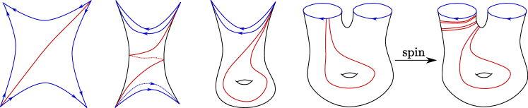
Figure 4: The orientations on the boundary of $\partial\Sigma$ indicates the direction of positive exponential growth. So the ends of the red isolated leaf are required to travel in the negative direction against these arrows.

The reader should consult Figure 4 throughout the rest of the proof. In case (1), $\Sigma$ is a $2m$-gon, and it is easy to find an isolated leaf $\ell$ with the desired properties. In the annular case (2), note that since $\lambda$ is minimal, both crowns must have a positive, even number of spikes. In this case, it is similarly straight forward to find such an isolated leaf.

In case (3), if there is a non-compact crown of $\Sigma$, then we can find a properly embedded oriented arc $\alpha$ in $\Sigma$ with endpoints exiting a spike on the same crown with that is not properly homotopic into $\partial\Sigma$. The geodesic realization of $\alpha$ in $\Sigma$ is the geodesic that we are after. Otherwise, we can similarly find a simple, oriented arc joining a boundary component to itself that is not homotopic rel $\partial\Sigma$ into $\partial\Sigma$. A “spinning” construction then produces the desired isolated leaf. More precisely, the Hausdorff limit of geodesic realizations of segments joining $\partial\Sigma$ to itself in the same homotopy class that wrap more and more around that component of $\partial\Sigma$ is the geodesic we are after; see [Thu22] for details about the spinning construction.

This completes the proof of the Theorem. ∎

4.2 Equivariant transverse measures

From a flow equivariant measure as in Definition 4.1, we would like to extract a transverse measure satisfying a certain equivariance condition. To a $C^{1}$ embedded arc $k\subset X$ transverse to a geodesic lamination $\lambda$, let $\widehat{k}$ be the full preimage in $T^{1}X$ of $k$ minus those directions tangent to $k$ (thus $\widehat{k}$ is two rectangles whose closure is an annulus).

We will often consider oriented arcs. An orientation on $k$ determines a local co-orientation on the leaves of $\lambda$ that it crosses. If $k$ is oriented, we denote by $\widehat{k}^{+}$ the component of $\widehat{k}$ whose geodesic trajectories make positive co-orientation with $k$ and similarly define $\widehat{k}^{-}$.

Definition 4.12.

Let $\lambda$ be a lamination on $X$ and $k$ an oriented arc transverse to $\lambda$. For $x\in k\cap\lambda$, let $\mathfrak{o}(x)\in T^{1}X|_{x}$ be the positively oriented pre-image of $x$ in $\widehat{\lambda}\cap\widehat{k}^{+}$.

By Lemma 2.4, $\mathfrak{o}$ is bi-Lipschitz onto its image in $\widehat{k}^{+}$.

Definition 4.13.

A $(g,G)$-equivariant transverse measure $\mu$ with support a geodesic lamination $\lambda\subset X$ is an assignment to each unoriented arc $k$ transverse to $\lambda$ a finite positive Borel measure $\mu_{k}$ with support equal to $k\cap\lambda$ satisfying the following $(g,G)$-equivariance and compatibility conditions:

• If $k^{\prime}\subset k$, then the pushforward of $\mu_{k^{\prime}}$ under inclusion $k^{\prime}\to k$ is equal to the restriction of $\mu_{k}$ to $k^{\prime}$.

• Give $k$ an orientation. Suppose $k^{\prime}$ is homotopic to $k$ by a homotopy $H$ transverse to $\lambda$ and

  $$k^{\prime}\cap\lambda=\{\pi(g_{t(x)}\mathfrak{o}(x)):x\in k\cap\lambda\}.$$

  Then

  $$dH^{-1}_{*}\mu_{k^{\prime}}=G(\mathfrak{o}(\cdot),t(\cdot))d\mu_{k},$$

  where $H:k\to k^{\prime}$ is induced by the homotopy.

The collection of equivariant transverse measures is denoted by $\mathcal{ML}(X)^{G}$; it is equipped with the following topology: $\mu_{n}\to\mu$ if for all arcs $k$ transverse to $\operatorname{supp}\mu$, $\left(\mu_{n}\right)_{k}\to\mu_{k}$ weak-$*$ on $k$.

Remark 4.14.

If $G$ were constant, as in the case of a Fuchsian representation, Definition 4.13 recovers the usual definition of an invariant transverse measure.

We will now describe a continuous map

$$\mathcal{ML}(T^{1}X)^{G}\to\mathcal{ML}(X)^{G}.$$

The procedure will essentially be by local disintegration.

Let $\nu\in\mathcal{ML}(T^{1}X)^{G}$ and $k$ be an oriented arc transverse to $\lambda=\pi(\operatorname{supp}\nu)$. Consider the measurable functions $r_{+}:\widehat{k}^{+}\to\mathbb{R}_{>0}\cup\{+\infty\}$ and $r_{-}:\widehat{k}^{+}\to\mathbb{R}_{<0}\cup\{-\infty\}$ recording the first return to time to $\widehat{k}^{+}$, in $+$-time and $-$-time, i.e., if $r_{+}(p)<+\infty$, then $g_{r_{+}(p)}p\in\widehat{k}^{+}$, but $g_{t}p\not\in\widehat{k}^{+}$ for all $t\in(0,r_{+}(p))$ and similarly $g_{r_{-}(p)}p\in\widehat{k}^{+}$ but $g_{t}p\not\in\widehat{k}^{+}$ for all $t\in(r_{-}(p),0)$.

There is a $\nu$-a.e. defined measurable projection

$$\pi_{\widehat{k}^{+}}:T^{1}X\to\widehat{k}^{+}$$

by the rule $\pi_{\widehat{k}^{+}}(g_{t}p)=p$ for all $t\in(r_{-}(p)/2,r_{+}(p)/2)$.

For (small) $t>0$ consider the flow box

$$B(t,\widehat{k}^{+}):=\bigcup_{s\in[-t,t]}g_{s}\widehat{k}^{+}\subset T^{1}X,$$

and measures

$$\mu_{\widehat{k}^{+}}^{t}:=\frac{1}{2t}\left(\pi_{\widehat{k}^{+}}\right)_{*}\nu|_{B(t,\widehat{k}^{+})}$$

on $\widehat{k}^{+}$.

Lemma 4.15.

For each small enough $t$, $\mu_{k}^{t}=\pi_{*}\mu_{\widehat{k}^{+}}^{t}$ is a finite Borel measure on $k$. If $k$ meets $\lambda$ non-trivially, then $\mu_{k}^{t}$ converge weak-$*$ to a non-zero measure $\mu_{k}$ as $t\to 0$. Moreover, $\mu_{k}$ does not depend on the choice of orientation on $k$.

Proof.

We invoke the Disintegration Theorem which gives us a measure $\eta_{k}$ on $\widehat{k}^{+}$ satisfying

$$\nu=\int_{p\in\widehat{k}^{+}}\left(\int_{r_{-}(p)/2}^{r_{+}(p)/2}G(p,t)\delta_{g_{t}p}~{}dt\right)d\eta_{k}(p).$$ (12)

Formally, disintegration gives us a Borel family of measures $\nu_{p}\in\mathcal{M}(T^{1}X)$ supported on $\pi_{\widehat{k}^{+}}^{-1}(p)$, each defined up to scale. But the $(g,G)$-equivariance of $\nu$ can be used to show that $\nu_{p}$ is a constant multiple of $\int_{r_{-}(p)/2}^{r_{+}(p)/2}G(p,t)\delta_{g_{t}p}~{}dt$, and we choose the scale factor on each fiber making (12) hold true for some Borel measure $\eta_{k}$ on $\widehat{k}^{+}$ supported on $\widehat{k}^{+}\cap\widehat{\lambda}$.

Let $f$ be a continuous function on $k$ and let $\bar{f}$ be the continuous function on $\widehat{k}^{+}$ obtained by pulling back via $\pi$. Then

$$\left|\int f~{}d\mu_{k}^{t}\right|=\left|\int\bar{f}~{}d\mu_{\widehat{k}^{+}}^{t}\right|\leq\frac{1}{2t}\int_{p\in\widehat{k}^{+}}\left(\int_{-t}^{t}|G(p,s)\bar{f}(p)|~{}ds\right)d\eta_{k}(p)\leq\|f\|_{\infty}\left(\sup_{s\in[-t,t]}\|G(\cdot,s)\|_{\infty}\eta_{k}(\widehat{k}^{+})\right),$$

which proves that $\mu_{k}^{t}$ is a bounded linear operator on $C(k)$, hence is a Borel measure.

Since $G(\cdot,t)$ tends uniformly to $1$ as $t\to 0$, a similar computation shows that $\lim_{t\to 0}\mu_{\widehat{k}}^{t}=\eta_{k}$. Setting $\mu_{\widehat{k}}=\eta_{k}$ completes the proof of convergence of $\mu_{k}^{t}\to\mu_{k}$. That $\mu_{k}$ is independent of the chosen orientation of $k$ is a tedious computation but follows from the symmetries of $\nu$, $G$, and of the construction of $\mu_{\widehat{k}^{+}}^{t}$ under the antipodal involution of $T^{1}X$. ∎

Now that we have extracted a measure $\mu_{k}$ on $k$, we would like to know that it is $(g,G)$-equivariant.

Lemma 4.16.

Let $k$ be an arc transverse to $\lambda=\pi(\operatorname{supp}\nu)$, and let $t\in\mathbb{R}$. Give $k$ an orientation so that $\mathfrak{o}:k\rightarrow\widehat{k}^{+}$ is $\nu$-almost everywhere defined and suppose $k^{\prime}$ differs from $k$ by a homotopy $H:I\times k\to X$ through transverse arcs satisfying $H(s,x)=\pi(g_{st}\mathfrak{o}(x))$ for all $x\in k\cap\lambda$ and $s\in[0,1]$. Then

$$dH^{-1}_{*}\mu_{k^{\prime}}=G(\mathfrak{o}(\cdot),t)d\mu_{k}.$$

Proof.

One checks from the definitions that

$$\pi_{\widehat{k}^{\prime+}}=g_{t}\circ\pi_{\widehat{k}^{+}}\circ g_{-t},~{}\nu\text{-a.e.}$$

Then

$$\mu_{\widehat{k}^{\prime+}}^{s}=\frac{1}{2s}(g_{t}\circ\pi_{\widehat{k}^{+}}\circ g_{-t})_{*}\nu|_{B(s,\widehat{k}^{\prime+})}=\frac{1}{2s}H_{*}(\pi_{\widehat{k}^{+}})_{*}G(\cdot,t)\nu|_{B(s,\widehat{k}^{+})}=H_{*}G(\mathfrak{o}(\cdot),t)\mu_{\widehat{k}^{+}}^{s}.$$

As this equality holds for each $s$ sufficiently small, it is also true in the limit as $s\to 0$ and for the pushforward measures to $k$ and $k^{\prime}$. This completes the proof. ∎

Checking that the second condition in Definition 4.13 holds follows from an approximation argument similar to the previous lemma. That the first condition holds is immediate from the construction.

Proposition 4.17.

The disintegration map $\nu\in\mathcal{ML}(T^{1}X)^{G}\mapsto\{\mu_{k}\}_{k}\in\mathcal{ML}(X)^{G}$ described above is a homeomorphism.

Proof.

That the map is well defined is the content of Lemmas 4.15 and 4.16. Continuity follows along the lines of the proof of Lemma 4.15: $\nu_{n}\to\nu$ if and only if the disintegration over $k$ converges.

Now we construct an inverse mapping. Given $\mu\in\mathcal{ML}(X)^{G}$ with support $\lambda$, consider a transverse arc $k$ equipped with an orientation. The section $x\in k\cap\lambda\to\widehat{x}\in\widehat{k}^{+}$ is bi-Lipschitz onto its image, so the pushforward of $\mu_{k}$ defines a Borel measure $\mu_{\widehat{k}^{+}}$ on $\widehat{k}^{+}$. Extending $\mu_{\widehat{k}^{+}}$ to a $(g,G)$-equivariant measure with support contained in $\widehat{\lambda}$ on $T^{1}X$ is straightforward using (12). Averaging with respect to the antipodal involution produces a flip-invariant and $(g,G)$-equivariant measure $\nu\in\mathcal{ML}(T^{1}X)^{G}$ with support equal to $\widehat{\lambda}$. That this measure did not depend on the choice of $k$ or its orientation can be deduced from the second bullet point (equivariance) in Definition 4.13.

To see that this inverse mapping is continuous, consider a convergent sequence $\mu_{n}\to\mu\in\mathcal{ML}(X)^{G}$ with supports $\lambda_{n}$ and $\lambda$. Call the extended measures $\nu_{n}$ and $\nu\in\mathcal{ML}(T^{1}X)^{G}$ constructed in the previous paragraph. By construction, their supports are $\widehat{\lambda}_{n}$ and $\widehat{\lambda}\subset T^{1}X$.

A sequence $z_{n}\to z$ if and only if every subsequence has a further subsequence converging to $z$. A basic fact from measure theory is that if a sequence of Borel measures $\nu_{n}\to\nu$ weak-$*$ on a compact metric space, then every Hausdorff accumulation point of $\{\operatorname{supp}\nu_{n}\}$ contains $\operatorname{supp}\nu$. So it suffices to consider a subsequence, which we do not rename, with the property that $\lambda_{n}\to\lambda^{\prime}\supset\lambda$ in the Hausdorff topology on closed subsets of $X$. Then also $\widehat{\lambda}_{n}\to\widehat{\lambda}^{\prime}$ in the Hausdorff topology on closed subsets of $T^{1}X$.

Suppose $p_{n}\in\widehat{\lambda}_{n}\cap\widehat{k}^{+}$ converge to $p\in\lambda\cap\widehat{k}^{+}$. Since $G$ is continuous on $T^{1}X\times\mathbb{R}$ and the flow $g_{t}$ is continuous, the measures $\int G(p_{n},t)\delta_{g_{t}p_{n}}~{}dt$ supported on compact segments of leaves of $\widehat{\lambda}_{n}$ converge weak-$*$ on $T^{1}X$ to the corresponding $\int G(p,t)\delta_{g_{t}p}~{}dt$ supported on a compact segment of a leaf of $\widehat{\lambda}$. Since the distributions of the fibers converge (i.e., $(\mu_{n})_{k}\to\mu_{k}$), the extended measures converge weak-$*$ on $T^{1}X$, i.e., $\nu_{n}\to\nu$. This completes the proof. ∎

5 From measures to cocycles and back

In this section, we will make precise the relationship between transverse equivariant measures on laminations defined in Section 4 and the cocycles discussed in Section 3.3.

To define the notion of an equivariant transverse measure, we used the auxiliary data of a norm on the flat bundle $E^{\rho}$ and a parameterization of the geodesic flow on $T^{1}S$ afforded by a hyperbolic metric $X$. This produced a function $G$ describing the expansion of the norm under the geodesic flow (in the subbundle $E^{\rho}_{2}$). Now, Definition 5.2 associates to every element of $\mathcal{ML}(X)^{G}$ an $E^{\rho}$-valued cocycle: an object which is independent of the auxiliary data.

Conversely, in Section 5.2 we extract a transverse $G$-equivariant measure from a cocycle (by way of the bending cocycle of Definition 3.18).

Finally, we establish that these constructions are continuously inverse to one another:

Theorem 5.1.

The space $\mathcal{ML}(X)^{G}$ is homeomorphic to $H^{1}(S,F^{\rho})\setminus\{0\})$ via a map which is homogeneous with respect to positive scale. Consequently, the quotient by positive scale $\mathcal{PML}(X)^{G}$ is a sphere of dimension $6g-7$.

5.1 From measures to cocycles

Let $\eta$ be a coaffine representation with Hitchin linear part, $\rho$. Recall from §3.3 that the top component $\partial\Xi^{+}$ of the convex core boundary is pleated along a $\pi_{1}S$-invariant lamination $\widetilde{\lambda}^{+}$. We choose to work with one component of $\partial\Xi$, though there is a symmetric construction for $\partial\Xi^{-}$.

In the previous Section 4, we made the choice of a norm $\|\cdot\|$ on $E^{\rho}$ and of a hyperbolic metric $X$ on $S$. By $\lambda$, we denote the geodesic straightening of $\lambda^{+}$ on $X$. Lemma 3.19 give us a cocycle $\psi\in Z^{1}(S,E^{\rho})$ satisfying some compatibility properties with respect to $\lambda$. Recall that for an oriented arc $k$ transverse to $\lambda$ on $X$, the function $\mathfrak{o}:k\cap\lambda\to T^{1}X$ from Definition 4.12 is a bi-Lipschitz homeomorphism onto its image and satisfies $\pi\circ\mathfrak{o}(x)=x$.

Using the chosen norm on $E^{\rho}$ and Lemma 2.8, denote by

$$s^{1}:T^{1}X\to E^{\rho}_{2}$$

the unique unit norm positively co-oriented vector in each fiber. This is a Hölder continuous map.

Recall from §2.5 that the bundle $E^{\rho}$ is a pullback of $F^{\rho}\to X$ by $T^{1}X\to X$, so the $\nabla^{\rho}$-parallel transport around the fibers of $T^{1}X\to X$ is trivial. Therefore the parallel transport along $k$ in the integrand below is unambiguous.

Definition 5.2.

Suppose $\mu\in\mathcal{ML}(X)^{G}$ has support $\lambda$. For every oriented arc $k$ transverse to $\lambda$, define a Borel measure on $k$ valued in the fiber $F^{\rho}|_{k(0)}$ by

$$\mu\otimes s^{1}(k)=\mu_{k}\otimes(s^{1}\circ\mathfrak{o})|_{k}.$$

More precisely,

$$\int\mu\otimes s^{1}(k)=\int s^{1}\circ\mathfrak{o}~{}d\mu_{k}=\int_{k}\left(\overline{k_{x}}\right)_{*}s^{1}\circ\mathfrak{o}(x)~{}d\mu_{k}(x)\in F^{\rho}|_{k(0)},$$ (13)

where $k_{x}$ is the parameterized subarc of $k$ begininng at $k(0)$ and ending at $x$ and $\left(\overline{k_{x}}\right)_{*}$ is the $\nabla^{\rho}$-parallel transport.

Then $\mu\otimes s^{1}$ defines an $F^{\rho}$ valued co-chain: $\left(k\mapsto\int\mu\otimes s^{1}(k)\right)$.

Remark 5.3.

Indicator functions on $k^{\prime}\cap\lambda$ are dense in the space of continuous functions on $k\cap\lambda$, where $k^{\prime}$ is a subarc of $k$. Using the restriction property of $\mu\in\mathcal{ML}(X)^{G}$ (Definition 4.13), equation (13) unambiguously defines a bounded linear map from continuous functions on $k$ to $F^{\rho}|_{k(0)}$.

We assert that the cochain described in Definition 5.2 is a cocycle.

Lemma 5.4.

Let $\mu\in\mathcal{ML}(X)^{G}$ with support $\lambda$, and let $k$ and $k^{\prime}$ oriented arcs transverse to $\lambda$ related by a homotopy $H$ through transverse arcs. Then

$$\mu\otimes s^{1}(k^{\prime})=H_{*}(\mu\otimes s^{1}(k)).$$

In particular, $[\mu\otimes s^{1}]\in H^{1}(S,F^{\rho})$.

Proof.

One follows the definitions, in particular see equation (7) and Definition 4.13.

The $G$-equivariance of the sections and the measures exactly cancel; we suppress the arguments of $G$ for readability:

$$H_{*}(\mu_{k}\otimes s^{1}\circ\mathfrak{o}|_{k})=\left(\frac{1}{G\circ H^{-1}}\mu_{k^{\prime}}\right)\otimes\left(G\circ H^{-1}(s^{1}\circ\mathfrak{o})|_{k^{\prime}}\right).$$

It is now straightforward to verify that integrating $\mu\otimes s^{1}$ on oriented transverse arcs is a cocycle. ∎

5.2 From cocycles to measures

From the previous subsection, every equivariant transverse measure defines a cohomology class valued in $F^{\rho}$. Suppose $\eta:\pi_{1}S\to\operatorname{Aff}^{*}(3,\mathbb{R})$ has linear part $\rho$ and bending cocycle $\psi$ with support $\lambda$, as in Definition 3.18. Now we show that $\psi$ is actually equal to integrating some $\mu\otimes s^{1}$ along oriented arcs. The first step is to extract the transverse measure.

Remark 5.5.

In this subsection and the next, we have suppressed the parallel transport along $k$ in the integrals for readability (as in equation (13)). Since this parallel transport operator has bounded operator norm that tends to $1$ on small enough segments, this does not affect our estimates in any meaningful way.

Lemma 5.6.

For every oriented arc $k$ transverse to $\lambda$ on $X$, there is a unique Borel measure $\mu_{k}$ with support equal to $k\cap\lambda$ satisfying

$$\psi(k)=\int_{k}s^{1}\circ\mathfrak{o}~{}d\mu_{k}\in F^{\rho}|_{k(0)}$$

Proof.

We will construct a family of finite Borel measures $\{\vartheta_{\epsilon}\}$ on $k$ with support contained in $k\cap\lambda$ indexed by a positive $\epsilon$ and show that they converge as $\epsilon\to 0$.

Consider the $\epsilon$-neighborhood $\mathcal{N}_{\epsilon}(\lambda)$ on $X$. Then $k\cap\mathcal{N}_{\epsilon}(\lambda)$ is the union of its connected components listed in order along $k$:

$$k\cap\mathcal{N}_{\epsilon}(\lambda)=k_{\epsilon}^{1}\cup...\cup k_{\epsilon}^{m(\epsilon)}.$$

Lemma 2.5 asserts that $\operatorname{diam}(k_{\epsilon}^{i})=O(\epsilon)$ and $m(\epsilon)=O(\log 1/\epsilon)$. Let $x_{\epsilon}^{i}$ denote the initial point of $k_{\epsilon}^{i}$, and define

$$\vartheta_{\epsilon}:=\sum_{i=1}^{m(\epsilon)}\|\psi(k_{\epsilon}^{i})\|_{x_{\epsilon}^{i}}\delta_{x_{\epsilon}^{i}}.$$

Claim 5.7.

If for all oriented subarcs $k^{\prime}\subset k$, it holds that

$$\int_{k^{\prime}}s^{1}\circ\mathfrak{o}~{}d\vartheta_{\epsilon}\to\psi(k^{\prime}),$$

then $\vartheta_{\epsilon}$ converges to a finite Borel measure $\mu_{k}$ as $\epsilon\to 0$.

Proof of Claim 5.7.

Suppose that $\{\vartheta_{\epsilon}\}_{\epsilon>0}$ has two distinct accumulation points $\nu$ and $\nu^{\prime}$. We will show that

$$\int_{k^{\prime}}s^{1}\circ\mathfrak{o}~{}d\nu\not=\int_{k^{\prime}}s^{1}\circ\mathfrak{o}~{}d\nu^{\prime}$$

for some ark $k^{\prime}$, hence at least one of them is not $\psi(k^{\prime})$.

The linear span of indicator functions is dense in $C(k\cap\lambda)$ and $\nu\not=\nu^{\prime}$, so there is a $k^{\prime}$ such that $\nu(k^{\prime})\not=\nu^{\prime}(k^{\prime})$, i.e., that the $\nu$ and $\nu^{\prime}$ integrals of the indicator function on $k^{\prime}$ disagree. Furthermore, we may find such a $k^{\prime}$ with arbitrarily small diameter.

Consider the integrand

$$s^{1}\circ\mathfrak{o}:k^{\prime}\cap\lambda\to F^{\rho}|_{k^{\prime}(0)}.$$

With respect to a $\|\cdot\|_{k^{\prime}(0)}$-orthonormal basis $e_{1},e_{2},e_{3}$ with $\langle e_{2}\rangle=E_{2}^{\rho}|_{k^{\prime}(0)}$, we have

$$s^{1}\circ\mathfrak{o}=f_{1}e_{1}+f_{2}e_{2}+f_{3}e_{3},$$

where $f_{i}:k\cap\lambda\to\mathbb{R}$ are $\alpha$-Hölder continuous (see Lemma 2.8). Thus

$$\left\|\int_{k^{\prime}}s^{1}\circ\mathfrak{o}~{}d(\nu-\nu^{\prime})\right\|^{2}=\sum_{i=1}^{3}\left|\int_{k^{\prime}}f_{i}~{}d(\nu-\nu^{\prime})\right|^{2}.$$

Corollary 3.21 implies that

$$|f_{2}-1|=O(\operatorname{diam}(k^{\prime})^{\alpha})\text{ and }|f_{i}|=O(\operatorname{diam}(k^{\prime})^{\alpha})\text{ for $i=1,3$}.$$

Hence that

$$\left\|\int_{k^{\prime}}s^{1}\circ\mathfrak{o}~{}d(\nu-\nu^{\prime})\right\|^{2}\geq\left|\int_{k^{\prime}}f_{2}~{}d(\nu-\nu^{\prime})\right|^{2}-(\nu(k^{\prime})-\nu^{\prime}(k^{\prime}))^{2}O(\operatorname{diam}(k^{\prime})^{2\alpha}).$$

Furthermore, we obtain

$$\left|\int_{k^{\prime}}f_{2}d(\nu-\nu^{\prime})\right|^{2}\geq[(1-O(\operatorname{diam}(k^{\prime})^{\alpha})(\nu(k^{\prime})-\nu^{\prime}(k^{\prime}))]^{2}.$$

All together this gives

$$\left\|\int_{k^{\prime}}s^{1}\circ\mathfrak{o}~{}d(\nu-\nu^{\prime})\right\|^{2}\geq(\nu(k^{\prime})-\nu^{\prime}(k^{\prime}))^{2}(1-O(\operatorname{diam}(k^{\prime})^{2\alpha})).$$

Thus, if $\operatorname{diam}(k^{\prime})$ is small enough, then this quantity is positive because $\nu(k^{\prime})\not=\nu^{\prime}(k^{\prime})$, which completes the proof of the claim. ∎

It remains to prove that the hypothesis of Claim 5.7 holds. We will prove that

$$\int_{k}s^{1}\circ\mathfrak{o}~{}d\vartheta_{\epsilon}\to\psi(k).$$

The proof that the analogous claim also holds for all subarcs $k^{\prime}\subset k$ is identical.

Repeated application of the cocycle property of $\psi$ and that its support is $\lambda$ (in the sense of Lemma 3.19) gives

$$\psi(k)=\sum_{i=1}^{m(\epsilon)}\psi(k_{\epsilon}^{i}),$$

while

$$\int_{k}s^{1}\circ\mathfrak{o}~{}d\vartheta_{\epsilon}=\sum_{i=1}^{m(\epsilon)}s^{1}\circ\mathfrak{o}(x_{\epsilon}^{i})\|\psi(k_{\epsilon}^{i})\|.$$

Corollary 3.21 implies that there is a uniform bound on $\left\|\psi(k_{\epsilon}^{i})\right\|$ and that

$$\left\|\psi(k_{\epsilon}^{i})-\|\psi(k_{\epsilon}^{i})\|s^{1}\circ\mathfrak{o}(x_{\epsilon}^{i})\right\|=O(\operatorname{diam}(k_{\epsilon}^{i})^{\alpha})=O(\epsilon^{\alpha})$$

for all $i$.

Therefore,

$$\left\|\psi(k)-\int_{k}s^{1}\circ\mathfrak{o}~{}d\vartheta_{\epsilon}\right\| \leq\sum_{i=1}^{m(\epsilon)}\left\|\psi(k_{\epsilon}^{i})-\|\psi(k_{\epsilon}^{i})\|s^{1}\circ\mathfrak{o}(x_{\epsilon}^{i})\right\|$$

$$\leq m(\epsilon)O(\epsilon^{\alpha})=O(\epsilon^{\alpha}\log 1/\epsilon),$$

which tends to $0$ with $\epsilon$. This completes the proof of the Lemma. ∎

Lemma 5.8.

The assignment $\left(k\mapsto\mu_{k}\right)$ from Lemma 5.6 defines an element of $\mathcal{ML}(X)^{G}$ with support $\lambda$.

Proof.

Let $k$ and $k^{\prime}$ be transverse arcs related by a homotopy $H$. Lemma 5.6 gives

$$\psi(k^{\prime})=\int s^{1}~{}d\mu_{k^{\prime}}\text{ and }\psi(k)=\int s^{1}~{}d\mu_{k}.$$

Since $\psi$ is a cocycle, we have

$$H_{*}(\psi(k))=\psi(k^{\prime}).$$

We compute

$$H_{*}(\psi(k))=\int_{k^{\prime}}(H_{*}s^{1})~{}dH_{*}\mu_{k}=\int_{k^{\prime}}s^{1}~{}(G\circ H^{-1})dH_{*}\mu_{k}.$$

Thus

$$\int_{k^{\prime}}s^{1}~{}d\mu_{k^{\prime}}=\int_{k^{\prime}}s^{1}~{}(G\circ H^{-1})dH_{*}\mu_{k}$$

A similar computation holds on every pair of subarcs (which are homotopic by $H$). Therefore the two measures agree on the indicator functions of subarcs, which are dense in the space of continuous functions on $\lambda\cap k$. So as Borel measures

$$dH^{-1}_{*}\mu_{k^{\prime}}=G(\mathfrak{o}(\cdot),t(\cdot))d\mu_{k}$$

as required. ∎

Lemmas 5.6 and 5.8 show that there is a well defined map

$$\Psi:\{\eta:\pi_{1}S\to\operatorname{Aff}^{*}(3,\mathbb{R})\text{ with linear part $\rho$}\}/\operatorname{TAff}^{*}(3,\mathbb{R})\to\mathcal{ML}(X)^{G}.$$

5.3 $\Phi$ is a homeomorphism

Lemma 5.4 shows that there is a well-defined map

$$\Phi:\mathcal{ML}(X)^{G} \to H^{1}(S,F^{\rho})\setminus\{0\}$$ (14)

$$\mu \mapsto[\mu\otimes s^{1}]$$ (15)

Lemma 5.9.

The map $\Phi$ is a bijection.

Proof.

The inverse map is given as the composition of $\Psi$ with the map from Lemma 3.4 sending a cohomology class $\varphi$ to the bending cocycle $\psi(\eta_{\varphi})$ (Definition 3.18). ∎

We now demonstrate that the map $\mu\mapsto[\mu\otimes s^{1}]$ respects the topology of the two spaces.

Proposition 5.10.

The map $\Phi$ is continuous and homogeneous with respect to positive scale.

Proof.

Consider a convergent sequence $\mu_{n}\to\mu\in\mathcal{ML}(X)^{G}$ with supports denoted by $\lambda_{n}=\operatorname{supp}\mu_{n}$ and $\lambda=\operatorname{supp}\mu$. As in the proof of Proposition 4.17, every Hausdorff accumulation of $\lambda_{n}$ contains $\lambda$. Passing to a subsequence, we assume that $\lambda_{n}$ converges Hausdorff to some $\lambda^{\prime}\supset\lambda$.

Every small enough oriented arc $k$ meeting $\lambda^{\prime}$ transversely meets $\lambda_{n}$ transversely for $n$-large enough. For each $n$, let $\mathfrak{o}_{n}:k\cap\lambda_{n}\rightarrow\widehat{k}$ be the positively co-orientation lift, and $\mathfrak{o}$ similarly defined for $\lambda$. Denote by $\vartheta_{n}=\left(\mu_{n}\right)_{k}$, and $\vartheta=\mu_{k}$. By definition of the topology on $\mathcal{ML}(X)^{G}$, $\vartheta_{n}\to\vartheta$ weak-$*$ as $n\to\infty$.

Defining

$$I_{n}=\int_{k}s^{1}\circ\mathfrak{o}_{n}~{}d\vartheta_{n}\text{ and }I=\int_{k}s^{1}\circ\mathfrak{o}~{}d\vartheta,$$

our goal is to show that $I_{n}\to I$ as $n\to\infty$.

For $\delta>0$, we have $\lambda\subset\mathcal{N}_{\delta}(\lambda^{\prime})$ and $\lambda_{n}\subset\mathcal{N}_{\delta}(\lambda^{\prime})$ for all $n$ large enough. In particular, $\mathcal{N}_{\delta}(\lambda^{\prime})\cap k\supset\lambda\cap k$ and $\mathcal{N}_{\delta}(\lambda^{\prime})\cap k\supset\lambda_{n}\cap k$ for all $n$ large enough. By Lemma 2.5, $\mathcal{N}_{\delta}(\lambda^{\prime})\cap k$ consists of intervals $k^{1},...,k^{m(\delta)}$, each of diameter $O(\delta)$.

Choose points $x^{i}\in\lambda^{\prime}\cap k^{i}$ and define

$$R=\sum_{i=1}^{m(\delta)}s^{1}(\mathfrak{o}(x^{i}))\vartheta(k^{i}).$$

Choose also $x_{n}^{i}\in\lambda_{n}\cap k^{i}$ converging to $x^{i}$ as $n\to\infty$, and define

$$R_{n}=\sum_{i=1}^{m(\delta)}s^{1}(\mathfrak{o}_{n}(x_{n}^{i}))\vartheta_{n}(k^{i}).$$

Each map

$$x\in\lambda_{n}\cap k\mapsto s^{1}(\mathfrak{o}_{n}(x))\in E_{2}^{\rho}\text{ and }x\in\lambda\cap k\mapsto s^{1}(\mathfrak{o}(x))\in E_{2}^{\rho}$$

is $\alpha$-Hölder with uniformly bounded $\alpha$-Hölder norm. Using this, we estimate

$$\left\|I_{n}-R_{n}\right\|\leq\sum_{i=1}^{m(\delta)}\int_{k^{i}}\left\|s^{1}(\mathfrak{o}_{n}(x))-s^{1}(\mathfrak{o}_{n}(x_{n}^{i}))\right\|~{}d\vartheta_{n}(x)=O(\delta^{\alpha})\vartheta_{n}(k),$$

and similarly

$$\left\|I-R\right\|=O(\delta^{\alpha})\vartheta(k).$$

The triangle inequality and $\vartheta_{n}(k)\to\vartheta(k)$ give that

$$\|I-I_{n}\|\leq O(\delta^{\alpha})(\vartheta_{n}(k)+\vartheta(k))+\|R_{n}-R\|=O(\delta^{\alpha})+\|R_{n}-R\|.$$

Given $\epsilon>0$, we can choose $\delta$ such that $O(\delta^{\alpha})<\epsilon/2$.

Now that $\delta$ is fixed, we bound

$$\|R_{n}-R\| \leq\sum_{i=1}^{m(\delta)}\left\|s^{1}(\mathfrak{o}_{n}(x_{n}^{i}))\vartheta_{n}(k^{i})-s^{1}(\mathfrak{o}(x^{i}))\vartheta(k^{i})\right\|$$ (16)

using the general fact that $|xy-zw|\leq|y|\cdot|x-z|+|z|\cdot|w-y|$:

By Hausdorff convergence of $\widehat{\lambda}_{n}\to\widehat{\lambda}^{\prime}$, by our choice of $x_{n}^{i}\to x^{i}$, and by continuity of $s^{1}$, for any $\epsilon^{\prime}>0$,

$$\left\|s^{1}(\mathfrak{o}_{n}(x_{n}^{i}))-s^{1}(\mathfrak{o}(x^{i}))\right\|<\epsilon^{\prime}$$

for large enough $n$. By weak-$*$ convergence of $\vartheta_{n}\to\vartheta$, and because $k^{i}$ is a continuity set for $\vartheta$ (since $\partial k^{i}$ does not meet $\lambda^{\prime}$) we have

$$|\vartheta_{n}(k^{i})-\vartheta(k^{i})|<\epsilon^{\prime}$$

for $n$ large enough.

Since $\vartheta(k^{i})\leq\vartheta(k)$, we obtain

$$\|R_{n}-R\|\leq m(\delta)\left(\vartheta(k)\epsilon^{\prime}+\|s^{1}\circ\mathfrak{o}\|_{\infty}\epsilon^{\prime}\right)$$

for all $n$ large enough. In particular, since $\delta$ is already fixed, we can take $\epsilon^{\prime}$ small enough and then $n$ suitably large so that $\|R_{n}-R\|<\epsilon/2$ holds.

This proves that if $n$ is large enough then $\|I_{n}-I\|$ is smaller than $\epsilon$. Since $\epsilon$ was arbitrary, we have proved that $I_{n}\to I$. Since $k$ was arbitrary, continuity of $\Phi$ follows.

That $\Phi$ is homogeneous follows from the definitions. This completes the proof. ∎

Although the function $G$ depended on the choices of a parametrization of the flow $g_{t}$ and a norm $\|\cdot\|$ on $E^{\rho}$, Lemma 5.9 demonstrates that the resulting space of equivariant measures does not, in the sense that $\Phi$ is canonical; it identifies $\mathcal{ML}(X)^{G}$ with a cohomology theory defined independently of any choices.

Proof of Theorem 5.1.

Lemma 5.9 gives that $\Phi$ is bijective, while Proposition 5.10 states that $\Phi$ is continuous and homogeneous with respect to positive scale. We obtain an induced bijective continuous mapping

$$\mathcal{PML}(X)^{G}\to\mathbb{P}_{>0}(H^{1}(S,F^{\rho})\setminus\{0\})\cong\mathbb{S}^{6g-7}.$$

Because $\mathcal{PML}(X)^{G}$ can be identified with a closed subset of probability measures on $T^{1}X$ (Proposition 4.17) which is compact in the weak-$*$ topology, and $\mathbb{S}^{6g-7}$ is Hausdorff, this mapping is a homeomorphism. This completes the Theorem. ∎

6 Flat vector bundles over geodesic laminations

Let $\rho:\pi_{1}S\to\operatorname{SL}(3,\mathbb{R})$ be a Hitchin representation. Recall the flow-invariant Hölder continuous Anosov splitting $E^{\rho}=E_{1}\oplus E_{2}\oplus E_{3}$ over $T^{1}X$ from §2.5. The involution $p\mapsto\overline{p}$ preserves the $E_{2}$ subbundle, while permuting $E_{1}$ and $E_{3}$. Since $E^{\rho}$ was constructed as a pullback of $F^{\rho}$ by the tangent projection, $E_{2}|_{p}$ is naturally identified with $E_{2}|_{\overline{p}}$. Therefore, $E_{2}$ descends to a line bundle $\overline{E_{2}}$ over $\mathbb{P}TX$.

Let $\lambda\subset S$ be a geodesic lamination.

Definition 6.1.

Let $F_{2}^{\rho}(\lambda)=F_{2}\to\lambda$ be the pullback of $\overline{E_{2}}$ by the inclusion $\lambda\cong\mathbb{P}T\lambda\hookrightarrow\mathbb{P}TX$. The flat connection $\nabla^{\rho}$ restricts to a flat connection along the leaves of $\lambda$.

Although $\overline{E_{2}}$ need not be flat, we will nevertheless produce a flat connection on $F_{2}^{\rho}(\lambda)$. Indeed, the goal of this section is to show that there is a natural Hölder extension of the connection $\nabla^{\rho}$ to a Hölder flat connection on $F_{2}\to\lambda$. First, we formalize the notion of a flat connection on a vector bundle over a lamination compatible with a given connection along the leaves (Definition 6.7), which gives a way to extend parallel transport in directions transverse to the leaves.

The slithering map studied in [BD17] furnishes the bundle $F_{2}$ with a flat connection in this sense (Lemma 6.15), and we obtain the main theorem of the section as a corollary.

Theorem 6.2.

For any Hitchin representation $\rho:\pi_{1}S\to\operatorname{SL}(3,\mathbb{R})$ and any geodesic lamination $\lambda\subset S$ the bundle $F_{2}\to\lambda$ has a Hölder continuous flat connection $\nabla$, called the slithering connection, which is compatible with $\nabla^{\rho}$ along the leaves of $\lambda$.

From the formalism developed in Section §6.1, we extract a combinatorial description of flat bundles over a connected lamination in terms of a snug train track that carries $\lambda$. In particular, suppose that $\mathcal{N}$ is a snug train track neighborhood for $\lambda$ equipped with a foliation by ties with quotient $q:\mathcal{N}\to\tau$ (see §2.3).

Proposition 6.3.

There is a character $\chi:\pi_{1}\tau\to\mathbb{R}^{\times}$ defining a flat bundle $F_{\chi}\to\tau$

$$F_{\chi}=(\widetilde{\tau}\times\mathbb{R})/\left[(x,v)\sim(\gamma.x,\chi(\gamma)v)\right]$$

such that $F_{2}\to\lambda$ is isomorphic to the pullback of $F_{\chi}$ by $q$.

Thus over each connected component of a lamination $\lambda$, the bundle $F_{2}$ is determined by a finite collection of data which can be encoded as a train track with holonomy.

Remark 6.4.

The results in this section have analogues for $E_{i}|_{\widehat{\lambda}}$, $i=1,\dots 3$ as well as for Borel Anosov representations into $\operatorname{SL}(d,\mathbb{R})$. The proofs require no significant changes.

6.1 Train tracks and flat connections

In the rest of this section, we will be interested in connected geodesic lamination $\mu\subset\mathcal{M}$, where $\mathcal{M}$ is a train track neighborhood of $\mu$ equipped with a foliation by ties. The leaf space of the foliation of $\mathcal{M}$ by its ties $\theta=\mathcal{M}/\sim$ is a train track carrying $\mu$. See §2.3 for terminology.

Remark 6.5.

We treat real vector bundles of arbitrary finite dimension over a lamination, though we will only use the case when the dimension is one. The one-dimensional case is slightly simpler, as the difference between the vector bundle and its frame bundle essentially disappears.

Definition 6.6 (Flat vector bundle over a lamination).

A (finite-dimensional real) flat vector bundle $\zeta:E\to\mu$ is a finite-dimensional vector bundle equipped with an atlas

$$\mathcal{A}=\{\psi_{\alpha}:\zeta^{-1}(U_{\alpha})\to U_{\alpha}\times\mathbb{R}^{d}\}$$

of vector bundle charts where the linear part of the transition maps is constant, i.e., $\psi_{\beta}\circ\psi_{\alpha}^{-1}(p,v)=(\phi_{\beta\alpha}(p),A_{\beta\alpha}v)$, where $\phi_{\beta\alpha}$ is a homeomorphism (where defined) and $A_{\beta\alpha}\in\operatorname{GL}(\mathbb{R}^{d})$ is independent of $p$.

Associated to such a vector bundle is the frame bundle

$$\zeta_{\mathcal{B}}:\mathcal{B}(E)\to\mu,$$

the fiber of which at $p$ is the set of ordered bases of $E|_{p}$. The atlas of $E$ gives an atlas of charts for $\mathcal{B}(E)$ with image in $U_{\alpha}\times\mathcal{B}(\mathbb{R}^{d})$.

The local sections of $\zeta_{\mathcal{B}}$ that are constant in charts are called the local flat frames of $E$. A local section $s_{1}$ of $E$ is flat if there exist local sections $s_{2},\dots,s_{d}$ on the same neighborhood in $\mu$ so that $(s_{1},\dots,s_{d})$ is a local flat frame (i.e. $s_{1}$ is flat when it can be extended to a flat frame).

It is an exercise to check that given a point $(p,v)\in E$, there exists exactly one local flat section $s$ of $E$ so that $s(p)=v$ (up to extending and restricting the neighborhood on which $s$ is defined).

Suppose $E$ is a vector bundle over a space with a Hölder class of metrics. A Hölder structure on $E$ is an atlas of charts such that the transition maps $\phi_{\beta\alpha}$ are Hölder functions into $\operatorname{GL}(d,\mathbb{R})$; a flat structure on $E$ is compatible with a Hölder structure if its flat sections are Hölder.

We may also approach flatness from the perspective of flat connections. Let $\zeta:E\to\mu$ be an $\mathbb{R}^{d}$-bundle over $\mu$, which is not necessarily flat. Let $\nabla^{0}$ be a flat connection along the leaves of $\mu$: for every leaf $l$ of $\mu$, $\nabla^{0}$ is a flat connection on the bundle $E|_{l}=\zeta^{-1}(l)$, the restriction of $E$ to $l$.

To an embedded $C^{1}$ path $\alpha\subset\mathcal{M}$ transverse to $\mu$, denote by $T_{\alpha}=\alpha\cap\mu$ the transversal space of $\mu$ in $\alpha$. If $\zeta:E\to\mu$ is an $\mathbb{R}^{d}$-bundle, then $E|_{\alpha}$ is shorthand notation for the bundle $E$ restricted to $T_{\alpha}$.

Definition 6.7.

[Flat connection] Let $\mu$ be a lamination in a train track neighborhood $\mathcal{M}$. A flat connection $\nabla$ on $\zeta:E\to\mu$ extending a flat connection $\nabla^{0}$ along the leaves of $\mu$ is an assignment

$$\nabla:\alpha\in\{\text{embedded transversals to $\mu$ in $\mathcal{M}$}\}\mapsto\nabla_{\alpha}\in\{\textrm{continuous sections}~{}T_{\alpha}\rightarrow\mathcal{B}(E)|_{\alpha}\}/\operatorname{GL}(d,\mathbb{R}).$$

Here $\operatorname{GL}(d,\mathbb{R})$ is acting on the fibers of $E|_{\alpha}$ via a trivialization. The map $\nabla$ is required to satisfy

1. Restriction. If $\alpha^{\prime}\subset\alpha$ then

   $$\nabla_{\alpha^{\prime}}=(\nabla_{\alpha})|_{\alpha^{\prime}}.$$

2. Compatibility with $\nabla^{0}$. Suppose $\alpha$ and $\beta$ are transversely isotopic via $H$, Then $\nabla$ satisfies

   $$H_{*}\circ\nabla_{\alpha}=\nabla_{\beta}$$

   (i.e. along leaves, $\nabla$ restricts to $\nabla^{0}$). Here $H_{*}$ denotes $\nabla^{0}$-parallel transport along leaves parameterized by $H$.

The local flat sections of $\mathcal{B}(E)$ defining $\nabla$ are called the local flat frames of $E$, the components of which are called the local flat sections of $E$. We will denote by $X_{*}(v)$ the flat extension of a vector $v$ along a suitable subset $X$ by $\nabla$.

The connection $\nabla^{0}$ is part of the data of $\nabla$, so that $\nabla$ may be used to parallel transport vectors along the leaves. of $\mu$. To prove the following lemma, one necessarily defines $\nabla$ as the $\operatorname{GL}(d,\mathbb{R})$-classes of local flat sections of the frame bundle $\mathcal{B}(E)$.

Lemma 6.8.

A flat vector bundle $\zeta:E\to\mu$ admits a unique flat connection $\nabla$ which is compatible in the sense that the local flat sections of $\zeta$ are equal to the local flat sections of $\nabla$.

Given a train track neighborhood $\mathcal{M}$ of $\mu$, and a flat connection $\nabla$ on a bundle $E$ over $\mu$, the following result is a useful consequence of the second item in Definition 6.7. For a point $p$ on a lamination $\mu$ carried by a traintrack $\mathcal{M}$, denote by $\ell(p)$ and $t(p)$ the leaf of $\lambda$ and the tie of $\mathcal{M}$ containing $p$, respectively.

Lemma 6.9.

Let $(p,v)\in E$, and suppose $q\in\mu$ is such that $\ell(p)$, $t(q)$, $\ell(q)$, and $t(p)$ bound a rectangle embedded in $\mathcal{M}$ whose sides are labelled (respectively) $L_{p},S_{q},L_{q},S_{p}$. Then the $\nabla$-parallel transport around this rectangle is trivial, i.e.

$$(L_{q})_{*}\circ(S_{p})_{*}(v)=(S_{q})_{*}\circ(L_{p})_{*}(v).$$

Proof.

We recognize the fact that the rectangle is the image of the boundary of a homotopy between $t(p)$ and $t(q)$, and apply the property from the definition of $\nabla$:

$$(H)_{*}\circ\nabla_{t(p)}=\nabla_{t(q)}.$$

Consider the local flat section $\operatorname{im}(H)_{*}(v)$. The restriction of this section to $t(p)\cup\ell(q)$ and $\ell(p)\cup t(q)$ are exactly

$$(L_{q})_{*}\circ(S_{p})_{*}(v)$$

and

$$(S_{q})_{*}\circ(L_{p})_{*}(v),$$

respectively. We conclude that the Lemma holds because $H_{*}(v)$ is well-defined. ∎

Remark 6.10.

The same proof holds more generally for arbitrary pairs of homotopic embedded transversals. In particular, a flat connection $\nabla$ on $\mu$ extending $\nabla^{0}$ is determined locally by its flat sections over a tie.

Recall that collapsing the ties of $\mathcal{M}$ induces a map $q:\mathcal{M}\to\theta$ which is $C^{1}$ restricted to the leaves of $\mu$. We define branch charts for the bundle $E$ in the presence of $\theta$ as follows. Let $U_{b}=q^{-1}(b)$, where $b$ is a branch of $\theta$, and let $V_{b}$ be the pre-image in $E$ of $U_{b}$. Let $T_{b}$ be the transversal space of $U_{b}$, i.e., the space of leaves of $\mu$ running through $U_{b}$.

Given a flat connection $\nabla$ extending $\nabla^{0}$ as in Definition 6.7, Lemma 6.9 guarantees the existence of a flat section of the frame bundle $\mathcal{B}(E)|_{U_{b}}$. Let $A_{b}$ be the linear map taking this frame to the standard frame in $\mathbb{R}^{d}$. The branch chart is defined as

$\psi_{b}:V_{b}\to U_{b}\times\mathbb{R}^{d}$

$(p,v)\mapsto\left(\ell(p),t(p),A_{b}v\right).$

A different choice of flat section over $U_{b}$ would effect $A_{b}$ by post-composition with an element of $\operatorname{GL}(d,\mathbb{R})$. Extending the open sets $U_{b}$ slightly over each switch to $U_{b}^{\prime}$ (with pre-images $V_{b}^{\prime}\subset E$), we see that the transitions between branch charts are constant.

Lemma 6.11.

Given a flat connection $\nabla$ on a vector bundle $E$ over a lamination, the atlas (described above)

$$\mathcal{A}(\nabla)=\left\{\psi_{b}:V^{\prime}_{b}\to U_{b}^{\prime}\times\mathbb{R}^{d}\right\}$$

of vector bundle charts is flat.

Proof.

One can construct $U_{b}^{\prime}$ so that the triple-wise intersection of any such distinct charts is trivial, so the cocycle condition on transition maps is trivially satisfied. A pair of adjacent train track charts $U^{\prime}_{b}$ and $U^{\prime}_{b^{\prime}}$ overlap on a small isotopy of a tie. The flat sections $A_{b}$ and $A_{b}^{\prime}$ defining the branch charts differ on their overlap by a constant element of $\operatorname{GL}(d,\mathbb{R})$ (see Lemma 6.9). ∎

Our next objective is to combinatorialize an $\mathbb{R}^{d}$-bundle $\zeta:E\to\mu$ with flat connection $\nabla$ and build a flat $\mathbb{R}^{d}$-bundle over a train track $\theta$ that carries $\mu$. Choosing a point $p\in\theta$ gives a holonomy representation

$$\operatorname{hol}:\pi_{1}(\theta,p)\to\operatorname{GL}(E|_{p})\cong\operatorname{GL}(d,\mathbb{R}),$$

as follows. Each $[\alpha]\in\pi_{1}(\theta,p)$ lifts to a continuous concatenation of segments of leaves in $\lambda$ and segments of ties of $\mathcal{M}$, call it $\alpha$. Then let

$$\operatorname{hol}([\alpha])=\overline{\alpha}_{*}$$

the $\nabla$-parallel transport around $\overline{\alpha}$. Any two choices of such lifts $\alpha$ and $\alpha^{\prime}$ differ by a sequence of rectangles, so that Lemma 6.9 guarantees that $\operatorname{hol}$ is well-defined. This is the usual definition of holonomy.

There is a flat $\mathbb{R}^{d}$-bundle $E^{\operatorname{hol}}$ over $\theta$ constructed by taking $\pi_{1}\theta$-orbits:

$$E^{\operatorname{hol}}=(\widetilde{\theta}\times\mathbb{R}^{d})/\left[(x,v)\sim([\alpha].x,\operatorname{hol}([\alpha])v)\right].$$

The bundle $E^{\operatorname{hol}}$ has a flat connection $\nabla^{\operatorname{hol}}$ obtained by pushing forward the trivial connection on $\mathbb{R}^{d}\times\widetilde{\theta}$ by the quotient projection.

Although $\mu$ does not generally have a reasonable universal cover (it is generally not path connected), using the train track $\theta$, we still recover the following direct analogue of the structure theorem for flat bundles (see, e.g., [Ste51, §13]). Its proof is essentially the content of this section.

Proposition 6.12.

In the category of flat bundles, $q^{*}(E^{\operatorname{hol}},\nabla^{\operatorname{hol}})$ is isomorphic to $(E,\nabla)$.

The proof is no different than in the case of a manifold, though one works in the universal cover of the traintrack neighborhood $\mathcal{M}$. The branch charts give the necessary local trivializations.

6.2 Key examples: Hitchin representations

In this section we apply our general discussion to line bundles coming from Borel-Anosov representations (see §2.5 for definitions). In particular, we obtain Theorem 6.2 and Proposition 6.3. We begin with a brief discussion of the slithering map defined in [BD17] for Borel-Anosov representations.

The limit curves $\xi$ and $\xi^{*}$ from Section 2.5 may be understood as a single map to the space of full flags in $\mathbb{R}^{3}$; call this map $x\mapsto\mathcal{F}(x)$. These flags are transverse: for any distinct $x$ and $y$ in $\partial\pi_{1}S$, $\xi(x)\oplus\xi^{*}(y)=\mathbb{R}^{3}$ is direct [Lab06]. In general, Borel Anosov representations have a transverse limit map to the space of full flags, constructed from the Anosov splitting, see §2.5.

In particular, for any triple of points $x,y,z\in\partial\pi$, the flags $\mathcal{F}(x),\mathcal{F}(y),\mathcal{F}(z)$ are pairwise transverse. It is an exercise in linear algebra that for a pairwise transverse triple of full flags $\mathcal{F}_{1},\mathcal{F}_{2},\mathcal{F}_{3}$ of $\mathbb{R}^{d}$, there exists a unique element $g_{1}^{2,3}\in\operatorname{GL}(d,\mathbb{R})$ which is unipotent, stabilizes $\mathcal{F}_{1}$ and has $g_{1}^{2,3}.\mathcal{F}_{2}=\mathcal{F}_{3}$.

The slithering map is the unique Hölder extension of this map across collections of parallel leaves in a maximal lamination. More precisely, if $g$ and $h$ are oriented leaves in a maximal lamination $\lambda$ which share an endpoint, $g^{-}=h^{-}$, then the slithering map $\Sigma_{hg}$ is the natural isomorphism $\mathbb{R}^{d}\rightarrow\mathbb{R}^{d}$ which acts trivially on $\mathcal{F}(g^{-})$ and takes $\mathcal{F}(g^{+})\mapsto\mathcal{F}(h^{+})$. Bonahon and Dreyer extended this rule to pairs of coherently oriented geodesics that do not share a common endpoint; this map is called the slithering map

$$(h,g)\mapsto\Sigma_{hg}\in\operatorname{SL}(d,\mathbb{R}).$$

The slithering map obeys a composition rule when a geodesic $g^{\prime}$ separates a pair of geodesics $g$ and $g^{\prime\prime}$. Namely

$$\Sigma_{g^{\prime\prime}g}=\Sigma_{g^{\prime\prime}g^{\prime}}\circ\Sigma_{g^{\prime}g}.$$

It is also independent of the (coherent) orientation of the geodesics:

$$\Sigma_{\overline{g}^{\prime}\overline{g}}=\Sigma_{g^{\prime}g}$$

The assumption that $g^{\prime}$ separates is necessary; generically the slithering map around a triangle is nontrivial. To be precise, if $x,y,z$ are leaves of a lamination forming an ideal triangle, then the composition

$$\Sigma_{xy}\circ\Sigma_{yz}\circ\Sigma_{zx}$$ (17)

is generically not a root of the identity. We direct the reader to Section 5 of [BD17] for the details.

Remark 6.13.

While Bonahon-Dreyer define the slithering map only for maximal laminations, there is an analogous construction for arbitrary laminations; the map $(h,g)\mapsto\Sigma_{hg}$ is only defined when all of the gaps between $g$ and $h$ are bounded by asymptotic leaves. The proof of this fact follows with no adjustments at all.

In particular, when $\mathcal{N}$ is a snug train neighborhood track carrying $\lambda$, then $\Sigma_{hg}$ is defined whenever $h$ and $g$ are joined by a tie of $\widetilde{\mathcal{N}}$; see §2.3.

Given a lamination $\lambda$ on $S$ and an Anosov representation $\rho$, we will use the slithering map to construct a flat connection on the line bundles $F_{2}=F_{2}^{\rho}$ over $\lambda$ (recall Definition 6.1). Flow invariance of the Anosov splitting from §2.5 guarantees that $\nabla^{\rho}$ restricts to a flat connection on $F_{2}|_{\ell}$ for each leaf $\ell\subset\lambda$.

Definition 6.14.

Let $\mathcal{N}$ be any snug train track neighborhood for $\lambda$ equipped with a foliation by ties, and let $t$ be a tie. A non-zero section $\omega:t\to F_{2}|_{t}$ is a slithering section if for all $p,q\in t\cap\lambda$

$$\omega(q)=\Sigma_{\ell(q)\ell(p)}\omega(p)$$

In other words, a slithering section is obtained by extending a non-zero vector over a tie using the slithering map.

Lemma 6.15 (Slithering connection).

The collection of slithering sections define a flat Hölder connection on $F_{2}$ (extending $\nabla^{\rho}$ along the leaves) called the slithering connection.

Proof.

Let $\nabla$ be the local extension of all slithering sections by $\nabla^{\rho}$-parallel transport. Since $F_{2}$ is one-dimensional, non-zero sections are also sections of $\mathcal{B}(F_{2})$. Certainly $\nabla$ satisfies the restriction condition and it is Hölder because the slithering map is.

Over any transversal $t$, there exists a unique slithering section up to scale (because slithering maps are linear). Since $\nabla$ extends $\nabla^{\rho}$ and $\Sigma_{qp}^{\rho}$ depends only on $\ell(q)$ and $\ell(p)$, it follows that for two ties $t$ and $t^{\prime}$ and an isotopy $H$ between them that $H_{*}\circ\nabla_{t}=\nabla_{t^{\prime}}$. ∎

Lemma 6.15 and Proposition 6.12 imply Theorem 6.2 and Proposition 6.3 as corollaries.

7 Affine Laminations

The equivariant transverse measures discussed in §4.2 depended on a choice of norm on $E^{\rho}$. In Section 6 we found that this bundle restricted to a geodesic lamination $\lambda$ was flat. In this section, we use the (scalar class) of a flat section determined by the slithering connection on a transversal arc to $\lambda$ to find a preferred affine representative of our equivariant measured lamination. We then study the space of such transversely affine measured laminations coming from a Hitchin representation $\rho$.

7.1 Affine measures from $\mathcal{ML}(X)^{G}$

Given $\mu\in\mathcal{ML}(X)^{G}$ let $\lambda^{\prime}$ be its support, and choose a maximal lamination $\lambda\supset\lambda^{\prime}$.

By Theorem 6.15, the bundle $F^{\rho}_{2}\to\lambda$ from Definition 6.1 is flat by way of the slithering connection. Consider a snug train-track neighborhood $\mathcal{N}$ of $\lambda$ equipped with a foliation by ties. The collapse map $q:\mathcal{N}\to\tau$ has image which is a train track, and $q$ exhibits that $\tau$ carries $\lambda$. Proposition 6.3 gives us a holonomy representation

$$\chi:\pi_{1}\tau\rightarrow\mathbb{R}^{\times}$$

and states that $F^{\rho}_{2}\to\lambda$ is the pullback by $q$ of the flat bundle $F_{\chi}\to\tau$ with holonomy $\chi$.

We associate to $F_{2}$ over $\lambda$ the flat ray-bundle

$$R=R^{\rho}_{2}(\lambda)=F^{\rho}_{2}(\lambda)/(\pm 1).$$

This will ease some of the pressure on keeping track of orientations. The holonomy of $R$ is $|\chi|:\pi_{1}\tau\to\mathbb{R}_{>0}$.

Let $k$ be tie of $\mathcal{N}$ and suppose $\omega:k\cap\lambda\rightarrow R|_{k}$ is a flat section. Recall that $s^{1}:T^{1}X\rightarrow E^{\rho}_{2}$ was a global unit norm section depending on a norm on $E^{\rho}$. Denote by $[s^{1}]:\lambda\to R$ the section obtained by taking the class of $s^{1}(\widehat{x})$ in $R|_{x}$, where $\widehat{x}$ is (either) tangent to $x$ in $\widehat{\lambda}$.

There is a continuous non-vanishing function $f:\lambda\cap k\rightarrow\mathbb{R}$ satisfying

$$[s^{1}]=f\omega\text{ on $\lambda\cap k$}.$$

Unpacking the definitions of an equivariant transverse measure (Definition 4.13) and the construction of $R$ and $[s^{1}]$, we conclude that the bundle valued measure $\mu_{k}\otimes[s^{1}]$ satisfies for any transverse homotopy $H$ relating $k$ to $k^{\prime}$

$$H_{*}(\mu_{k}\otimes[s^{1}])=(H_{*}\mu_{k})\otimes(H_{*}[s^{1}])=\mu_{k^{\prime}}\otimes[s^{1}].$$ (18)

Compare with Lemma 5.4.

We define the measure $\nu_{k}$ with support contained in $k\cap\lambda$ by

$$f\nu_{k}=\mu_{k}.$$

Then the bundle-valued measure satisfies

$$\mu_{k}\otimes[s^{1}]=\nu_{k}\otimes\omega.$$

We define the first return homotopy with respect to an orientation on $k$

$$H:(k\cap\lambda)\times I\rightarrow\lambda$$ (19)

as follows. The orientation on $k$ locally co-orients the leaves of $\lambda$ meeting $k$. For each $x\in k$, the image of $H$ is the segment of a leaf of $\lambda$ joining $x$ to its first forward return. The first return homotopy is only well-defined when for each $x\in k$, this leaf of $\lambda$ returns to $k$ in the forward direction. The behavior of the first-return homotopy away from $\lambda$ is unimportant, as is its parametrization.

Using the first-return homotopy, we can associate to each point $x\in k$ a loop $\gamma_{x}$, which is simply the image under $H$ of $x$ followed by a subarc of $k$. We then treat the holonomy as a locally constant continuous function on $k\cap\lambda$, so that

$$|\chi(x)|=|\chi(\gamma_{x})|.$$

Theorem 7.1.

Assuming that the first return homotopy (19) is defined, the measure $\nu_{k}$ defined above as

$$\nu_{k}=\left(\frac{\omega}{[s^{1}]}\right)\mu_{k}$$

is affine with holonomy $|\chi|$, i.e.,

$$H_{*}\nu_{k}=(|\chi|\circ H^{-1})\nu_{k}.$$ (20)

Proof.

By following the definition of $|\chi|$, we find that

$$H_{*}\omega=(|{\chi}|\circ H^{-1})^{-1}\omega$$

and thus

$$H_{*}\left(\nu_{k}\otimes\omega\right)=H_{*}(\nu_{k})\otimes H_{*}\omega=\frac{1}{\left(|{\chi}|\circ H^{-1}\right)}H_{*}(\nu_{k})\otimes\omega$$

From (18) and the definition of $\nu_{k}$, we have

$$H_{*}\left(\nu_{k}\otimes\omega\right)=\nu_{k}\otimes\omega.$$

The Theorem follows directly. ∎

Remark 7.2.

In the case that $\lambda$ consists of more than one minimal component (i.e., the first return map to a single transversal is possibly not well-defined in forward or backward time), one can amend the above Theorem and its proof as follows. Choose a finite system of ties $\{k_{1},\dots,k_{n}\}$, one for each minimal component of $\lambda$. Then the first return to the union

$$k=\cup_{i=1}^{n}k_{i}$$

is well-defined. The flat connection trivializes the bundle over each $k_{i}$, and the first return gives isomorphisms between this finite collection of vector spaces; this is the holonomy representation of the fundamental groupoid in this case. One arrives at the same result: the measure $\nu_{k}$ is affine; it transforms by the affine representation of the fundamental groupoid.

7.2 Integrating to an AIET with flips

There is a dynamical relationship between affine measures on laminations and affine interval exchange transformations (AIETs) with flips (see [GLP09] or [Cob02, MMY10] and there references therein). The AIET with flips that we construct also has a non-trivial involutive symmetry. When $\lambda^{\prime}=\lambda$ is (dynamically) minimal and (topologically) maximal we construct an AIET with flips by integrating the transverse measure (Proposition 7.4). The same construction works for each minimal components of $\lambda$ which is not a nullset for the transverse measure, though there may be no such minimal component; see Figure 1 or §8.

For simplicity, assume that $\lambda=\lambda^{\prime}$ is minimal and maximal, and let $k$ be a tie of a snug train track neighborhood of $\lambda$. In the orientation double cover $\widehat{\lambda}$, there is a first return map $\sigma:\widehat{k}\cap\widehat{\lambda}\to\widehat{k}\cap\widehat{\lambda}$ for the flow. Recall that $\widehat{k}\cap\widehat{\lambda}=(\widehat{k}^{+}\cap\widehat{\lambda})\cup(\widehat{k}^{-}\cap\widehat{\lambda})$ where each of $\widehat{k}^{\pm}\cap\widehat{\lambda}$ projects homeomorphically to $k\cap\lambda$, and the two components are exchanged by $p\mapsto\overline{p}$. Let $\widehat{\nu}$ be the local pushforward of $\nu_{k}$ under the inverse of the covering projection $\widehat{k}\to k$ (so that $\widehat{\nu}(\widehat{k})=2\nu_{k}(k)$).

Let $p=k(0)$ be the initial point of $k$, and let $p^{\pm}$ be the two lifts of $p$ to $\widehat{k}$. Assume that the total $\nu$-mass of $k$ is one, and define a map $\mathcal{I}:\widehat{k}\cap\widehat{\lambda}\to\mathbb{R}$ by integrating $\widehat{\nu}$:

For $x\in\widehat{k}^{+}\cap\widehat{\lambda}$ let

$$\mathcal{I}(x)=\int_{p}^{\pi(x)}~{}d\nu_{k}$$

and for $x\in\widehat{k}^{-}\cap\widehat{\lambda}$ let

$$\mathcal{I}(x)=1+\int_{p}^{\pi(x)}~{}d\nu_{k},$$

where the integrals are taken along $k$. There is an involution on $[0,2]$, denoted by $r\mapsto\overline{r}$ given by the rule that for $r\in[0,2],$

$$\overline{r}=1+r\mod{2}$$

which satisfies

$$\mathcal{I}(\overline{x})=\overline{\mathcal{I}(x)}.$$

Note that $\mathcal{I}$ is continuous if $\nu$ has no atoms. If $\nu$ has an atom $x\in\widehat{k}\cap\widehat{\lambda}$, then $[0,2]\setminus\operatorname{im}\mathcal{I}$ contains an interval of length $\nu(x)$; let $J(x)$ be the closure of this interval so that $\mathcal{I}(x)$ is the right-hand endpoint of $J(x)$.

Lemma 7.3.

There exists a Lebesgue a.e. defined map $\varrho:[0,2]\to\widehat{k}\cap\widehat{\lambda}$ satisfying

$$\varrho\circ\mathcal{I}=Id_{\widehat{k}\cap\widehat{\lambda}},~{}\text{$\widehat{\nu}$ a.e.}$$

Proof.

Write $\widehat{\nu}=\widehat{\nu}_{a}+\widehat{\nu}_{0}$ where $\widehat{\nu}_{a}$ is the atomic part of $\widehat{\nu}$, supported on the countable set of atoms $\{a_{i}\}_{i\in\mathbb{N}}$. Note that if $a$ is an atom of $\widehat{\nu}$, then every point of its $\sigma$ orbit is an atom as well. Hence the atoms are dense if $\widehat{\nu}_{a}$ is non-trivial, by minimality. Define $\varrho|_{J(a_{i})}:r\mapsto a_{i}$.

We claim that there is a countable set $\mathcal{E}$ in the complement of $\cup J(a_{i})$, such that if $r\in[0,2]\setminus\cup J(a_{i})\cup E$, then $\mathcal{I}^{-1}(r)$ is a singleton. Indeed, suppose $r\in[0,2]\setminus\cup J(a_{i})$, and suppose that there exist two distinct points $b,d\in\mathcal{I}^{-1}(r)$ . Suppose further that there exists $c\in\widehat{k}\cap\widehat{\lambda}$ between $b$ and $d$. If $\nu_{a}$ is non-trivial then there is an atom $a_{i}$ between $b$ and $d$. This is a contradiction, because it implies that $\mathcal{I}(a)\neq\mathcal{I}(b)$. If $\widehat{\nu}_{a}$ is trivial, then the existence of such a point $c$ is still a contradiction: by minimality $c$ is not isolated, hence there is a non-empty open set containing $c$ strictly between $b$ and $d$; since $\lambda$ is the support of $\widehat{\nu}$ this set has positive $\nu$-measure.

We conclude in both cases that pairs of points $b$ and $d$ satisfying $\mathcal{I}(b)=\mathcal{I}(d)$ must bound a gap in $k\cap\lambda$. This is a countable set. Define $\varrho$ on $[0,2]\setminus\cup J(a_{i})\cup\mathcal{E}$ by $r\mapsto\mathcal{I}^{-1}(r)$. Standard arguments show that $\varrho$ is Borel measurable. ∎

We have recovered the following dynamical data from an affine measure. It is an affine interval exchange transformation with flips.

Proposition 7.4.

There exists a finite set $\{r_{1},\dots,r_{n}\}\subset[0,2]$ and a piecewise affine map $\mathcal{S}:[0,2]\setminus\{r_{1},\dots,r_{n}\}\rightarrow[0,2]$ with dense image so that the diagram

commutes up to null sets. Moreover

• $\varrho_{*}Leb=\widehat{\nu}$,

• $\varrho(\mathcal{S}(\overline{r}))=\sigma(\overline{\varrho(r)})$, and

• The derivative $D_{r}\mathcal{S}=\chi(\pi(\gamma_{\varrho(r)}))\in\mathbb{R}^{\times}$, whenever $r\not\in\{r_{1},...,r_{n}\}$, where $\gamma_{p}$ is the oriented geodesic segment from $p$ to $\sigma(p)$, and $\pi(\gamma_{p})$ is the corresponding loop in $\tau$.

Proof.

The proposition follows from Theorem 7.1 and the construction; the details are left as an exercise for the reader. See also [Cob02, §2]. ∎

Remark 7.5.

The derivative $D_{r}(\mathcal{S})<0$ if and only if $r\in[0,1]$ and $\mathcal{S}(r)\in[1,2]$ or $r\in[1,2]$ and $\mathcal{S}(r)\in[0,1]$. In these cases, the loop $\pi(\gamma_{\rho(r)})$ is a loop in $\tau$ that begins and ends on the same side of our transversal $k$. See Figure 5 for a schematic.

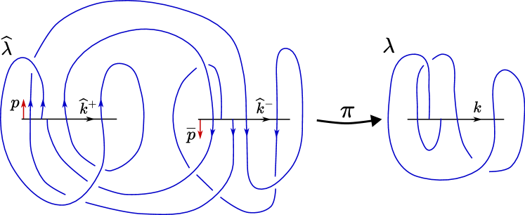
Figure 5: The figure depicts the orientation covering of a minimal geodesic lamination $\lambda$. The blue arcs represent homotopy classes of geodesic segments joining the relevant transversals; train tracks carrying $\widehat{\lambda}$ (or $\lambda$) can be obtained by collapsing $\widehat{k}^{\pm}$ (or $k$) to points.

Remark 7.6.

As in §7.1, the results in this subsection have analogues when $\lambda$ is not dynamically minimal. As before, one would choose a finite system of transversals and integrate the equivariant measure from their union to achieve an affine interval exchange transformation. We omit the details for tedium.

7.3 Relationship to affine laminations

For convenience choose a hyperbolic structure $X$ on a surface $S$ and a connected geodesic lamination $\lambda\subset X$. Let $\mathcal{N}$ be a snug train track neighborhood of $\lambda$. Let $\chi:\pi_{1}\mathcal{N}\rightarrow\mathbb{R}_{+}$ be a homomorphism and $\widetilde{\mathcal{N}}$ be a covering space of $\mathcal{N}$ for which $\pi_{1}\widetilde{\mathcal{N}}<\ker\chi$. Let $\widetilde{\lambda}\subset\widetilde{\mathcal{N}}$ be the pre-image under the covering map of $\lambda$.

Following Hatcher and Oertel [HO92], an affine lamination is a $\chi$-equivariant transverse measure supported on $\widetilde{\lambda}$. That is, a homotopy invariant transverse measure $\widetilde{\nu}$ satisfying

$$\chi(\gamma)\gamma.\widetilde{\nu}=\widetilde{\nu}$$ (21)

for all $\gamma\in\pi_{1}\mathcal{N}$ acting by deck transformations. Equivalently, for every transverse arc $k\subset\widetilde{\mathcal{N}}$ and every $\gamma\in\pi_{1}\mathcal{N}$, we have

$$\widetilde{\nu}(\gamma.k)=\chi(\gamma)\widetilde{\nu}(k),$$

where $\widetilde{\nu}(k)=\int~{}d\widetilde{\nu}_{k}$.

As always, there is a flat line bundle $E_{\chi}\to\mathcal{N}$ with holonomy $\chi$ defined as

$$E_{\chi}=\widetilde{\mathcal{N}}\times\mathbb{R}/\chi.$$

The constants in $\mathbb{R}$ give flat sections of $\widetilde{\mathcal{N}}\times\mathbb{R}$, i.e. sections $\widetilde{w}$ such that

$$\chi(\gamma)^{-1}\gamma.\widetilde{w}=\widetilde{w}.$$

Then

$$\widetilde{\nu}\otimes\widetilde{w}$$

is invariant under $\pi_{1}\mathcal{N}$, and descends to a well-defined object on the bundle $E_{\chi}$.

There is a description of affine measure on a lamination which does not reference a covering space. Following the notation from §6.1, let

$$\mathcal{A}=\{\psi_{\alpha}:\zeta^{-1}(U_{\alpha})\to U_{\alpha}\times\mathbb{R}\}$$

be an atlas of vector bundle charts for a flat $\mathbb{R}$-bundle $E$ over $\lambda$. In each chart $U_{\alpha}$, let $\nu_{\alpha}$ be a transverse measure to $\psi_{\alpha}(\lambda\cap U_{\alpha})$ which is invariant under transverse homotopy in the chart, and $\omega_{\alpha}:U_{\alpha}\cap\lambda\rightarrow E|_{\lambda}$ a flat section in the chart.

An affine measure on $\lambda$ valued in $E$ is then specified by the choice of an object of the form $\nu_{\alpha}\otimes\omega_{\alpha}$ on each chart. These choices are of course required to be coherent on overlaps of charts:

$$(\nu_{\alpha}\otimes\omega_{\alpha})|_{U_{\alpha}\cap U_{\beta}}=(\nu_{\beta}\otimes\omega_{\beta})|_{U_{\alpha}\cap U_{\beta}}.$$

If $\mathcal{N}$ is a snug train track neighborhood of $\lambda$ with $q:\mathcal{N}\to\tau$ the quotient by collapsing the ties, then by using Proposition 6.12 and pullback by the map $q:\lambda\subset\mathcal{N}\to\tau$, we may pass between bundles over the traintrack neighborhood, $\mathcal{N}$, the lamination, $\lambda$, and the train track, $\tau$.

Remark 7.7.

The two notions of affine lamination outlined above are the same. That is, to each affine lamination in the sense of Hatcher–Oertel, there is an affine line bundle and an affine lamination described in local charts (and vice versa). The proof is an exercise in covering theory.

The purpose of discussing affine laminations is the following result that ties together some of the main objects of study in this paper.

Theorem 7.8.

For $\mu\in\mathcal{ML}(X)^{G}$, let $\mathcal{N}$ be a (train track) neighborhood of $\lambda=\operatorname{supp}\mu$. Then the product

$$\mu\otimes[s^{1}]=\nu\otimes\omega$$

is an affine lamination on $\lambda$. The relevant bundle is $R^{\rho}_{2}\to\lambda$, the ray bundle got as a two-fold quotient of $F^{\rho}_{2}$. Its flat sections are the slithering sections constructed in Section 6.2 producing the holonomy representation $|\chi|:\pi_{1}\tau\to\mathbb{R}_{>0}$.

Proof.

Lemma 5.4 shows that $\mu\otimes[s^{1}]$ satisfies the required homotopy invariance. To show that it may be represented as a product of a flat section and a measure satisfying (21) on $\widetilde{\mathcal{N}}$ is Theorem 7.1 and Theorem 6.15. ∎

To each geodesic lamination and Hitchin representation $\rho:\pi_{1}S\to\operatorname{SL}(3,\mathbb{R})$, we have a flat ray bundle $R_{2}^{\rho}(\lambda)=F_{r}^{\rho}(\lambda)/(\pm 1)$.

Definition 7.9.

For each Hitchin representation $\rho:\pi_{1}S\to\operatorname{SL}(3,\mathbb{R})$, define

$$\mathcal{ML}^{\rho}(S)=\{(R_{2}^{\rho}(\lambda),\nu\otimes\omega)\}$$

as the set of pairs where $\lambda\subset S\text{ is a geodesic lamination and }\nu\otimes\omega\text{ is a nonzero affine measure on }R_{2}^{\rho}(\lambda)$.

We consider this space with its natural weak-$*$ topology.

If $\eta:\pi_{1}S\to\operatorname{Aff}^{*}(3,\mathbb{R})$ has linear part $\rho$, and bending cocycle $\psi$ with support $\lambda$, then Theorem 5.1 gives us a unique $\mu\in\mathcal{ML}(X)^{G}$ with $\psi=\mu\otimes s^{1}$. Theorem 7.8 tells us that $\mu\otimes[s^{1}]$ is an affine measure $\nu\otimes\omega$ on $R_{2}^{\rho}(\lambda)$.

In other words, there is a map

$$\beta_{+}:\{\eta:\pi_{1}S\rightarrow\operatorname{Aff}^{*}(3,\mathbb{R})~{}\text{irreducible}\mid L(\eta)\in\operatorname{SL}(3,\mathbb{R}).\rho\}/\operatorname{Aff}^{*}(3,\mathbb{R})\to\mathcal{ML}^{\rho}(S)$$ (22)

recording the affine bending data from a $\operatorname{Aff}^{*}(3,\mathbb{R})$ conjugacy class of representation with linear part (conjugate to) $\rho$. The ‘$+$’ decoration on this map reflects the global choice of a component of $\partial\Xi_{\eta}$. There is a map $\beta_{-}$ defined analogously for the opposite component.

Remark 7.10.

The flat ray bundle $R^{\rho}_{2}(\lambda)$ contains enough data to reconstruct the flat line-bundle $F^{\rho}_{2}(\lambda)$. The fibers of $F_{2}$ covers $R_{2}$ two-to-one, and the holonomy of $F_{2}$ picks up a minus sign based on topological data which can be seen in a train track carrying $\lambda.$ Therefore no data is lost by considering only the ray bundle.

Remark 7.11.

The fact that the slithering connection has non-trivial holonomy in general around the boundary components of a snug train track neighborhood of $\lambda$ (see (17)) makes it difficult to define an affine structure on the (dual) dendrite which is a quotient of the leaf space of $\lambda$.

7.4 Continuity of $\beta_{+}$

To a train track $\theta$ with branches $b(\theta)$, the weight space $W(\theta)$ is the vector subspace of $\mathbb{R}^{b(\theta)}$ cut out by the switch conditions. That is, a given $\phi\in W(\theta)$ satisfies for all switches

$$\sum\phi(b_{i}^{in})=\sum\phi(b_{j}^{out}),$$

where $b_{1}^{in},...,b_{k}^{in}$ are the incoming and $b_{1}^{out},...,b_{\ell}^{out}$ are the outgoing half-branches of $\theta$ at that (oriented) switch [PH92, Thu22]. There is a non-negative cone $W_{\geq 0}(\theta)$ obtained by intersecting $W(\theta)$ with $\mathbb{R}_{\geq 0}^{b(\theta)}$. Given a measure $\mu$ with support contained in a lamination carried by $\theta$, denote by $\mu(b)$ the integral of the constant function $1$ over a transversal to $b$. This function $w_{\mu}:b\mapsto\mu(b)$ is the non-negative weight system of $\mu$ on $\theta$.

The following lemma follows from (21) and the definitions.

Lemma 7.12.

An affine lamination with holonomy $\chi$, thought of as a transverse measure $\widetilde{\nu}$ on $\widetilde{\lambda}$, gives a weight system $w=w_{\nu}:b(\widetilde{\tau})\rightarrow\mathbb{R}$ satisfying

$$w(\gamma.b)=\chi(\gamma)w(b)\text{ for all $\gamma\in\pi_{1}\tau$.}$$

Remark 7.13.

By cutting $\tau$ along a finite collection of points (called stops), one can record these data as a weight system on a train track $\tau$ with stops and holonomy; see [HO92].

Suppose $\mu_{n}\in\mathcal{ML}(X)^{G}$ have support $\lambda_{n}^{\prime}$ and converge weak-$*$ to $\mu$ with support $\lambda^{\prime}$. Choose maximal completions $\lambda_{n}$ of $\lambda_{n}^{\prime}$. Passing to a subsequence, we assume that $\lambda_{n}$ converge in the Hausdorff topology to a geodesic lamination $\lambda$ that, necessarily, is maximal and contains $\lambda^{\prime}$. Let $\mathcal{N}$ be a snug train track neighborhood of $\lambda$ collapsing to $\tau$. Note that $\lambda_{n}$ is carried snugly by $\tau$ for large enough $n$.

According to Theorem 7.8 and Lemma 7.12, for each $n$, there are corresponding affine measures $\nu_{n}\otimes\omega_{n}$ and holonomy representations

$$|\chi_{n}|:\pi_{1}\tau\to\mathbb{R}_{>0}$$

and $|\chi_{n}|$-equivariant weight systems $w_{n}=w_{\nu_{n}}$. We also have the corresponding holonomy and weight system, $\chi$ and $w=w_{\nu}$, for $\nu$.

The following theorem states that equivariant transverse measures map continuously to affine measured laminations with the weak-$*$ topology.

Proposition 7.14.

For all $b\in b(\widetilde{\tau})$, the weight systems $w_{n}(b)\to w(b)$, as $n\to\infty$.

The proof relies on a continuity property of the slithering map indicated in the following Proposition. The techniques of Section 5 of [BD17] apply readily to give the proof, which we omit.

Lemma 7.15.

Suppose $\lambda_{n}$ are complete geodesic laminations converging in the Hausdorff topology to $\lambda$. Let $k$ be a transversal to $\lambda$, and lift the situation to the universal cover of $S$ so that $\widetilde{k}$ meets $\widetilde{\lambda}_{n}$ transversely for all $n$ large enough.

Let $\ell^{0}_{n}$ and $\ell^{1}_{n}$ be the first and last leaves of $\widetilde{k}\cap\widetilde{\lambda}_{n}$, ordered by $\widetilde{k}$. For each $n$, let $\Sigma_{n}\in\operatorname{SL}(d,\mathbb{R})$ be the slithering map defined by $\widetilde{\lambda}_{n}$ from $\ell^{0}_{n}$ to $\ell^{1}_{n}$. Define analogously $\ell^{0}$, $\ell^{1}$, and $\Sigma$ for $\lambda$.

Then $\Sigma_{n}\to\Sigma\in\operatorname{SL}(d,\mathbb{R})$.

Proof of Proposition.

7.14 Let $k$ be a transversal to some branch $b$. Without loss of generality, assume that for all $n$, $\omega_{n}$ is such that its evaluation on the leftmost leaf of $\lambda_{n}$ over $b$ is equal to $s^{1}$ evaluated on the same leaf.

For each $n$, we have $[s^{1}]=f_{n}\omega_{n}$, where $f_{n}:\lambda_{n}\cap k\to\mathbb{R}_{>0}$ is continuous. Lemma 7.15 gives that $f_{n}$ converge in the following sense: if $x_{n}\in\lambda_{n}\cap k\to x\in\lambda\cap k$, then $f_{n}(x_{n})\to f(x)$. Thus we can extend $f$ continuously to a function $\tilde{f}:k\to\mathbb{R}_{>0}$, and then find continuous extensions $\tilde{f}_{n}:k\to\mathbb{R}_{>0}$ of $f_{n}$ so that

$$\|\tilde{f}_{n}-\tilde{f}\|_{\infty}\to 0,\text{ as }n\to\infty.$$

Using the triangle inequality, for any continuous $g:k\to\mathbb{R}$, we have

$$\left|\int gf_{n}~{}d\mu_{n}-\int gf~{}d\mu\right|\leq\left|\int g\tilde{f}_{n}~{}d\mu_{n}-\int g\tilde{f}~{}d\mu_{n}\right|+\left|\int g\tilde{f}~{}d\mu_{n}-\int g\tilde{f}~{}d\mu\right|.$$

The second term goes to zero by weak-$*$ convergence, while the first is bounded by

$$\|g\|_{\infty}\|\tilde{f}_{n}-\tilde{f}\|_{\infty}\mu_{n}(k).$$

Since $\mu_{n}(k)\to\mu(k)$, this term goes to zero as well, proving the Proposition. ∎

While $\mathcal{ML}(X)^{G}$ was constructed from a choice of norm and parameterization of the geodesic flow on $T^{1}S$, $\mathcal{ML}^{\rho}(S)$ does not reference any such choice.

Theorem 7.16.

The map $\beta_{+}$ defined in equation (22) is a homeomorphism that is homogeneous with respect to positive scale. Consequently, the quotient by positive scale $\mathcal{PML}^{\rho}(S)$ is a sphere of dimension $6g-7$.

Proof.

The proof of Theorem 5.1 gives that $\mathcal{ML}(X)^{G}$ is identified with irreducible coaffine representations with linear part $\rho$ up to conjugation. Proposition 7.14 proves continuity of the map $\mathcal{ML}(X)^{G}\to\mathcal{ML}^{\rho}(S)$.

To see that $\beta_{+}$ is injective, consider two distinct points $\mu$ and $\mu^{\prime}\in\mathcal{ML}(X)^{G}$. If their supports differ, then the bundle factor in $\beta_{+}(\mu)$ and $\beta_{+}(\mu^{\prime})$ differ. If they are supported on the same lamination, then the measures differ on some transversal, and therefore the measure factors in the codomain differ.

Integration on sufficiently small transversals distinguishes measures, so the weak-$*$ topology on $\mathcal{ML}^{\rho}(S)$ is Hausdorff.

By taking positive scalar classes, the map $\beta_{+}$ induces a continuous injection from a compact space to a Hausdorff space, hence is a homeomorphism to its image.

The inverse to $\beta_{+}$ is given by writing the measure $\nu\otimes\omega=\mu\otimes[s^{1}]$ and passing the ratio $\omega/[s^{1}]$ over the tensor. Then $\mu\in\mathcal{ML}(X)^{G}$, and applying Theorem 5.1 again completes the proof. ∎

8 Appendix

We review a motivating example due to Ungemach [Ung19], with some simplifications and extensions. This appendix is designed to be largely self-contained, apart from the content of Section 2.

The apparent paradox of these examples is that while one has bent a representation along an isolated leaf of a lamination which accumulates to a simple closed curve, the data of such a deformation cannot be captured as a transverse measure on a lamination: such a leaf is never in the support of a transverse measure.

Therefore, some more sophisticated technology must be developed to describe analytically the data of convex cocompact coaffine deformations in terms of bending data on laminations. This paper provides an answer to this question; equivariant (affine) measures are the necessary extension, see Sections 4.2 and 7.1.

Example 8.1.

Let $\rho\in\operatorname{Hit}_{3}$ be non-Fuchsian, and let $\Omega\subset\operatorname{\mathbb{R}\textrm{P}}^{2}=\mathbb{P}(\mathbb{R}^{4}/[e_{4}])$ be the domain which $\rho(\pi_{1}S)$ divides. Assume that there exist two disjoint non-homotopic simple closed curves $c_{1}$ and $c_{2}$ in $S$ so that $1$ is not an eigenvalue of $\rho(c_{1})$ or $\rho(c_{2})$. One may also choose $c_{1}=c_{2}$. Let $\Lambda_{j}(c_{i})$ be the $j^{\textrm{th}}$ eigenvalue of $c_{i}$, ordered by magnitude.

We may assume that $c_{i}$ is oriented so that $\Lambda_{2}(c_{i})>1$ for $i=1,2$. Choose a lamination $\lambda\subset S$ consisting of exactly three leaves:

$$\lambda=c_{1}\cup c_{2}\cup m$$

where $m$ is an isolated leaf which accumulates to both $c_{1}$ and $c_{2}$. Assume also that for both $c_{1}$ and $c_{2}$, $m$ is asymptotic to $c_{i}$ in the negative direction with respect to their orientations.

Let $\eta_{0}$ be the reducible coaffine representation with linear part $\rho$ which preserves the hyperplane $[\ker e^{4}]\subset\operatorname{\mathbb{R}\textrm{P}}^{3}$ and let

$$dev_{0}:\widetilde{S}\rightarrow\Omega\subset[\ker e^{4}]$$

be a developing map so that $dev_{0}(\lambda)$ is a union of projective segments. The complement in $\widetilde{S}$ of the lamination is a disjoint union of countably many connected components:

$$\sqcup_{i\in I}X_{i}=\widetilde{S}\setminus\widetilde{\lambda}.$$

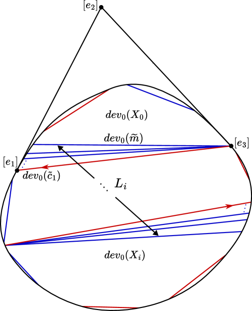
Figure 6: The domain $\Omega$ with the lifts of $c_{i}$ in red, and $m$ in blue. Two regions and the leaves between them are depicted.

Choose one such region $X_{0}$, and a point $\tilde{p}\in X_{0}$ projecting to $p\in S$, where $p$ is the basepoint implicit in $\pi_{1}S$. Assume (without loss of generality) that there is a lift $\tilde{m}\subset\partial X_{0}$. See Figure 6.

For each region $X_{i}$, let

$$L_{i}=\{\ell\subset\widetilde{\lambda}\mid\ell~{}\textrm{between}~{}X_{0}~{}\textrm{and}~{}X_{i}.\}$$

Let $M_{i}\subset L_{i}$ be those elements of $L_{i}$ which are translates of $\tilde{m}$. Because $m$ is not closed, each element of $M_{i}$ may be written as a $\eta_{0}$-translate of $\tilde{m}$ in a unique way, so that

$$M_{i}=\sqcup_{j\in J(i)}\eta_{0}(\gamma_{j}).\tilde{m}$$

for some countable index set $J(i)$.

From the discussion in Example 2.3, there exists a one-parameter subgroup $\{Z_{t}\}<\operatorname{TAff}^{*}(3,\mathbb{R})$ preserving $dev_{0}(\tilde{m})$ pointwise.

For each $t\in\mathbb{R}$ we define a developing map $dev_{t}$ which is equivariant with respect to a representation $\eta_{t}$. Define for each $i$ the translation

$$B^{t}_{i}=\sum_{j\in J(i)}\eta_{0}(\gamma_{j}).Z_{t}\in\operatorname{TAff}^{*}(3,\mathbb{R}).$$

Implicit in this definition is the claim that this sum converges. Asking the reader’s momentary trust, we then define $dev_{t}$ and $\eta_{t}$ as follows:

$$dev_{t}|_{X_{i}}=B^{t}_{i}.(dev_{0}|_{X_{i}})$$

and

$$\eta_{t}(\gamma)=B^{t}_{i(\gamma)}\eta_{0}(\gamma)\left(B^{t}_{i(\gamma)}\right)^{-1}$$

where $i(\gamma)\in I$ is the index of $\eta_{0}(\gamma).X_{0}$. This is essentially the standard construction of a developing map for a ‘bent’ representation in the sense of Johnson and Millson [JM87].

It is an exercise to check that $dev_{t}$ is $\eta_{t}$-equivariant. The geometry of the cone $\mathscr{C}\Omega$ discussed in Section 3.2 may be used to prove that $dev_{t}$ is a homeomorphism (one passes through the projection $[Q]$).

The interesting claim is that $B^{t}_{i}$ is well-defined, in particular that the countable sum defining it converges (absolutely). Briefly, it is sufficient to assume that $\tilde{m}$ and $\tilde{c}_{1}$ are asymptotic and to prove that the sum

$$\sum_{j=1}^{\infty}\eta_{0}(c_{1})^{n}.Z_{t}$$

converges absolutely. Choosing an ordered eigenbasis for $\eta_{0}(c_{1})$ reveals the equality

$$\sum_{j=1}^{\infty}\eta_{0}(c_{1})^{n}.Z_{t}=(b_{1}\sum_{j=1}^{\infty}\Lambda_{1}(c_{1})^{-n},b_{2}\sum_{j=1}^{\infty}\Lambda_{2}(c_{1})^{-n},0,0)$$

for some constants $b_{1},b_{2}\in\mathbb{R}$, where we have used the identification of $\operatorname{TAff}^{*}(3,\mathbb{R})$ with $\ker e_{4}$ to write a row vector rather than a matrix. Certainly, these geometric sums are absolutely convergent since $\Lambda_{1}(c_{1})>\Lambda_{2}(c_{1})>1$.

Note the direction onto which $m$ was chosen to accumulate onto $c_{1}$ and $c_{2}$ was crucial: otherwise these sums would exponentially diverge.

It is also true that the image of $dev_{t}$ is convex, though it is somewhat tedious to prove. Ungemach makes the necessary argument in Section 6 of [Ung19], or one may employ the techniques developed in Section 3.2. Thus, every lamination constructed in this way appears at the boundary of the convex hull for some convex cocompact coaffine representation. We omit the details of the proof for length.

M. D. Bobb, Max Planck Institute for Mathematics in the Sciences, Leipzig

E-mail address: mbobbmath@gmail.com

James Farre, Max Planck Institute for Mathematics in the Sciences, Leipzig

E-mail address: james.farre@mis.mpg.de

References

- [Aar97] Jon Aaronson, An introduction to infinite ergodic theory, Mathematical Surveys and Monographs, vol. 50, American Mathematical Society, Providence, RI, 1997. MR 1450400
- [ABB+07] Lars Andersson, Thierry Barbot, Riccardo Benedetti, Francesco Bonsante, William M. Goldman, François Labourie, Kevin P. Scannell, and Jean-Marc Schlenker, Notes on: “Lorentz spacetimes of constant curvature” [Geom. Dedicata 126 (2007), 3–45; mr2328921] by G. Mess, Geom. Dedicata 126 (2007), 47–70. MR 2328922
- [BD17] Francis Bonahon and Guillaume Dreyer, Hitchin characters and geodesic laminations, Acta Math. 218 (2017), no. 2, 201–295. MR 3733100
- [Ben04] Yves Benoist, Convexes divisibles. I, Algebraic groups and arithmetic, Tata Inst. Fund. Res., Mumbai, 2004, pp. 339–374. MR 2094116
- [Ben08] , A survey on divisible convex sets, Geometry, analysis and topology of discrete groups, Adv. Lect. Math. (ALM), vol. 6, Int. Press, Somerville, MA, 2008, pp. 1–18. MR 2464391
- [BF20] Thierry Barbot and François Fillastre, Quasi-Fuchsian co-Minkowski manifolds, In the tradition of Thurston—geometry and topology, Springer, Cham, [2020] ©2020, pp. 645–703. MR 4264589
- [Bon96] Francis Bonahon, Shearing hyperbolic surfaces, bending pleated surfaces and Thurston’s symplectic form, Ann. Fac. Sci. Toulouse Math. (6) 5 (1996), no. 2, 233–297. MR 1413855
- [Bon05] , Kleinian groups which are almost Fuchsian, J. Reine Angew. Math. 587 (2005), 1–15. MR 2186972
- [BPS19] Jairo Bochi, Rafael Potrie, and Andrés Sambarino, Anosov representations and dominated splittings, J. Eur. Math. Soc. (JEMS) 21 (2019), no. 11, 3343–3414. MR 4012341
- [BS85] Joan S. Birman and Caroline Series, Geodesics with bounded intersection number on surfaces are sparsely distributed, Topology 24 (1985), no. 2, 217–225. MR 793185
- [CB88] Andrew J. Casson and Steven A. Bleiler, Automorphisms of surfaces after Nielsen and Thurston, London Mathematical Society Student Texts, vol. 9, Cambridge University Press, Cambridge, 1988. MR 964685
- [CF23] Aaron Calderon and James Farre, Shear-shape cocycles for measured laminations and ergodic theory of the earthquake flow, to appear in Geom. Topol., Preprint arXiv:2102.13124, 2023.
- [CF24] , Continuity of the orthogeodesic foliation and ergodic theory of the earthquake flow, Preprint, arXiv:2401.12299, 2024.
- [CG93] Suhyoung Choi and William M. Goldman, Convex real projective structures on closed surfaces are closed, Proc. Amer. Math. Soc. 118 (1993), no. 2, 657–661. MR 1145415
- [CLM18] Suhyoung Choi, Gye-Seon Lee, and Ludovic Marquis, Deformations of convex real projective manifolds and orbifolds, Handbook of group actions. Vol. III, Adv. Lect. Math. (ALM), vol. 40, Int. Press, Somerville, MA, 2018, pp. 263–310. MR 3888622
- [Cob02] Milton Cobo, Piece-wise affine maps conjugate to interval exchanges, Ergodic Theory Dynam. Systems 22 (2002), no. 2, 375–407. MR 1898797
- [Dan13] Jeffrey Danciger, A geometric transition from hyperbolic to anti-de Sitter geometry, Geom. Topol. 17 (2013), no. 5, 3077–3134. MR 3190306
- [DGK23] Jeffrey Danciger, François Guéritaud, and Fanny Kassel, Convex cocompact actions in real projective geometry, Preprint, arXiv:1704.08711, 2023.
- [DS23] Farid Diaf and Andrea Seppi, The anti-de sitter proof of thurston’s earthquake theorem, Preprint, arXiv:2306.03631, 2023.
- [DS24] Bruno Dular and Jean-Marc Schlenker, Convex co-compact hyperbolic manifolds are determined by their pleating lamination, Preprint, arXiv:2403.10090, 2024.
- [EW11] Manfred Einsiedler and Thomas Ward, Ergodic theory with a view towards number theory, Graduate Texts in Mathematics, vol. 259, Springer-Verlag London, Ltd., London, 2011. MR 2723325
- [Far23] James Farre, Hamiltonian flows for pseudo-Anosov mapping classes, Comment. Math. Helv. 98 (2023), no. 1, 135–194. MR 4592854
- [GGKW17] François Guéritaud, Olivier Guichard, Fanny Kassel, and Anna Wienhard, Anosov representations and proper actions, Geom. Topol. 21 (2017), no. 1, 485–584. MR 3608719
- [Gha21] Selim Ghazouani, Teichmüller dynamics, dilation tori and piecewise affine circle homeomorphisms, Comm. Math. Phys. 383 (2021), no. 1, 201–222. MR 4236064
- [GLP09] C. Gutierrez, S. Lloyd, and B. Pires, Affine interval exchange transformations with flips and wandering intervals, Proc. Amer. Math. Soc. 137 (2009), no. 4, 1439–1445. MR 2465670
- [GS00] Gernot Greschonig and Klaus Schmidt, Ergodic decomposition of quasi-invariant probability measures, vol. 84/85, 2000, Dedicated to the memory of Anzelm Iwanik, pp. 495–514. MR 1784210
- [GW12] Olivier Guichard and Anna Wienhard, Anosov representations: domains of discontinuity and applications, Invent. Math. 190 (2012), no. 2, 357–438. MR 2981818
- [Hit92] N. J. Hitchin, Lie groups and Teichmüller space, Topology 31 (1992), no. 3, 449–473. MR 1174252
- [HO92] A. Hatcher and U. Oertel, Affine lamination spaces for surfaces, Pacific J. Math. 154 (1992), no. 1, 87–101. MR 1154734
- [JM87] Dennis Johnson and John J. Millson, Deformation spaces associated to compact hyperbolic manifolds, Discrete groups in geometry and analysis (New Haven, Conn., 1984), Progr. Math., vol. 67, Birkhäuser Boston, Boston, MA, 1987, pp. 48–106. MR 900823
- [Ker83] Steven P. Kerckhoff, The Nielsen realization problem, Ann. of Math. (2) 117 (1983), no. 2, 235–265. MR 690845
- [Ker85] , Simplicial systems for interval exchange maps and measured foliations, Ergodic Theory Dynam. Systems 5 (1985), no. 2, 257–271. MR 796753
- [Ker92] , Lines of minima in Teichmüller space, Duke Math. J. 65 (1992), no. 2, 187–213. MR 1150583
- [KH95] Anatole Katok and Boris Hasselblatt, Introduction to the modern theory of dynamical systems, Encyclopedia of Mathematics and its Applications, vol. 54, Cambridge University Press, Cambridge, 1995, With a supplementary chapter by Katok and Leonardo Mendoza. MR 1326374
- [KLP17] Michael Kapovich, Bernhard Leeb, and Joan Porti, Anosov subgroups: dynamical and geometric characterizations, European Journal of Mathematics 3 (2017), no. 4, 808–898.
- [Lab06] François Labourie, Anosov flows, surface groups and curves in projective space, Invent. Math. 165 (2006), no. 1, 51–114. MR 2221137
- [Mes07] Geoffrey Mess, Lorentz spacetimes of constant curvature, Geom. Dedicata 126 (2007), 3–45. MR 2328921
- [MMMZ23] Sara Maloni, Giuseppe Martone, Filippo Mazzoli, and Tengren Zhang, -pleated surfaces and their shear-bend coordinates, Preprint, arXiv:2305.11780, 2023.
- [MMY10] S. Marmi, P. Moussa, and J.-C. Yoccoz, Affine interval exchange maps with a wandering interval, Proc. Lond. Math. Soc. (3) 100 (2010), no. 3, 639–669. MR 2640286
- [NS22] Xin Nie and Andrea Seppi, Regular domains and surfaces of constant Gaussian curvature in 3-dimensional affine space, Anal. PDE 15 (2022), no. 3, 643–697. MR 4442837
- [PH92] R. C. Penner and J. L. Harer, Combinatorics of train tracks, Annals of Mathematics Studies, vol. 125, Princeton University Press, Princeton, NJ, 1992. MR 1144770
- [Roc70] R. Tyrrell Rockafellar, Convex analysis, Princeton Mathematical Series, vol. No. 28, Princeton University Press, Princeton, NJ, 1970. MR 274683
- [Smi17] ME Smith, On the unique ergodicity of quadratic differentials and the orientation double cover, arXiv preprint arXiv:1704.06303 (2017).
- [Ste51] Norman Steenrod, The Topology of Fibre Bundles, Princeton Mathematical Series, vol. vol. 14, Princeton University Press, Princeton, NJ, 1951. MR 39258
- [Thu82] William P. Thurston, Three-dimensional manifolds, Kleinian groups and hyperbolic geometry, Bull. Amer. Math. Soc. (N.S.) 6 (1982), no. 3, 357–381. MR 648524
- [Thu86] , Earthquakes in two-dimensional hyperbolic geometry, Low-dimensional topology and Kleinian groups (Coventry/Durham, 1984), London Math. Soc. Lecture Note Ser., vol. 112, Cambridge Univ. Press, Cambridge, 1986, pp. 91–112. MR 903860
- [Thu88] , On the geometry and dynamics of diffeomorphisms of surfaces, Bull. Amer. Math. Soc. (N.S.) 19 (1988), no. 2, 417–431. MR 956596
- [Thu98] , Minimal stretch maps between hyperbolic surfaces, Preprint, arXiv:math/9801039, 1998.
- [Thu22] , The geometry and topology of three-manifolds. Vol. IV, American Mathematical Society, Providence, RI, [2022] ©2022, Edited and with a preface by Steven P. Kerckhoff and a chapter by J. W. Milnor. MR 4554426
- [Ung19] Weston Ungemach, Deformations of Generalized Fuchsian Representations, ProQuest LLC, Ann Arbor, MI, 2019, Thesis (Ph.D.)–Stanford University. MR 4197617
- [Wan19] Jane Wang, The Geometry and Dynamics of Twisted QuadraticDifferentials, ProQuest LLC, Ann Arbor, MI, 2019, Thesis (Ph.D.)–Massachusetts Institute of Technology. MR 4051427
- [ZB04] Xiaodong Zhu and Francis Bonahon, The metric space of geodesic laminations on a surface. I, Geom. Topol. 8 (2004), 539–564. MR 2057773