[1,2]MauricioLima \Author[2]KatherineDeck \Author[2]Oliver R. A.Dunbar \Author[2]TapioSchneider
1]Ecole Polytechnique 2]Division of Geological and Planetary Sciences, California Institute of Technology
Mauricio Lima (mauriciodemouralima@gmail.com)
Toward Routing River Water in Land Surface Models with Recurrent Neural Networks
Abstract
Machine learning is playing an increasing role in hydrology, supplementing or replacing physics-based models. One notable example is the use of recurrent neural networks (RNNs) for forecasting streamflow given observed precipitation and geographic characteristics. Training of such a model over the continental United States has demonstrated that a single set of model parameters can be used across independent catchments, and that RNNs can outperform physics-based models. In this work, we take a next step and study the performance of RNNs for river routing in land surface models (LSMs). Instead of observed precipitation, the LSM-RNN uses instantaneous runoff calculated from physics-based models as an input. We train the model with data from river basins spanning the globe and test it in streamflow hindcasts. The model demonstrates skill at generalization across basins (predicting streamflow in unseen catchments) and across time (predicting streamflow during years not used in training). We compare the predictions from the LSM-RNN to an existing physics-based model calibrated with a similar dataset and find that the LSM-RNN outperforms the physics-based model. Our results give further evidence that RNNs are effective for global streamflow prediction from runoff inputs and motivate the development of complete routing models that can capture nested sub-basis connections.
The surface water cycle is a key component of the climate system (Oki and Kanae, 2006), and river routing of runoff from the land to the ocean is an important transport process simulated in Earth System Models (ESMs) (Li et al., 2015). Routing models provide a freshwater source to ocean models and have a range of additional applications, covering water resource management (He et al., 2017) to flood hazard assessments under climate change scenarios (Wobus et al., 2017).
Within an ESM, a river routing model must demonstrate generalizability across multiple temporal and spatial scales. In time, it should capture the seasonal cycle and the faster surface runoff response to precipitation events. In space, it must display generalizability across basins, one of the main challenges in modern hydrology (Sivapalan et al., 2003; Hrachowitz et al., 2013). River basins, the areas drained by individual rivers and its tributaries, tile the land surface into weakly connected domains, with water transport between basins given by the river streamflow. What we call basin generalizability, known in the hydrology community as regionalization, describes the skill of a model at using the learned characteristics of gauged basins (where streamflow is measured by streamgauges) to predict behavior in other, possibly ungauged, basins, generally in the same region at a sub-continental scale. Several approaches exist to tackle this problem (Prieto et al., 2019). What we call global basin generalizability refers to the same concept, but across all regions, and is also referred to as global-scale regionalization (Beck et al., 2016). In both cases, hydrological models that rely heavily on single-basin calibrations have greater difficulty generalizing due to overfitting to individual basins (Kratzert et al., 2024). Moreover, the vast majority of basins in many regions is ungauged; the generalization of models calibrated with basins from well-represented regions to those with a lack of gauges therefore is especially challenging (Feng et al., 2021).
A physics-based approach to river modeling can be implemented by adapting the shallow-water equations to a 1D setting under various approximations (Li et al., 2013). Two main processes are typically considered: hillslope routing and river channel routing (Mizukami et al., 2016). Hillslope routing describes how water moves across the landscape, considering factors such as topography, soil characteristics, and vegetation. It is the process that addresses the time lag between instantaneously generated runoff on land and the aggregation of runoff at a river outlet, forming the streamflow. This process is typically unresolved in river models used in ESMs and must be parameterized. In contrast, river channel routing describes how water moves from upstream channels to downstream outlets within the river network itself. Both the hillslope and river channel routing processes occur simultaneously within a basin. Physics-based representation of these processes present several advantages. First, the physical equations describing the flow naturally conserve water mass, which is crucial for systems simulated for long periods of time, as is the case in ESMs. Second, the interpretability of the model is straightforward since one knows exactly what physical laws are being used. Finally, physical laws have a long history of success in physical modeling; thus, these approaches are commonly employed in streamflow forecasting models across disciplines. For a more detailed overview of physics-based routing models, see Shaad (2018).
Recently, a class of recurrent deep learning models, referred to as Long-Short-Term-Memory (LSTM) models, have outperformed physics-based models on the rainfall-runoff problem (Kratzert et al., 2019b). In Kratzert et al. (2018), an LSTM was trained to model the entire land hydrology system for the continental United States. The model took observed precipitation as input (along with other dynamic inputs such as near-surface temperature, surface pressure, etc.) and then forecasted streamflow at the outlet of gauged catchments, implicitly modeling snowpack, soil storage, runoff, hillslope routing, and river channel routing. In Kratzert et al. (2019b), attributes such as topography, vegetation, and soil properties from different catchments were added to the model to improve its performance. The model did not explicitly account for routing between basins and treated each catchment independently. Nonetheless, the model showed good performance in regional calibrations, where a single set of parameters is learned using data from multiple catchments at once, employing large-sample hydrology data. Subsequently, predictions were made for the same basins that were used in training. Further studies also showed that these types of models were successful at basin generalization, forecasting basins not included in the training set (Kratzert et al., 2019a). This indicates that information in large-scale hydrological datasets is sufficient for generalization tasks, especially to the common ungauged basins (Nearing et al., 2021). In particular, it also suggests that these models are good candidates for representing processes that are not explicitly resolved in physical models (e.g., because they are below the model’s spatial resolution). Although machine learning (ML) models are not guaranteed to conserve mass a priori (or produce otherwise physical output, such as positive streamflow), constraints can be enforced by adapting the architecture of the network, for example, to be mass conserving (Hoedt et al., 2021).
0.1 Our contributions
Our goal in this work is to adapt the rainfall-runoff model (an LSTM) of Kratzert et al. (2019b) for use within a global LSM. To do so, we make several changes to the model architecture and training and validation procedures.
-
(i)
We use instantaneous runoff (both surface and sub-surface) as input, rather than precipitation, assuming that the runoff is provided by a separate land model. This is done to be able to keep track of where water is stored within the land surface. Keeping track of water fluxes (runoff, evaporation, transpiration) and storage (snow, soil, etc.) is crucial in LSMs for understanding interactions between key land surface components, such as soil, vegetation and snowpack, all of which interact with the atmosphere through energy and water fluxes (Bonan, 2019).
-
(ii)
We construct a globally consistent dataset to train and validate runoff-driven models. We incorporate runoff variables from reanalysis and use a globally unified system of basin characterizations, to ensure that our routing model can be integrated into an LSM in the future. This also requires addressing consistency between gauged catchments and geographical definitions of the nested sub-basins provided by our base dataset (Lehner et al., 2008). A similar idea was first introduced by the Caravan dataset (Kratzert et al., 2023), using precipitation instead of runoff.
-
(iii)
We evaluate the trained LSTM models on LSM-relevant tasks, including generalization across time and basins, using both continental and global training data. We demonstrate good performance of the model and interpret results at a granular level by breaking down skill over different geographical regions.
-
(iv)
We compare our generalization experiments with the physics-based LISFLOOD model (Van Der Knijff et al., 2010), which underlies the Global Flood Awareness System (GloFAS), run operationally by the European Copernicus program and at the European Centre for Medium-Range Weather Forecasts (ECMWF). To do so, we use the GloFAS discharge product provided as reanalysis (Harrigan et al., 2020). Results show the RNN approach displays superior performance, and we detail the steps taken to ensure this experiment was as fair as possible.
We note that the terms catchment and basin are often used interchangeably in the hydrology literature; however, in this paper we use “basin” (and sub-basin) for the units of topographical subdivision of the world into drainage areas and “catchment” for the drainage area of specific gauges.
The paper is structured as follows. Section 1 (Methods) presents the various components of our model, including data engineering and the training of the ML model. Section 2 (Results) presents our findings regarding temporal and basin generalization, a comparison to a physics-based model, and an investigation of model performance by basin attributes. Section 3 (Discussion and conclusion) summarizes the main results and outlines future directions.
1 Methods
1.1 Dataset
The first phase of this project consisted of constructing a consistent dataset that allows world-wide calibrations and simulations. Using global data for training is important as it increases the likelihood of generalization outside the training sample. In an ESM, river routing must be simulated across the entire globe, and not just across basins in the training set. To construct the dataset, we need both forcing data, which vary in time and space, as well as static attributes describing physical characteristics of each basin, which are assumed to only vary in space and which encode how runoff is routed within a basin. We additionally require streamflow data in each of these basins, which is the quantity our model is predicting. As explained in the introduction, we only target within-basin routing (hillslope routing and within-basin channels routing), and not main channel routing between nested sub-basins. This allows us to treat each basin as independent in training and simplifies the training task, at the expense of not making use of the information present in the river network structure. In practical terms, this implies that each catchment represented by a gauge in our data set must have a clear match to a basin.
1.1.1 Basins and static attributes
The HydroSHEDS dataset (Lehner et al., 2008) provides a vector-based division of the globe into basins (HydroBASINS, Lehner and Grill, 2013) viewable in levels (1 to 12) of resolution: as the levels grow, basins are subdivided into nested sub-basins, following the topography of the region. Moreover, each basin has static attributes derived from well-established global digital maps (HydroATLAS, Linke et al., 2019), which we use to construct the training data, as explained in Section 1.2. These static attributes are divided into seven sub-classes: Hydrology, Physiography, Climate, Land Cover & Use, Soils & Geology and Anthropogenic Influences. This offers a detailed description of basins that will be used to span the dimensional space in which our model operates. Static attributes are assumed to be constant over time and were chosen based both on previous studies (Kratzert et al., 2019b) and on our physical understanding of the problem. A table with all selected static attributes used in our models is shown in Appendix A. A particularly important static attribute is the area of the catchment, described in 1.1.3.
1.1.2 Dynamic inputs
Dynamic variables are the ones that change with time: sub-surface and surface runoff (mass attributes), temperature at 2-m height, surface pressure, and solar radiation over each basin. While in principle only mass attributes are required, additional variables were found to improve the accuracy of the model overall. Dynamic variables such as evaporation from rivers and re-infiltration are ignored. Water that is lost from river channels via these mechanisms is not explicitly tracked but can be implicitly present.
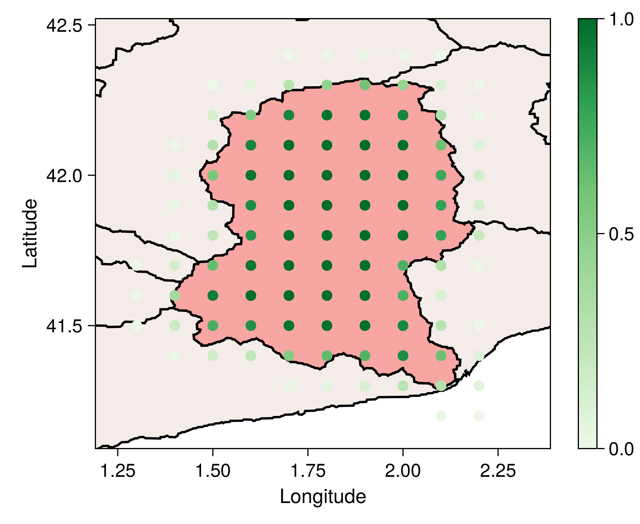
We derive a daily timeseries for each dynamic input for each basin using the grid-based reanalysis dataset provided by ERA5-Land (Muñoz-Sabater et al., 2021). Each point of the grid was attributed to the corresponding basin polygon in space using a simple ray-casting algorithm (Shimrat, 1962). To account for grid cells overlapping with basin boundaries, a Monte Carlo simulation was used to estimate how much of the cell area overlapped with the basin. We added noise to each grid point coordinate and computed the probability that a point is found inside the polygon. Figure 1a illustrates the process.
All dynamic variables are calculated daily. Sub-surface and surface runoff are extensive variables and are summed over the set of grid points inside each basin. The air temperature at 2-m height, the surface pressure, and the solar radiation are intensive variables and are averaged over the set of grid points inside each basin. Spatial averaging is applied to all variables within a basin, involving the division of the cumulative timeseries values within each basin by the corresponding number of grid points within that basin. We highlight that this process is feasible starting from any grid resolution, which makes the model adaptable to other datasets without the need for recalibration.
A final pre-processing step prior to training and network evaluation is to normalise all input variables, following Kratzert et al. (2022).
1.1.3 Streamflow
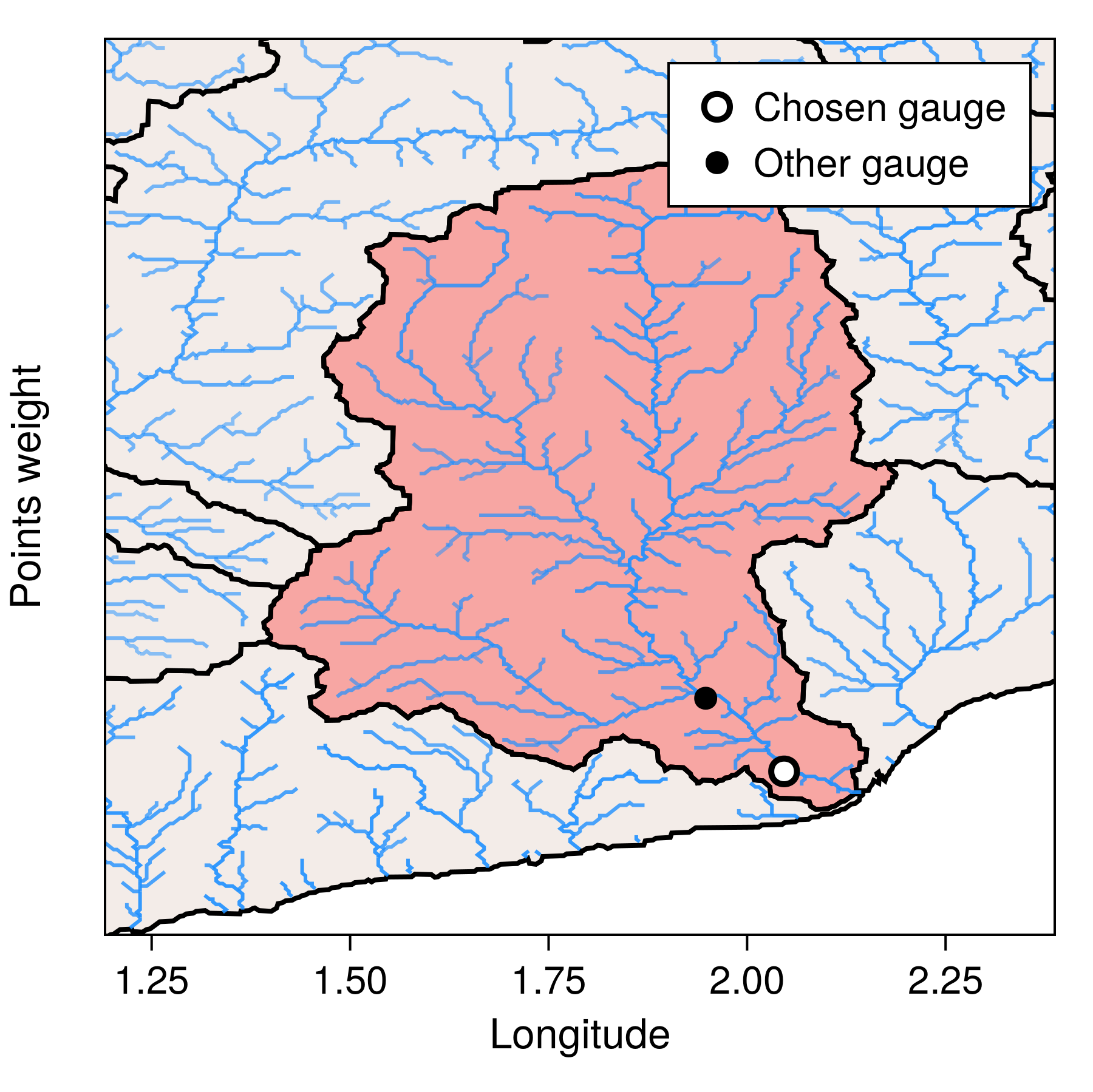
Measurements of streamflow as a function of time were obtained from the Global Runoff Data Centre (GRDC, 2023). To associate the discharge records from the river gauges, identified by latitude and longitude, with their corresponding basins, we employed the ray-casting algorithm to determine which polygon (basin vector) encloses each gauge. We found that in many cases, the gauge catchment area defined by GRDC and the basin area for the corresponding basin in HydroSHEDS were not in agreement. This can occur for two main reasons:
-
•
When a single gauge catchment area contains several small sub-basins, the catchment is much larger than the basin containing the gauge, which is probably a sub-basin dependent on upstream basins inside the catchment.
-
•
When a basin has smaller, secondary rivers with associated gauge catchment areas within it, the basin is much bigger than the gauge catchment within it, which probably corresponds to a sub-basin.
To reduce errors arising from assigning gauge catchment areas to the incorrect basin, we used a filter allowing not more than a 20% difference between the catchment and basin area. This value was chosen as a balance between a small threshold (favoring gauges closer to the outlet of the basin, hence more representative of the outflow of the basin) and a large threshold (favoring more matching examples, hence more data for calibration). Ultimately, this filter has the role of choosing only basins with good spatial agreement with their gauge catchment. Moreover, only gauges with more than 1 year of consecutive data were considered in the training phase. This procedure was inspired by Sutanudjaja et al. (2018). We highlight that not all basins have data in the test phase, which means that some basins can be used for training but not for testing. The result of this process is shown in Figure 1b.
The streamflow measurements provided by GRDC are in terms of the local time zone where the gauge is located. To match with ERA5-Land reanalysis, we interpolated these timeseries to UTC. As the GRDC timeseries have daily increments, this shift assumes a constant streamflow during the day, which is a coarse approximation. Furthermore, we take the gauge catchment area defined by GRDC (and not the basin area defined by HydroSHEDS) to use as static attribute for the gauge linked to a basin for model training. This variable is crucial for the model because it enables it to adjust the input runoff, normalized to the basin area, according to the size of the drainage area, in order to predict streamflow. All other static and dynamic inputs are estimated using the corresponding basin defined in HydroSHEDS.
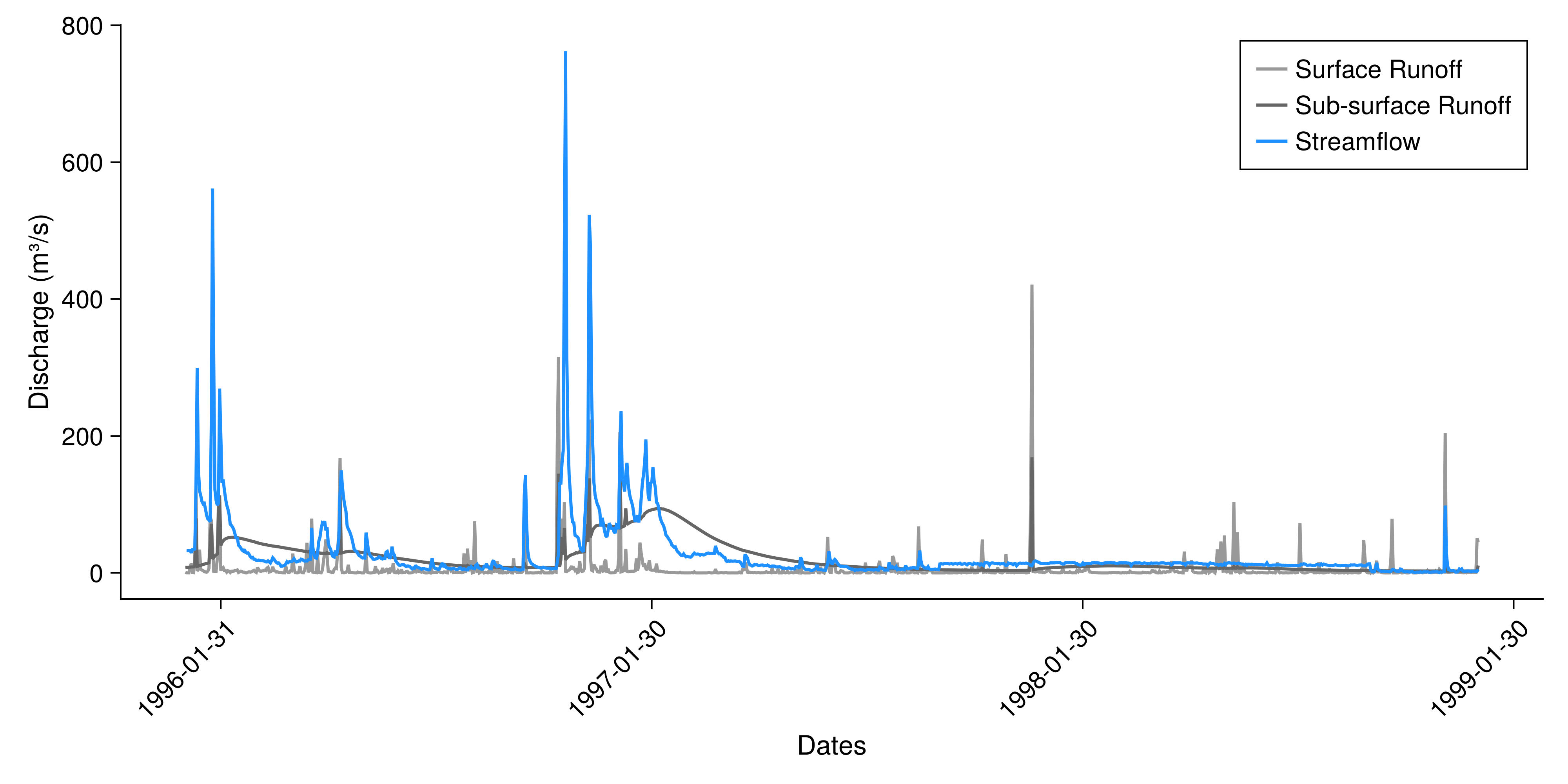
The resulting runoff and streamflow timeseries on the basin in Figures 1a and 1b is shown in Figure 2.
1.1.4 Dataset summary
The process was applied for all 9 continental areas and for 3 of the 12 levels available in HydroSHEDS (levels 5, 6, and 7). These levels were chosen based on their size (median values of 17,472 km2, 5,318 km, and 1,537 km2, respectively), which is relevant for typical resolutions of climate models. Table 1 summarizes the data. The study covered the time span from 1990 to 2019, with certain gauges exhibiting gaps in discharge data. No gap filling technique was applied, and only original values were retained.
| Level | US | Global |
| \tophlineLevel 05 | 55 | 224 |
| Level 06 | 150 | 443 |
| Level 07 | 193 | 660 |
| Combined levels | 398 | 1327 |
| \bottomhline |
1.2 LSTM model
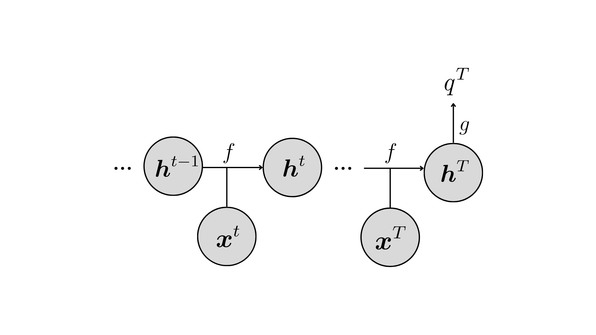
Recurrent neural networks are a subset of neural networks that contain recurrent connections and were designed to handle sequential data (Rumelhart et al., 1986; Goodfellow et al., 2016). RNNs are particularly effective when the predictor requires a (possibly long) time history data to make accurate forecasts. This is relevant to our use case, as the key variables (surface and subsurface runoff) are provided as a daily timeseries for each basin, but streamflow may depend on the time history of runoff because of physical storage and transport processes. Given an element in a sequence indexed by discrete time () and a set of learnable parameters , a hidden state in a typical RNN is completely described by the recurrent relation
| (1) |
where represent some flexible parametrized model, and this equation is subject to an initial condition . Here, is the vector concatenating the vector of dynamic variables and the vector of static attributes: ). At the final time , the corresponding output (daily streamflow in \unitm^3 s^-1) depends on the hidden state through
| (2) |
where is a function that is composed of a linear transformations and a dropout layer used to prevent overfitting (Srivastava et al., 2014). A schematic of the network is shown in Figure 3.
LSTMs (Long Short-Term Memory; Hochreiter and Schmidhuber (1997)) are a type of RNN with a specific general structure of the function . A detailed implementation of the LSTM network adapted for rainfall-runoff modeling can be found in Kratzert et al. (2018) and Kratzert et al. (2019b), on which our work is based. The design of the network avoids the vanishing gradient problem that plagues the training procedures for vanilla RNNs, so that optimization of the weights of an LSTM is far more effective. As an RNN, it also allows for the state at previous steps to affect the output at the current step.
Without additional constraints, there is no guarantee that the LSTM model conserves water mass (aside from indirectly, by matching observed streamflow given runoff as input). An important consideration for LSMs/ESMs is how to adapt this model in order to conserve mass, possibly accounting for processes like evaporation from rivers and re-infiltration of water into the soil. Possible approaches include changing the loss function or adapting the neural network design to be mass conserving (Hoedt et al., 2021); we leave such adaptations for future work. Specific details about the hyper-parameters used by our model can be found in Appendix B. More details can also be found in our code (Lima, 2024).
1.3 Metrics
To assess the performance of the model, we use the Nash-Sutcliffe efficiency (NSE, Nash and Sutcliffe, 1970), which, for a given outlet, can be written as
| (3) |
where and are the predicted and observed streamflow at the the basin outlet for time and is the averaged observed streamflow over all times in the period . In this expression, 1 is a perfect score (), and it gets worse (lower NSE) as the fraction of the mean squared error () normalized by the variance of the streamflow () increases. This normalization implies the NSE to lie in . Note that if a model is predicting only the mean flow at the outlet (i.e., ), we would have an NSE of 0. We will use this value as reference to evaluate good performances (NSE > 0) vs. bad performances (NSE < 0), as suggested in Knoben et al. (2019). The loss function optimized in the training of our models is an adaptation of the NSE. The adaptation and its motivation are explained in Kratzert et al. (2019b).
Another commonly used metric in hydrology is the Kling–Gupta efficiency (KGE, Gupta et al., 2009), which, for a given basin, can be written as
| (4) |
In the equation, is the linear correlation coefficient between simulated and observed timeseries; is the variability ratio, given by the ratio between the standard deviation in simulations and the standard deviation in observations ; is the bias ratio, given by the ratio between the mean in simulations and the mean in observations . This score represents an explicit decomposition of the normalized mean squared error into the three components , , and . The score likewise lies in , with 1 being a perfect score. We can define a reference value based on the KGE for a model predicting only the mean flow. In this case, we would have no correlation (), no variability ratio (), but a perfect bias ratio (), which gives a reference KGE of . We will use this reference value as a parameter to evaluate a good performance (KGE > ) vs. a bad performance (KGE < ).
As both scores are unbounded along the negative axis, outliers can lead to large negative values. Therefore, we use the median score (rather than the mean) over the entire ensemble of basins to quantify the results. In discussion of only well-performing basins (outperforming the meanflow reference), it is still useful to use the mean; we denote this metric as "MeanNSE>0" for the NSE and "Mean" for the KGE. Better models will have this mean closer to 1. We also define the fraction of poor-performing basins (worse than the meanflow reference) in the test set. We denote this metric as "%NSE<0" for the NSE and "%" for the KGE. Better models will have this fraction closer to zero. As both metrics are normalized, we can compare river discharges from basins with different sizes and regimes in different climates.
2 Results
We present a series of experiments carried out to quantify the performance of the model. We compare the behavior of a model driven with precipitation to that of one driven with runoff, and we compare the behavior of a model trained and tested in the USA with one trained and tested globally. To assess generalizability across basins and times, we experiment with different training/testing/validation splits. The model’s training time varied with the datasets and the longest run took 8h with one V100 GPU. Furthermore, we compare the performance of the model against the physics-based model LISFLOOD (Van Der Knijff et al., 2010), provided by the ECMWF reanalysis data as GloFAS-ERA5 (Harrigan et al., 2020), which uses similar input and calibration data. The hindcasts generated by both models are presented under various conditions, including those where both models produce poor hindcasts, those where the hindcasts are close to the median score, and those where each model demonstrates good performance. Finally, we analyze the performance by continent and other attributes. An analysis by HydroSHEDS levels is provided in Appendix C.
All models shown in this section are based on the basic LSTM architecture. An analysis of mass conservation for our LSTM can be found in Appendix D.
2.1 From precipitation in the USA to runoff worldwide
This series of experiments investigates the performance of LSTMs trained and validated using basins in the USA only and LSTMs trained and validated on global data. The USA was chosen as reference for being a well characterized region in terms of data availability and because it allows for a more direct comparison to previous results (Kratzert et al., 2019a, b). Our goals were to determine how the performance of the model changes when the dynamic input changes (from precipitation to runoff driven from reanalysis), to determine how the model performance changes when trained with more varied data (from the USA to the global case), and to investigate how the model performs at the basin and temporal generalization tasks.
2.1.1 Temporal generalization
To address these questions, we begin with a temporal training/validation split. The dataset was divided into three different timeseries for all basins: from 01/10/1999 to 30/09/2009 for training, from 01/10/2009 to 30/09/2019 for validation, and from 01/10/1989 to 30/09/1999 for testing. We compared the model trained on the USA with runoff input with the model trained on the USA with precipitation input. We also compared the performance of the model trained on the USA with runoff input with the model trained using the global data set with runoff input.
Figure 4 shows the results of the models trained in this time-split configuration (solid lines). Shown is the cumulative density function (CDF) of the NSE scores, truncated to , for the 5 different models analyzed. Since a perfect model has an NSE score of 1, the best models have a CDF that remains nears zero at all values of the NSE except at 1. The median NSE corresponds to .
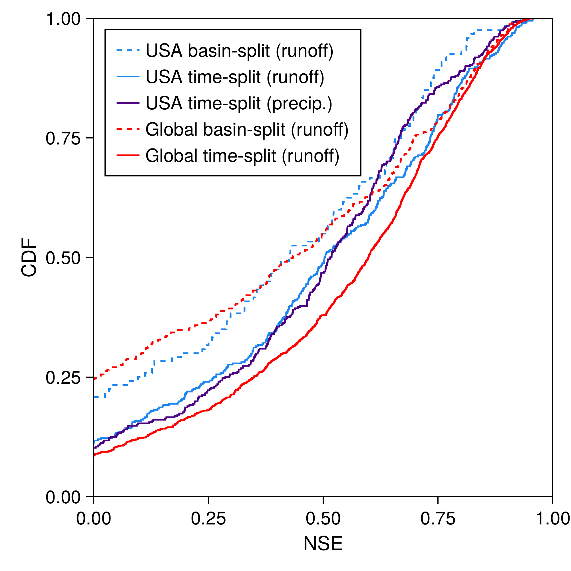
The results of the time-split experiment show that the model exhibits similar performance when we change the dynamic input data from precipitation to runoff. Quantitatively, we observe a median NSE of 0.50 for the runoff-driven model and a median NSE of 0.52 for the precipitation-driven model when both are trained on USA data. The model exhibits an increase in accuracy when trained with global data, yielding a median NSE of 0.60. This suggests that the model exhibits enhanced learning capabilities when trained on a more diverse dataset.
2.1.2 Basin generalization
We next investigate LSTMs trained on random subsets of all basins globally and test on a disjoint set of all basins globally. We divide our dataset of basins by choosing 70% for training (from 01/10/1999 to 30/09/2009) and validation (from 01/10/1989 to 30/09/1999) and 30% for testing (in the same time window as the training set). More precisely, from a total of 398 (USA) and 1327 (global) basins matched with gauges after the filters were applied, we use 278 (USA) and 928 (global) to train and validate and 120 (USA) and 399 (global) to test the model in this configuration. In this second set of experiments, we only compare models driven by runoff.
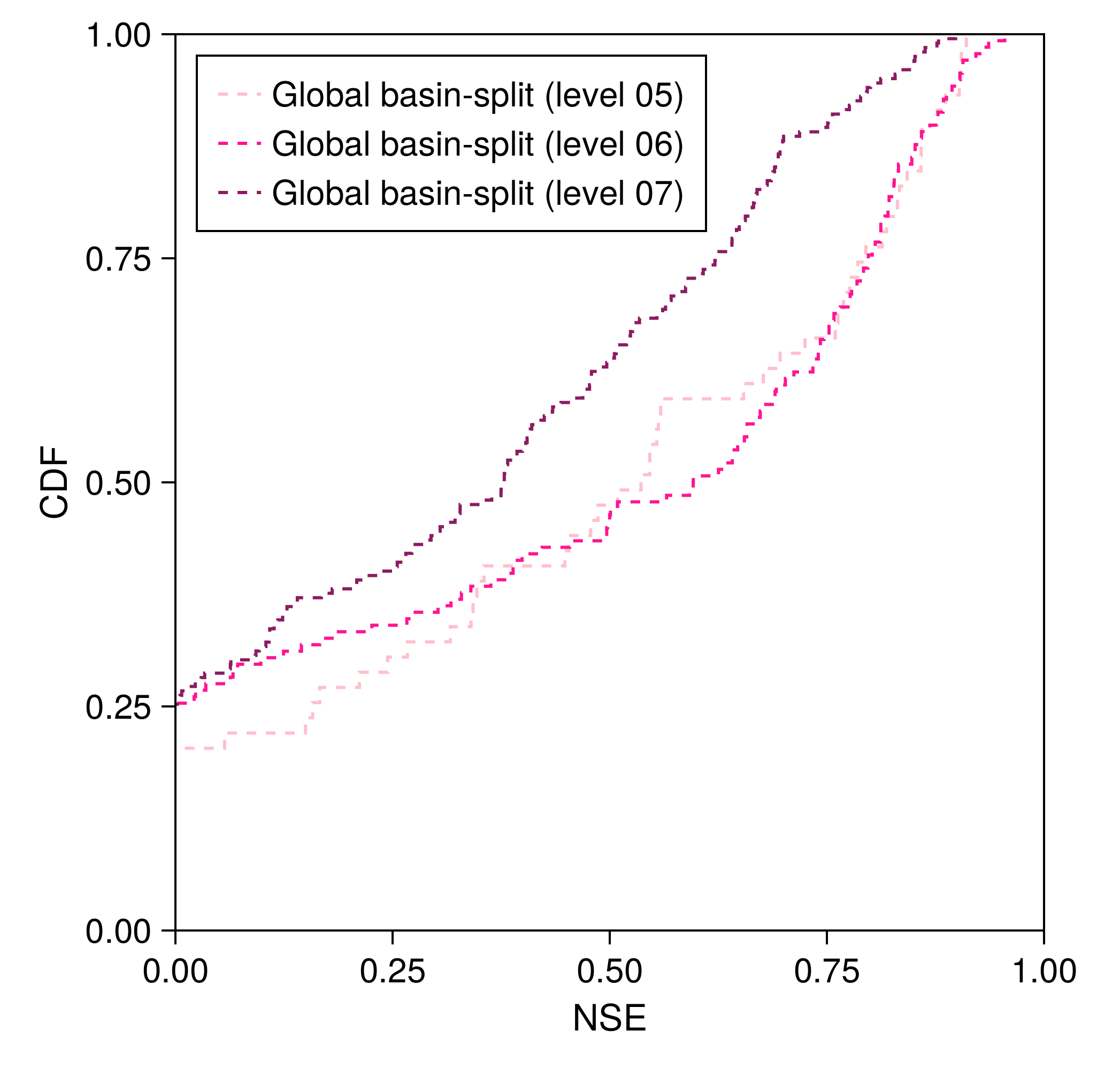
The results of the basin-split experiments are also shown in Figure 4 (dotted lines). The results demonstrate that the basin-split models perform more poorly compared with their counterparts trained with a time-split. This is expected as the unseen basins problem is a more challenging task. However, similar performances are observed in both the regionally calibrated (USA) and globally calibrated models: a median NSE of 0.43 is observed for both cases. In Appendix C, it is shown that the global basin-split model has a better performance for higher levels (05 and 06) in comparison to level 07, which means that the basin generalizability of the model does depend of the general size of the basins.
2.1.3 Summary of results
Table 2 highlights some important additional points. The time-split configuration trained on observed USA precipitation data has the smallest fraction of bad performances among the configurations trained and tested in the USA, suggesting that it suffers less from outliers and that there is room for improvement in runoff modeling. We also highlight that MeanNSE>0 is a good quantitative number to summarize the overall behavior of the curves in the CDF in Figure 4.
| Model | NSE | ||
|---|---|---|---|
| %NSE<0 | MeanNSE>0 | Median | |
| USA basin-split (runoff) | 20.83% | 0.51 | 0.43 |
| USA time-split (runoff) | 11.25% | 0.54 | 0.5 |
| USA time-split (precip.) | 10.23% | 0.53 | 0.52 |
| Globe basin-split (runoff) | 24.31% | 0.54 | 0.43 |
| Globe time-split (runoff) | 8.62% | 0.58 | 0.6 |
2.2 Comparison with physics-based model
In a second series of experiments, we compare the LSTM model with the LISFLOOD streamflow model (Van Der Knijff et al., 2010), provided by GloFAS-ERA5 (Harrigan et al., 2020). This choice was made mainly because, like LISFLOOD, our streamflow results are based on training a routing model with runoff from ERA5-Land as input. Moreover, the comparison between the LSTM and LISFLOOD was easy to do without additional calibrations, as the LISFLOOD streamflow predictions are provided with the reanalysis data.
That said, there are some important differences between our setting and that of GloFAS-ERA5: (i) LISFLOOD is a complete river routing model, whereas the LSTM models basins independently; (ii) the objective function for LISFLOOD is based on the KGE metric whereas the LSTM was trained to optimize NSE; and (iii) LISFLOOD is calibrated with a different global set of gauges. However, most of those gauges come from GRDC, as stated in Alfieri et al. (2020). When considering the validation time frame of the LISFLOOD model, it may coincide with the test period outlined in this paper, potentially simplifying the prediction task. However, we cannot be sure of this overlap. Hence, we presume the model to be configured more akin to a time-split configuration. To facilitate the comparison, we made an effort to provide a one-to-one relation between the LSTM/time-split training set and GloFAS-ERA5 by doing the following:
-
•
We consider only gauged basins that are independent of other basins, restricting the analysis to the set of basins used by our global model in the all-basins, time-split configuration;
-
•
We filter basins by allowing no more than a 20% difference between the catchment area of GRDC and the upstream area for the associated point from GloFAS, which we chose to be the grid point containing the gauge;
-
•
We filter basins by selecting only basins for which the corresponding grid cell in GloFAS lies entirely inside the basin polygon limits.
The process resulted in a total of 639 basins in the time-split and 190 basins in the basin-split configurations, which is about half the basins used in the global dataset. Using these basins, we evaluate the LSTMs in both time-split and basin-split configurations, after training with the previously described global data with no additional calibration. The LSTMs are evaluated against GloFAS-ERA5 for the corresponding time periods.
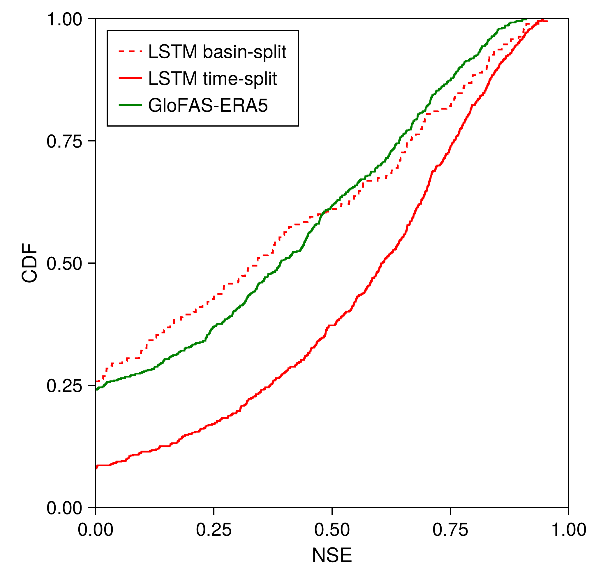
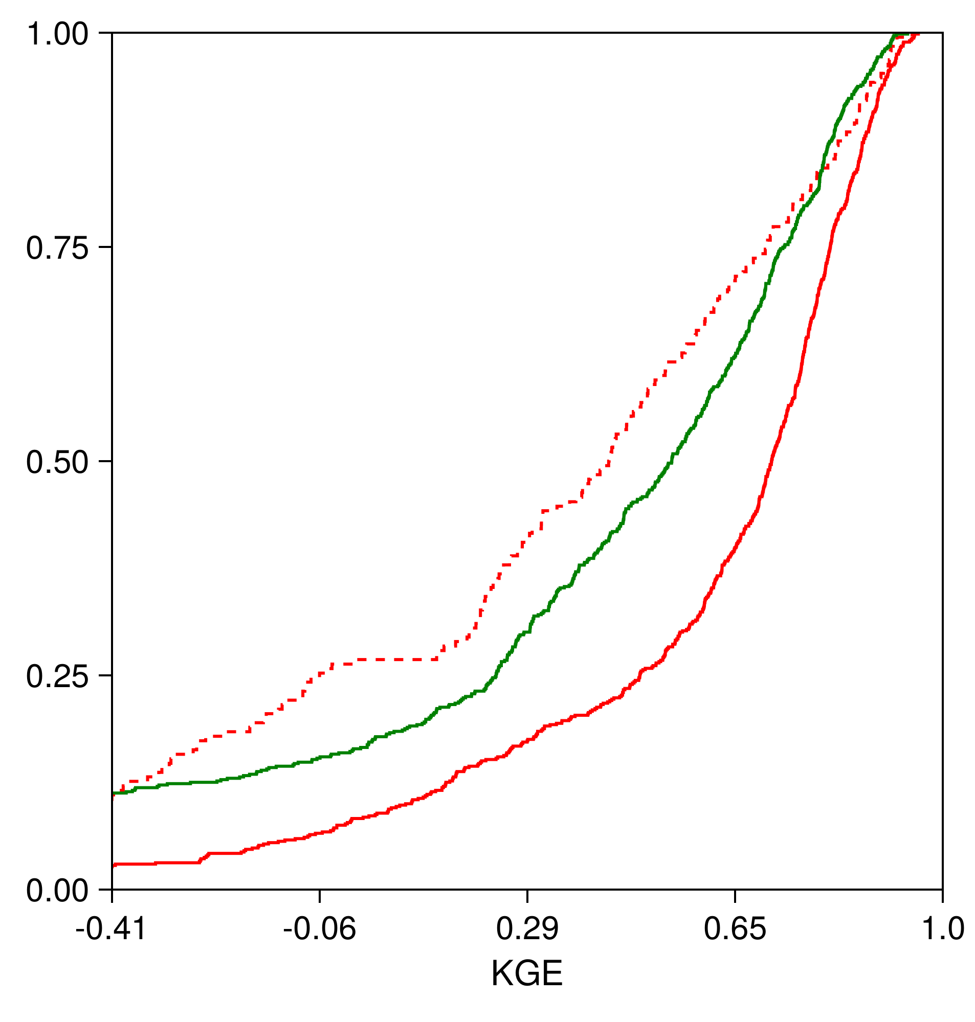
Figure 5 shows the comparison between the LSTM trained in the time-split and basin-split configurations and the physics-based benchmark. Figure 5a shows the CDF for the NSE score, which is the score that our model was designed to optimize. Figure 5b shows the CDF for the KGE score, which is the score optimized by GloFAS.
For the gauges we use, the LSTM in the time-split configuration shows an overall better accuracy compared with GloFAS, while the LSTM in the basin-split configuration displays a worse median accuracy in both metrics. For the NSE, the LSTM has a median score of 0.61 in time-split and 0.34 in basin-split configuration, whereas GloFAS displays a median score of 0.39. For the KGE, the LSTM has a median score of 0.71 in time-split and 0.43 in basin-split configuration, whereas GloFAS displays a median score of 0.54. In both cases, GloFAS (which, as we highlighted, is believed to be in a configuration closer to a time-split) is quantitatively closer to the LSTM basin-split configuration. This highlights the capabilities of the LSTM model, since the basin-split is a more difficult configuration. We show other metrics in Table 3.
| Model | NSE | KGE | |||||
|---|---|---|---|---|---|---|---|
| %NSE<0 | MeanNSE>0 | Median | % | Mean | Median | ||
| LSTM basin-split | 25.26% | 0.49 | 0.34 | 11.05% | 0.42 | 0.43 | |
| LSTM time-split | 7.98% | 0.59 | 0.61 | 2.66% | 0.62 | 0.71 | |
| GloFAS-ERA5 | 24.1% | 0.50 | 0.39 | 11.27% | 0.52 | 0.54 | |
The LSTM models perform better here compared with when evaluated on the data in section 2.1. This may suggest that the set of basins used to compare with the GloFAS benchmark contains gauges with more reliable measurements.
2.3 Simulations vs. Observed streamflow
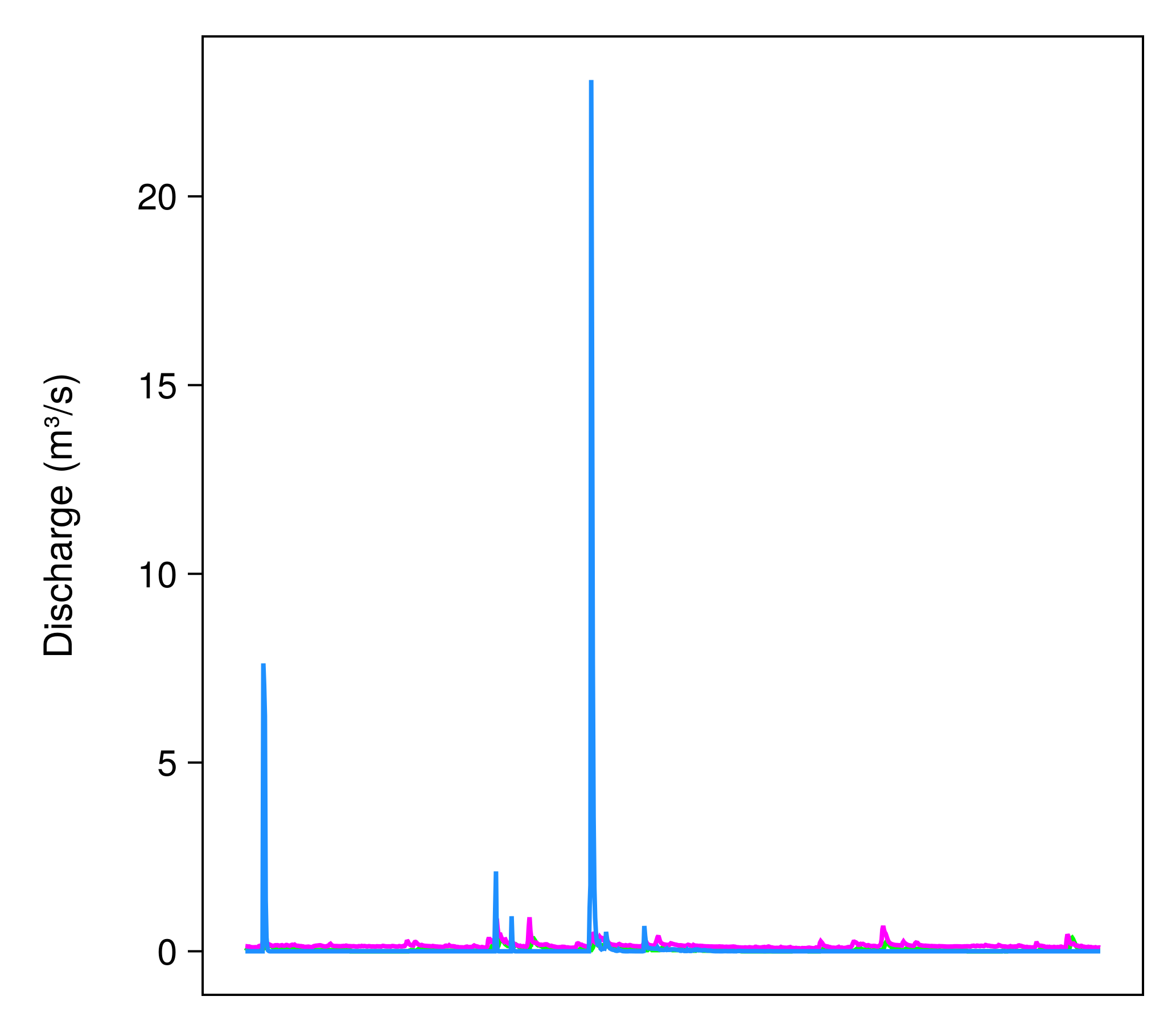
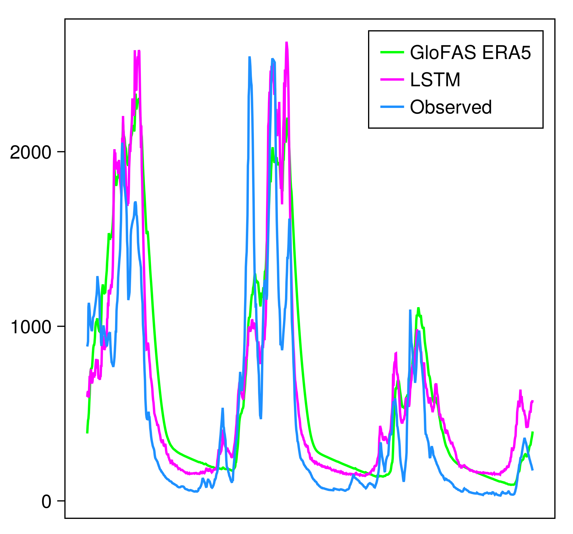
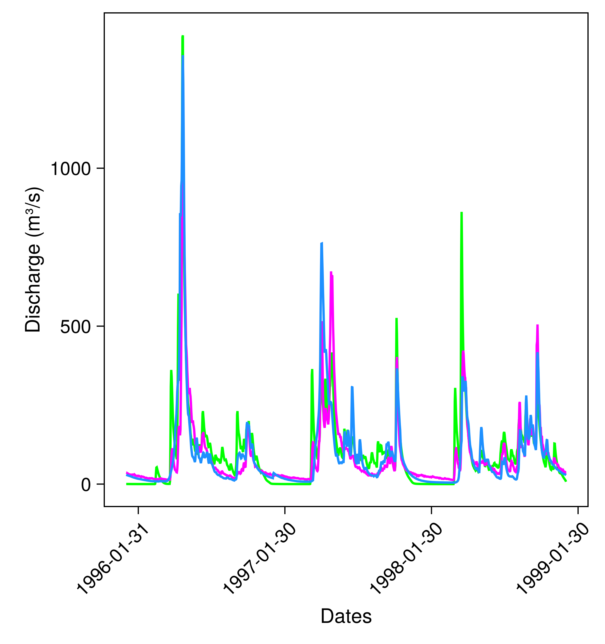
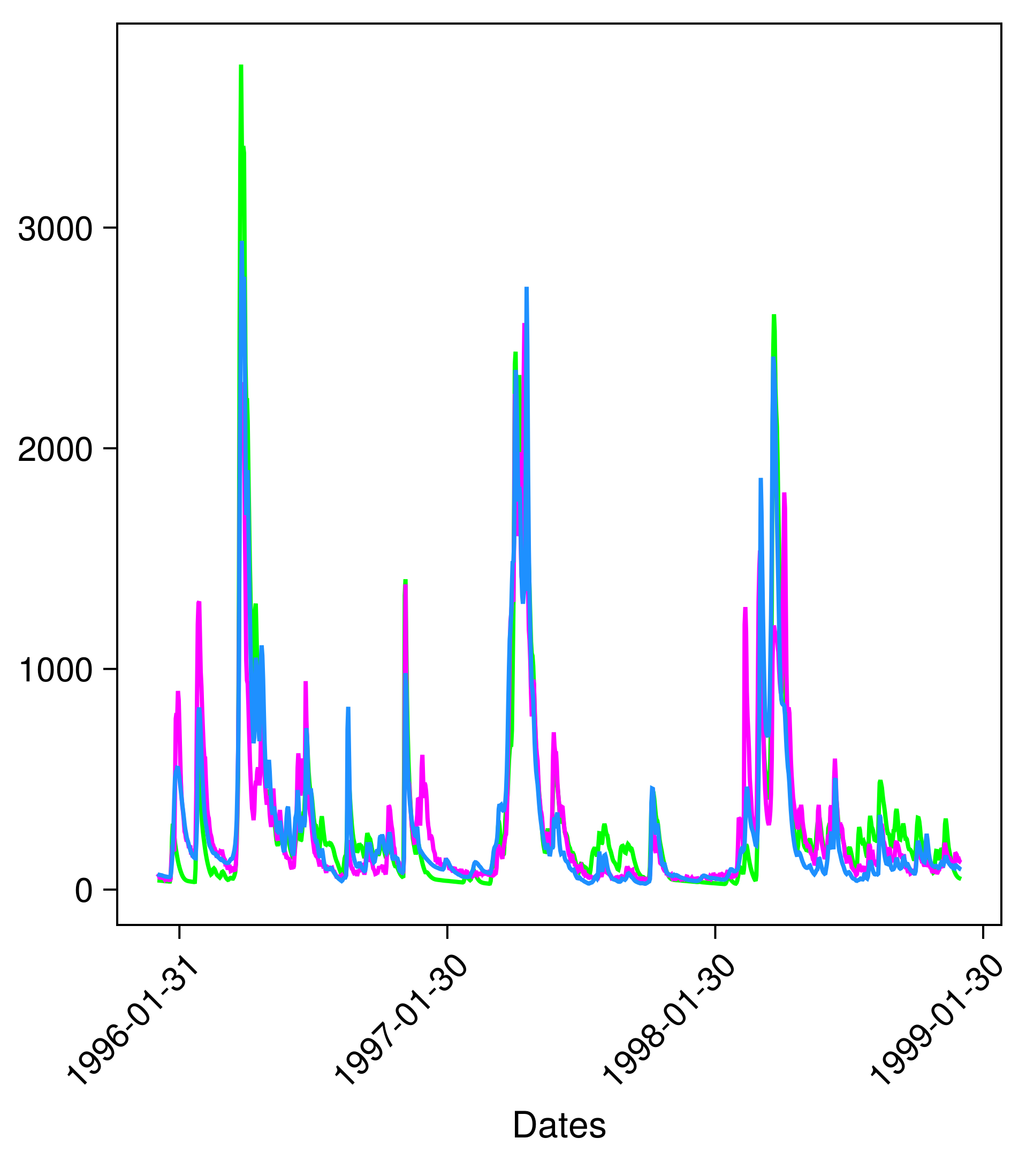
In this section, we present some simulated timeseries along with observations for various values of NSE and KGE to get a visual sense of performance. For four different basins, Figure 6 shows the predictions of the LSTM model in the global time-split configuration, the GloFAS-ERA5 reanalysis, and the observed streamflow at the corresponding GRDC gauge.
In the first example (Figure 6a), we have a poor performance in both NSE/KGE scores for both the LSTM model (/) and for GloFAS reanalysis (/). For both models, this is due to underprediction of a peak in the streamflow. This specific basin (1061638580 in HydroSHEDS level 06) is located in South Africa, and the corresponding gauge is located at the Seekoei River. It has a significantly lower streamflow than the other basins in the figure. (We come back to trends in the model performance with basin characteristics in the following section.) The next example (Figure 6b) lies around the median performance of our model: (/) for the LSTM model and (/) for GloFAS reanalysis. This basin (6050344660 in HydroSHEDS level 05) is located in Brazil, and the corresponding gauge is located at the Itacaiúnas River. The third plot (Figure 6c) shows an example where the LSTM model has a very good performance (/) and outperforms GloFAS slightly (/). This specific basin (7070250410 in HydroSHEDS level 07) is located in Canada, and the corresponding gauge is located at the North French River. The last plot (Figure 6d) shows a case where GloFAS (/) outperforms the LSTM model (/). This specific basin (7060363050 in HydroSHEDS level 06) is located at the border between Canada and the United States, and the corresponding gauge is located at the Saint John River.
2.4 Geographic patterns
Lastly, we investigate the performance of the LSTM model trained with global runoff data in the time-split configuration, for different basin characteristics and geographic properties.
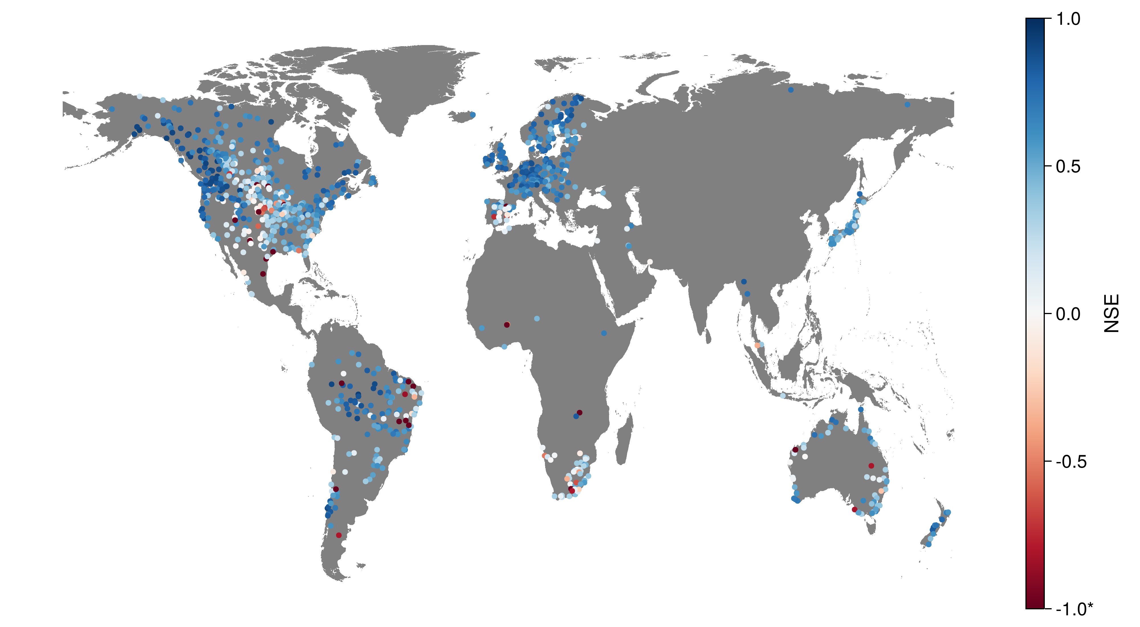
Table 4 shows statistics of NSE scores for each continental basin. We can see that regions that are under-represented in the data (such as Africa and Australasia) have worse scores, but that under-representation in terms of location is not enough to predict poor performance. In particular, the basins in Asia are well modeled from only 38 examples, and Siberia is well-modeled from only 2 examples. These results may be explained by the similarity of climate conditions between these regions and other well-represented regions. For example, conditions may be similar between Siberia and the Canadian Arctic.
| Continental basin | NSE | Number of basins | ||
|---|---|---|---|---|
| %NSE<0 | MeanNSE>0 | Median | ||
| Africa | 25.33% | 0.3 | 0.19 | 75 |
| Europe and Middle East | 4.32% | 0.67 | 0.71 | 301 |
| Siberia | 0.0% | 0.72 | 0.72 | 2 |
| Asia | 5.26% | 0.56 | 0.59 | 38 |
| Australasia | 9.41% | 0.49 | 0.47 | 85 |
| South America | 10.0% | 0.57 | 0.58 | 170 |
| North and Central America | 10.04% | 0.56 | 0.54 | 528 |
| Arctic (northern Canada) | 0.0% | 0.69 | 0.7 | 101 |
| Greenland | - | - | - | 0 |
The global distribution of NSE scores for the gauges in Table 4 can be seen in Figure 7. From the map, we see the contrast between data-rich regions (North America and Europe) and data-poorer regions (East Asia and central and northern Africa).
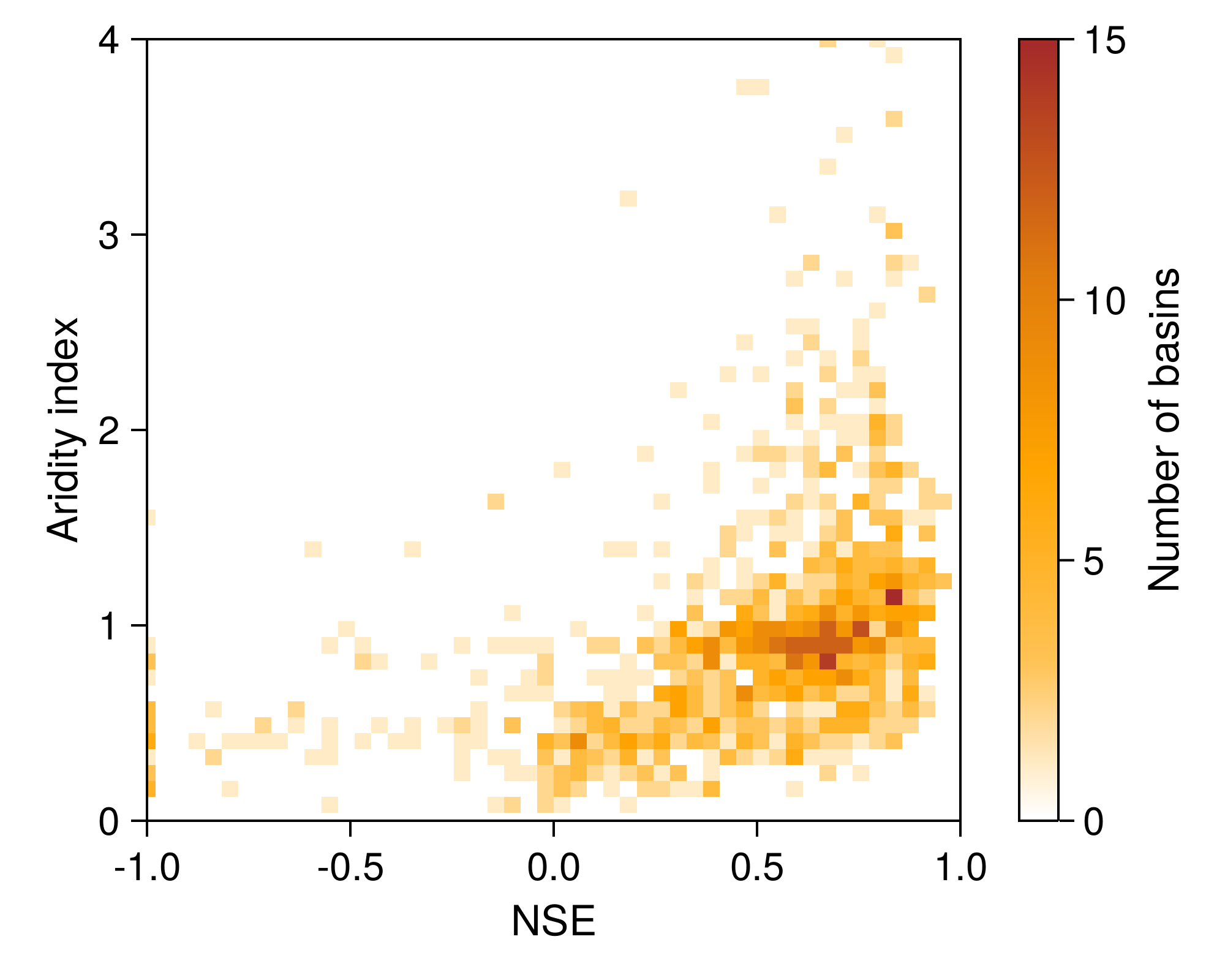
We also investigate the aridity index, which is provided in the HydroATLAS dataset (Linke et al., 2019) and has been found to be a strong predictor of the model’s performance. Figure 8 shows a trend toward poorer performance in drier regions (i.e., regions with lower aridity index), consistent with findings in Feng et al. (2020), but now on a global scale. (For context, the basin depicted in Figure 6a has an aridity index of 0.26.) This trend extends to other variables, such as mean runoff, for which the model also shows poorer performance in drier regions.
3 Discussion and conclusion
Long short-term memory models have been shown to be the state of the art for modeling streamflow in hydrological systems (Kratzert et al., 2019b), but most studies using these models have so far been restricted to specific regions, and they have focused on representing the entire land hydrological system as a single entity (Kratzert et al., 2019b; Koch and Schneider, 2022). However, for integration into the land surface models used in climate modeling, it is crucial for river models to demonstrate proficiency in generalizing across basins and temporal scales globally, using both surface and subsurface runoff data, rather than, for example, precipitation data. This necessity arises because traditional river models in land surface models merely route water, leaving the modeling of snow, soil, and vegetation hydrological processes to other model components. In this study, we have taken concrete steps toward developing an ML model that can substitute traditional river routing models within LSMs. We have successfully trained and validated an LSTM at the task of predicting streamflow from runoff worldwide.
We began our analysis by contrasting the results from an observed precipitation-driven model, which holistically represents land hydrology, with those of a modeled runoff-driven model. For the United States, we found that an LSTM trained only to route runoff performs comparably to one designed to simulate the entire land hydrology system (Kratzert et al., 2019b), even when trained on potentially less accurate and biased runoff data. A possible drawback of our approach is that it relies on modeled runoff from reanalysis as training data, which likely is less accurate than using precipitation data directly. Recently, other studies have used precipitation data on a global scale to simulate streamflow from LSTMs, being able to outperform the GloFAS model even when trained in a basin-split configuration, similar to the one made on this work (Nearing et al., 2024). However, it is not clear if this increase in performance is due to a change in the LSTM model, training data, or due to the forcing data used.
Our exploration into the model’s generalization capabilities revealed that a globally trained model, as opposed to one trained exclusively using data from the USA, achieved superior performance when both were fed runoff data in a time-split configuration. This improvement underscores the potential benefits of incorporating diverse global data. However, when evaluating models trained in the basin-split configuration, the performance gain was not as pronounced, highlighting the complex challenge of global basin generalization. This challenge is exacerbated by imbalances in global data availability and the wide range of possible climate conditions across the globe, which may not be well sampled in geographically localized training data (e.g., from the USA).
In comparison to the reanalysis data from the physics-based LISFLOOD model (GloFAS-ERA5), our LSTM model showed more accurate forecasts in a gauged scenario (time-split) but fell short in an ungauged scenario (basin-split). We argued that results from GloFAS-ERA5 are closer to a gauged (time-split configuration) scenario than an ungauged (basin-split) scenario. Thus, these findings suggest that our LSTM model holds promise for global basin generalization, despite the discrepancies between scenarios.
Additionally, our analysis revealed a correlation between the model’s performance and the aridity index, suggesting that drier regions pose unique challenges for the LSTM model. This could be due to the model’s difficulty in capturing short-term precipitation events that trigger streamflow peaks in these areas, as seen in Figure 6a (Feng et al., 2020). It also underperformed in regions likely underrepresented in the training data. Despite these challenges, the model’s time generalizability was consistent across different basin sizes, even if better basin generalizability was observed for bigger basins, as discussed in Appendix C. We highlight that the model doesn’t need to be re-calibrated for the evaluation of different basin levels.
In conclusion, our study presents a promising step toward using neural networks for water routing in the LSM component of climate models. The promising results motivate further research to refine these models for comprehensive river routing and integration into climate models. Future efforts will focus on designing training strategies to mitigate error propagation across connected basins and incorporating architectural adjustments to ensure mass conservation (e.g., (Hoedt et al., 2021)), potentially enhancing long-term simulation accuracy.
All data used to generate our training and test data are open source. The source code for the data engineering, the models, the extraction from the benchmark, and the visualizations can be found in https://github.com/maumlima/Rivers.
Appendix A List of static attributes used in the models
Table 5 lists the static attributes used in our models. \appendixtables\appendixfigures
| Variable Name | Description | Units |
| \tophlinepre_mm_syr | mean precipitation | \unitmm |
| ari_ix_sav | aridity index | \unit- |
| area | GRDC catchment’s area | \unitkm^2 |
| ele_mt_sav | mean elevation | \unitm |
| snw_pc_syr | snow percent cover | \unit- |
| slp_dg_sav | mean slope | \unit- |
| kar_pc_sse | karst percent cover | \unit- |
| cly_pc_sav | clay percent cover | \unit- |
| pet_mm_syr | mean potential evaporation | \unitmm |
| for_pc_sse | forest percent cover | \unit- |
| snd_pc_sav | sand percent cover | \unit- |
| slt_pc_sav | silt percent cover | \unit- |
| gwt_cm_sav | ground water table depth | \unitcm |
| run_mm_syr | land surface runoff | \unitm |
| soc_th_sav | organic carbon content | \unitt/ha |
| swc_pc_syr | soil water content | \unit- |
| sgr_dk_sav | stream gradient | \unitdm/km |
| cmi_ix_syr | climate moisture index | \unit- |
| \bottomhline |
Appendix B Hyper-parameters
Table 6 lists the most important hyper-parameters used in the model in the global time-split configuration. The learning rate started at and gradually decreased to during the 35 epochs of training.
| Hyper-parameter | Value |
|---|---|
| \tophlineHidden state | 256 |
| Droput rate | 0.4 |
| Length of input sequence | 270 |
| \bottomhline |
Appendix C NSE by HydroSHEDS level
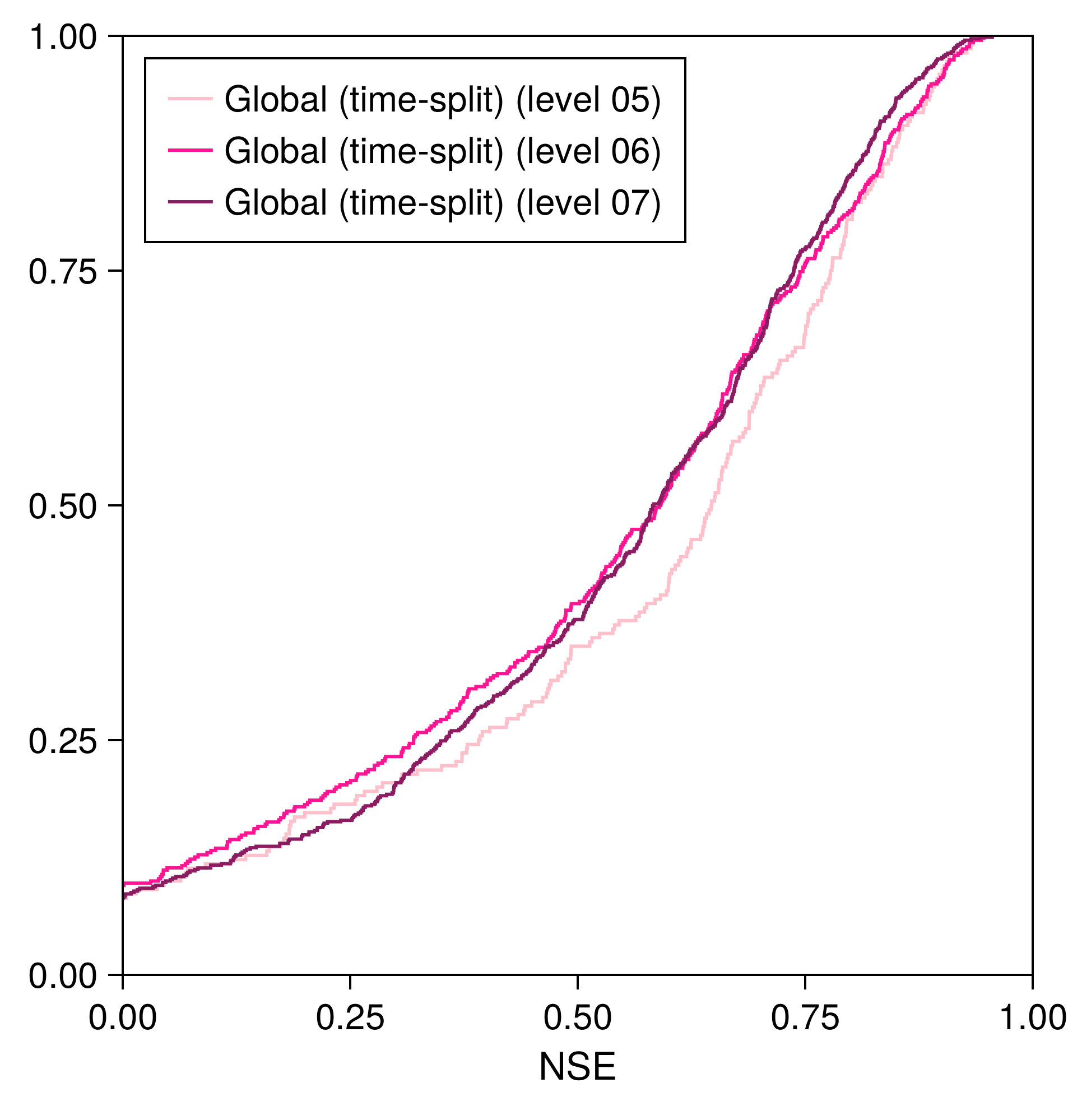
In this section, we show the the distribution of NSE scores for each of the three HydroSHEDS levels used in the training. The three levels differ in the typical size of basin areas. In Figure 9b, the consistency of the model is re-assuring because it shows that the model is able to adapt to different basin sizes under the same training set. In spite of that, Figure 9a shows that the model generalizes better to unseen basins for larger basins, as it has higher scores for levels 05 and 06 in comparison with level 07 - even if the latter is more represented in the training set. The LSTM in the basin-split configuration slightly outperformed GloFAS under the NSE metric when only evaluated in levels 05 and 06 – a median of 0.47 was observed against a median of 0.45. Even though, GloFAS was still better under the KGE metric – a median of 0.47 against 0.60.
Appendix D Mass balance
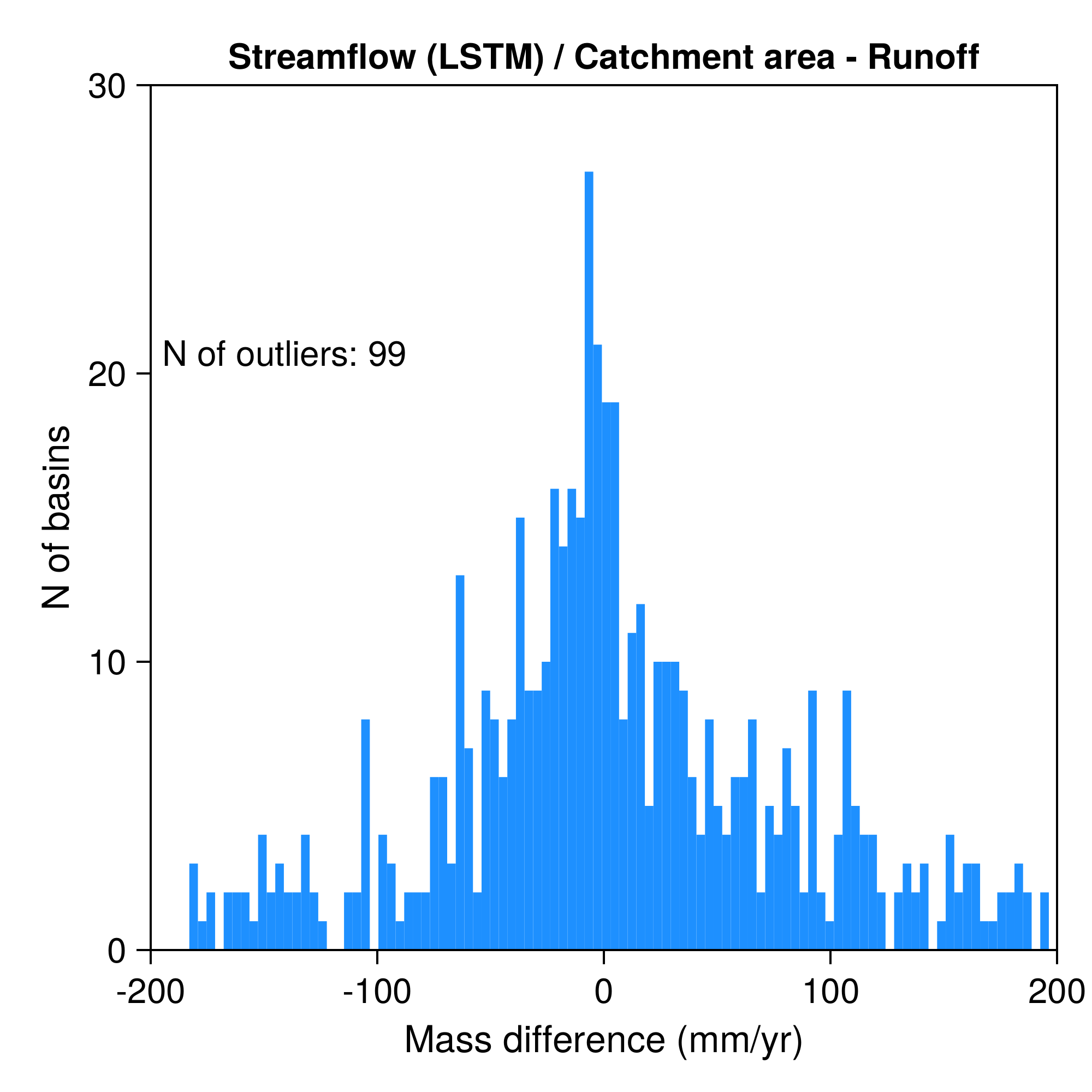
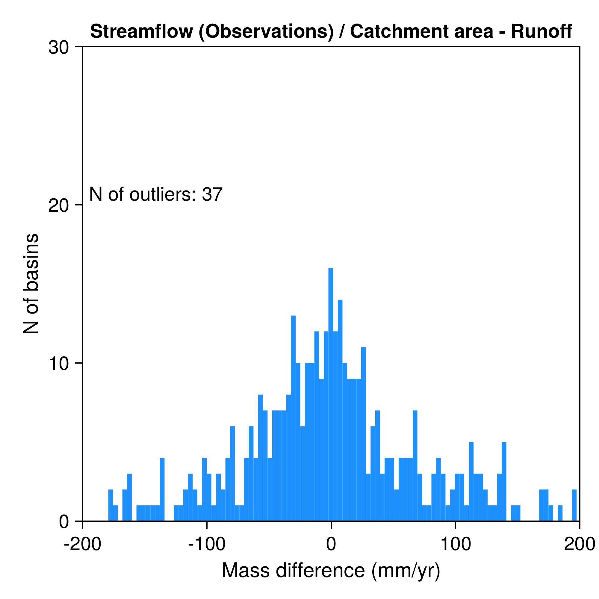
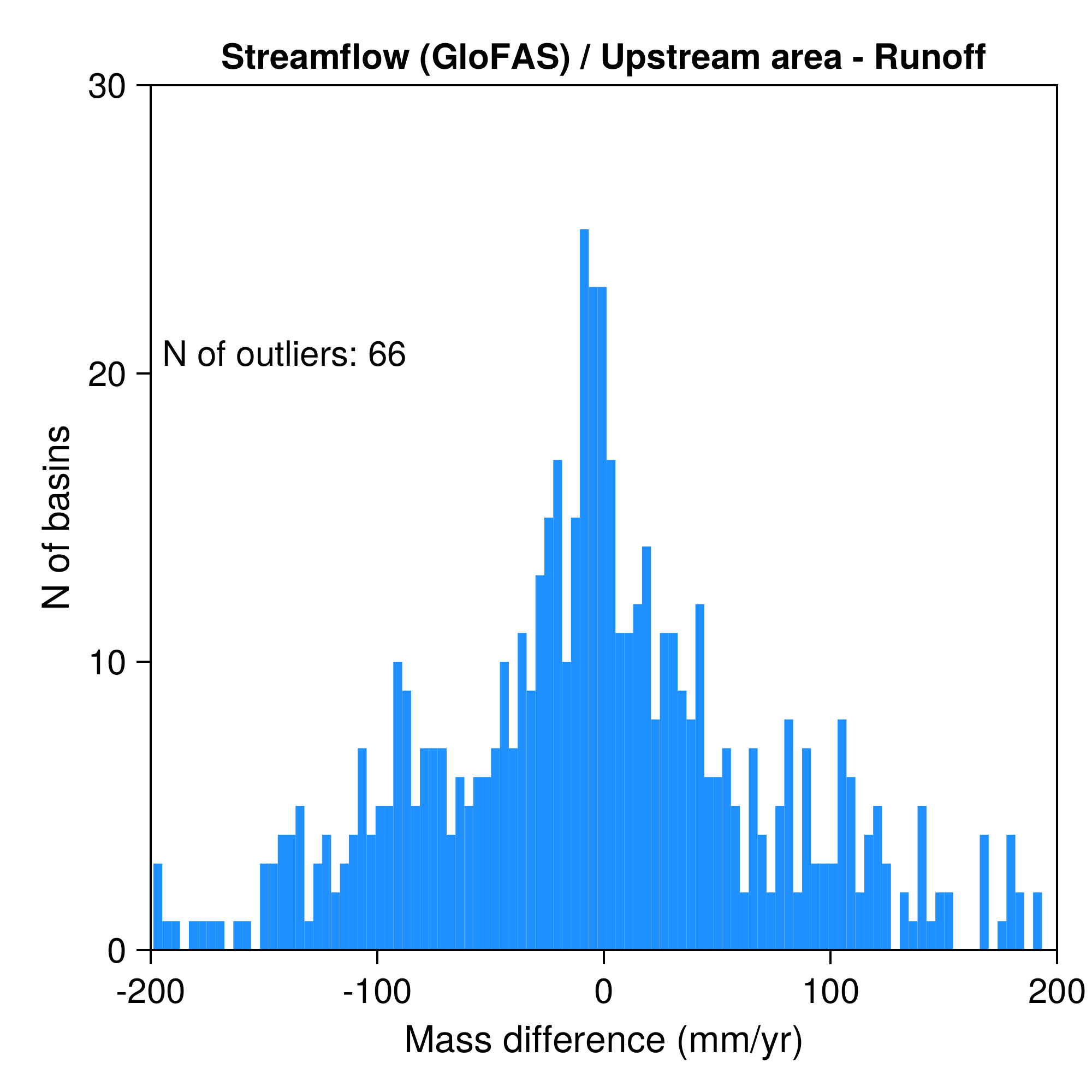
If there is no loss of water due to infiltration into deeper layers in the ground or evaporation into the atmosphere, the sum of runoff over the area of a catchment should match the discharge at the outlet when averaged over extended periods. We calculate the absolute difference between the outflow from each basin (normalized by its area) and the total runoff within the corresponding catchment over a 9-year time window. The results of this calculation are presented in Figure 10 for streamflow (in blue): forecasted by the LSTM (Figure 10a), recorded by observations from GRDC gauges (Figure 10b), and provided by the GloFAS reanalysis (Figure 10c). In each case, the number of outliers (“N of outliers”) represents the quantity of data points falling outside the boundaries of the graphs. These results indicate that the LSTM conserves mass at a level comparable to the observations and a physical model. While this is a positive result, it implies that additional processes like evaporation from rivers, re-infiltration of water into the ground, and human interference may need to be understood and modeled in order to achieve a closed water balance. One could expect to find a better mass conservation from the physics-based model, but it should be noted that GloFAS has parameters which control mass loss (to underground storage, for example) and the actual state of mass conservation can vary depending on the version of runoff data that was used in their calculations.
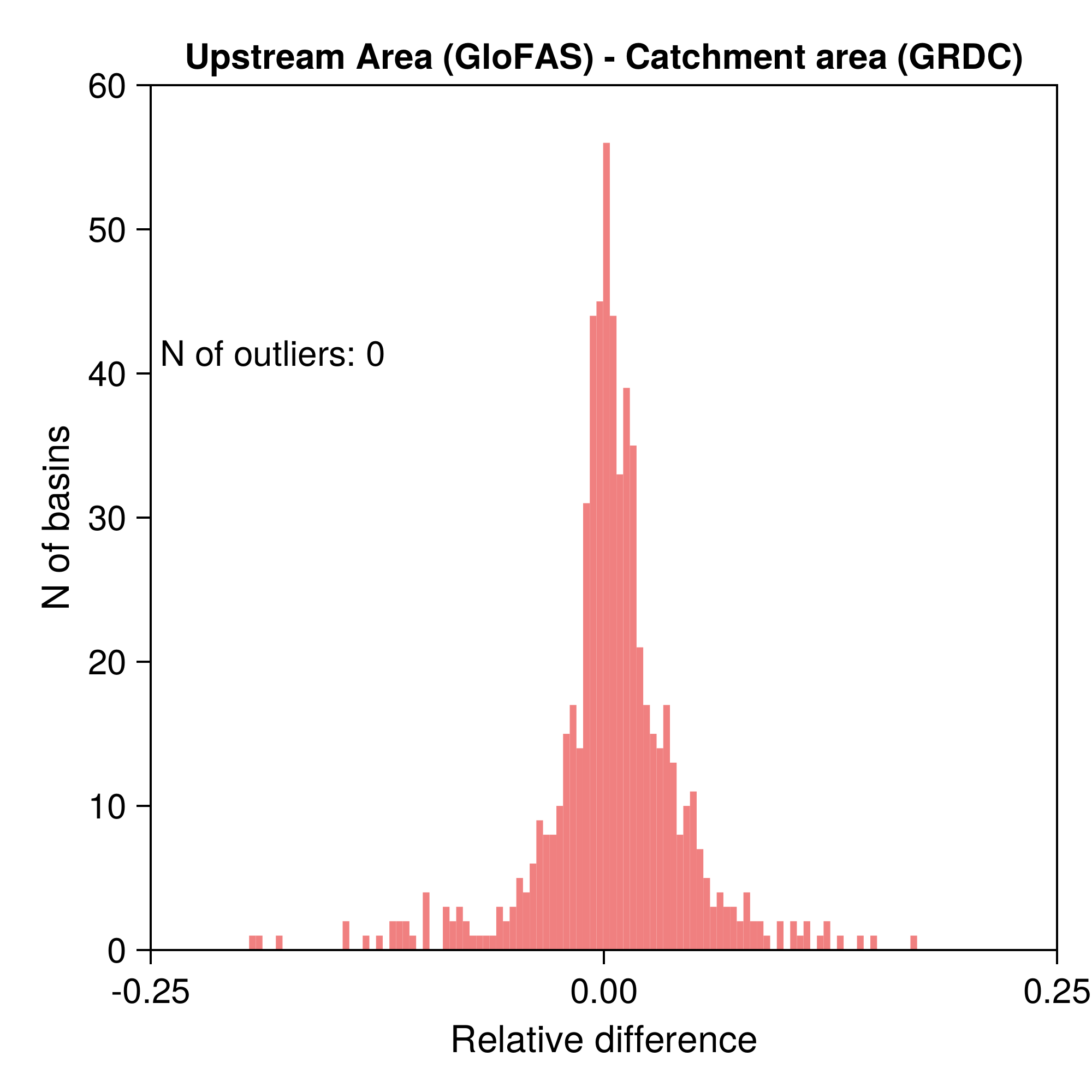
We also depict the relative difference between the definitions of upstream area and catchment area for each of these gauges (in pink). These relative differences are generally small. This implies that there is a good correspondence between the upstream areas used by GloFAS for the calculation of streamflow from runoff inputs and the area used in this study (provided by GRDC).
Acknowledgements.
This research was supported by the generosity of Eric and Wendy Schmidt by recommendation of the Schmidt Futures program. We thank Frederik Kratzert for a helpful early conversation, as well as the other maintainers of neuralhydrology, for the clear and helpful code. We also acknowledge Akshay Sridhar, who assisted with technical parts of the code and data handling, as well as insightful conversations. All numerical calculations and model training used for this manuscript were performed with the help of Caltech’s Resnick High Performance Computing Center.References
- Alfieri et al. (2020) Alfieri, L., Lorini, V., Hirpa, F. A., Harrigan, S., Zsótér, E., Prudhomme, C., and Salamon, P.: A global streamflow reanalysis for 1980–2018, Journal of Hydrology X, 6, 100 049, 10.1016/j.hydroa.2019.100049, 2020.
- Beck et al. (2016) Beck, H. E., Van Dijk, A. I. J. M., De Roo, A., Miralles, D. G., McVicar, T. R., Schellekens, J., and Bruijnzeel, L. A.: Global-scale regionalization of hydrologic model parameters, Water Resources Research, 52, 3599–3622, 10.1002/2015wr018247, 2016.
- Bonan (2019) Bonan, G.: Climate Change and Terrestrial Ecosystem Modeling, Cambridge Univ. Press, Cambridge, UK, 2019.
- Feng et al. (2020) Feng, D., Fang, K., and Shen, C.: Enhancing streamflow forecast and extracting insights using Long-Short term memory networks with data integration at continental scales, Water Resources Research, 56, 10.1029/2019wr026793, 2020.
- Feng et al. (2021) Feng, D., Lawson, K., and Shen, C.: Mitigating prediction error of deep learning streamflow models in large Data-Sparse regions with ensemble modeling and soft data, Geophysical Research Letters, 48, 10.1029/2021gl092999, 2021.
- Goodfellow et al. (2016) Goodfellow, I., Bengio, Y., and Courville, A.: Deep Learning, MIT Press, http://www.deeplearningbook.org, 2016.
- GRDC (2023) GRDC: Global Runoff Data Center, https://www.bafg.de/GRDC/EN/Home/homepage_node.html, accessed on July 7, 2023, 2023.
- Gupta et al. (2009) Gupta, H. V., Kling, H., Yılmaz, K. K., and Martínez, G.: Decomposition of the Mean Squared Error and NSE Performance Criteria: Implications for Improving Hydrological Modelling, Journal of Hydrology, 377, 80–91, 10.1016/j.jhydrol.2009.08.003, 2009.
- Harrigan et al. (2020) Harrigan, S., Zsoter, E., Alfieri, L., Prudhomme, C., Salamon, P., Wetterhall, F., Barnard, C., Cloke, H., and Pappenberger, F.: GloFAS-ERA5 operational global river discharge reanalysis 1979–present, Earth System Science Data, 12, 2043–2060, 10.5194/essd-12-2043-2020, 2020.
- He et al. (2017) He, X., Wada, Y., Wanders, N., and Sheffield, J.: Intensification of hydrological drought in California by human water management, Geophysical Research Letters, 44, 1777–1785, 10.1002/2016gl071665, 2017.
- Hochreiter and Schmidhuber (1997) Hochreiter, S. and Schmidhuber, J.: Long short-term memory, Neural Computation, 9, 1735–1780, 1997.
- Hoedt et al. (2021) Hoedt, P., Kratzert, F., Klotz, D., Halmich, C., Holzleitner, M., Nearing, G., Hochreiter, S., and Klambauer, G.: MC-LSTM: Mass-Conserving LSTM, arXiv, URL https://doi.org/10.48550/arxiv.2101.05186, 2021.
- Hrachowitz et al. (2013) Hrachowitz, M., Savenije, H. H. G., Blöschl, G., McDonnell, J. J., Sivapalan, M., Pomeroy, J. W., Arheimer, B., Blume, T., Clark, M. P., Ehret, U., Fenicia, F., Freer, J. E., Gelfan, A., Gupta, H. V., Hughes, D. A., Hut, R., Montanari, A., Pande, S., Tetzlaff, D., and Cudennec, C.: A decade of Predictions in Ungauged Basins (PUB)—a review, Hydrological Sciences Journal-journal Des Sciences Hydrologiques, 58, 1198–1255, 10.1080/02626667.2013.803183, 2013.
- Knoben et al. (2019) Knoben, W., Freer, J., and Woods, R.: Technical Note: Inherent Benchmark or Not? Comparing Nash–Sutcliffe and Kling–Gupta Efficiency Scores, Hydrology and Earth System Sciences, 23, 4323–4331, 10.5194/hess-23-4323-2019, 2019.
- Koch and Schneider (2022) Koch, J. and Schneider, R.: Long short-term memory networks enhance rainfall-runoff modelling at the national scale of Denmark, GEUS Bulletin, 49, 10.34194/geusb.v49.8292, 2022.
- Kratzert et al. (2018) Kratzert, F., Klotz, D., Brenner, C., Schulz, K., and Herrnegger, M.: Rainfall–runoff modelling using Long Short-Term Memory (LSTM) networks, Hydrology and Earth System Sciences, 22, 6005–6022, 10.5194/hess-22-6005-2018, 2018.
- Kratzert et al. (2019a) Kratzert, F., Klotz, D., Herrnegger, M., Sampson, A. K., Hochreiter, S., and Nearing, G.: Toward improved predictions in ungauged basins: Exploiting the power of Machine Learning, Water Resources Research, 55, 11 344–11 354, 10.1029/2019wr026065, 2019a.
- Kratzert et al. (2019b) Kratzert, F., Klotz, D., Shalev, G., Klambauer, G., Hochreiter, S., and Nearing, G.: Towards learning universal, regional, and local hydrological behaviors via machine learning applied to large-sample datasets, Hydrology and Earth System Sciences, 23, 5089–5110, 10.5194/hess-23-5089-2019, 2019b.
- Kratzert et al. (2022) Kratzert, F., Gauch, M., Nearing, G., and Klotz, D.: NeuralHydrology — A Python library for Deep Learning research in hydrology, Journal of Open Source Software, 7, 4050, 10.21105/joss.04050, 2022.
- Kratzert et al. (2023) Kratzert, F., Nearing, G., Addor, N., Erickson, T., Gauch, M., Gilon, O., Gudmundsson, L., Hassidim, A., Klotz, D., Nevo, S., Shalev, G., and Matias, Y.: Caravan - A global community dataset for large-sample hydrology, Scientific Data, 10, 61, 10.1038/s41597-023-01975-w, 2023.
- Kratzert et al. (2024) Kratzert, F., Gauch, M. andKlotz, D., and Nearing, G.: HESS Opinions: Never train an LSTM on a single basin, Hydrology and Earth System Sciences Discussions, 2024, 1–19, 10.5194/hess-2023-275, 2024.
- Lehner and Grill (2013) Lehner, B. and Grill, G.: Global river hydrography and network routing: baseline data and new approaches to study the world’s large river systems, Hydrological Processes, 27, 2171–2186, 10.1002/hyp.9740, 2013.
- Lehner et al. (2008) Lehner, B., Verdin, K., and Jarvis, A.: New global hydrography derived from spaceborne elevation data, Eos, Transactions, American Geophysical Union, 89, 93–94, 10.1029/2008EO100001, 2008.
- Li et al. (2015) Li, H., Leung, L. R., Getirana, A., Huang, M., Wu, H., Xu, Y., Guo, J., and Voisin, N.: Evaluating Global Streamflow Simulations by a Physically Based Routing Model Coupled with the Community Land Model, Journal of Hydrometeorology, 16, 948–971, 10.1175/jhm-d-14-0079.1, 2015.
- Li et al. (2013) Li, H. Y., Wigmosta, M. S., Wu, H., Huang, M., Ke, Y., Coleman, A. M., and Leung, L. R.: A physically based runoff routing model for land surface and earth system models, Journal of Hydrometeorology, 14, 808–828, 10.1175/jhm-d-12-015.1, 2013.
- Lima (2024) Lima, M.: Rivers, 10.5281/zenodo.10975804, 2024.
- Linke et al. (2019) Linke, S., Lehner, B., Ouellet Dallaire, C., Ariwi, J., Grill, G., Anand, M., Beames, P., Burchard-Levine, V., Maxwell, S., Moidu, H., Tan, F., and Thieme, M.: Global hydro-environmental sub-basin and river reach characteristics at high spatial resolution, Scientific Data, 6, 283, 10.1038/s41597-019-0300-6, 2019.
- Mizukami et al. (2016) Mizukami, N., Clark, M. P., Sampson, K., Nijssen, B., Mao, Y., McMillan, H., Viger, R. J., Markstrom, S. L., Hay, L. E., Woods, R., Arnold, J. R., and Brekke, L. D.: mizuRoute version 1: a river network routing tool for a continental domain water resources applications, Geoscientific Model Development, 9, 2223–2238, 10.5194/gmd-9-2223-2016, 2016.
- Muñoz-Sabater et al. (2021) Muñoz-Sabater, J., Dutra, E., Agusti-Panareda, A., Albergel, C., Arduini, G., Balsamo, G., Boussetta, S., Choulga, M., Alfieri, L., Hersbach, H., Martens, B., Miralles, D. G., Piles, M., Rodriguez-Fernandez, N., Zsoter, E., Buontempo, C., and Thépaut, J.: ERA5-Land: a state-of-the-art global reanalysis dataset for land applications, Earth System Science Data, 13, 4349–4383, 10.5194/essd-13-4349-2021, 2021.
- Nash and Sutcliffe (1970) Nash, J. and Sutcliffe, J. V.: River Flow Forecasting Through Conceptual Models Part I — A Discussion of Principles, Journal of Hydrology, 10, 282–290, 10.1016/0022-1694(70)90255-6, 1970.
- Nearing et al. (2024) Nearing, G., Cohen, D., Dube, V., Gauch, M., Gilon, O., Harrigan, S., Hassidim, A., Klotz, D., Kratzert, F., Metzger, A., Nevo, S., Pappenberger, F., Prudhomme, C., Shalev, G., Shenzis, S., Tekalign, T., Weitzner, D., and Matias, Y.: Global prediction of extreme floods in ungauged watersheds, Nature, 627, 559–563, 10.1038/s41586-024-07145-1, 2024.
- Nearing et al. (2021) Nearing, G. S., Kratzert, F., Sampson, A. K., Pelissier, C. S., Klotz, D., Frame, J. M., Prieto, C., and Gupta, H. V.: What Role Does Hydrological Science Play in the Age of Machine Learning?, Water Resources Research, 57, e2020WR028 091, 10.1029/2020WR028091, 2021.
- Oki and Kanae (2006) Oki, T. and Kanae, S.: Global hydrological cycles and world water resources, Science, 313, 1068–1072, 10.1126/science.1128845, 2006.
- Prieto et al. (2019) Prieto, C., Vine, N. L., Kavetski, D., Garcı́a, E., and Medina, R.: Flow prediction in ungauged catchments using probabilistic random forests regionalization and new statistical adequacy tests, Water Resources Research, 55, 4364–4392, 10.1029/2018wr023254, 2019.
- Rumelhart et al. (1986) Rumelhart, D., Hinton, G., and Williams, R.: Learning representations by back-propagating errors, Nature, 323, 533–536, 1986.
- Shaad (2018) Shaad, K.: Evolution of river-routing schemes in macro-scale models and their potential for watershed management, Hydrological Sciences Journal, 63, 1062–1077, 10.1080/02626667.2018.1473871, 2018.
- Shimrat (1962) Shimrat, M.: Algorithm 112: Position of Point Relative to Polygon, Communications of the ACM, 5, 434, 10.1145/368637.368653, 1962.
- Sivapalan et al. (2003) Sivapalan, M., Takeuchi, K., Franks, S. W., Gupta, V. K., Karambiri, H., Lakshmi, V., Liang, X., McDonnell, J. J., Mendiondo, E. M., O’Connell, P. E., Oki, T., Pomeroy, J. W., Schertzer, D., Uhlenbrook, S., and Zehe, E.: IAHS Decade on Predictions in Ungauged Basins (PUB), 2003–2012: Shaping an exciting future for the hydrological sciences, Hydrological Sciences Journal-journal Des Sciences Hydrologiques, 48, 857–880, 10.1623/hysj.48.6.857.51421, 2003.
- Srivastava et al. (2014) Srivastava, N., Hinton, G. E., Krizhevsky, A., Sutskever, I., and Salakhutdinov, R.: Dropout: a simple way to prevent neural networks from overfitting, Journal of Machine Learning Research, 15, 1929–1958, URL https://jmlr.csail.mit.edu/papers/volume15/srivastava14a/srivastava14a.pdf, 2014.
- Sutanudjaja et al. (2018) Sutanudjaja, E. H., Van Beek, R., Wanders, N., Wada, Y., Bosmans, J., Drost, N., Van Der Ent, R. J., De Graaf, I., Hoch, J., De Jong, K., Karssenberg, D., López, P. L., Peßenteiner, S., Schmitz, O., Vannametee, E., Wisser, D., and Bierkens, M. F. P.: PCR-GLOBWB 2: a 5 arcmin global hydrological and water resources model, Geoscientific Model Development, 11, 2429–2453, 10.5194/gmd-11-2429-2018, 2018.
- Van Der Knijff et al. (2010) Van Der Knijff, J., Younis, J., and De Roo, A. P. J.: LISFLOOD: a GIS-based distributed model for river basin scale water balance and flood simulation, International Journal of Geographical Information Science, 24, 189–212, 10.1080/13658810802549154, 2010.
- Wobus et al. (2017) Wobus, C., Gutmann, E. D., Jones, R., Rissing, M., Mizukami, N., Lorie, M., Mahoney, H., Wood, A. W., Mills, D., and Martinich, J.: Climate change impacts on flood risk and asset damages within mapped 100-year floodplains of the contiguous United States, Natural Hazards and Earth System Sciences, 17, 2199–2211, 10.5194/nhess-17-2199-2017, 2017.